

Submitted:
08 September 2026
Posted:
09 September 2026
You are already at the latest version
Abstract
Gauge-coupling corrections acquire a dynamical origin when the physical–observation dual-axis process is followed through entry, recording, and return. We develop this mechanism in a five-dimensional gauge response space with a three-plus-two vacuum decomposition. An exactly normalized return generates a continuous evolution whose stationary state has one independent block weight. A coherent reference converts this state into a quadratic response; a local response–action law then gives the gauge kinetic matrix \( 5\kappa_\star\sigma_p \). The three normalized representation traces fix the inverse-coupling correction direction (-1,-3,2), while its amplitude is determined by the stationary return asymmetry. With two electroweak inputs fixed, one-loop running yields a closed, strictly monotone relation between that asymmetry and the strong coupling. Equal return rates give \( \alpha_s(M_Z)=0.0711492944 \). The comparison value 0.1180 corresponds uniquely to \( \xi=-0.0227875890 \) and a per-channel return-rate ratio of 1.1193786483, with positive gauge kinetic terms. Independent population-transfer and coherent-response measurements determine the same correction parameter and furnish joint null relations. A four-qubit protocol supplies finite-step readout formulas, leakage detection, and quantitative sensitivity estimates. The resulting connection between stationary dynamics and relative gauge normalization identifies a coupling mechanism to be carried into a common treatment of gauge fields and gravitation.
Keywords:
physical–observation duality
; strong coupling
; gauge kinetic terms
; coherent response
; return channels
; coupling matching
1. From Dual-Axis Facts to a Computable Return Process
1.1. Physical States, Observation States, and Sequential Instruments
We take the physical–observation dual-axis axiom[1,2] as our starting point: an observation record is jointly formed by a physical state x and an instrument operating state s,
Here X is the physical state space, S is the space of instrument operating states, and is the record space, including the outcome of no valid readout. Changing the reference path, phase setting, or receiving combination can change the record for the same physical input. A sequence of entry, recording, and return therefore carries statistics that need not be uniform across response directions. We seek the contribution of these stationary statistics to the relative gauge kinetic coefficients.
We consider a finite-dimensional complex-linear realization of the response. The spaces and carry response amplitudes on the physical and observation sides, respectively; they are not the sets X and S themselves. A normalized vector represents a pure preparation. A mixed preparation is represented by a positive semidefinite, unit-trace density operator , where and . With this statistical representation specified, we examine how the response determines the kinetic terms and couplings.
A sequential process consists of entry into the observation side followed by return to the physical side. Label the instrument branches by and write
This exchange between the axes induces a return channel on the physical response space,
If the branch labels are retained, is the probability of the corresponding sequential record. Summing over all labels gives the complete return without postselection. The operator-sum form makes (3) completely positive. Trace preservation follows from
Every return therefore maps a valid statistical state to another valid statistical state.
1.2. A Five-Dimensional Gauge Sector and Exchange Between Its Blocks
For the coupling calculation, we choose the five-dimensional gauge response sector
Its parent gauge algebra is , and its residual gauge algebra is . The operators are vacuum projectors internal to ; the physical and observation axes remain . The three-dimensional block carries the fundamental color representation, the two-dimensional block carries the fundamental weak representation, and the common traceless diagonal direction carries hypercharge. The five-dimensional representation, the three-plus-two vacuum decomposition, and the minimal light spectrum specified below define the gauge sector studied here. The dual-axis axiom specifies the two roles in the formation of a fact; these gauge structures belong to the particular realization considered in this paper.
The residual algebra follows directly from this decomposition. A unitary transformation preserving both vacuum projectors is block diagonal, with a three-dimensional and a two-dimensional unitary block. The determinant-one condition requires the product of their determinants to be one, giving precisely the group in Eq. (5). At the Lie-algebra level, each block separates into a traceless part and a scalar part. The overall trace condition leaves one scalar direction, since its two eigenvalues obey . Consequently there are eight color directions, three weak directions and one common diagonal direction. This calculation also explains why the two internal blocks are not the two observation axes: both lie in the same physical response space.
In the spaces , choose orthonormal bases and , respectively, with and . For a return law consisting solely of exchange between the two blocks, define
Here is the rate of each channel from the three-dimensional block to the two-dimensional block, and is the rate in the reverse direction. Giving all channels of a given type the same rate avoids selecting a preferred basis vector within either block and preserves K covariance. We consider exchange without additional Hamiltonian rotation or independent dephasing within the blocks. The ratio of the two rates is determined by the sequential statistics.
1.3. An Exactly Normalized Short-Time Realization
Denote the twelve jump operators collectively by and set
For a short time step , define
The operator records the branch with no jump between blocks; the remaining twelve operators record the individual transitions in the two directions. Since
the map is exactly completely positive and trace preserving for every allowed step size.
This short-time step has a direct realization by the dual-axis instruments above. Take the observation-side record space to be , let denote the record labels, and define
Then , , and . Thus (3), evaluated for these instruments, is exactly . The observation side retains the record of the transition, and the return side reconstructs the physical state using the same records. Both steps are connected by the same operators. Unitary changes of the record realization leave the return channel unchanged.
The record labels also carry the gauge representation associated with exchange between the blocks. For , jump operators of the same type mix under a unitary matrix , while the no-jump branch remains invariant. Hence
The second identity follows by substituting the first and using . The joint instrument is therefore equivariant: a gauge transformation on the physical side is accompanied by the corresponding representation on the record side. After averaging over records, the physical-side channel remains covariant.
Theorem 1
(Continuous return from dual-axis short-time steps). Suppose that every step uses the same rates and that the record apparatus is reset between successive steps without retaining correlations. For a fixed return duration ,
where
For fixed τ, the error is in any fixed operator norm on this finite-dimensional space.
Proof.
Within the allowed range of step sizes, the matrix square root has the expansion . Substitution into (9) gives
Equation (13) has the standard form of a completely positive semigroup generator [4]. Consequently, is completely positive and trace preserving, and . A telescoping expansion of the product of n maps, together with the unit diamond norm of a channel, yields . Setting proves the claim. Equivalence of norms in finite dimension gives convergence in every other fixed operator norm as well. □
Resetting the apparatus at each step makes the averaged return state sufficient to determine the next step. This is the physical content of the Markov realization used here. Equation (12) thus establishes the connection between the short-time instruments and the continuous dynamics. Throughout the following discussion, denotes return time; the variable t used in renormalization-group running is a distinct, dimensionless logarithmic coordinate.
1.4. Generation and uniqueness of the stationary weights
Write . Summing the twelve jump contributions gives the equations on the full matrix space,
The fourth block is fixed by Hermitian conjugation. With , these equations give
Each basis state in the three-dimensional block has two outgoing channels, whereas each basis state in the two-dimensional block has three outgoing channels in the reverse direction. These counts supply the factors 2 and 3.
By (15), the traceless parts within the two blocks decay as and , respectively, while coherence between the blocks decays as . The occupation difference, the two within-block traceless sectors, and the between-block sector have dimensions . Together with the one-dimensional stationary direction, they exhaust , accounting for all 25 dimensions. All nonstationary sectors decay. Positive rates therefore generate a unique faithful, or positive-definite, stationary state,
This state is necessarily invariant under conjugation by K: covariance maps a stationary state to a stationary state, and uniqueness forces the two states to coincide. Define the traceless vacuum direction
Using the eigenvalues of on the two blocks and , we may equivalently write (18) as
Normalization leaves only p, or equivalently , undetermined. Equal weight per basis state in both blocks gives , hence and . The zero-shift branch refers to this equal-weight state; its quadratic response and gauge kinetic coefficients are nonzero.
2. From the Full Quadratic Response to Gauge Kinetic Terms
2.1. Amplitude Readout with a Retained Reference
The stationary state assigns statistical weights to the response directions. Their kinetic significance is determined by the response to infinitesimal transport. We fix a coherent reference path and compare the amplitudes before and after transport through the same calibrated instrument.
For an entry instrument satisfying (2), place the branches in a direct-sum record space and define
The map in (10) provides such an isometric readout. Using the same in the reference and signal paths ensures that the outputs, taken together, preserve the squared norm of the input amplitude difference. The readout retains coherent amplitude information, obtained directly or by coherent tomography relative to the reference.
Let T be a traceless Hermitian generator, with infinitesimal transport . For a normalized pure preparation , define the second-order response at a fixed common gain by
Since and , this gives
A probe with leaves the input amplitude unchanged and has zero quadratic response.
For a mixed preparation, average successive trials with the same instrument, reference, and gain. If , then
The right-hand side depends only on , so every pure-state decomposition gives the same response. Real polarization in two probes gives the bilinear pairing
For faithful , we have for every nonzero T.
2.2. Uniqueness of the Kinetic Weight and the Factor of Five
Theorem 2
(The unique weight determined by the full response). With a fixed coherent reference, full amplitude readout, and common gain, suppose that a Hermitian matrix satisfies
for every pair of traceless Hermitian probes . Then , and this matrix is unique.
Proof.
Existence follows from (25). Suppose another weight satisfies the same condition, and set . Then for every traceless Hermitian T. For any unit vector v, take
It follows that . Summing over an orthonormal basis of five vectors gives . Hence for every unit vector, and the Hermitian polarization identity implies . □
Use the equal-weight state to fix the parent trace normalization,
Comparison with (25) gives . The factor 5 comes from the unit-trace normalization of the five-dimensional equal-weight state. The common coupling remains to be fixed by the electroweak inputs. Substitution of the stationary state already obtained in (18) yields
The full readout also resolves an ambiguity left by covariance and normalization. Consider the family
is likewise covariant, positive definite on faithful preparations, and consistent with the parent trace normalization. Its continuous extension to the pure preparation , evaluated on the probe , gives . But makes (23) exactly zero, so the full readout requires . The same response law thus fixes the weight across all preparations.
2.3. The Coherent Second Moment and the Projective Response
Equation (22) compares amplitudes relative to a fixed reference. If the overall phase of each pure state is first quotiented out, then
This is a different observation protocol. Likewise, the second derivative of at zero gives the variance, while (24) gives the full second moment. The full second moment and the second derivative of this statistical logarithm coincide in traceless directions at the equal-weight state, but generally differ at a nonuniform stationary state. Moreover, taking the projective response of each pure state before averaging the mixture gives , which generally depends on the preparation decomposition and is not equal to . For example, if the equal-weight state is prepared as a mixture of eigenstates of T, the former quantity is zero, whereas the statistical variance is . The retained coherent reference selects the full second moment as the quadratic form used for the gauge kinetic term.
2.4. The Quadratic Response of a Small Loop and the Local Action
We use the following local response–action law: the parity-even, two-derivative gauge kinetic term is the extensive response of infinitesimal closed transport, with the common calibration fixed by (28). This physical identification connects the instrument response to the gauge action. An additional quadratic term in that action would require a corresponding additional term in the response law. The return time parametrizes the operational sequence of preparation, recording, and return; the evolution of the spacetime gauge field is governed by the local action below. The two dynamics are connected through the same stationary weight and readout calibration.
From this point onward, , , and the return rates denote response parameters at the matching scale , in the same vacuum and effective-theory scheme. The common scale argument is suppressed only to simplify the notation; the same scale identification must be restored when an independent readout is compared with the kinetic coefficients.
Work in natural units, . On a four-dimensional background, consider a small loop of side length ℓ in the plane, whose two paths return to the same base point and response fiber. With the Hermitian convention for the connection and its curvature,
The couplings appear in the kinetic coefficients of the action; therefore contains no additional factor of . The squared amplitude change of the small loop relative to the reference is
The loop area is , so the squared amplitude contributes a factor , exactly the volume scaling of a four-dimensional cell. Curvature has mass dimension two, while and are dimensionless. For smooth weights and fields on a compact region, Eq. (33) holds uniformly in the cell position:
There are cells in a fixed four-dimensional region, so the sum of the local remainder is and tends to zero. Summing once over each independent plane therefore gives a Riemann sum for the Euclidean gauge kinetic action,
This realization assumes that the vacuum carries no additional spacetime direction and that Euclidean rotational symmetry assigns the same calibration to every plane.
In the corresponding locally Lorentz-invariant vacuum, with metric signature , the parity-even kinetic term is
The factor compensates for counting each independent plane twice in the sum over ordered pairs . The Lorentz metric and isotropic vacuum supply the spacetime structure of this parity-even response law. The parity-odd term and anisotropic medium responses require separate response coefficients.
Gauge covariance is preserved throughout. A change of frame at the base point sends and , leaving (33) invariant. The curvature and transform by the same conjugation law. The stabilizer of the full vacuum background is K. When , the two eigenspaces of already determine this reduction. When , the equal-weight state itself is invariant under all of , while the existing vacuum projectors retain the three-plus-two decomposition. For each residual gauge factor, the component form of (35) is
Positive gives a positive gauge-field energy density. The normalization factors 5, , and arise from the unit trace of the stationary state, curvature-index counting, and the definition , respectively.
2.5. Projection of the Same Weight Onto the Three Gauge Directions
Substituting (29) into (35), we find that the three gauge directions have different normalized traces against the same . The color generators lie in and the weak generators in , giving coefficients 2 and , respectively. For hypercharge, use the parent-group normalization
Then
These factors can also be read off before forming the kinetic term. The unnormalized generator has ; imposing the same trace norm as the non-Abelian generators therefore fixes its prefactor. The equality fixes the corresponding coupling convention. No mixed kinetic term between distinct residual factors survives: generators supported on different blocks have zero matrix product, and the trace of a traceless block generator against the scalar hypercharge restriction vanishes. Thus the three coefficients below are the complete restriction of the stated pairing to the residual algebra.
Proposition 1
(Gauge direction of the vacuum response). In the ordering , the pairing (29) gives, at the matching scale ,
where and .
Proof.
The coherent reference is particularly consequential in the hypercharge direction. Equations (18) and (37) give . Replacing the second moment used here by the statistical variance would yield
whereas the full response gives . The coherent-amplitude response therefore gives the exact direction under the local response–action law.
The coupling correction has two ingredients: the stationary return determines its amplitude, while the representation traces determine its direction. An equal-weight return gives ; a displacement of the return weights changes the three coefficients together along . The common normalization is determined by the electroweak matching conditions below.
3. Why the Zero-Shift Branch Gives 0.07115
3.1. Representation Traces and One-Loop Running
Between and , we take the minimal light spectrum to consist of three complete families of left-handed Weyl fermions and one complex electroweak doublet. The running couplings are defined in a common mass-independent scheme, with the convention
For a non-Abelian factor, the one-loop coefficient is[3]
The Abelian index is , including the representation multiplicities of the other factors. Table 1 gives the contributions of one family.
Each complete family therefore contributes , while one complex weak doublet contributes . Adding the gauge-field contribution gives
Integrating Eq. (41) and imposing the boundary condition (39) yields
This is the one-loop matching equation used throughout the paper. Finite matching corrections, higher-loop running, and thresholds not included in the stated spectrum are set to zero in this numerical benchmark. At greater precision, they must enter the same equation as additional terms defined in the same scheme.
3.2. Eliminating the Common Coupling and the Matching Scale
Equal-weight return corresponds to . The running points then lie in within the three-dimensional space of inverse couplings. The two unknowns leave one transverse constraint. The differences
give the primitive integer normal
The zero-shift branch must therefore satisfy
Equivalently, the two successive inverse-coupling differences have the running slope ratio . This relation follows from the specified parent normalization, representation content, and one-loop running; neither the common coupling nor the matching scale remains in it.
Write
In coupling coordinates,
Substituting the two electroweak coordinates into Eq. (47) reduces the numerator to
Hence
The numerical calculation uses the following fixed electroweak benchmark inputs:
A common renormalization scheme is essential to these relations: neither an effective weak mixing angle nor its on-shell value can be substituted directly for z. Here the inputs are evaluated in the full-spectrum one-loop benchmark specified by Eq. (43), with threshold conversions set to zero. Data defined for a different effective particle spectrum must first be matched to this convention; Section 7 gives an explicit example of a flavor-number conversion. The calculation gives
Thus is the rounded value of Eq. (51): it is the third-coupling output of the zero-shift branch after calibration to the two electroweak inputs.
4. The Correction Required by 0.1180
4.1. The Unique Transverse Coordinate of the Discrepancy
For comparison, fix the strong-coupling benchmark at
We compare this input with the zero-shift result in the same one-loop coupling convention. The difference enters the matching equations through the inverse couplings; effective-spectrum conversions are treated in Section 7.
More generally, if , then
Changing either or t leaves invariant. Equations (53) and (55) give
With the two electroweak readouts held fixed, the identifiable correction is
Equation (58) locates the discrepancy in a definite transverse component. A common shift, the common one-loop contribution of complete degenerate families, or a redefinition of the scale along the original running direction cannot supply this component.
4.2. The Unique Matching Solution Along One Vacuum Direction
The dual-axis response pairing has already fixed . Using Eq. (46) and gives
The response direction has the required nonzero transverse component. A single common amplitude can therefore account for Eq. (57).
Theorem 3
(Unique matching for a fixed response direction). Within Eq. (44), the three inverse couplings uniquely determine
For , the response kinetic form is positive definite if and only if
Proof.
Taking the scalar product of Eq. (44) with gives Eq. (60). Next take . Since and , Eq. () follows. Substitution into the first component gives , which reduces to Eq. (). Moreover,
so the solution is unique. The kinetic weight has two eigenvalues, and . Both are positive precisely when Eq. (63) holds. □
For the three fixed coupling inputs, the analytic solution is
Here , and lies strictly inside the interval (63). The three inverse couplings at the matching scale are
Their shifts relative to the common inverse coupling are
These correlated changes within a single positive kinetic pairing yield after one-loop running. Here is inferred from the three coupling inputs. Section 6 gives its determination from independent return probabilities.
5. A Single Closed Expression for Both Values
5.1. Exact Elimination After Electroweak Calibration
Set . The first two components of Eq. (44) become
Throughout the interval (63), , so
Substitution into the third component, , followed by Eq. (49), gives
This is an exact elimination result for the specified pairing and one-loop equations. Taking the reciprocal introduces no further linearization in .
Theorem 4
(One-to-one relation between the strong coupling and the response amplitude). For the benchmark inputs (52), the connected branch satisfying positive kinetic weights, , , and is
On this branch, is strictly decreasing. The response amplitude that raises the zero-shift value to is therefore unique and negative.
Proof.
Positivity of the strong-coupling denominator gives the left endpoint, while positivity of the numerator in Eq. () gives the right endpoint. For the stated inputs, both endpoints lie inside the interval (63). Equation (71) also ensures . Differentiating Eq. (73) directly yields
Every strong-coupling value on this branch can therefore correspond to at most one . Equation (65) supplies a solution for , establishing both existence and uniqueness. □
Equation (74) characterizes the positivity branch. The strong coupling diverges near its left endpoint, so a perturbative one-loop application must also be restricted to a region in which the running couplings remain sufficiently small. Positivity alone does not ensure the validity of perturbation theory. Both numerical evaluations now follow from the same expression:
Figure 1 locates the two values on this curve.
5.2. Why Modest Kinetic Shifts Produce a Larger Low-Energy Difference
The largest shift in Eq. (69) is approximately , whereas
These percentages describe different stages of the calculation. First, once the electroweak inputs are fixed, and t also change with ; the low-energy color-coupling correction is therefore not an isolated term. Second, the low-energy inverse strong coupling is obtained by adding the negative one-loop running term to a larger matching value, after which the reciprocal must be taken. The change at fixed electroweak readout is the combination (58). Along the specified response direction,
The corresponding low-energy strong coupling is
Here , making the denominator approximately . Matching must therefore be performed at the level of inverse couplings, with the reciprocal retained exactly. Equation (80) retains the resulting nonlinear change exactly.
11
6. An Independent Determination of the Response from Dual-Axis Return
6.1. From Stationary Weights to a Measurable Rate Ratio
The sequential instrument has supplied a continuous return process and its unique stationary state. The same process now provides an independent means of reading the weights that enter the kinetic term. Define the ratio of the per-channel rates in the two directions by
Equations (20) and (17) then give
Equal return rates, , give precisely and . The required negative response corresponds to : the rate along each channel from the three-dimensional block to the two-dimensional block slightly exceeds its reverse rate. Inverting (65) gives the return parameters required by the benchmark matching:
These values give the coupling discrepancy a concrete interpretation within the return process. The stationary occupation of the three-dimensional block falls from to approximately , and the same parent trace pairing changes the kinetic coefficients in all three gauge sectors.
6.2. Two Preparations Eliminate the Return Duration
For a common return duration , prepare and in separate runs and define the transition probabilities
Equation (17) yields
Taking their ratio cancels the common time dependence, so that
Substitution of (82) into the strong-coupling function (73) gives
Within this realization, the two electroweak inputs and a measurement of return in both directions therefore determine the strong coupling. Neither the overall rate nor the return duration appears in (87). The measured response must represent the gauge response of the same vacuum at , under the same calibration, or be related to it by a specified effective theory. The return duration cancels from the ratio, while the matching-scale correspondence remains fixed. Moreover, ensures only that the stationary state is faithful. The positivity conditions in (74) additionally require
which, for the numerical inputs used here, is approximately . The benchmark matching requires . At the fixed duration , the transition probabilities are
These probabilities set the counting rates for the experimental protocol.
For an independent determination, the measured give the response coefficient through (86) and the strong coupling through (73). Strong-interaction data are then reserved for comparison. The inverse calculation using in (83) sets the experimental target.
The occupation measurements admit a further check through coherence decay. In a response realization with a common phase reference between the two blocks, prepare and define the normalized interblock coherence amplitude
The interblock component of the generator, , immediately gives
Equation (91) requires no further rate fit and thus tests the return dynamics as well as the block weights. For a gauge-response measurement, the preparations and projections must realize the physical blocks in (5); the interblock coherence then requires a gauge-invariant preparation and reference.
8
7. Precision, Corrections, and Physical Interpretation
7.1. Input Sensitivity and Uncertainty Propagation
To quantify the sensitivity to the input values, take the standard deviations
These uncertainties illustrate local sensitivity; they do not represent the full theoretical uncertainty of the one-loop model. Let and let denote its covariance matrix. Then
Because share the inputs , the two inverse couplings are correlated even when the original inputs are independent. Writing and , we obtain
For the zero-shift value, the corresponding derivatives are
Under the illustrative convention of independent original inputs, its magnitude is approximately . The separation from is therefore insensitive to perturbations of this size in the electroweak inputs. Theoretical corrections enter separately through the matching equations below.
7.2. Higher-order effects enter the same transverse relation
Let denote the total contribution of additional thresholds, finite matching terms, and higher-loop effects, all evaluated in the same scheme. Then
The value obtained above is therefore the matching result for the benchmark . Once the additional corrections have been calculated independently, the required vacuum response becomes
and the remaining parameters follow by substituting into () and (). If an independent return measurement has already determined , define
First use (73) with to calculate , and then restore the correction to the strong inverse coupling:
The same transverse relation thus accommodates improved precision. It also shows that the three couplings at a single scale determine only the combined transverse contribution of the vacuum response and the additional corrections.
The particle content of the effective theories must likewise be consistent. For example, the one-loop coefficients of five-flavor and six-flavor QCD are and , respectively. Taking continuous one-loop decoupling matching at and temporarily omitting higher-order finite decoupling terms, integration down to the reference scale gives
If the comparison value uses the five-flavor definition, this conversion must be included in . The full electroweak and heavy-particle thresholds must be calculated separately in the same scheme. The zero-threshold example with held fixed is therefore a benchmark matching calculation; comparison with physical data requires the complete, consistently converted inputs.
When depends on the matching parameters, the subtraction above is only a conditional update. With and , the equations to be solved together are
For a continuously differentiable correction model, at a solution ensures local uniqueness. For vanishing corrections, the determinant reduces to and the solution is globally unique; a nonlinear correction model defines its solution branch locally.
8. A Falsifiable Joint Experiment on Return and Response
The return law and coherent-response form lead to joint constraints on independently measured populations and amplitudes. A common instrument setting is held fixed while the preparation and probe are varied. The continuum relations define the observables; a four-qubit protocol below realizes their finite-step counterparts.
8.1. Preparation, Return and Observables Independent of Common Gain
Consider a response platform with five distinguishable, coherently controllable states, partitioned by the specified projections . The two input ensembles are and , prepared by equal-probability randomization within each block. The preparations are interleaved at a fixed instrument working state, undergo the same return process, and retain all records in the statistics. After N trials per preparation, the cross-block counts divided by the corresponding total counts estimate . Independent control samples determine the detection confusion matrix, preparation errors and loss rates, whose uncertainties enter the readout covariance.
A preliminary run that uses no strong-coupling input selects ; the main measurements use . The three durations give separate estimates , which must agree within uncertainty under the same return model. Cross-block coherence is measured as in Eq. (91), testing
Population exchange and coherence decay thus constrain the same generator.
The same return is then allowed to reach its stationary state, and the second-order responses are measured with three normalized probes:
All three satisfy . A concrete coherent readout prepares a reference ancilla in , applies the controlled operation to the signal branch, and measures the reference Pauli X expectation. After ideal calibration, , giving
The quadratic coefficient can be read from small amplitudes with opposite-sign and zero-pulse controls, or from the exact finite-amplitude fit in Section 8.4. All three directions share one independently calibrated reference gain.
Direct substitution into Eq. (24) gives
The common gain cancels, leaving two experimentally falsifiable relations:
For statistical analysis one may use residuals that require no division,
A reproducible, significant departure from zero after independent control of measurement errors rejects the specified return–response realization. The common gain is fixed by the reference calibration before the response ratios are evaluated.
8.2. Independent Prediction of the Strong Coupling
For comparison with gauge couplings, the correspondence between the preparations, projections and physical gauge response must be established before data collection, together with the conversion of the readout to . Once this correspondence is available, the measured return ratio is frozen. The two electroweak inputs and a predetermined threshold model then give
For the benchmark, f is Eq. (87). With thresholds included, Eq. (101) is solved self-consistently, subject to the independent return constraint
The two electroweak equations determine the matching parameters before the strong coupling is evaluated. For fixed , write and . Then
The Jacobian of these two equations is
The last inequality holds throughout the positive kinetic interval. The restricted derivative includes the dependence of the response amplitude: . For a continuously differentiable correction model, a nonzero determinant at a solution allows the implicit function theorem to determine y locally from the electroweak inputs and the return ratio. The third component then gives
Here are inputs, whereas are unknowns. The held-out strong-coupling value does not enter these equations. Only after this calculation is completed is a strong-interaction value in the same scheme and effective particle content used to form . Threshold corrections and their uncertainties must come from a calculation or independent constraints specified in advance; they cannot be adjusted after unblinding to restore agreement.
The return ratio inferred here from is a design benchmark for that test. It corresponds to
These values set the sensitivity targets. The return counts and coherent responses determine the residuals in Eqs. (102) and (106); with the physical correspondence established above, they also determine the strong-coupling prediction.
8.3. Trial Budgets and Prespecified Rejection Criteria
For independent counts in the two directions, with N trials in each, binomial statistics give the large-sample approximation
At and the planning point in Eq. (110),
With trials per direction, the counting contribution to the strong-coupling uncertainty is about ; with per direction, it is about . Restricting this contribution alone to requires about trials per direction. Preparation and readout controls, other durations and coherent-response measurements require additional trials. Elapsed laboratory time also depends on the return duration and reset overhead. The electroweak input uncertainties contribute a further at this point, and model and threshold uncertainties must also be propagated. The initial return–response measurements use the smaller counting budget specified below.
The strong-coupling difference may be designated as the primary test once the physical response correspondence is established. For independent prediction inputs, held-out data and model remainder, define
Correlated inputs require the full covariance, with no uncertainty counted twice. If the error distribution and systematic controls justify this standardization, a result reproduced in an independent run rejects the frozen coupling-matching realization. The return and coherence residuals are prespecified diagnostic tests, analyzed with their joint covariance to account for shared readouts and multiple comparisons. Together, the coupling difference and the return–response residuals locate a disagreement in the matching law or in its underlying dynamics.
8.4. A Four-Qubit Implementation with a Finite-Step Null Test
The return and coherent-response measurements can be performed without a native five-level processor. Use three system qubits, written in the order , and encode the five states as
The bit then identifies the two blocks. A fourth qubit serves successively as a jump flag, a measurement ancilla, and the coherent reference. Mid-circuit measurement, reset, and classical feedforward are available on present superconducting processors. The current IBM implementation supports conditional unitary gates but excludes measurement or reset inside a conditional, as well as nested conditionals; the construction below respects these restrictions [5].
For one finite return step define
Prepare the flag in , apply to it, and then apply controlled by . Measurement of the flag gives the no-jump operator and the jump operator . On a jump, read and retain the original block, erase the system state, and prepare the maximally mixed state of the opposite block. After all records are included, this branch contributes
Together with , this is exactly the finite return channel already used in the continuous-limit proof.
Conditional readout is implemented through the reusable ancilla. To measure a system bit only when the stored jump flag is one, reset the ancilla unconditionally, apply a CNOT from that system bit to the ancilla conditionally on the flag, and measure the ancilla unconditionally. For a no-jump record the ancilla remains , so the system is undisturbed. For a jump record this is a computational-basis measurement of the system bit. Applying X to the system bit when the new record is one also resets that bit in the jump branch. Apply this procedure first to , retaining its record, and then to . Use a single two-bit classical register containing the jump flag and original block to select the destination-preparation gates. This avoids nested conditionals; all resets and measurements remain unconditional.
The destination states are prepared by rotations followed by dephasing. For the two-state block, set , apply H to , and dephase with the same ancilla-mediated measurement. For the three-state block, keep and prepare on . This requires on , followed by H on controlled on . Dephasing the two low bits gives exactly. Keep every dephasing outcome. Leakage detection requires a separate measurement from the final interference readout. Before that readout, reset the ancilla and use the reversible flag operation
It can be synthesized from three computational-pattern-controlled X gates on the ancilla. Measure the flag and reset the ancilla for reuse. This measures membership in the five-state code without resolving states within it, and therefore preserves their coherence in the ideal circuit. It precedes either the interference readout or preparation of the coherent reference. For reference-interference shots, also read the system in the computational basis after measuring the reference in the X basis; these measurements commute and detect leakage still present after the probe. Transient excursions that return to the code before readout remain part of the probe-gate error budget. Calibrate the flag measurement with code and leakage basis states and with superpositions inside the code, including its disturbance and assignment errors in the error model. Retain the leakage flags and all shots in the full likelihood; no postselection is used.
After n applications of the finite-step channel, the exact predictions are
The ratio remains exact. The appropriate finite-step coherence residual is
The term in braces vanishes when at fixed . At finite h it is part of the prediction and must be retained. The rates are estimated from population data, frozen, and propagated with their covariance into held-out coherence data. For coherence preparation, H on produces ; a final X-basis measurement of reads on the ideal code subspace. The reference qubit for the diagonal-probe measurements is obtained by resetting and reusing the ancilla after the last return step.
An initial measurement series uses , , and 4096 shots for each of the two population inputs and the coherence input. These nine settings require signal shots; preparation, readout, leakage, and zero-pulse controls are additional. At the planning ratio in Eq. (110), the circuit gives
The quoted uncertainty is the binomial contribution alone. With the finite-step correction treated as known, the corresponding statistical uncertainty of the coherence residual is about ; rate calibration and device errors increase it. This series resolves deviations on a several-percent to ten-percent scale. The finite-step correction in braces is at this setting. The stationary-response stage is added only after the measured populations from both input blocks have converged within the declared uncertainty. Repeated settings at and 24 provide a direct convergence check for this circuit; the ideal remaining population difference is .
8.4.0.1. Finite-amplitude response readout.
The known spectra of the three diagonal probes give exact finite-amplitude signals, allowing the quadratic response to be recovered at a measurable pulse strength. Write for the calibrated reference-X expectation and define , , and . Fit the three spectral weights independently:
The model predicts , , and , but these equalities are not imposed in the fit. The measured responses follow from the exact second derivatives,
These expressions agree with the infinitesimal definition; no truncation of the cosine is made. At any amplitude for which the indicated denominators are nonzero, the individual inversions are for and . Measurements at two amplitudes check that the fitted spectral weight is independent of pulse strength.
Use radians and 8192 shots for each probe–amplitude pair, giving response shots. Three matched zero-pulse settings and three settings at 2048 shots each add controls; reference-state and phase calibrations are additional. Calibrate one common reference gain and its offset with independent reference preparations. Retain the relative phase between the signal and reference branches when compiling the controlled diagonal gate: an overall phase of the target unitary becomes a measurable controlled phase. The negative-pulse data check the even real response and phase offsets. No direction-dependent gain is fitted to restore the predicted ratios.
At the planning point, the signals at are
For independent binary reference outcomes, . At , this gives statistical uncertainties of approximately in . Using the data alone, the standard uncertainties in and are approximately and . Joint fitting of the two amplitudes can improve these values, while calibration errors and shared controls must be propagated through the full covariance. These uncertainties quantify the sensitivity of the initial response measurements.
The population series determines the return rates; independent coherence and probe data test the associated response law. Circuit calibration fixes the measurement uncertainty, while the physical identification in the strong-coupling protocol fixes which gauge response those rates represent.
9. Conclusions
The coupling correction originates in the stationary statistics of dual-axis return. In the three-plus-two gauge sector, unequal per-channel return rates generate unequal weights per basis state. The coherent quadratic response carries those weights into the gauge kinetic form through the local response–action law. Representation traces then fix the relative correction , while the return asymmetry fixes its amplitude.
With the electroweak inputs held fixed, the resulting one-loop relation connects and within one positive kinetic family. Equal return rates give the former value; the latter selects , or . The independently measurable population and coherent-response ratios make this stationary origin experimentally accessible, with finite-step corrections and counting sensitivities given explicitly.
This result gives a definite direction for the unification of the strong, weak, electromagnetic, and gravitational interactions. The three gauge coefficients already arise from one response form. Extending that construction to dynamical spacetime geometry calls for a common treatment of internal gauge curvature and spacetime curvature, so that the gravitational coefficient and the gauge coefficients follow from the same stationary dynamics. Their relation must then be carried through quantum renormalization to the low-energy theory. The correction direction and the coupling curve derived here supply concrete matching conditions for such a four-interaction theory.
Data Availability Statement
All analytical inputs and expressions are given in the article. Supporting calculation code accompanies the source files.
References
- Meng, X. From Primitive Observation Records to the Dual-Axis Axiom: Set-Theoretic Foundations of Observational Geometry; Preprints.org, 2026. [Google Scholar] [CrossRef]
- Meng, X. A Categorical Derivation of the Dual-Axis Structure of Observation. Preprints.org 2026. [Google Scholar] [CrossRef]
- Gross, D. J.; Wilczek, F. Asymptotically free gauge theories. I. Phys. Rev. D. 1973, 8, 3633–3652. [Google Scholar] [CrossRef]
- Lindblad, G. On the generators of quantum dynamical semigroups. Commun. Math. Phys. 1976, 48, 119–130. [Google Scholar] [CrossRef]
- IBM Quantum. Execute dynamic circuits. IBM Quantum Documentation. Available online: https://quantum.cloud.ibm.com/docs/en/guides/execute-dynamic-circuits (accessed on 8 September 2026).
Figure 1.
Strong-coupling response with the two electroweak inputs held fixed. The points mark the zero-shift result and the matching point inferred from the comparison value. The curve is given by Eq. (73).
Figure 1.
Strong-coupling response with the two electroweak inputs held fixed. The points mark the zero-shift result and the matching point inferred from the comparison value. The curve is given by Eq. (73).
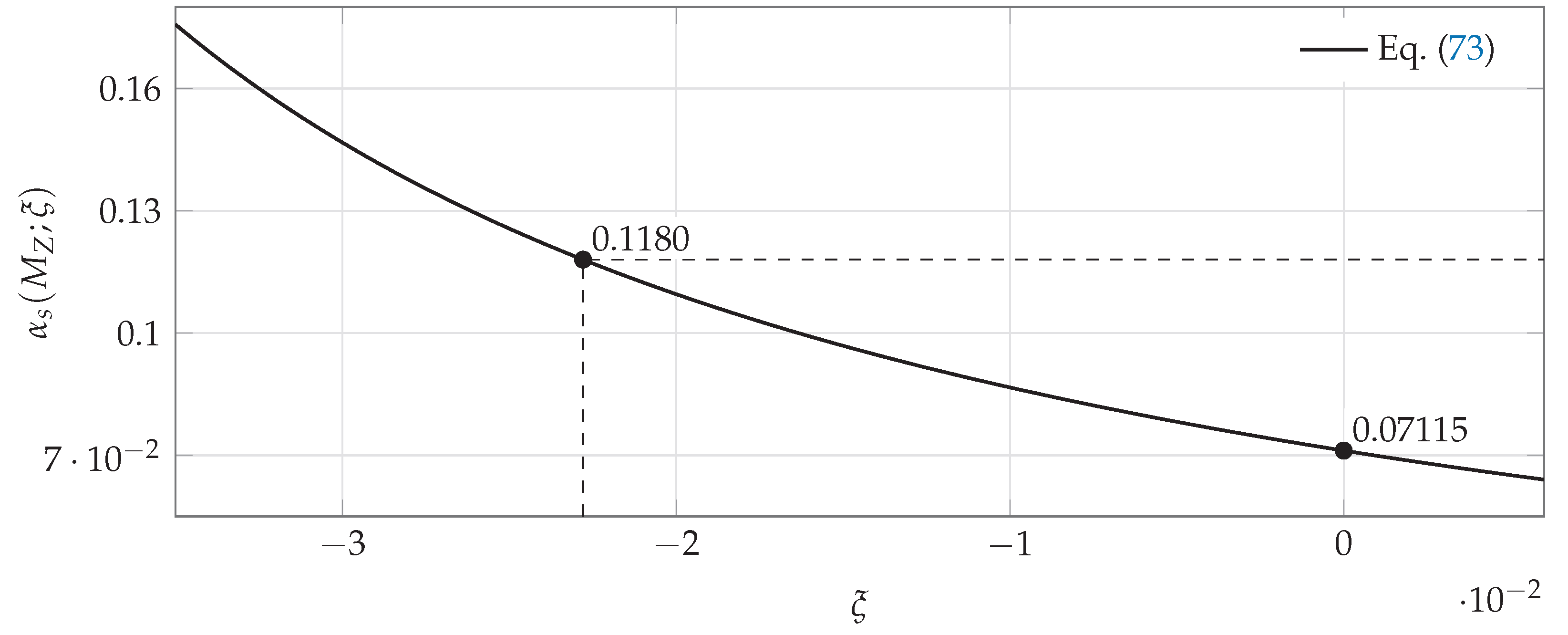

Table 1.
Normalized indices for one family of left-handed Weyl fermions. The final row has not yet been multiplied by the factor in Eq. (42).
Table 1.
Normalized indices for one family of left-handed Weyl fermions. The final row has not yet been multiplied by the factor in Eq. (42).
| Representation | |||
|---|---|---|---|
| 1 | |||
| 0 | |||
| 0 | |||
| 0 | |||
| 0 | 0 | ||
| Total | 2 | 2 | 2 |
Disclaimer/Publisher’s Note: The statements, opinions and data contained in all publications are solely those of the individual author(s) and contributor(s) and not of MDPI and/or the editor(s). MDPI and/or the editor(s) disclaim responsibility for any injury to people or property resulting from any ideas, methods, instructions or products referred to in the content. |
© 2026 by the authors. Licensee MDPI, Basel, Switzerland. This article is an open access article distributed under the terms and conditions of the Creative Commons Attribution (CC BY) license (http://creativecommons.org/licenses/by/4.0/).
Copyright: This open access article is published under a Creative Commons CC BY 4.0 license, which permit the free download, distribution, and reuse, provided that the author and preprint are cited in any reuse.