

Submitted:
08 September 2026
Posted:
09 September 2026
You are already at the latest version
Abstract
Reliable road-accident analysis requires attention to numerical stability, appropriate exposure treatment, and temporal validation in addition to predictive accuracy. This study presents an integrated numerical and machine-learning analysis of road accidents in Bangladesh using four synchronized datasets covering 2023–2025, with 288 divi-sion-month observations and a 36-month national series. The data include 17,046 acci-dents, 15,994 fatalities, and 20,389 injuries. The analysis combines singular-value and condition-number diagnostics, Normal Equation, QR, SVD and Tikhonov solvers, scaled polynomial approximation, spline and Savitzky–Golay methods, Poisson and NB2 like-lihood models, Kalman/RTS state-space estimation, Fourier analysis, and fifteen statistical and machine-learning models evaluated by leave-one-year-out validation. The fatali-ty-design matrix was full rank with κ(X)=16.73, while scaling reduced the cubic Van-dermonde condition number from 6.21×10⁴ to 7.77. Poisson was preferred to NB2 for conditional fatality analysis, and Fourier analysis identified a dominant 12-month cycle. Ridge regression, Huber regression, and Poisson random forest gave the best predictive results for accidents, fatalities, and injuries, respectively. Barishal recorded the highest annualized fatality rate at 5.44 per 100,000 population. These results show that combining numerical analysis with time-aware predictive modelling improves the robustness and interpretability of road-safety assessment in Bangladesh.
Keywords:
road accidents
; numerical analysis
; machine learning
; numerical stability
; Poisson regression
; Kalman filtering
; Fourier analysis
1. Introduction
Road-traffic crashes are difficult to model because they do not arise from a single cause. Exposure, road geometry, vehicle mix, driver behavior, enforcement, emergency response, reporting quality, and seasonal variation all influence the number and severity of crashes observed in a given place and time. This complexity has pushed road-safety research well beyond simple descriptive counts. Current work includes multidimensional severity prediction [1], IoT- and vision-based emergency-response systems [2], simulation-assisted accident reconstruction [3], motorcycle-specific risk analysis [4], multi-road-user safety simulation [5], rural–urban temporal scaling [6], large-language-model-assisted investigation of crash causation [7], and GIS-based hotspot detection in Bangladesh [8].
Machine learning has widened the range of tools available for such problems, particularly where nonlinear relationships and interactions are difficult to specify in advance. Reviews of artificial intelligence in crash-severity prediction show a rapid increase in the use of ensemble learning, deep learning, and hybrid approaches [9,11]. Seasonal and demographic analyses nevertheless continue to show that time structure matters [10], while rule-based generative-AI systems are beginning to appear in traffic-accident detection and interpretation [12]. More focused studies have used machine learning for accident prediction [32], compared statistical and machine-learning approaches for severity classification [33], developed AI-based pedestrian crash models [34], applied machine learning to crash and hotspot prediction [35], and proposed improved learning algorithms for severity estimation [36]. These studies confirm the value of flexible predictive models, but they also highlight a familiar problem: high predictive complexity does not by itself ensure that a model is numerically stable, interpretable, or reliable outside the sample on which it was trained.
For that reason, mathematical and statistical modelling remains central to road-safety research. Mathematical formulations have been used to study accident mechanisms and safety interventions [13], while data-driven models have been applied to broader crash-prediction tasks [14]. Time-series methods such as SARIMA and Prophet have been used to represent temporal dependence and changepoints [15], and ensemble methods have been explored for crash-severity prediction [16]. In Bangladesh, mathematical modelling has been used to examine factors associated with the growth of road accidents [17], and Poisson regression has been applied to crash-frequency modelling [18]. Other studies have considered operational traffic optimization under accident conditions [19], SEIR-type representations of accident severity [20], severity classification [21], alternative crash-prediction formulations [22], mathematical approaches to road-safety management [23], and data-based estimation of vehicle-crash parameters and dynamic crash response [24,25]. This body of work shows that road-safety analysis is not a single modelling problem; it may involve approximation, likelihood estimation, numerical linear algebra, dynamic state estimation, and supervised prediction.
The reliability of any of these methods also depends on the data on which they are built. Modern road-safety databases may combine administrative records, geospatial information, sensor data, connected-vehicle data, and other digital sources, each with its own limitations [26]. Descriptive studies have shown the importance of contextual and catastrophic crash factors [27], while conventional accident analyses remain useful for identifying broad burden patterns [28]. Risk-indicator studies further demonstrate that geographic priorities can change when different exposure denominators are used [29]. Data-mining research also shows that preprocessing, harmonization, missing-value treatment, and feature construction can materially affect the final results [30]. For Bangladesh, the authors' earlier work combined nonlinear deterministic, exposure-adjusted count, and seasonal time-series models [31]. That study provided a useful foundation, but it also pointed to the need for a framework that gives greater attention to numerical stability and out-of-time predictive performance.
Several gaps therefore remain. Numerical conditioning is seldom reported in road-safety studies, even though coefficient estimates may become unstable when predictors are poorly scaled or nearly dependent. Matrix rank, singular values, condition numbers, and perturbation sensitivity are often omitted from otherwise detailed modelling studies. Regularization is also commonly treated only as a prediction tool, rather than as a way of stabilizing a numerical system. In count modelling, Poisson and negative-binomial formulations are frequently chosen without fully examining whether the assumed mean–variance relationship matches the data under the selected exposure definition. Temporal studies, meanwhile, often rely on a single forecasting or smoothing technique rather than comparing interpolation, numerical differentiation, latent-state filtering, and spectral structure. A further concern is validation: many predictive studies still use random train–test splits, although neighbouring months and years are not independent and such splits can overstate generalization performance. These issues are especially relevant in Bangladesh, where mathematical, statistical, spatial, and machine-learning studies have generally developed along separate lines [8,17,20,31].
The present study addresses these gaps by combining numerical analysis and advanced machine learning within one reproducible framework. Numerical stability is examined using matrix rank, singular-value decomposition, condition numbers, normal equations, QR factorization, SVD pseudoinverse, Tikhonov regularization, generalized cross-validation, and controlled perturbation analysis. Polynomial trend estimation is accompanied by explicit examination of Vandermonde conditioning and time rescaling. Monthly fatality dynamics are studied using natural cubic splines, finite differences, Savitzky–Golay smoothing, Kalman filtering with Rauch–Tung–Striebel smoothing, and Fourier decomposition. Conditional fatality counts are modelled using Poisson and NB2 likelihoods with accident frequency incorporated as an exposure offset. Alongside these numerical and statistical methods, fifteen predictive models are evaluated, including linear and regularized regression, robust regression, count generalized linear models, kernel and neighbour methods, tree ensembles, boosting algorithms, and two Adam-trained artificial neural networks.
The aim of the study is to develop a numerically reliable and temporally credible framework for analysing road-accident burden in Bangladesh from 2023 to 2025. The analysis examines how accidents, fatalities, and injuries vary across years and divisions after population standardization; whether the numerical systems used for inference and approximation are well conditioned; what count, smoothing, state-space, and spectral methods reveal about fatality dynamics; and how numerical and machine-learning models perform when an entire year is withheld from training. The emphasis is therefore not only on which model fits best, but on which conclusions remain credible after numerical diagnostics, exposure adjustment, and out-of-time validation are taken into account.
2. Materials and Methods
2.1. Study Design, Data Sources, and Analytical Units
This retrospective analytical study covers January 2023 through December 2025. The primary analytical unit is the division-month, comprising eight administrative divisions observed over 36 consecutive months and yielding a balanced panel of 288 observations. Aggregation across divisions produces a 36-point national monthly series used for interpolation, numerical differentiation, state-space filtering, and spectral analysis. Four synchronized datasets are employed: 2022 division-level population statistics, the principal monthly road-accident panel, fatalities by vehicle type and division, and recorded vehicle counts by vehicle type and division. The overall analytical workflow, from data sources and preprocessing through numerical/statistical modelling, advanced machine learning, time-aware validation, model comparison, and road-safety interpretation, is summarized in Figure 1. The processed-data provenance is documented in the authors’ earlier Bangladesh road-safety study, which identifies Bangladesh Road Transport Authority road-accident statistics and Bangladesh Bureau of Statistics population statistics as the underlying public sources [31].
The complete analytical workflow was implemented in Python using NumPy, pandas, SciPy, Matplotlib, scikit-learn, and openpyxl. A fixed random seed of 42 was used for stochastic procedures, and bootstrap uncertainty was estimated using 5,000 resamples. The script also exports cleaned tables, a consolidated Excel workbook, solver diagnostics, cross-validated predictions, model metrics, a cleaning log, and reproducibility metadata to support transparent and reproducible analysis.
As summarized in Table 1, the main panel is complete for the variables used in modelling, whereas the vehicle files contain sparse missingness. Known division and vehicle-label inconsistencies are harmonized to canonical labels while retaining source values in the audit workflow. Numeric fields are validated, invalid values are converted to missing, analytical keys are checked for duplicates, and a first-of-month date index is constructed. Temporal ordering is preserved throughout.
2.2. Outcomes, Exposure Definitions, and Leakage Control
Let A_it, F_it, and I_it denote accidents, fatalities, and injuries for division i in month t, and let P_i denote the corresponding 2022 population. For a Y-year observation window, the annualized fatality rate per 100,000 persons is defined by
Rᶠᵢ = (100000 / Y) [ (Σₜ Fᵢₜ) / Pᵢ ]. (1)
The population denominator is intentionally fixed at 2022 values. Thus, the rate is a standardized three-year comparison rather than an estimate that incorporates annual population change. Division uncertainty is quantified from 5,000 nonparametric bootstrap resamples of monthly rates and percentile 95% confidence intervals.
Predictive leakage is controlled by excluding variables algebraically derived from each target. Fatalities-per-accident is therefore excluded when fatalities are predicted, and injuries-per-accident is excluded for injuries. Observed accident count is retained as an exposure-like covariate for conditional fatality and injury modelling; consequently, those predictions are interpreted as consequence models conditional on accident frequency, not as pre-crash forecasts.
Continuous predictors entering scale-sensitive models are standardized as
zⱼ = (xⱼ - x̄ⱼ) / sⱼ, (2)
and categorical predictors are one-hot encoded within each training fold so that preprocessing parameters are learned without using the held-out year.
2.3. Numerical Linear Algebra and Solver Audit
For an n x p design matrix X, singular-value decomposition (SVD) is written as
X = U Σ Vᵀ, (3)
where U and V have orthonormal columns and Σ contains non-negative singular values. Numerical sensitivity is summarized by the 2-norm condition number
κ₂(X) = σmax(X) / σmin(X). (4)
Four coefficient solvers are compared under the same linear model. The normal-equation estimator is
β̂_NE = (XᵀX)⁻¹ Xᵀy, (5)
whereas a thin QR factorization X = QR gives
β̂_QR = R⁻¹ Qᵀy. (6)
The SVD pseudoinverse solution is
β̂_SVD = V Σ⁺ Uᵀ y, (7)
where Σ+ reciprocates nonzero singular values subject to numerical tolerance. Tikhonov regularization uses
β̂_λ = (XᵀX + λD)⁻¹ Xᵀy, (8)
with D equal to the identity except for a zero intercept entry. Generalized cross-validation (GCV) selects λ using the smoothing matrix H_λ = X(XᵀX+λD)⁻¹Xᵀ:
GCV(λ) = n ||(I - H_λ)y||₂² / [n - tr(H_λ)]². (9)
The solver audit evaluates residual error, condition number, and sensitivity to controlled perturbations. This distinction is important because normal equations square the singular-value ratio, so κ₂(XᵀX) is approximately κ₂(X)² for a full-rank system.
2.4. Polynomial Approximation, Spline Interpolation, and Numerical Differentiation
To avoid the severe scaling of raw powers of month index t, time is mapped to [-1,1]:
xₜ = 2(t - tmin)/(tmax - tmin) - 1. (10)
For degree d, the Vandermonde matrix V_d = [1, x, x², ..., xᵈ] is fitted by least squares:
β̂(d) = arg min_β ||V_d β - y||₂². (11)
Degrees 1-8 are evaluated by leave-one-out cross-validation (LOOCV) on the 36-month national fatality series. Both raw- and scaled-basis condition numbers are reported to separate approximation error from numerical instability.
A natural cubic spline S(t) with zero second derivative at the two boundaries interpolates the national fatality series. Because exact interpolation can amplify local noise in derivatives, the analytical spline derivative is compared with second-order finite differences,
y'(t) ≈ [y(t+h) - y(t-h)] / (2h), h = 1 month, (12)
and with Savitzky-Golay local-polynomial smoothing. For a symmetric window j = -m,...,m and polynomial degree p, the local coefficients solve
minₐ Σⱼ₌₋ₘᵐ [ yₜ₊ⱼ - Σᵣ₌₀ᵖ aᵣ jʳ ]², ŷₜ = a₀. (13)
Agreement in derivative sign across methods is treated as stronger evidence of a turning direction than agreement in peak amplitude.
2.5. Exposure-Adjusted Poisson and Negative-Binomial Likelihoods
Fatality counts are modelled conditionally on accident frequency using log(A_it) as an offset. The Poisson specification is
Fᵢₜ ~ Poisson(μᵢₜ), log μᵢₜ = log Aᵢₜ + xᵢₜᵀβ. (14)
The covariate vector contains standardized year index, sine and cosine month terms, population, population density, dependency ratio, literacy rate, and seasonal indicators. Division fixed effects are omitted from this inferential specification because the division-level demographic predictors are time-invariant and would become exactly collinear with a complete division indicator set.
For the NB2 alternative, the conditional mean remains μ while variance is
Var(Fᵢₜ | xᵢₜ) = μᵢₜ + α μᵢₜ², α ≥ 0. (15)
Using r = 1/α, the NB2 probability mass function is
P(F=f) = Γ(f+r)/[Γ(r)Γ(f+1)] [r/(r+μ)]ʳ [μ/(r+μ)]ᶠ. (16)
Poisson and NB2 parameters are estimated by direct numerical maximum likelihood. Model support is compared using log-likelihood, AIC, BIC, and Poisson Pearson dispersion. For a standardized predictor coefficient β_j, the incidence-rate ratio is
IRRⱼ = exp(βⱼ). (17)
2.6. Local-Linear-Trend Kalman Filter and RTS Smoother
The national fatality series is also represented as a noisy observation of a latent local level and slope. With state vector s_t = [ℓ_t, b_t]^T, the transition equation is
sₜ = G sₜ₋₁ + wₜ, G = [[1,1],[0,1]], wₜ ~ N(0,Q), (18)
and the observation equation is
yₜ = H sₜ + vₜ, H = [1,0], vₜ ~ N(0,R). (19)
The Kalman prediction and correction equations are
sₜ⁻ = Gsₜ₋₁; Pₜ⁻ = GPₜ₋₁Gᵀ+Q; Kₜ = Pₜ⁻Hᵀ(HPₜ⁻Hᵀ+R)⁻¹; sₜ = sₜ⁻ + Kₜ(yₜ-Hsₜ⁻). (20)
Variance parameters are estimated by maximizing the Gaussian innovation likelihood. The Rauch-Tung-Striebel (RTS) backward recursion smooths filtered states using
Jₜ = PₜGᵀ(Pₜ₊₁⁻)⁻¹, sₜ|T = sₜ + Jₜ(sₜ₊₁|T - sₜ₊₁⁻). (21)
2.7. Fourier Decomposition
A linear trend is removed before fast Fourier transformation. If z_t denotes the detrended series, a K-harmonic reconstruction is
ŷₜ = a + bt + Σₖ₌₁ᴷ Aₖ cos(2π fₖ t + φₖ). (22)
Spectral components are ranked by power, periods are reported as 1/f_k months, and the four strongest non-zero harmonics are retained for reconstruction. With only 36 monthly observations, periodicity is interpreted as evidence of recurring structure rather than as a precise long-horizon frequency estimate [6,15].
2.8. Time-Aware Statistical and Machine-Learning Models
Fifteen predictive model families are compared under identical preprocessing: ordinary least squares, Ridge, Elastic Net, Huber robust regression, Poisson GLM, Tweedie compound-Poisson GLM, RBF support-vector regression, distance-weighted KNN, two- and three-hidden-layer neural networks trained with Adam, random forest, Poisson random forest, Extra Trees, Huber gradient boosting, and Poisson histogram gradient boosting. The expanded library spans linear, regularized, robust, count-aware, kernel, local-neighbor, neural, bagging, and boosting structures. Key computational settings from the reproducible analysis script are listed in Table 2.
For ordinary linear regression, the empirical squared-error objective is
β̂_OLS = arg min_β Σᵢ (yᵢ - xᵢᵀβ)². (23)
Ridge regression solves
β̂_R = arg min_β { Σᵢ (yᵢ - xᵢᵀβ)² + α||β||₂² }, (24)
while Elastic Net solves
β̂_EN = arg min_β { (1/2n)||y-Xβ||₂² + α[ρ||β||₁ + (1-ρ)||β||₂²/2] }. (25)
Huber regression minimizes a robust loss plus L2 regularization, with residual loss
Lδ(r) = 0.5r² if |r|≤δ; δ(|r|-0.5δ) otherwise. (26)
The Poisson GLM uses a logarithmic mean link
μᵢ = exp(xᵢᵀβ), (27)
whereas the Tweedie compound-Poisson model uses the variance function
Var(Yᵢ|xᵢ) = φ μᵢᵖ, p = 1.5. (28)
RBF support-vector regression uses the kernel K(x,x') = exp[-γ||x-x'||²] and the ε-insensitive primal objective
min 0.5||w||² + CΣᵢ(ξᵢ+ξᵢ*), subject to |yᵢ-f(xᵢ)| ≤ ε + slack. (29)
Distance-weighted KNN predicts from the k nearest training observations as
ŷ(x) = [Σⱼ∈Nₖ(x) d(x,xⱼ)⁻¹ yⱼ] / [Σⱼ∈Nₖ(x) d(x,xⱼ)⁻¹]. (30)
For the neural networks, hidden-layer propagation is
h⁽ˡ⁾ = ReLU(W⁽ˡ⁾h⁽ˡ⁻¹⁾ + b⁽ˡ⁾), ŷ = W⁽ᴸ⁾h⁽ᴸ⁻¹⁾ + b⁽ᴸ⁾. (31)
Adam updates first and second gradient moments and then the parameters:
mₜ=β₁mₜ₋₁+(1-β₁)gₜ; vₜ=β₂vₜ₋₁+(1-β₂)gₜ²; θₜ=θₜ₋₁-η m̂ₜ/(√v̂ₜ+ε). (32)
Bagged tree ensembles predict by averaging B regression trees,
ŷ_RF(x) = (1/B) Σᵦ₌₁ᴮ Tᵦ(x), (33)
with Poisson random forest changing the node-split criterion and Extra Trees increasing split randomization. Gradient boosting constructs an additive predictor
f_M(x) = f₀(x) + Σₘ₌₁ᴹ ν hₘ(x), (34)
where each h_m approximates the negative gradient of the selected loss; Huber and Poisson losses are used for the two boosting variants.
2.9. Temporal Validation and Performance Metrics
Validation uses GroupKFold with calendar year as the grouping variable, generating three leave-one-year-out folds: train on two years and predict the omitted year. No headline result is based on a random split. For observations y_i and out-of-fold predictions ŷ_i, root-mean-square error is
RMSE = √[(1/n) Σᵢ (yᵢ-ŷᵢ)²], (35)
mean absolute error is
MAE = (1/n) Σᵢ |yᵢ-ŷᵢ|, (36)
and the coefficient of determination is
R² = 1 - [Σᵢ(yᵢ-ŷᵢ)² / Σᵢ(yᵢ-ȳ)²]. (37)
Symmetric mean absolute percentage error is
SMAPE = (100/n) Σᵢ [2|yᵢ-ŷᵢ|/(|yᵢ|+|ŷᵢ|)], (38)
and normalized RMSE is
NRMSE(%) = 100 × RMSE / ȳ. (39)
For positive count predictions, mean Poisson deviance is
D_P = (2/n) Σᵢ [ yᵢ log(yᵢ/ŷᵢ) - (yᵢ-ŷᵢ) ], (40)
with the convention y log(y/ŷ)=0 at y=0. Spearman rank correlation is also reported. Model selection within each target is based on minimum out-of-fold RMSE, with NRMSE used for cross-outcome comparisons.
2.10. Vehicle-Exposure Screening Ratio
Vehicle fatality and recorded-vehicle files are matched by year, month, division, and harmonized vehicle type. Only non-missing records with strictly positive recorded-vehicle denominators are eligible. For vehicle type v,
VFRᵥ = 100 × [Σ Fᵥ / Σ Vᵥ]. (41)
The quantity is explicitly described as fatalities per 100 recorded vehicles. Because the denominator is a source-defined recorded count rather than verified registered-fleet exposure or vehicle-kilometres travelled, VFR is a descriptive screening indicator and not a causal or actuarial fatality probability.
3. Results
3.1. National Burden and Annual Change
Across 2023-2025, the synchronized panel contains 17,046 accidents, 15,994 fatalities, and 20,389 injuries. Table 3 shows that the three outcomes do not move in parallel. Accidents increased by 6.57% in 2024 and then decreased by 2.75% in 2025; fatalities increased by 9.08% in 2024 and remained almost unchanged in 2025 (+0.18%); injuries fell by 13.68% in 2024 and by another 0.71% in 2025.
Figure 2 visualizes the divergence. The 2024 increase in accident frequency and fatal burden occurred simultaneously with a marked injury reduction, while the 2025 reduction in accidents did not produce a reduction in fatalities. This supports modelling accidents, fatalities, and injuries as related but non-interchangeable outcomes [16,21,22].
3.2. Spatial Disparity and Bootstrap Uncertainty
Population standardization materially changes geographic prioritization. Table 4 ranks the eight divisions using fixed 2022 population exposure. Barishal has the highest annualized fatality rate (5.44 per 100,000), followed by Sylhet (4.44) and Rajshahi (3.83), whereas Rangpur (2.23) and Khulna (2.29) are lowest.
Figure 3 presents the ranked annualized rates and confirms that high raw-count divisions are not necessarily the highest-rate divisions. The figure therefore emphasizes the distinction between scale and standardized burden.
3.3. Correlation, Rank, and Numerical Conditioning
Figure 5 shows strong dependence among several safety and demographic variables. Accidents and fatalities are highly correlated (r=0.969), accidents and injuries are positively correlated (r=0.762), population correlates with accidents (r=0.735) and fatalities (r=0.743), and population density correlates with fatalities (r=0.595). These relationships motivate multivariable modelling while also making numerical diagnostics necessary.
Table 5 summarizes the core conditioning diagnostics. The inferential fatality design is full rank (11/11), with κ2(X)=16.73 and κ2(XᵀX)=279.97. The largest and smallest singular values are 26.517 and 1.585. In contrast, the raw cubic Vandermonde matrix is severely ill-conditioned until the time coordinate is scaled.
Figure 5 displays the singular-value spectrum. Its gradual decline, rather than collapse toward a nearly zero terminal singular value, supports the full-rank diagnosis and indicates that the inferential coefficient system is not dominated by one near-null direction.
Figure 6 evaluates ridge stabilization. The normal-equation system begins near a condition number of 279.97 and reaches a minimum near 4.79 around λ≈355.4 before rising at very large λ because the intercept is deliberately unpenalized. The non-monotonic path demonstrates why regularization should be inspected numerically rather than assumed to improve conditioning without limit.
Figure 7 isolates polynomial-basis conditioning. At the LOOCV-selected degree 3, scaling the month coordinate from its raw integer form to [-1,1] reduces κ(V) from 6.21×10^4 to 7.77. At degree 8, the raw condition number reaches approximately 6.21×10^12, whereas the scaled basis remains several orders of magnitude better conditioned.
3.4. Polynomial Trend, Smoothing, and Numerical Derivatives
LOOCV selects a cubic polynomial for the national fatality series. The degree-3 fit RMSE is 78.13 and LOOCV RMSE is 84.80. Increasing degree beyond three provides only modest in-sample improvement while worsening out-of-sample error and rapidly inflating the raw-basis condition number. Selected numerical time-series diagnostics are summarized in Table 6.
Figure 8 compares observed fatalities with the exact natural cubic spline, the LOOCV-selected cubic polynomial, and the Savitzky-Golay smoothed trend. The spline passes through every observation, the cubic polynomial captures broad low-frequency movement, and Savitzky-Golay smoothing preserves major turning behaviour while attenuating local noise.
Figure 9 compares first derivatives from the exact spline, second-order finite differences, and Savitzky-Golay smoothing. Around the pronounced mid-2024 decline, the approximate minima are -323, -206, and -88 fatalities per month, respectively. All methods agree on direction and timing, but the exact interpolant produces the largest amplitude; consequently, derivative sign is more robust than peak magnitude.
3.5. Time-Aware Predictive Performance
Predictive ranking is strongly outcome-specific under leave-one-year-out validation. Figure 10 compares NRMSE across the complete statistical and machine-learning library. Regularized and robust linear models remain competitive for accidents and fatalities, whereas a count-aware random forest is preferred for injuries. Neural networks converge successfully but do not dominate out-of-time performance.
Table 7 reports the best machine-learning/statistical model for each outcome. Ridge regression is best for accidents (RMSE=24.20; R²=0.467), Huber robust regression is best for fatalities (RMSE=7.97; R²=0.937), and Poisson random forest is best for injuries (RMSE=29.89; R²=0.633). The fatality result should be interpreted conditionally on observed accident frequency.
Figure 11, Figure 12 and Figure 13 provide observed-versus-predicted diagnostics for the three best target-specific models. Figure 11 shows that accident predictions follow the one-to-one trend but shrink toward the centre, consistent with the moderate R².
Figure 12 shows a substantially tighter relationship for fatalities under Huber robust regression, consistent with R²=0.937 and Spearman ρ=0.971.
Figure 13 shows the injury predictions from Poisson random forest. The model captures the principal ordering and much of the outcome spread, although extreme observations retain larger residuals.
3.6. Vehicle-Exposure Screening Patterns
Among matched observations with positive recorded-vehicle denominators, motorcycles have the highest overall exposure-style fatality ratio at 85.24 fatalities per 100 recorded vehicles, followed by auto rickshaws (81.68), other vehicles (70.01), easy bikes (66.06), and vans (61.47). Table 8 lists the eight highest categories.
Figure 14 visualizes the overall vehicle ranking. The concentration of high values among motorcycles and paratransit categories is consistent with literature emphasizing motorcycle and vulnerable-road-user risk [4,27], but the source-defined denominator requires cautious interpretation.
Figure 15 demonstrates substantial division-by-vehicle heterogeneity. Some cells exceed 100 fatalities per 100 recorded vehicles; this does not represent a probability greater than one because the denominator is an aggregated source-defined recorded count rather than a fixed cohort at risk. The heat map therefore strengthens the denominator-sensitivity warning.
3.7. Poisson Versus NB2 Conditional Fatality Inference
Both direct maximum-likelihood optimizations converge. Table 9 shows that Poisson attains log-likelihood -953.50, AIC 1928.99, and BIC 1969.28, whereas NB2 produces log-likelihood -953.55, AIC 1931.09, and BIC 1975.05. The NB2 overdispersion parameter is only 7.33×10^-5 and Poisson Pearson dispersion is 0.969, indicating near-equidispersion under the accident-offset formulation.
Table 10 reports the principal Poisson incidence-rate ratios. A one-standard-deviation increase in year index is associated with a 1.9% increase in conditional fatality incidence (IRR=1.019, 95% CI 1.003-1.035, p=0.019), while a one-standard-deviation increase in population density is associated with a 5.2% increase (IRR=1.052, 95% CI 1.022-1.083, p<0.001). Other listed covariates are not significant at the 5% level.
Figure 16 shows observed and fitted fatalities for Poisson and NB2. The fitted curves are visually almost indistinguishable, exactly as expected when the estimated NB2 dispersion collapses toward zero. This supports diagnosing overdispersion for the specific outcome and exposure definition rather than transferring it mechanically from other crash-count formulations [18,22,31].
3.8. State-Space and Spectral Fatality Dynamics
Figure 17 presents the local-linear-trend Kalman/RTS estimate. The latent level is substantially smoother than the observed monthly series, while the state uncertainty band expands in portions of the series with larger observational departures. The state-space view treats month-to-month variation as a combination of latent evolution and measurement/process noise rather than interpreting every observed fluctuation as a structural shift.
Figure 18 shows the detrended Fourier power spectrum. The strongest non-zero component has a 12-month period (power 23,947; amplitude 51.58), followed by 9- and 6-month components. The annual component is therefore the clearest recurring frequency in the 36-month sample.
Figure 19 reconstructs the national series from the linear trend and four strongest harmonics. The reconstructed series has RMSE 52.46 and MAE 41.49, and the estimated linear component increases by approximately 1.14 fatalities per month over the study window. The reconstruction captures broad periodic structure without claiming precise long-horizon seasonality from only three annual cycles.
3.9. GCV-Selected Tikhonov Regularization and ANN Optimization
Figure 20 displays the GCV criterion together with the associated conditioning path for Tikhonov regularization. The selected regularization represents a compromise between fit and coefficient-system stability, and it becomes the strongest numerical baseline in the direct numerical-versus-ML comparison reported below.
Figure 21 shows the training-loss histories for the three-hidden-layer Adam networks across targets. The curves demonstrate successful optimization and early-stopping behaviour, but optimization convergence should not be confused with out-of-time predictive superiority.
3.10. Direct Comparison of Numerical Solvers and Machine Learning
The direct family comparison in Figure 25 uses NRMSE so that the three outcomes can be compared on the same relative scale. Tikhonov GCV is the best numerical solver for all three outcomes, whereas Ridge regression, Huber robust regression, and Poisson random forest are the best machine-learning/statistical models for accidents, fatalities, and injuries. Table 11 quantifies the margins.
Figure 26 compares annual out-of-time predictions from the best numerical and best machine-learning/statistical model. The plot makes clear that model-family differences are not constant across years; some years are captured similarly by both families, while others account for most of the relative-performance gap.
Figure 27 places all numerical and machine-learning models in a single NRMSE heat map. Table 12 reproduces the displayed values for auditability. The result is not a simple numerical-versus-ML dichotomy: Tikhonov GCV is nearly tied with Ridge for accidents and with Huber/Elastic Net for fatalities, while the larger advantage of Poisson random forest appears for injuries. ANN-3H-Adam produces NRMSE values of 79.0%, 23.9%, and 43.3% for accidents, fatalities, and injuries, respectively; successful neural optimization therefore does not guarantee superior temporal generalization.
4. Discussion
4.1. Principal Findings and Numerical Interpretation
This study produces four principal findings.
First, road-safety burden is outcome-specific and spatially heterogeneous: accidents, fatalities, and injuries follow different annual trajectories, and population standardization places Barishal and Sylhet above the larger divisions in annualized fatality burden.
Second, the main inferential design is numerically usable but not immune to sensitivity: κ2(X)=16.73 is moderate, whereas κ2(XᵀX)=279.97 illustrates the amplification created by normal equations. The polynomial subsystem provides the sharper warning because scaling reduces the cubic Vandermonde condition number by almost four orders of magnitude.
Third, the conditional fatality counts are close to equidispersed, so Poisson is more parsimonious than NB2 under the accident-offset specification.
Fourth, out-of-time performance is model- and outcome-specific: no single family dominates all targets.
The polynomial result is particularly relevant to applied mathematics. Increasing model degree can reduce in-sample residuals while simultaneously degrading both conditioning and cross-validated reconstruction. This is a concrete example of why approximation quality must be considered jointly with numerical sensitivity. The SVD spectrum, Ridge path, Tikhonov GCV curve, and raw-versus-scaled Vandermonde comparison together show that numerical diagnostics are not ancillary plots; they determine whether estimated coefficients and trends are reproducible under finite precision and small data perturbations [19,23,24,25].
4.2. Count Inference, Exposure, and Denominator Sensitivity
The Poisson-versus-NB2 comparison also illustrates why distributional assumptions should be evaluated against the exact modelling question. Count data are often assumed to require negative-binomial overdispersion, but here fatalities are modelled conditional on observed accident exposure. With Pearson dispersion 0.969 and NB2 alpha close to zero, the extra NB2 parameter is not supported by AIC or BIC. The significant positive association of population density with conditional fatality incidence is consistent with the idea that urban exposure and consequence mechanisms deserve attention, but the model remains associational rather than causal [18,22].
The vehicle-exposure analysis requires even greater care. Motorcycle and paratransit categories rank highly, consistent in direction with motorcycle-risk and catastrophic-factor studies [4,27], yet the denominator is a source-defined recorded-vehicle count. A ratio above 100 in some division-vehicle cells is mathematically possible under this aggregate denominator and should not be interpreted as a probability. This is exactly the type of denominator problem highlighted by general risk-indicator and data-source research [26,29].
4.3. Temporal Dynamics and Model Generalization
The agreement between Fourier analysis and the smoothed time-series representations provides complementary evidence of recurring annual structure. The 12-month component is the strongest non-zero spectral frequency, while the Kalman/RTS model separates a slowly evolving latent level from short-term observation noise. These approaches answer different questions: Fourier analysis characterizes recurrent periodic components, whereas state-space estimation asks how the latent level evolves when observations are noisy. The result aligns with prior seasonal forecasting and scaling studies [6,10,15].
The predictive results reinforce the importance of temporal validation. Ridge regression for accidents, Huber regression for fatalities, and Poisson random forest for injuries outperform more complex alternatives on their respective targets. ANN-2H and ANN-3H models achieve stable training convergence, yet their NRMSE values do not establish superiority. This finding is consistent with broader reviews warning that high-capacity AI can underperform when samples are small, temporally structured, or weakly informative [9,11]. The practical implication is that model sophistication should be justified by out-of-time evidence rather than by architecture alone.
The direct numerical-versus-ML comparison adds an applied-mathematical perspective that is often missing from road-safety benchmarking. Tikhonov GCV remains within 0.2-0.3 NRMSE percentage points of the best data-driven model for fatalities and accidents, respectively, while the advantage of Poisson random forest becomes more visible for injuries. This pattern suggests that regularized numerical solvers can serve as strong transparent baselines. Machine learning should be interpreted as an incremental modelling choice whose value depends on outcome structure, not as a universal replacement for numerical methods.
4.4. Policy Relevance
For road-safety management in Bangladesh, three implications follow. First, geographic prioritization should report both absolute burden and population-standardized rates because these lead to different rankings. Second, conditional fatality models can identify covariate associations and consequence patterns after accounting for accident exposure, but they should not be described as crash-occurrence models. Third, operational model selection should use future-period or leave-period-out validation whenever deployment will occur in a later year. GIS hotspot analysis in Bangladesh [8], data-mining frameworks [30], and the authors' prior national modelling [31] provide complementary tools that could be integrated with the present numerical diagnostics in future decision-support systems.
4.5. Limitations and Future Work
The study has several limitations. The panel is aggregated at division-month level and spans only three years, limiting the identification of rare events, local roadway mechanisms, and long-period spectral components. Population is fixed at 2022 values, so rates are standardized comparisons rather than dynamic demographic rates. Vehicle-count denominators are source-defined and are not equivalent to registered fleet, traffic volume, or vehicle-kilometres travelled. Accident count is used as an exposure-like predictor for fatality and injury models, which improves conditional consequence prediction but prevents interpretation as a pre-crash forecast. Finally, no model can correct under-reporting, source-definition changes, or omitted roadway/weather/driver variables that are absent from the administrative data.
Future research should extend the panel temporally, incorporate crash-location geometry, roadway design, weather, enforcement, traffic volume, and emergency-response variables, and test geographic transfer across finer spatial units. Hierarchical Bayesian or spatiotemporal count models could explicitly represent spatial dependence; causal designs could address intervention effects; and external validation on a later, completely unseen year would provide a stronger deployment test. For machine learning, nested temporal tuning, calibrated uncertainty, explainability, and model-drift monitoring should accompany any move from retrospective benchmarking to operational prediction [7,9,11,12].
5. Conclusions
An integrated numerical and machine-learning analysis of Bangladesh road accidents during 2023-2025 shows that numerical reliability and temporal generalization are as important as predictive flexibility. The fatality design matrix is full rank with moderate conditioning, but raw polynomial time bases become severely ill-conditioned; scaling the cubic Vandermonde system reduces κ(V) from 6.21×10^4 to 7.77. Conditional fatality counts are nearly equidispersed, and Poisson is preferred to NB2 by AIC/BIC. The national fatality series contains a dominant 12-month component, while spline, finite-difference, Savitzky-Golay, and Kalman/RTS methods provide complementary views of local change and latent trend.
Under leave-one-year-out validation, Ridge regression is best for accidents, Huber robust regression for fatalities, and Poisson random forest for injuries. Tikhonov GCV remains a competitive transparent numerical baseline, especially for accidents and fatalities, whereas the ANN models demonstrate that successful optimization does not guarantee best out-of-time performance. Population-standardized burden is highest in Barishal at 5.44 fatalities per 100,000. Overall, the study supports a road-safety workflow in which exposure definitions, numerical conditioning, likelihood adequacy, and temporal validation are checked before policy conclusions are drawn.
Author Contributions
Sree Pradip Kumer Sarker contributed to conceptualization, methodology, software, validation, formal analysis, investigation, resources, data curation, writing original draft preparation, writing review and editing, and visualization. Md Shahid Mamun provided supervision throughout all stages of the research, including study design, methodology refinement, manuscript review and editing, and overall guidance. All authors have read and agreed to the published version of the manuscript.
Funding
This research received no external funding.
Data Availability Statement
The data supporting the findings of this study are included within the article in the form of tables and figures. The processed datasets used for analysis were compiled from publicly available official statistics published by the Bangladesh Road Transport Authority (BRTA) and BBS population statistics. No additional datasets were generated beyond those presented in this manuscript.
Acknowledgments
The authors gratefully acknowledge the Department of Civil Engineering, Ahsanullah University of Science and Technology (AUST), Dhaka, Bangladesh, for providing academic guidance, research support, and a conducive environment for conducting this study. The authors also acknowledge the BRTA and BBS for making the official road accident and population statistics publicly available, which formed the basis of this research.
Conflicts of Interest
The authors declare no conflicts of interest.
Abbreviations
| AIC | Akaike information criterion |
| ANN | Artificial neural network |
| BIC | Bayesian information criterion |
| FFT | Fast Fourier transform |
| GCV | Generalized cross-validation |
| GLM | Generalized linear model |
| KNN | k-nearest neighbors |
| LOOCV | Leave-one-out cross-validation |
| NB2 | Negative-binomial type 2 |
| NRMSE | Normalized root-mean-square error |
| RBF | Radial basis function |
| RMSE | Root-mean-square error |
| RTS | Rauch-Tung-Striebel |
| SVD | Singular-value decomposition |
| SVR | Support-vector regression |
References
- Chao, H. Using multidimensional analysis to predict the severity of traffic accidents and their contributing factors. ITM Web Conf. 2026, 84, 03002. [Google Scholar] [CrossRef]
- Noor, A.; Almukhalfi, H.; Noor, T.H.; Ranjan, R. TAERM: Traffic accident emergency response management framework for detection and classification using IoT and YOLOv9. Future Gener. Comput. Syst. 2026, 181, 108444. [Google Scholar] [CrossRef]
- Ignácz, F.; Moser, A.; Kőfalvi, G.; Feszty, D.; Lakatos, I. Simulation of the turning assistant in road traffic accident reconstruction. Future Transp. 2026, 6, 13. [Google Scholar] [CrossRef]
- Kozłowski, E.; Traczyński, M.; Skoczyński, P.; Jaskowski, P.; Madlenak, R. Risk factor analysis of single motorcycle accidents in road traffic. Appl. Sci. 2026, 16, 1629. [Google Scholar] [CrossRef]
- Fu, T.; Wang, J.; Wang, J.; Shangguan, Q.; Xie, S. Multi-road-user simulation platform for traffic safety analysis: Platform design and applications. Simul. Model. Pract. Theory 2026, 150, 103298. [Google Scholar] [CrossRef]
- Copsey, I.; Hanley, Q.; Sutton, J. Monthly rural-urban scaling of road accidents in England, Wales and Scotland (2019–2023). Appl. Math. Comput. 2026, 516, 129874. [Google Scholar] [CrossRef]
- Dai, B.; Wang, X.; Yang, F.; Feng, Y.; Wang, Y.; Quddus, M. Leveraging large language models for crash causation chain inference with in-depth accident investigation data. Transp. Res. Part C Emerg. Technol. 2026, 191, 105820. [Google Scholar] [CrossRef]
- Billah, M.; Shaik, M.E.; Hossain, M.S.; Sakib, S.E.J.; Rahman, L. Identification and analysis of road traffic crash hotspots using Geographic Information System (GIS): A study on Dhaka–Mawa Expressway (N804), Bangladesh. J. Sens. 2026, 2026, 5619948. [Google Scholar] [CrossRef]
- Alobidan, Y.A.; Soh, B.; Li, A.; Almudayni, Z. Artificial intelligence for predicting road accident severity: A global systematic review. Results Eng. 2026, 31, 111289. [Google Scholar] [CrossRef]
- Mahdi, A.J.; Ismael, K. Analyzing and predicting traffic accident trends considering gender and seasonal patterns: A case study of Al-Sulaymaniyah City. Eur. Transp. Trasp. Eur. 2026, 106, Paper 7. [Google Scholar]
- Affou, H.; Teso-Fz-Betoño, D.; Fernandez-Gamiz, U.; Ramos-Hernanz, J.A.; Caballero-Martin, D.; Lopez-Guede, J.M. Advances in traffic accident prediction: A survey of novel approaches. Urban Sci. 2026, 10, 349. [Google Scholar] [CrossRef]
- Raiyn, J. A generative AI-driven intelligent rules framework for traffic accident detection and analysis. Transp. Res. Interdiscip. Perspect. 2026, 36, 101916. [Google Scholar] [CrossRef]
- Bamel, K.; Jaglan, S.; Dass, S.; Bamel, K.; Khan, A.A.; Berwal, P.; Gupta, N. Mathematical modeling analysis of India's accident and use of fly ash and polymers in road safety. J. Polym. Compos. 2025, 13, S488–S499. [Google Scholar]
- Kiran, A.V.; Pavan, T.K.S.; Reddy, S.T.; Suchitra, S. Predictive modeling of traffic accidents: A data-driven approach. In Proceedings of the International Conference on Intelligent Systems and Digital Transformation (ICISD 2025); Dilip, G., et al., Eds.; Atlantis Highlights in Intelligent Systems , 2025; Volume 15. [Google Scholar]
- Agyemang, E.F.; Mensah, J.A.; Ocran, E.; Opoku, E.; Nortey, E.N.N. Time series based road traffic accidents forecasting via SARIMA and Facebook Prophet model with potential changepoints. Heliyon 2023, 9, e22544. [Google Scholar] [CrossRef] [PubMed]
- Alhadidi, T.; Elhenawey, M. Modeling crashes severity using ensemble techniques. Eurasia Proc. Sci. Technol. Eng. Math. 2023, 26, 357–365. [Google Scholar] [CrossRef]
- Biswas, A.; Tasnim, K.; Biswas, M.H.A. Mathematical modeling applied to assess the driving factors of increasing road accidents in Bangladesh. Khulna Univ. Stud. 2022, Special Issue ICSTEM4IR, 757–767. [Google Scholar] [CrossRef]
- Khan, M.K.; Hasan, M.T. A Poisson regression approach to modeling traffic accident frequency in urban areas. Am. J. Interdiscip. Stud. 2022, 3, 117–156. [Google Scholar] [CrossRef]
- Naumova, N.A. Application of mathematical modeling methods for operational optimization of urban traffic in an accident on a section of the road network. Civ. Eng. Archit. 2021, 9, 2140–2146. [Google Scholar] [CrossRef]
- Tasnim, K.; Biswas, A.; Biswas, M.H.A. Mathematical approach to assess the severity of road accidents in Bangladesh using a SEIR-type model. In Proceedings of the International Conference on Industrial & Mechanical Engineering and Operations Management, Dhaka, Bangladesh, 2020. [Google Scholar]
- Xi, J.; Guo, H.; Tian, J.; Liu, L.; Liu, H. A classification and recognition model for the severity of road traffic accident. Adv. Mech. Eng. 2019, 11, 1–8. [Google Scholar] [CrossRef]
- Abdulhafedh, A. Road crash prediction models: Different statistical modeling approaches. J. Transp. Technol. 2017, 7, 190–205. [Google Scholar]
- Ondrejka, R.; Moravčíková, L. Mathematical modelling within the road safety management. Acta Technol. 2015, 1, 5–8. [Google Scholar] [CrossRef]
- Pawlus, W.; Robbersmyr, K.G.; Karimi, H.R. Mathematical modeling and parameters estimation of a car crash using data-based regressive model approach. Appl. Math. Model. 2011, 35, 5091–5107. [Google Scholar] [CrossRef]
- Pawlus, W.; Nielsen, J.E.; Karimi, H.R.; Robbersmyr, K.G. Development of mathematical models for analysis of a vehicle crash. WSEAS Trans. Appl. Theor. Mech. 2010, 5. [Google Scholar]
- Gutierrez-Osorio, C.; Pedraza, C. Modern data sources and techniques for analysis and forecast of road accidents: A review. J. Traffic Transp. Eng. Engl. Ed. 2020, 7, 432–446. [Google Scholar] [CrossRef]
- Ashraf, I.; Hur, S.; Shafiq, M.; Park, Y. Catastrophic factors involved in road accidents: Underlying causes and descriptive analysis. PLoS ONE 2019, 14, e0223473. [Google Scholar] [CrossRef] [PubMed]
- Kumar, P.S.; Viswanadham, V.; Bharathi, B. Analysis of road accident. IOP Conf. Ser. Mater. Sci. Eng. 2019, 590, 012029. [Google Scholar] [CrossRef]
- Cioca, L.-I.; Ivascu, L. Risk indicators and road accident analysis for the period 2012–2016. Sustainability 2017, 9, 1530. [Google Scholar] [CrossRef]
- Kumar, S.; Toshniwal, D. A data mining framework to analyze road accident data. J. Big Data 2015, 2, 26. [Google Scholar] [CrossRef]
- Sarker, S.P.K.; Mamun, M.S. Mathematical modeling for road accident analysis in Bangladesh: Nonlinear deterministic, exposure-adjusted count, and seasonal time-series approaches. Int. J. Transp. Eng. Technol. 2026, 12, 98–118. [Google Scholar] [CrossRef]
- Ardakani, S.P.; Liang, X.; Mengistu, K.T.; So, R.S.; Wei, X.; He, B.; Cheshmehzangi, A. Road car accident prediction using a machine-learning-enabled data analysis. Sustainability 2023, 15, 5939. [Google Scholar] [CrossRef]
- Infante, P.; Jacinto, G.; Afonso, A.; Rego, L.; Nogueira, V.; Quaresma, P.; Saias, J.; Santos, D.; Nogueira, P.; Silva, M.; Costa, R.P.; Gois, P.; Manuel, P.R. Comparison of statistical and machine-learning models on road traffic accident severity classification. Computers 2022, 11, 80. [Google Scholar] [CrossRef]
- Meocci, M.; Branzi, V.; Martini, G.; Arrighi, R.; Petrizzo, I. A predictive pedestrian crash model based on artificial intelligence techniques. Appl. Sci. 2021, 11, 11364. [Google Scholar] [CrossRef]
- Santos, D.; Saias, J.; Quaresma, P.; Nogueira, V.B. Machine learning approaches to traffic accident analysis and hotspot prediction. Computers 2021, 10, 157. [Google Scholar] [CrossRef]
- Tang, J.; Huang, Y.; Liu, D.; Xiong, L.; Bu, R. Research on traffic accident severity level prediction model based on improved machine learning. Systems 2025, 13, 31. [Google Scholar] [CrossRef]
Figure 1.
Integrated methodological framework.
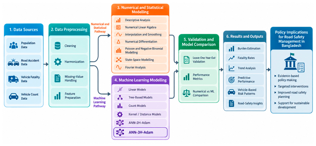
Figure 2.
Annual national accident, fatality, and injury totals, 2023-2025.
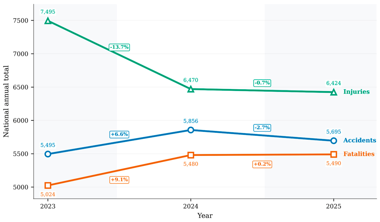
Figure 3.
Division-level annualized road-fatality rates, 2023-2025, using fixed 2022 population exposure.
Figure 3.
Division-level annualized road-fatality rates, 2023-2025, using fixed 2022 population exposure.
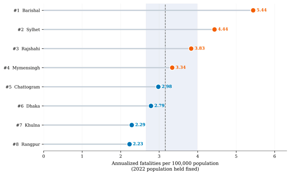
Figure 4.
Bootstrap mean monthly fatality rates by division with 95% percentile confidence intervals based on 5,000 resamples.
Figure 4.
Bootstrap mean monthly fatality rates by division with 95% percentile confidence intervals based on 5,000 resamples.
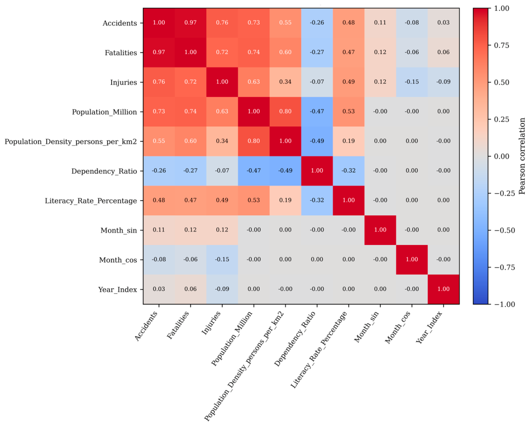
Figure 5.
Singular-value spectrum of the fatality-model design matrix.
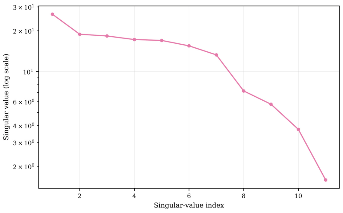
Figure 6.
Condition number of the ridge-stabilized normal-equation matrix over the regularization path.
Figure 6.
Condition number of the ridge-stabilized normal-equation matrix over the regularization path.
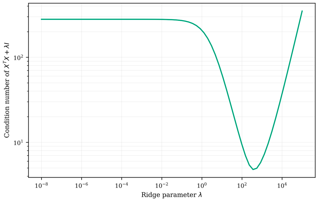
Figure 7.
Vandermonde condition number by polynomial degree before and after scaling the time coordinate to [-1,1].
Figure 7.
Vandermonde condition number by polynomial degree before and after scaling the time coordinate to [-1,1].
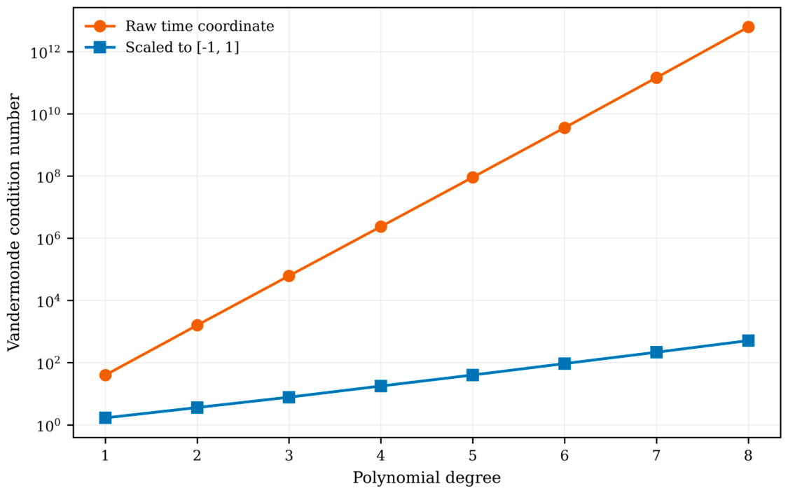
Figure 8.
Observed national fatalities with natural cubic-spline interpolation, LOOCV-selected cubic polynomial, and Savitzky-Golay smoothed trend.
Figure 8.
Observed national fatalities with natural cubic-spline interpolation, LOOCV-selected cubic polynomial, and Savitzky-Golay smoothed trend.
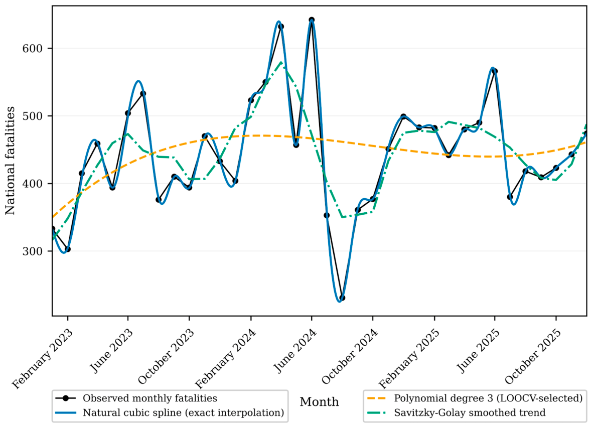
Figure 9.
First-derivative estimates of national monthly fatalities from exact cubic splines, second-order finite differences, and Savitzky-Golay smoothing.
Figure 9.
First-derivative estimates of national monthly fatalities from exact cubic splines, second-order finite differences, and Savitzky-Golay smoothing.
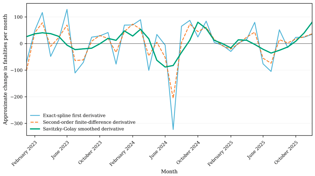
Figure 10.
Normalized RMSE across the statistical and machine-learning model library under leave-one-year-out validation.
Figure 10.
Normalized RMSE across the statistical and machine-learning model library under leave-one-year-out validation.
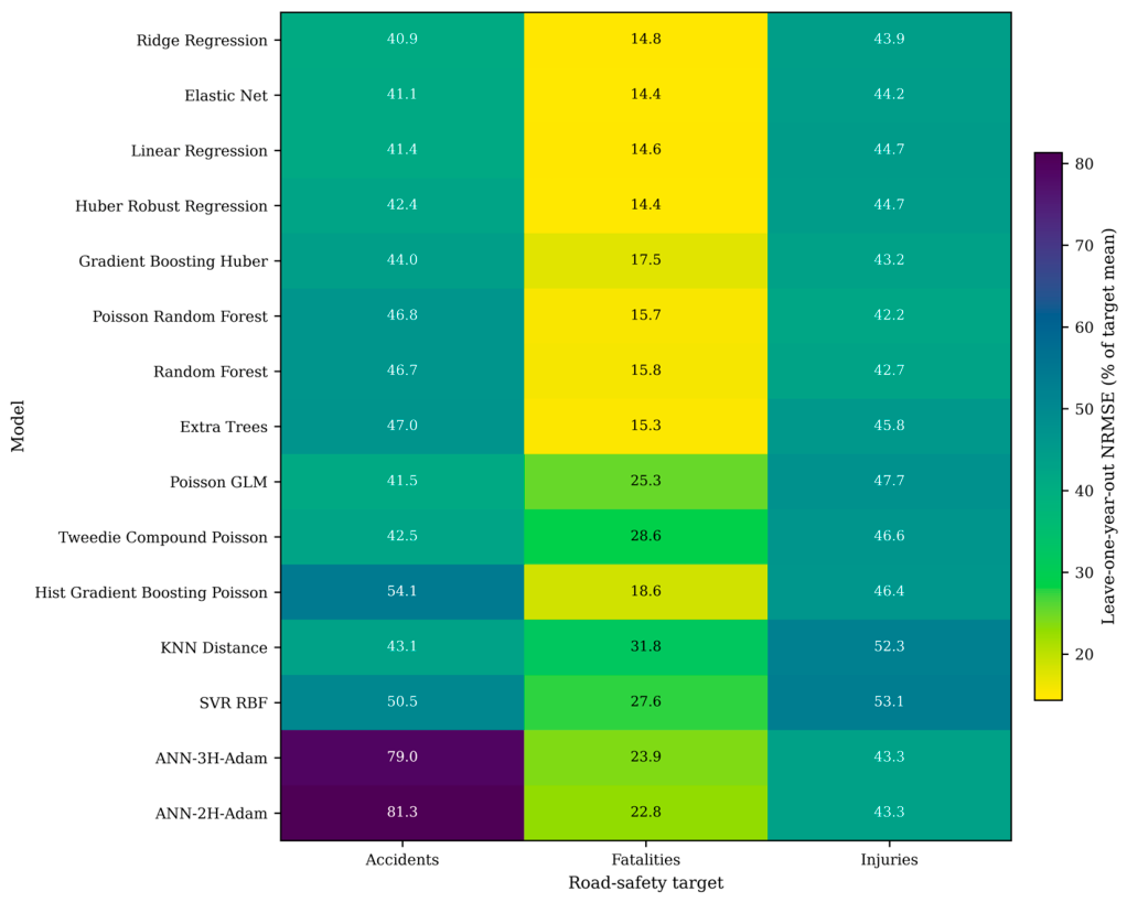
Figure 11.
Observed versus leave-one-year-out predicted accident counts for the best-performing Ridge regression model.
Figure 11.
Observed versus leave-one-year-out predicted accident counts for the best-performing Ridge regression model.
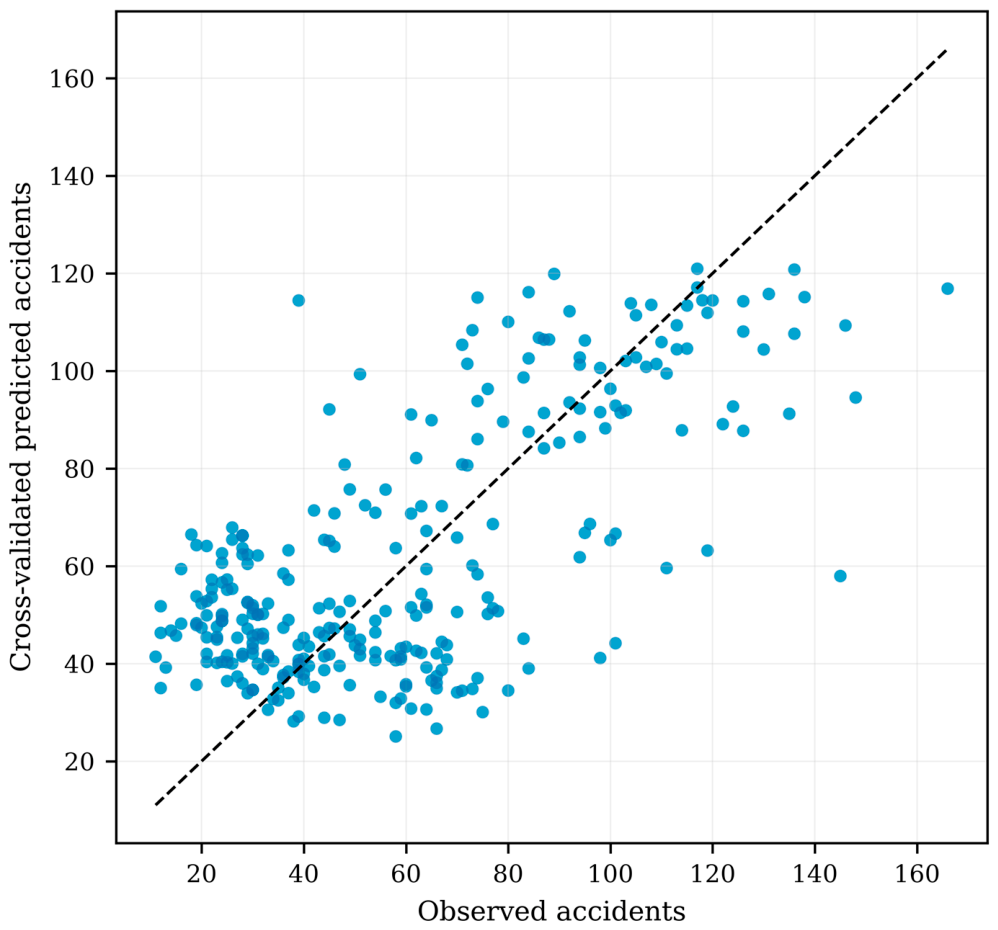
Figure 12.
Observed versus leave-one-year-out predicted fatalities for the best-performing Huber robust regression model.
Figure 12.
Observed versus leave-one-year-out predicted fatalities for the best-performing Huber robust regression model.
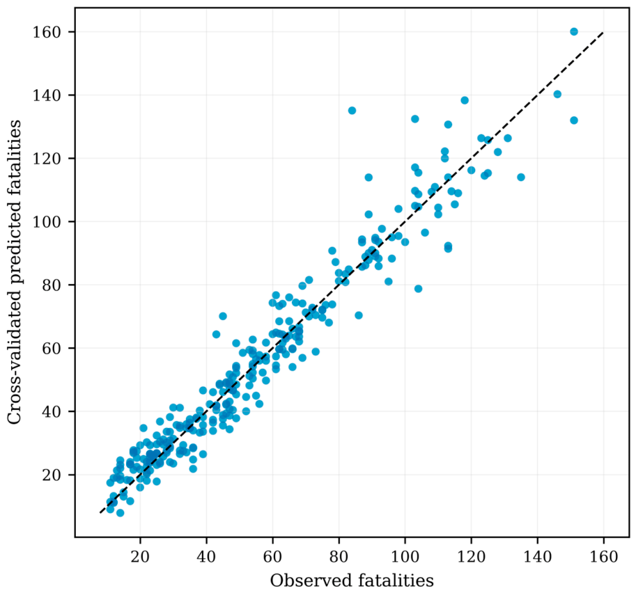
Figure 13.
Observed versus leave-one-year-out predicted injuries for the best-performing Poisson random forest model.
Figure 13.
Observed versus leave-one-year-out predicted injuries for the best-performing Poisson random forest model.
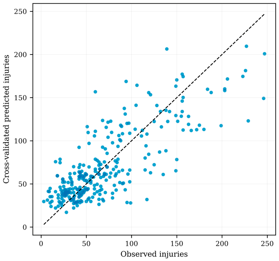
Figure 14.
Vehicle-type fatalities per 100 recorded vehicles using matched, non-missing records with positive denominators.
Figure 14.
Vehicle-type fatalities per 100 recorded vehicles using matched, non-missing records with positive denominators.
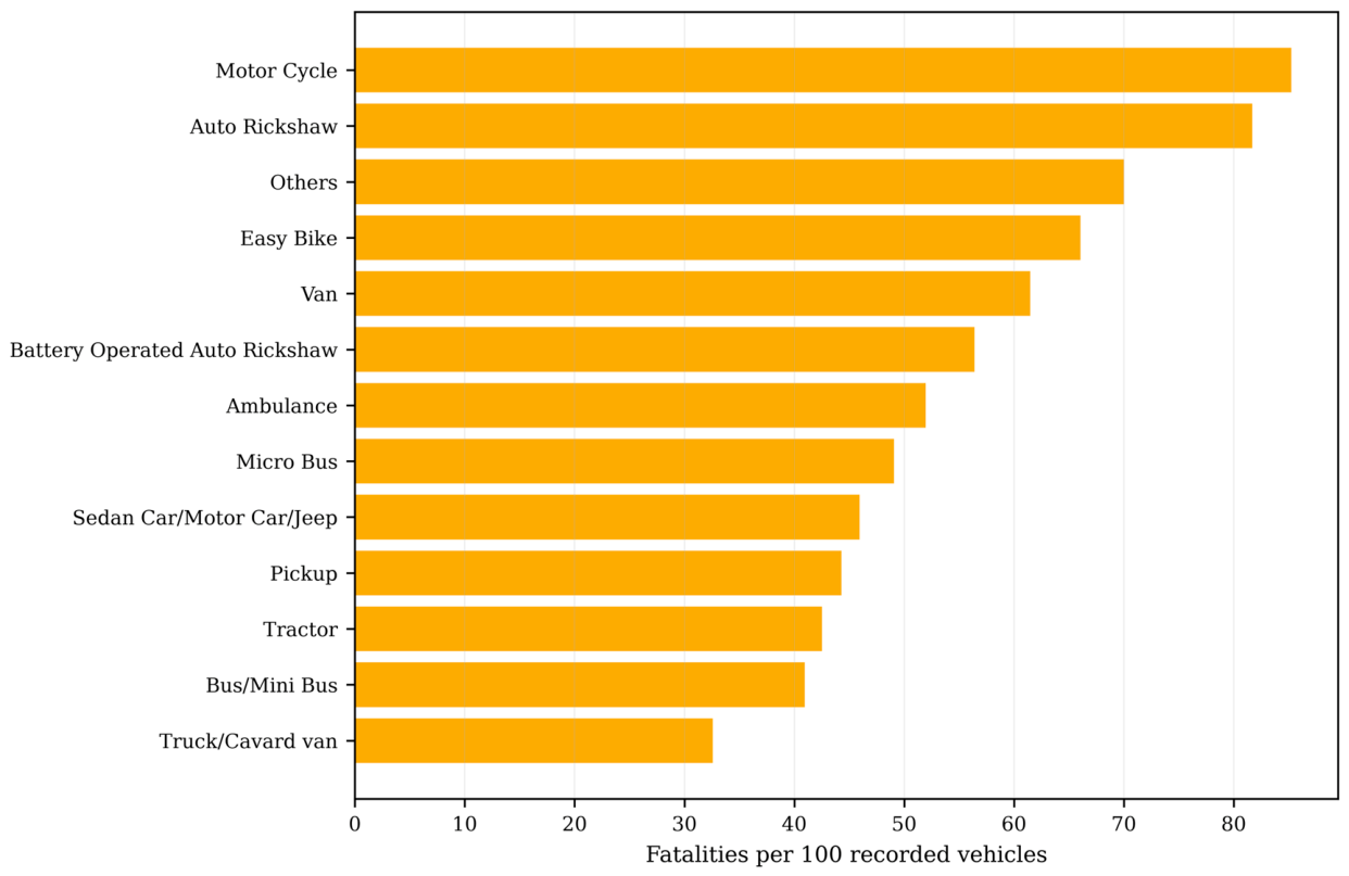
Figure 15.
Division-by-vehicle-type heat map of fatalities per 100 recorded vehicles for matched positive-denominator records.
Figure 15.
Division-by-vehicle-type heat map of fatalities per 100 recorded vehicles for matched positive-denominator records.
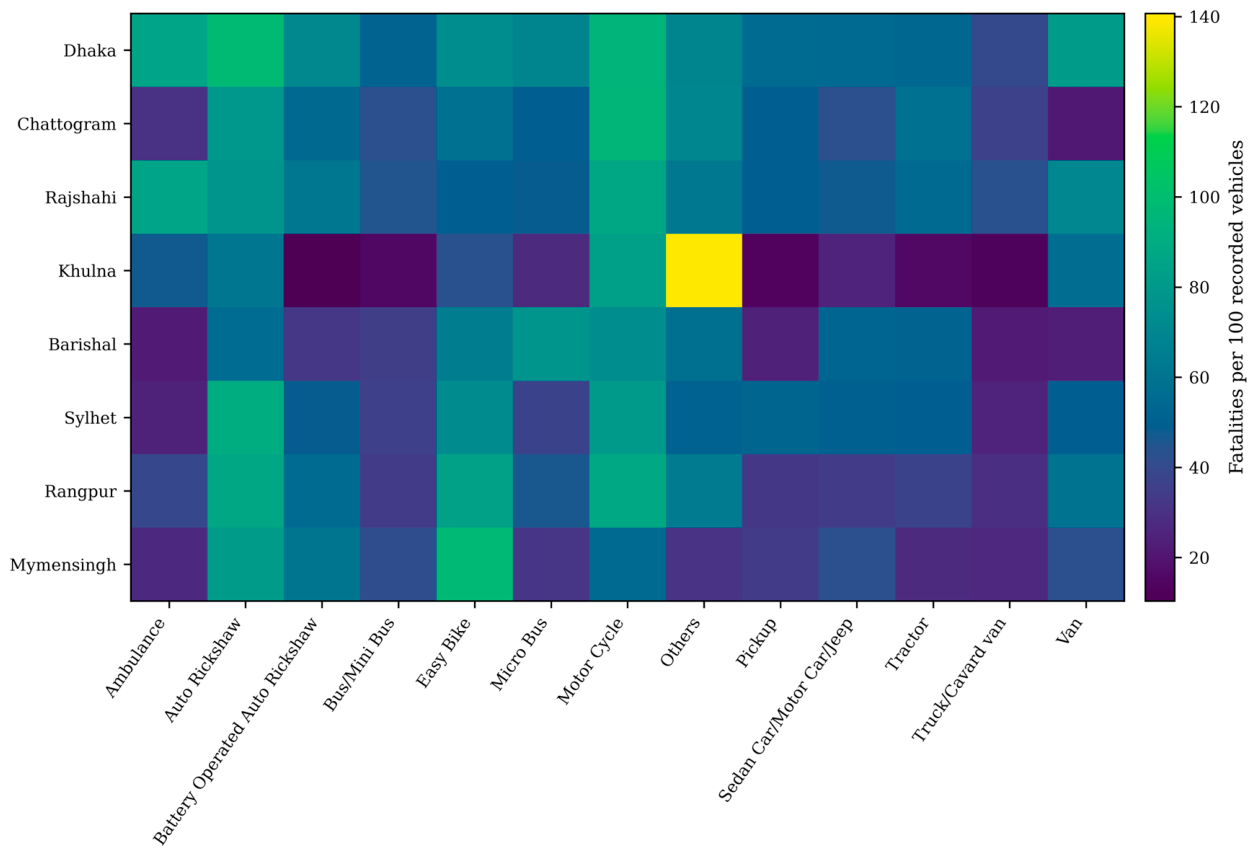
Figure 16.
Observed versus fitted fatalities for numerically optimized Poisson and NB2 conditional count models.
Figure 16.
Observed versus fitted fatalities for numerically optimized Poisson and NB2 conditional count models.
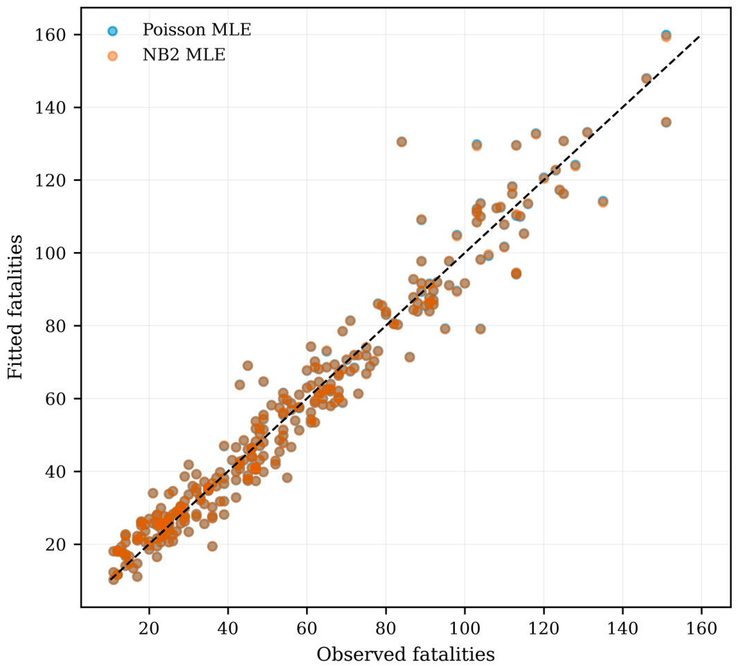
Figure 17.
Local-linear-trend Kalman filter and RTS smoother estimate of the latent national fatality level with state uncertainty.
Figure 17.
Local-linear-trend Kalman filter and RTS smoother estimate of the latent national fatality level with state uncertainty.
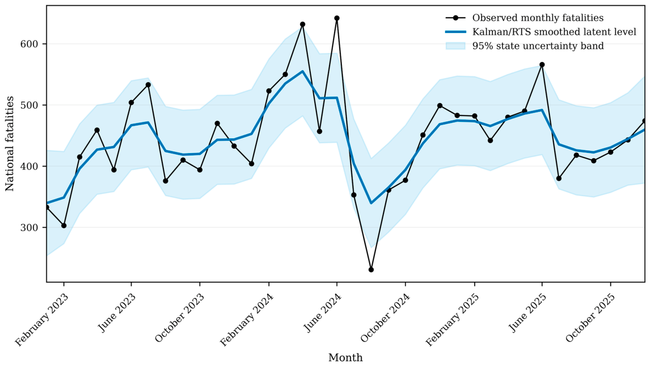
Figure 18.
Detrended Fourier power spectrum of national monthly fatalities, highlighting the dominant 12-month annual component.
Figure 18.
Detrended Fourier power spectrum of national monthly fatalities, highlighting the dominant 12-month annual component.
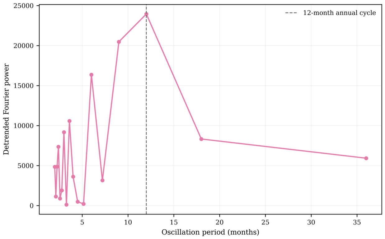
Figure 19.
National fatality series reconstructed from the fitted linear trend and four strongest Fourier harmonics.
Figure 19.
National fatality series reconstructed from the fitted linear trend and four strongest Fourier harmonics.
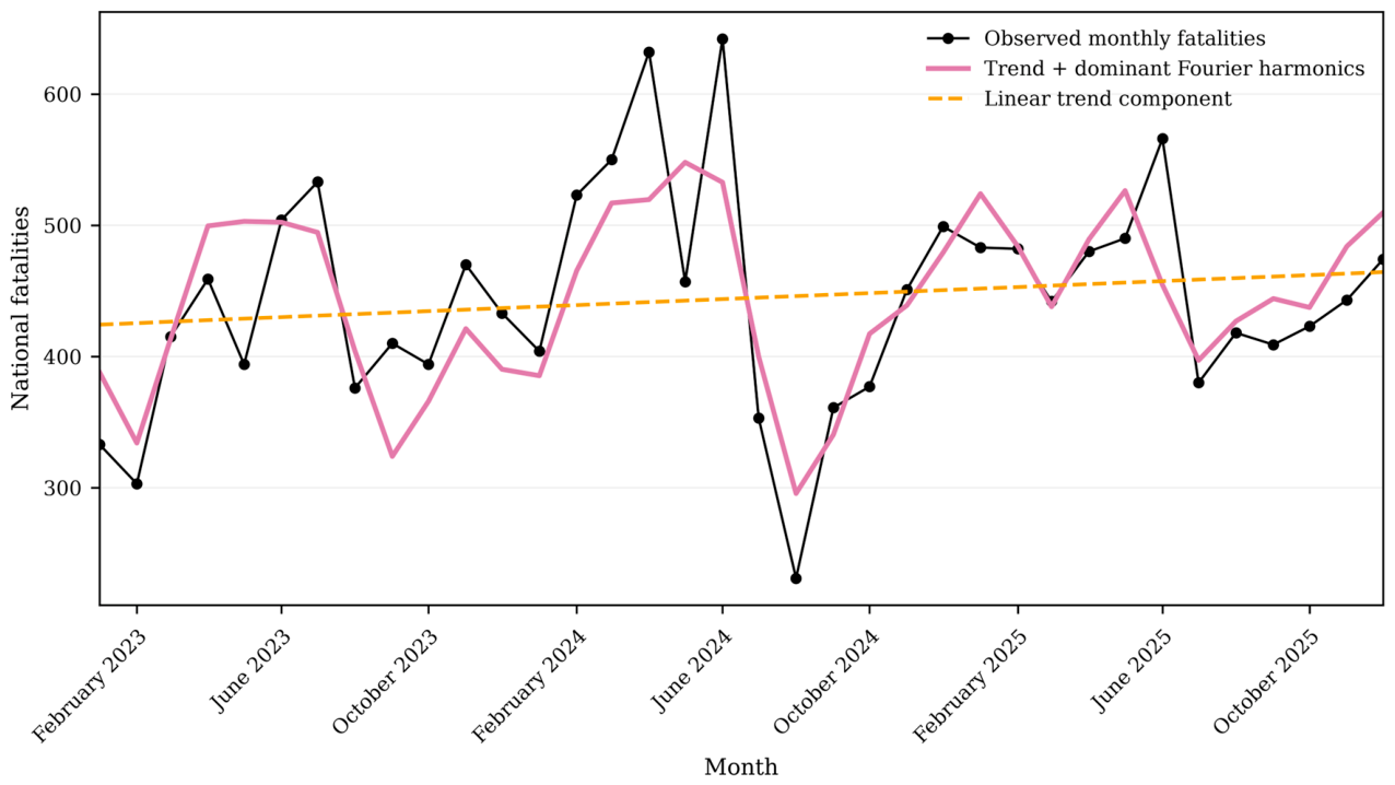
Figure 20.
Generalized cross-validation and coefficient-system conditioning over the Tikhonov regularization path.
Figure 20.
Generalized cross-validation and coefficient-system conditioning over the Tikhonov regularization path.
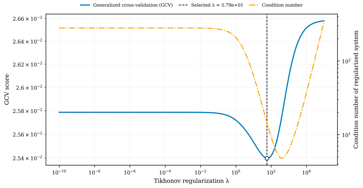
Figure 21.
Training-loss histories for the ANN-3H-Adam models with 128-64-32 ReLU hidden layers.
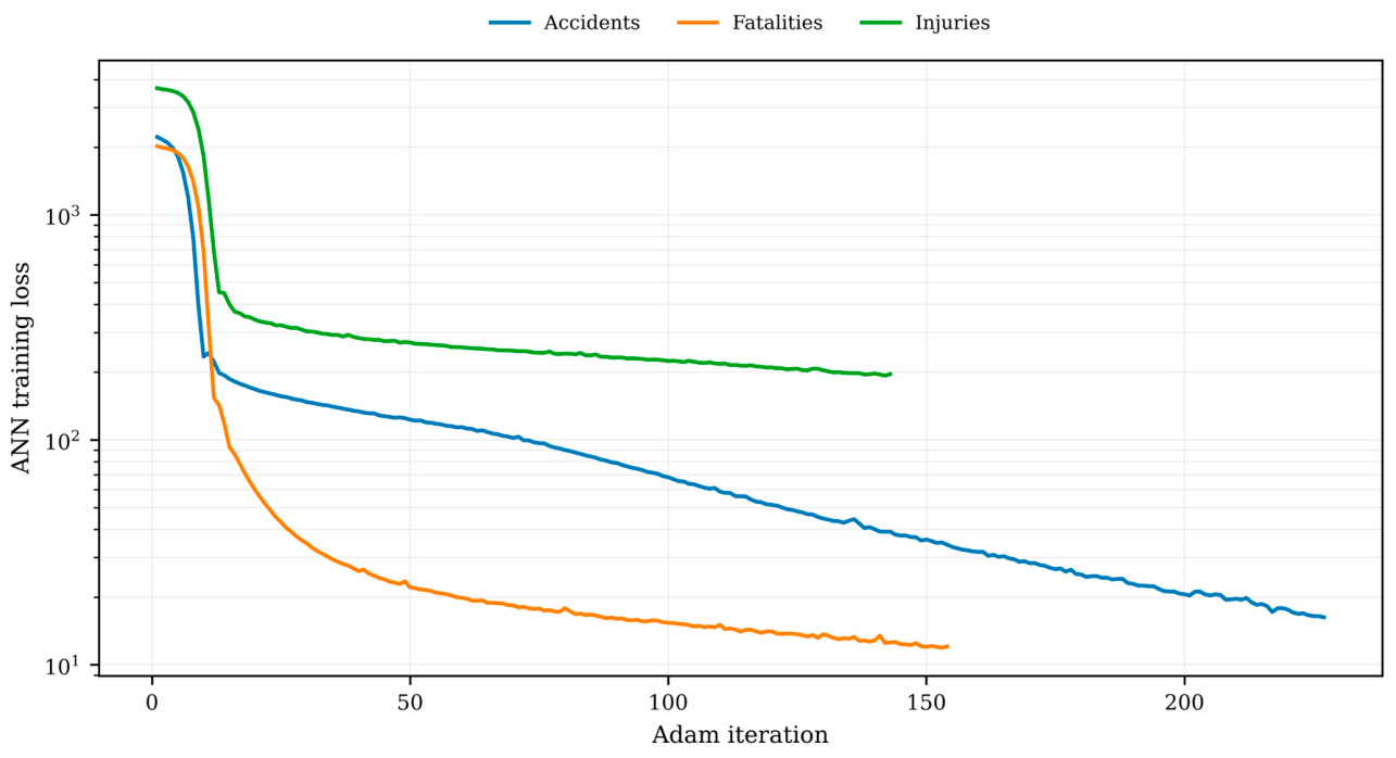
Figure 22.
Observed versus leave-one-year-out ANN-3H-Adam predictions for accidents.
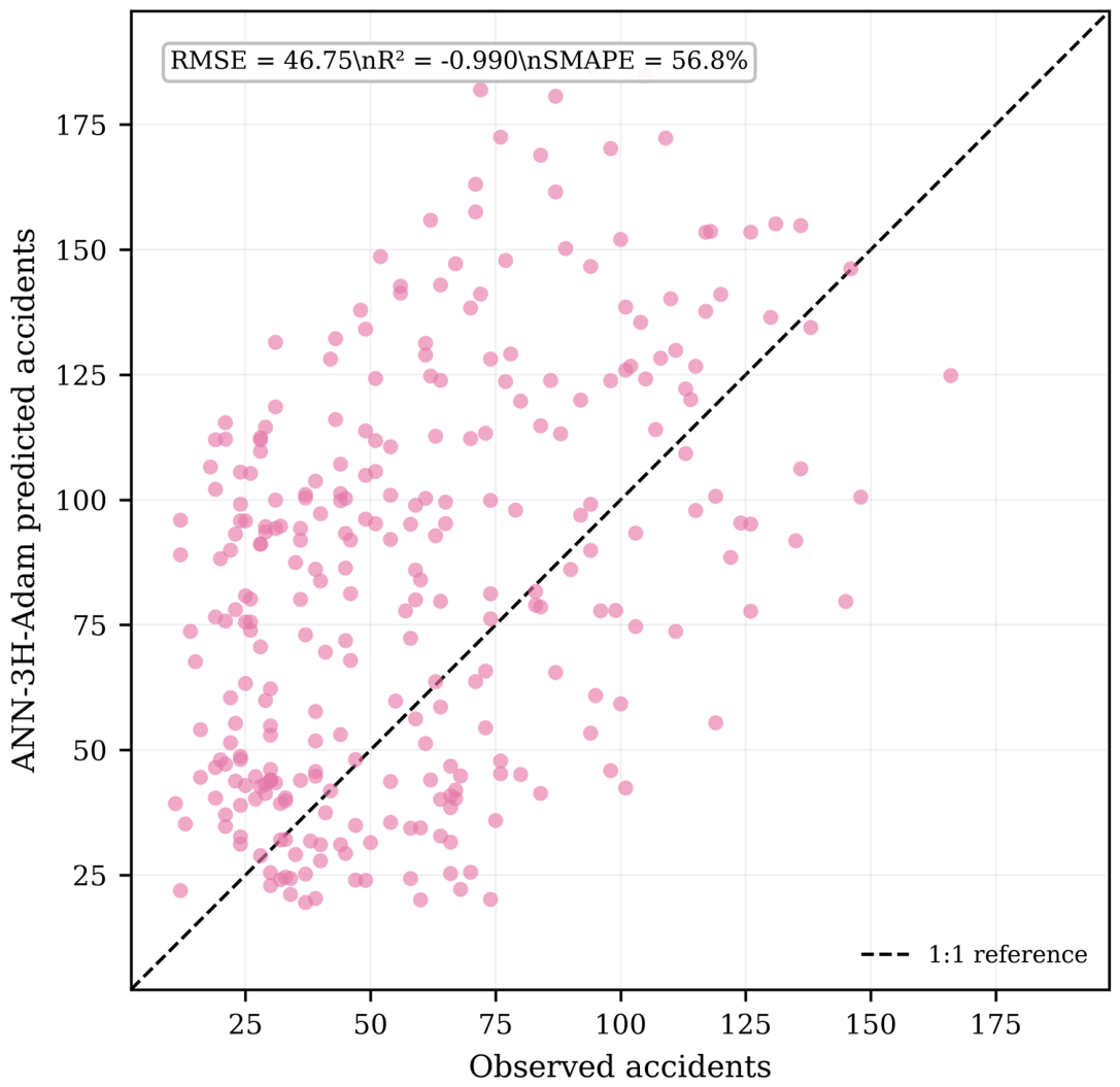
Figure 23.
Observed versus leave-one-year-out ANN-3H-Adam predictions for fatalities.
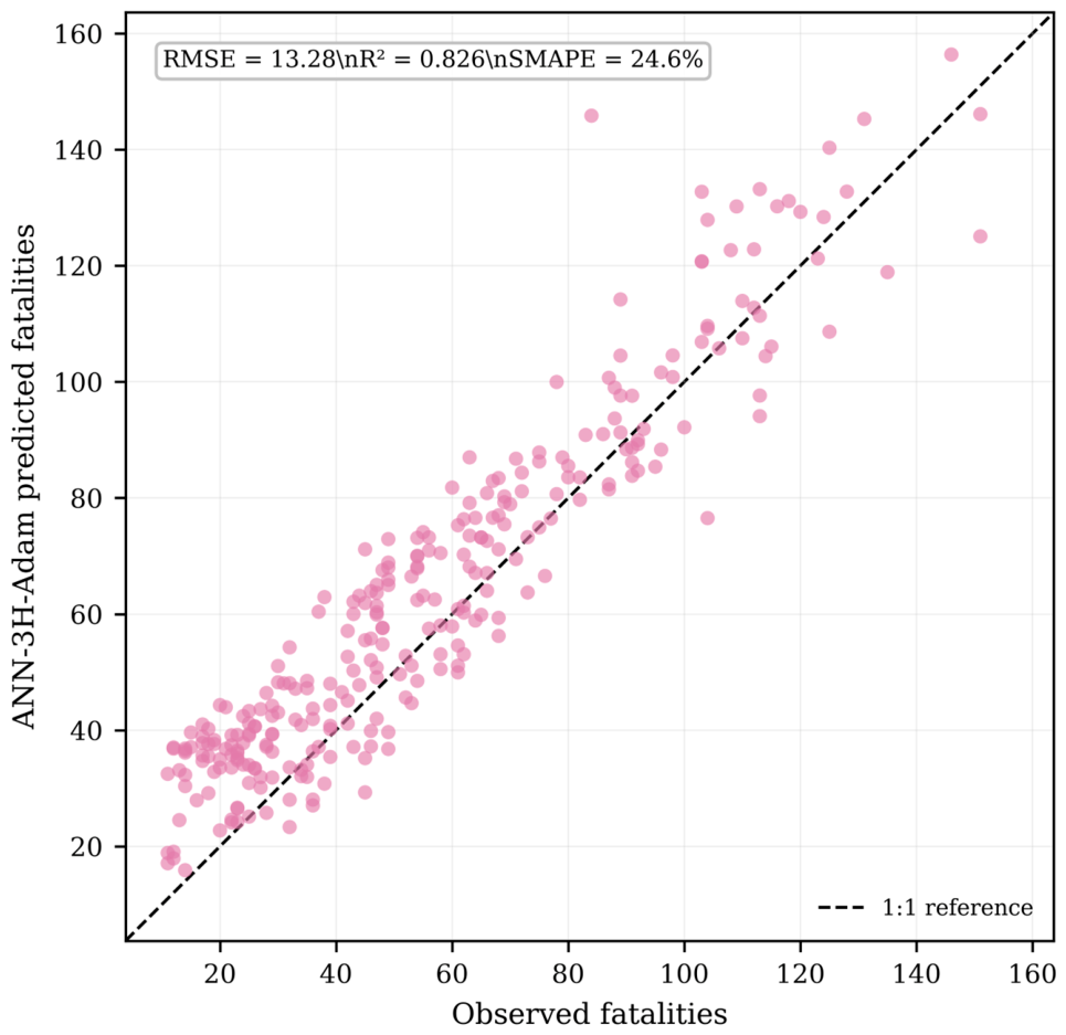
Figure 24.
Observed versus leave-one-year-out ANN-3H-Adam predictions for injuries.
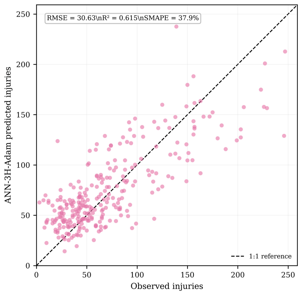
Figure 25.
Best numerical method versus best statistical/machine-learning model for each outcome under identical leave-one-year-out folds. Lower NRMSE is better.
Figure 25.
Best numerical method versus best statistical/machine-learning model for each outcome under identical leave-one-year-out folds. Lower NRMSE is better.
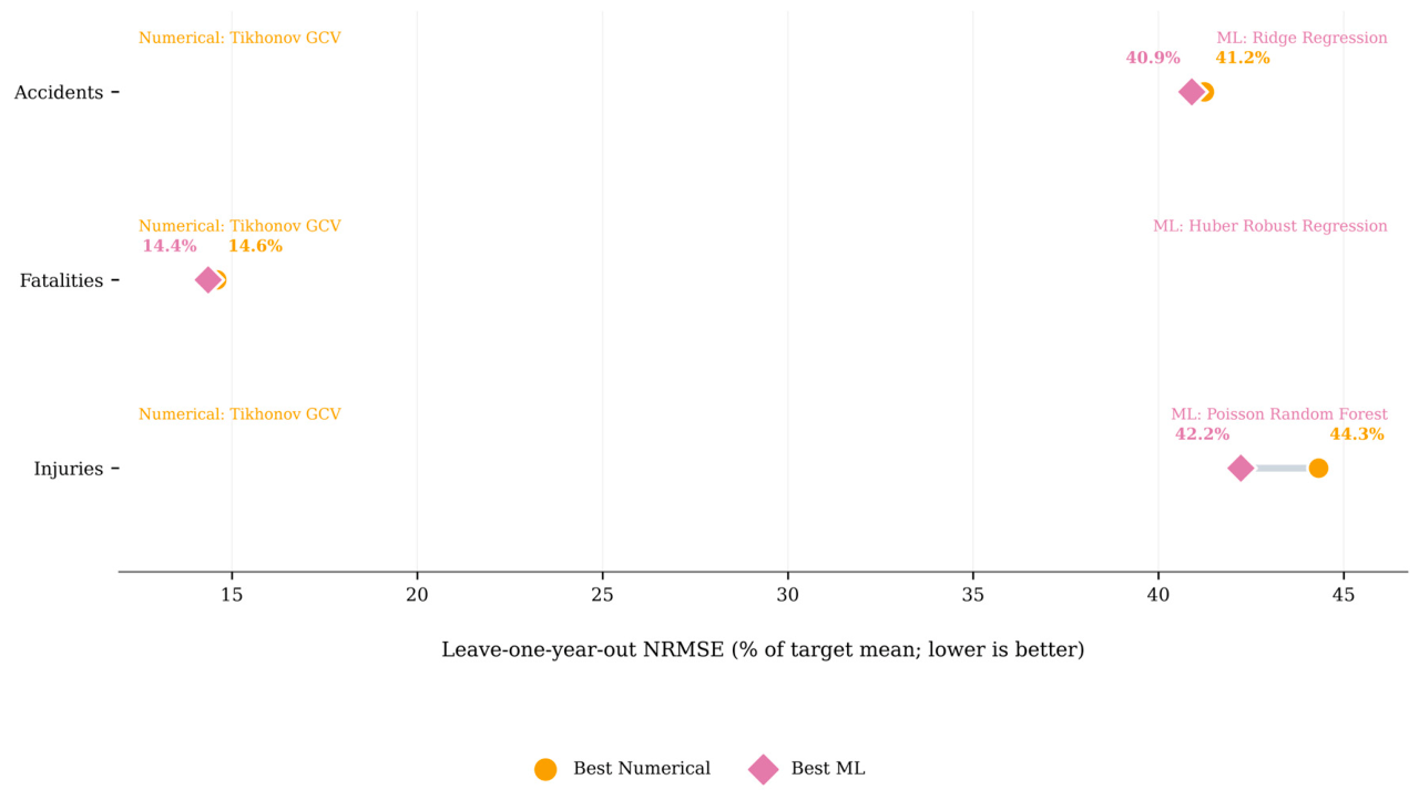
Figure 26.
Annual observed totals and out-of-time predictions from the best numerical and best statistical/machine-learning model for accidents, fatalities, and injuries.
Figure 26.
Annual observed totals and out-of-time predictions from the best numerical and best statistical/machine-learning model for accidents, fatalities, and injuries.
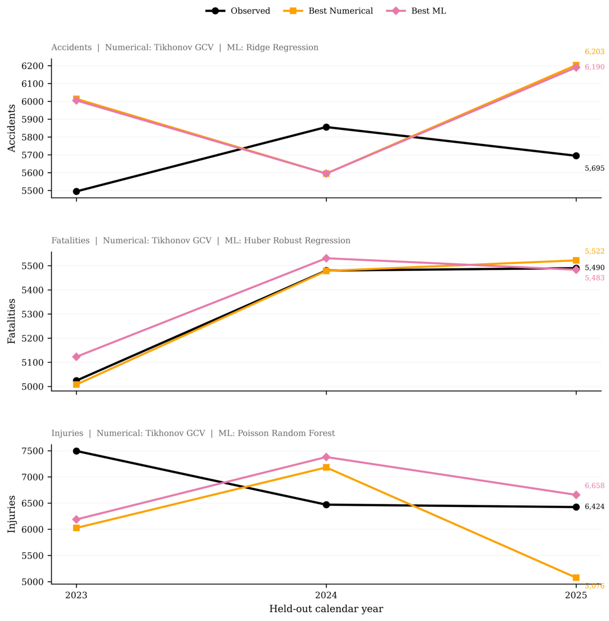
Figure 27.
Combined NRMSE heat map for numerical solvers and the complete statistical/machine-learning model library. Lower values indicate better out-of-time performance.
Figure 27.
Combined NRMSE heat map for numerical solvers and the complete statistical/machine-learning model library. Lower values indicate better out-of-time performance.
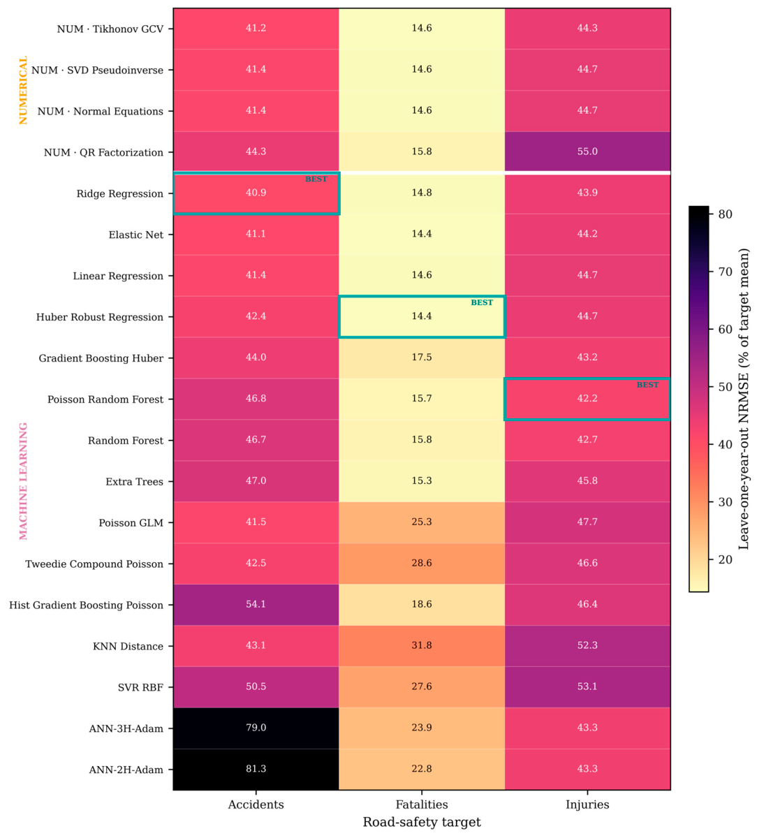

Table 1.
Study datasets, completeness, and analytical roles.
| Dataset | Rows | Missing cells (%) | Analytical role |
| Population (2022) | 9 | 0.000 | Population exposure and division context |
| Main accident panel | 288 | 0.000 | Division-month accidents, fatalities, and injuries |
| Vehicle fatalities | 3743 | 1.850 | Vehicle-type fatality numerator |
| Vehicle counts | 3744 | 1.230 | Vehicle-type recorded-vehicle denominator |
Note: The population file contains eight division records plus a national total row; only division-level records are used as denominators. Missing vehicle cells are retained as missing rather than recoded to zero.
Table 2.
Predictive model library and principal settings.
| Model | Key setting | Role |
| Linear regression | OLS | Closed-form/least-squares baseline |
| Ridge regression | α=10 | L2 regularization |
| Elastic Net | α=0.03; l1_ratio=0.35 | Mixed L1/L2 penalty |
| Huber robust regression | ε=1.35; α=0.0005 | Robust residual loss |
| Poisson GLM | α=0.10; log link | Count-aware GLM |
| Tweedie GLM | power=1.5; α=0.10; log link | Compound-Poisson variance |
| SVR-RBF | C=30; ε=0.10; gamma=scale | RBF kernel |
| KNN distance | k=9; inverse-distance weights; p=2 | Local nonlinear regression |
| ANN-2H-Adam | 64-32 ReLU; batch=32; lr=1.5e-3 | Early stopping; L2=1e-3 |
| ANN-3H-Adam | 128-64-32 ReLU; batch=32; lr=1.0e-3 | Early stopping; L2=1e-3 |
| Random forest | 350 trees; min leaf=2; max_features=0.85 | Squared-error trees |
| Poisson random forest | 350 trees; Poisson criterion | Count-aware tree split criterion |
| Extra Trees | 400 trees; min leaf=2; max_features=0.90 | Highly randomized trees |
| Gradient boosting | 500 trees; Huber loss; lr=0.035 | Depth=2; min leaf=3 |
| Histogram gradient boosting | Poisson loss; 650 iterations; lr=0.04 | max leaves=15; L2=1.0 |
Note: Every candidate uses the same target-specific preprocessing and the same leave-one-year-out folds. ANN models are implemented with scikit-learn MLPRegressor and Adam.
Table 3.
Annual national road-accident burden and year-on-year change.
| Year | Accidents | Fatalities | Injuries | Accident YoY (%) | Fatality YoY (%) | Injury YoY (%) |
| 2023 | 5,495 | 5,024 | 7,495 | — | — | — |
| 2024 | 5,856 | 5,480 | 6,470 | 6.57 | 9.08 | -13.68 |
| 2025 | 5,695 | 5,490 | 6,424 | -2.75 | 0.18 | -0.71 |
Table 4.
Division-level population-adjusted fatality burden with bootstrap uncertainty.
| Division | Annualized fatalities/100k | Mean monthly fatalities/100k | 95% CI lower | 95% CI upper |
| Barishal | 5.44 | 0.453 | 0.383 | 0.528 |
| Sylhet | 4.44 | 0.370 | 0.317 | 0.424 |
| Rajshahi | 3.83 | 0.319 | 0.290 | 0.348 |
| Mymensingh | 3.34 | 0.278 | 0.244 | 0.314 |
| Chattogram | 2.98 | 0.248 | 0.228 | 0.269 |
| Dhaka | 2.79 | 0.232 | 0.216 | 0.248 |
| Khulna | 2.29 | 0.191 | 0.158 | 0.225 |
| Rangpur | 2.23 | 0.186 | 0.161 | 0.213 |
Note: Annualized rates use the fixed 2022 population denominator. Confidence intervals are percentile intervals from 5,000 bootstrap resamples of monthly division-specific rates.
Table 5.
Core numerical-conditioning diagnostics.
| Diagnostic | Value | Interpretation |
| Inferential design rank | 11/11 | Full rank |
| Largest singular value | 26.517 | Dominant design direction |
| Smallest singular value | 1.585 | No near-null terminal direction |
| κ₂(X) | 16.73 | Moderate conditioning |
| κ₂(XᵀX) | 279.97 | Normal equations amplify conditioning |
| Selected polynomial degree | 3 | Minimum LOOCV RMSE |
| Degree-3 raw-time κ(V) | 6.21e+04 | Severely ill-conditioned |
| Degree-3 scaled-time κ(V) | 7.77 | Stable after scaling |
Note: Condition numbers use the 2-norm. The normal-equation condition number is approximately the square of κ₂(X) for a full-rank design.
Table 6.
Selected numerical time-series diagnostics for national fatalities.
| Diagnostic | Value | Interpretation |
| Selected polynomial degree | 3 | Minimum LOOCV RMSE |
| Cubic in-sample RMSE | 78.13 | Approximation error |
| Cubic LOOCV RMSE | 84.80 | Out-of-sample degree criterion |
| Minimum spline derivative | ≈ -323 fatalities/month | Sharp mid-2024 decline |
| Minimum finite-difference derivative | ≈ -206 fatalities/month | Less extreme local change |
| Minimum Savitzky-Golay derivative | ≈ -88 fatalities/month | Smoothed trend velocity |
| Dominant Fourier period | 12 months | Annual recurrence |
| Dominant Fourier power | 23,947 | Strongest non-zero component |
| Dominant Fourier amplitude | 51.58 | Annual harmonic amplitude |
| Four-harmonic reconstruction RMSE | 52.46 | Trend + dominant harmonics |
| Four-harmonic reconstruction MAE | 41.49 | Absolute reconstruction error |
Source: authors' numerical analysis of the 36-month national fatality series.
Table 7.
Best statistical/machine-learning model for each outcome under leave-one-year-out validation.
Table 7.
Best statistical/machine-learning model for each outcome under leave-one-year-out validation.
| Target | Best model | MAE | RMSE | R² | SMAPE (%) | NRMSE (%) | Spearman ρ |
| Accidents | Ridge Regression | 19.61 | 24.20 | 0.467 | 38.05 | 40.89 | 0.512 |
| Fatalities | Huber Robust Regression | 5.63 | 7.97 | 0.937 | 12.47 | 14.35 | 0.971 |
| Injuries | Poisson Random Forest | 22.64 | 29.89 | 0.633 | 36.21 | 42.22 | 0.723 |
Note: All predictions are out-of-fold under leave-one-year-out validation.
Table 8.
Highest vehicle-type exposure-style fatality ratios.
| Vehicle type | Fatalities | Recorded vehicles | Fatalities/100 recorded vehicles |
| Motor Cycle | 4,650 | 5,455 | 85.24 |
| Auto Rickshaw | 1,311 | 1,605 | 81.68 |
| Others | 2,787 | 3,981 | 70.01 |
| Easy Bike | 506 | 766 | 66.06 |
| Van | 434 | 706 | 61.47 |
| Battery Operated Auto Rickshaw | 630 | 1,117 | 56.40 |
| Ambulance | 66 | 127 | 51.97 |
| Micro Bus | 265 | 540 | 49.07 |
Note: Ratios use only matched, non-missing records with positive recorded-vehicle denominators. They are screening indicators, not registered-fleet or vehicle-distance fatality rates.
Table 9.
Numerically optimized Poisson and NB2 fatality-count model fit.
| Model | Log-likelihood | AIC | BIC | NB2 α | Pearson dispersion |
| Poisson MLE | -953.50 | 1928.99 | 1969.28 | — | 0.969 |
| Negative Binomial NB2 MLE | -953.55 | 1931.09 | 1975.05 | 7.33e-05 | — |
Note: Accident count enters as a log-offset. Lower AIC/BIC favors the simpler Poisson model.
Table 10.
Poisson fatality-model incidence-rate ratios.
| Term | IRR | 95% CI lower | 95% CI upper | p-value | Sig. |
| Year Index | 1.019 | 1.003 | 1.035 | 0.019 | * |
| Month sin | 1.011 | 0.974 | 1.050 | 0.553 | |
| Month cos | 1.032 | 0.994 | 1.072 | 0.104 | |
| Population Million | 0.975 | 0.943 | 1.007 | 0.129 | |
| Population density | 1.052 | 1.022 | 1.083 | <0.001 | *** |
| Dependency Ratio | 1.018 | 0.998 | 1.039 | 0.086 | |
| Literacy Rate Percentage | 0.998 | 0.975 | 1.022 | 0.859 |
Note: Continuous covariates are standardized and accident count enters as a log-offset. Significance codes: * p<0.05; ** p<0.01; *** p<0.001.
Table 11.
Best numerical versus best statistical/machine-learning NRMSE under the same leave-one-year-out folds.
Table 11.
Best numerical versus best statistical/machine-learning NRMSE under the same leave-one-year-out folds.
| Target | Best numerical | NRMSE (%) | Best ML/statistical | NRMSE (%) | Absolute gap (pp) |
| Accidents | Tikhonov GCV | 41.2 | Ridge Regression | 40.9 | 0.3 |
| Fatalities | Tikhonov GCV | 14.6 | Huber Robust Regression | 14.4 | 0.2 |
| Injuries | Tikhonov GCV | 44.3 | Poisson Random Forest | 42.2 | 2.1 |
Note: Lower NRMSE is better. Percentage-point gaps are computed from the displayed one-decimal NRMSE values.
Table 12.
Complete NRMSE landscape for numerical and statistical/machine-learning models.
| Model | Family | Accidents (%) | Fatalities (%) | Injuries (%) |
| Tikhonov GCV | Numerical | 41.2 | 14.6 | 44.3 |
| SVD Pseudoinverse | Numerical | 41.4 | 14.6 | 44.7 |
| Normal Equations | Numerical | 41.4 | 14.6 | 44.7 |
| QR Factorization | Numerical | 44.3 | 15.8 | 55.0 |
| Ridge Regression | ML/statistical | 40.9 | 14.8 | 43.9 |
| Elastic Net | ML/statistical | 41.1 | 14.4 | 44.2 |
| Linear Regression | ML/statistical | 41.4 | 14.6 | 44.7 |
| Huber Robust Regression | ML/statistical | 42.4 | 14.4 | 44.7 |
| Gradient Boosting Huber | ML/statistical | 44.0 | 17.5 | 43.2 |
| Poisson Random Forest | ML/statistical | 46.8 | 15.7 | 42.2 |
| Random Forest | ML/statistical | 46.7 | 15.8 | 42.7 |
| Extra Trees | ML/statistical | 47.0 | 15.3 | 45.8 |
| Poisson GLM | ML/statistical | 41.5 | 25.3 | 47.7 |
| Tweedie Compound Poisson | ML/statistical | 42.5 | 28.6 | 46.6 |
| Hist Gradient Boosting Poisson | ML/statistical | 54.1 | 18.6 | 46.4 |
| KNN Distance | ML/statistical | 43.1 | 31.8 | 52.3 |
| SVR RBF | ML/statistical | 50.5 | 27.6 | 53.1 |
| ANN-3H-Adam | ML/statistical | 79.0 | 23.9 | 43.3 |
| ANN-2H-Adam | ML/statistical | 81.3 | 22.8 | 43.3 |
Note: Values are leave-one-year-out NRMSE. Lower values indicate better out-of-time predictive performance.
Disclaimer/Publisher’s Note: The statements, opinions and data contained in all publications are solely those of the individual author(s) and contributor(s) and not of MDPI and/or the editor(s). MDPI and/or the editor(s) disclaim responsibility for any injury to people or property resulting from any ideas, methods, instructions or products referred to in the content. |
© 2026 by the authors. Licensee MDPI, Basel, Switzerland. This article is an open access article distributed under the terms and conditions of the Creative Commons Attribution (CC BY) license.
Copyright: This open access article is published under a Creative Commons CC BY 4.0 license, which permit the free download, distribution, and reuse, provided that the author and preprint are cited in any reuse.