

Submitted:
08 September 2026
Posted:
09 September 2026
You are already at the latest version
Abstract
Harmonic distortion at low-voltage points of common coupling (PCCs) is an operational concern as power-electronics-interfaced loads proliferate across distribution networks. This study investigates whether power-quality index telemetry, rather than continuous waveform measurements, can support probabilistic forecasting of voltage total harmonic distortion (UTHD) and its margin to an IEEE 519-2022 reference boundary. A telemetry-first framework is developed using exported power-quality indices at 10-min intervals. A multi-output histogram-based gradient-boosting regressor forecasts per-phase UTHD at 10-, 30-, 60-, and 120-min horizons and is benchmarked against six baseline methods. Adaptive split-conformal calibration is applied to construct prediction intervals, with finite-sample marginal coverage interpreted under the exchangeability assumption. Using an 11,088-sample data-centre dataset spanning 77 days, the primary phase-B target achieves a mean absolute error of 0.274 percentage points at the 10-min horizon, representing a 20% reduction relative to persistence (p < 10−4). Frozen-model transfer to two independently instrumented external sites is also evaluated, with target-site conformal recalibration using labelled calibration subsets. The results provide empirical evidence that index-only telemetry can support multi-horizon UTHD forecasting with uncertainty intervals, while distributional shift provides a useful diagnostic for cross-site transfer.
Keywords:
harmonic distortion
; conformal prediction
; gradient boosting
; IEC 61000-4-30
; IEEE 519-2022
; low-voltage distribution
; power quality
; probabilistic forecasting
; telemetry-first analytics
; covariate shift
1. Introduction
The proliferation of power-electronics-interfaced loads at the low-voltage tier of distribution networks has made harmonic distortion a routine operational concern. Grid-connected photovoltaic inverters, electric-vehicle (EV) chargers, variable-speed drives, and single-phase switching loads inject non-sinusoidal currents that propagate as voltage distortion at every connected node, producing elevated transformer losses, accelerated insulation ageing, protective-relay mis-operation, and cable derating near the thermal limit [1,2]. Taghvaie et al. [3] review the increasingly complex harmonic characteristics and estimation challenges in modern power networks, while Li et al. [4] and Kazemtarghi et al. [5] document power-quality challenges associated with distributed photovoltaic and EV charging integration.
IEEE 519-2022 [6] specifies voltage harmonic-distortion limits at the PCC, including an 8% total-voltage-distortion reference limit for systems at or below 1 kV. IEC 61000-4-30 [7] and IEC 61000-4-7 [8] define the measurement and aggregation procedures used to obtain power-quality indices. In this study, these aggregated quantities form the available telemetry modality. Methods that require waveform-level inputs [10,11,12,13] cannot be directly applied when only aggregated index telemetry is available. The present work therefore evaluates forecasting and uncertainty quantification using the retained index measurements rather than continuous waveforms.
Compliance-oriented monitoring is most useful when it provides an estimate of the remaining distance to a reference boundary before a potential exceedance. The available datasets contain no IEEE 519 exceedance events. Consequently, the present evaluation focuses on probabilistic UTHD and compliance-margin forecasting under the observed operating conditions rather than on validated exceedance-event detection. The absence of observed exceedances is therefore treated as a characteristic of the available data, not as evidence that exceedance detection has been validated.
The study addresses four methodological gaps identified in the reviewed literature. First, harmonic forecasting studies use different targets, input modalities, and uncertainty constructions [13,14,16,18]. Second, the present study evaluates multiple forecast horizons on a common operational telemetry dataset using a fixed baseline suite and statistical comparison. Third, the proposed uncertainty layer uses split conformal calibration rather than a parametric residual model, while recognising that the formal finite-sample guarantee depends on the usual exchangeability assumption [33,34]. Fourth, the study evaluates frozen cross-site transfer and quantifies feature-distribution shift rather than retraining a separate point predictor at each site.
An earlier conference pilot [17] established the feasibility of telemetry-first harmonic-state detection on a single 11-hour record at 4-second cadence; this journal paper extends that pilot to IEC 61000-4-30 10-min aggregation, distribution-free probabilistic intervals, three-site external validation, and full computational-footprint reporting.
The contributions are fourfold. (C1) A telemetry-native framework is formulated to forecast voltage UTHD and compliance margin from IEC 61000-4-30 index exports without waveform access. (C2) A multi-output HGBR produces 10-, 30-, 60-, and 120-min ahead per-phase UTHD forecasts and is compared with a fixed baseline suite using Diebold–Mariano tests and block-bootstrap confidence intervals. (C3) An adaptive split-conformal layer provides empirically calibrated prediction intervals, with the exchangeability condition and the observed coverage–width trade-off reported explicitly. (C4) Frozen-model cross-site transfer is evaluated on two independently instrumented external sites, with the point predictor kept fixed and the conformal layer recalibrated on a small labelled target subset; feature-distribution shift is quantified alongside predictive degradation.
The remainder of this paper is structured as follows. Section 2 surveys the related literature. Section 3 formalises the monitoring problem. Section 4 describes the proposed framework. Section 5 presents the experimental results. Section 6 provides discussion including limitations. Section 7 draws conclusions.
2. Related Work
2.1. Harmonic Standards and Measurement Framework
IEEE 519-2022 [6] sets compliance limits at the point of common coupling (PCC): UTHD to and individual voltage harmonic distortion to per order for systems at or below 1 kV. Current-side limits are expressed as total demand distortion (TDD) indexed by the short-circuit ratio and additionally require and , which are absent from standard telemetry exports, making voltage-centric targets the practical choice under index-only data retention.
IEC 61000-4-30 [7] defines Class A measurement and aggregation from a 200-ms basic measurement window through 3-second and 10-minute reporting intervals. IEC 61000-4-7 [8] specifies the underlying discrete Fourier analysis and the prevailing-phasor convention, which was documented in field measurements by Blanco et al. [13] and validated across a population of low-voltage sites by Meyer et al. [19]. IEC 61000-3-6 [20] defines the planning levels and emission-allocation principles by which network operators apportion harmonic budget among connected installations, translating a measured exceedance into a regulatory obligation with financial and operational consequences.
2.2. Power-Quality Monitoring: From Waveform to Telemetry
Power-quality analysis has historically been anchored to continuous high-rate waveform records, from which time-frequency features are derived through Fourier analysis, synchrosqueezed wavelet decompositions, and the Hilbert-Huang transform [1,2,21,22]. Comprehensive surveys confirm that the strongest discriminative methods depend most on this waveform modality and that the gap between laboratory and field performance is largely a data-availability issue [1,2]. Field-deployed analysers of the Metrel MI 550 Poly class [9] can export aggregated power-quality indices rather than continuous records. The present study therefore focuses on the forecasting problem that arises when such aggregated telemetry is the retained data modality.
The aggregated-index modality has also received direct analytical attention. Rodríguez-Pajarón et al. [24] forecast voltage harmonic distortion from smart-meter data in residential distribution networks, demonstrating the feasibility of learning harmonic behaviour from low-rate measurements. That work is complementary to the present framework, which uses exported power-quality indices as the sole input modality and forecasts multi-horizon voltage UTHD.
2.3. Machine Learning for Power-Quality Classification
Tree-based ensembles have also been applied to power-quality event detection and harmonic-source attribution. Mishra et al. [25] combine downsampling with an optimised random forest for islanding and non-islanding power-quality-event classification, while Mella et al. [26] use an ensemble classifier to determine harmonic contribution responsibility at microgrid PCCs. Sharma et al. [27] address reduced-sensor harmonic resonance detection and compensation, and Jaramillo et al. [28] study supervised identification of distributed-energy-resource electrical profiles in low-voltage networks.
Deep architectures remain prominent in power-quality disturbance classification. Vishwanath et al. [10] combine a synchrosqueezed wavelet transform with convolutional neural networks, Khetarpal et al. [11] use a deep convolutional autoencoder, and Chiam et al. [12] combine LSTM, wavelet, and attention mechanisms. Wang et al. [29] also investigate ensemble deep learning for automated power-quality-disturbance classification. These studies illustrate the maturity of waveform-oriented learning, while the present work targets index-only telemetry for forecasting.
2.4. Harmonic Forecasting: Deterministic and Probabilistic
Al Hadi et al. [14] investigate ANN/ANFIS-based harmonic forecasting in hybrid wind–solar systems, while a related conference study addresses adaptive filtering for harmonic mitigation [15]. Garrido-Zafra et al. [13] forecast current-harmonic magnitude and phase-angle time series from 10-min measurements at the University of Córdoba data-centre PCC using standards-based harmonic quantities and a BiLSTM, with empirical uncertainty characterisation. A related 2023 conference study also uses LSTM-based current-harmonic time-series forecasting [18]. The present work instead forecasts voltage UTHD, uses exported PQ indices as inputs, applies adaptive conformal calibration, and evaluates both longer horizons and cross-site transfer.
On the probabilistic side, Bracale et al. [16] combine clustering with probabilistic harmonic forecasting using field measurements. Masood et al. [30] apply quantile LSTM and clustering to probabilistic household-load forecasting. Xie and Sun [31] formulate a piecewise probabilistic harmonic power-flow method for unbalanced residential networks, while Rodríguez-Pajarón et al. [23] address harmonic estimation in partly monitored residential networks with unknown parameters and topology. Zhao and Milanović [32] further consider harmonic-distortion prediction in sparsely monitored networks with renewable generation. These model-based and sparsely monitored approaches provide important context, but they require network information or measurement relationships beyond the index-only forecasting setting considered here.
2.5. Conformal Prediction in Power and Energy Systems
Conformal prediction is a model-agnostic framework for constructing prediction intervals with finite-sample marginal coverage under the exchangeability assumption on the calibration and test data. Shafer and Vovk [33] establish the theoretical foundations and the split-conformal construction without distributional assumptions on the residuals. Romano et al. [34] extend it to conformalized quantile regression, yielding asymmetric heteroscedastic intervals that adapt to local difficulty, which is well-suited to compliance settings where the upper exceedance risk dominates. Gibbs and Candès [35] address non-exchangeable sequences with adaptive conformal inference, which adjusts the miscoverage level online based on observed coverage errors.
Zhang and Zhou [36] investigate conformal uncertainty quantification for industrial time series under distribution shift, providing a relevant example of adapting uncertainty estimation to changing data distributions. Mootoo et al. [37] develop distribution-free uncertainty quantification for wireless network forecasting. These studies motivate the use of adaptive uncertainty procedures, while the present implementation retains the exchangeability caveat of split conformal prediction.
In the literature reviewed for this study, we did not identify a work that combines adaptive split-conformal calibration with harmonic compliance-margin forecasting at low-voltage PCCs. Existing probabilistic harmonic studies use model-based or empirical uncertainty constructions [13,16]; the present study instead evaluates a split-conformal uncertainty layer and reports its empirical coverage and width.
2.6. Cross-Site Transfer in Power-System Forecasting
Dong et al. [38], Zhao et al. [39], and Wang et al. [40] address domain transfer for load and photovoltaic forecasting through adversarial domain adaptation, causal mechanism transfer, and federated maximum-mean-discrepancy clustering, respectively. In each case the forecast target is electrical demand or generation rather than harmonic distortion, and no published cross-site transfer study targets harmonic compliance forecasting. The present work quantifies rather than corrects covariate shift, providing the empirical deployment-oriented evidence for this problem.
3. System Model and Problem Formulation
Consider a low-voltage PCC instrumented by a Class A power-quality analyser that exports an aggregated index vector at a cadence of min. At discrete time t the analyser provides
where the d components are the IEC 61000-4-7 exported quantities: per-order voltage and current harmonic magnitudes, total distortion scalars, fundamental magnitudes, and, where available, prevailing-phasor angles. No continuous waveform is accessible, and no quantity outside the exported set may be used.
The forecasting task is to predict, at step horizon h, the per-phase voltage total harmonic distortion
with phase targets and steps, corresponding to 10, 30, 60, and 120 min. UTHD on phase p is
where is the RMS magnitude of the kth voltage harmonic, is the fundamental magnitude on phase p, and K is the highest harmonic order used when individual harmonic magnitudes are available. Thus, at the primary Córdoba site and at Site A. Site B exports native total-distortion indices without individual harmonic magnitudes, so its reported UTHD is treated as an instrument-exported target and is not recomputed from the harmonic sum.
Compliance is expressed as a three-state variable with exceedance threshold and a proportional watch threshold :
Note that is an operator-configurable early-warning boundary, not itself a compliance threshold. Its derivation and calibration are described in Section 4.3.
For risk-aware operation the framework must also return, for miscoverage level , a prediction interval satisfying
Three operational constraints govern the design. (C1) No waveform access: all inputs are IEC 61000-4-30 exported indices. (C2) Split-conformal marginal coverage is interpreted under the exchangeability assumption, while performance under the observed data conditions is assessed empirically. (C3) Deployable inference latency within the resource envelope of a utility edge node.
4. Proposed Framework
The framework is organised as a three-tier pipeline comprising data preparation, modelling and evaluation, and generalisation/deployment diagnostics. Figure 1 illustrates the architecture.
4.1. Data Architecture
Three independently instrumented datasets are used. The primary dataset is the University of Córdoba data-centre PCC, providing IEC 61000-4-30 Class A compliant samples over 77 continuous days at a 10-min cadence, with per-order magnitudes and prevailing-phasor angles to the eleventh order on three phases (A, B, C) and the neutral conductor. The dataset was sourced independently from a public repository and is also the basis of the bidirectional LSTM study by Garrido-Zafra et al. [13], enabling indirect comparison. Two anonymised external datasets, designated Site A and Site B, provide cross-site evaluation targets. Site A uses line-to-line wiring and exports harmonic magnitudes to the fiftieth order, making triplen harmonics unobservable. Site B exports only total distortion and native demand distortion without per-order magnitudes. The full Site A and Site B contain 1,001 and 965 samples, respectively, at a 10-min sampling interval; these correspond to approximately 6.95 and 6.70 days of observations when no time gaps are assumed. The held-out 150- and 144-sample test partitions therefore correspond to approximately 25 h and 24 h, respectively. The three sites therefore share only a minimal common feature subset of 18 channels, which defines the input space for the cross-site evaluation.
4.2. Feature Engineering
Three feature families are constructed from the exported indices. Sliding-window temporal descriptors capture the recent trajectory of each target channel through windowed means, standard deviations, and lagged first differences computed over windows of 10 min and 30 min. Spectrum-shape descriptors summarise the distribution of harmonic energy through an odd-order ratio, a triplen emphasis ratio (energy at orders relative to total), and a spectral centroid. These are motivated by the known sensitivity of data-centre UTHD to switched-mode supply loading at those orders. Prevailing-phasor encodings represent harmonic phase relationships as complex features, available only at the primary site. The magnitude-only Pearson correlation between voltage and current individual harmonic distortion is weak across mid-order harmonics ( for orders , rising to at ), which confirms that raw cross-channel magnitudes carry limited predictive value for voltage UTHD and motivates the engineered feature design over naive channel concatenation. The enriched feature set contains 333 features; the common-only subset shared across all three sites contains 162 features.
4.3. IEEE 519 Three-State Detection Logic
The watch threshold scales proportionally with the exceedance limit:
where is an operator-configurable parameter. The locked operating value yields for the primary site, placing the watch boundary at 80% of the 8% exceedance limit. This threshold is an early-warning boundary, not a compliance threshold; final compliance determination remains the responsibility of the utility under IEC 61000-4-30 procedures. Downward transitions from Watch to Normal apply hysteresis to suppress state chatter, while upward transitions act immediately to preserve alarm sensitivity. The sensitivity of the state machine to is characterised in Section 5.6.
4.4. Multi-Output HGBR Forecaster
The forecaster is a histogram-based gradient-boosting regressor (HGBR) deployed in a multi-output configuration with one independent head per (target, horizon) pair. Each head predicts
where is the bth regression tree fit to the negative gradient of the squared-error loss on histogram-binned features, is the learning rate, and B is the boosting iteration count. HGBR is selected over deep recurrent alternatives because (a) it natively handles missing values through histogram binning, which is common in telemetry exports; (b) its per-sample inference satisfies constraint C3; and (c) its accuracy on tabular telemetry matches or exceeds the recurrent baselines as demonstrated in Section 5.3.
Hyperparameters are selected by blocked walk-forward cross-validation that respects temporal order and avoids data leakage:
where V is the number of validation blocks, D is the maximum tree depth, and is the L2 regularisation coefficient. The search grid spans , , , and , totalling 108 configurations.
4.5. Adaptive Split Conformal Prediction
The data are partitioned chronologically into training, calibration, and test sets. After fitting on the training set, absolute residuals are computed on the calibration set:
Theorem 1 (Marginal coverage). If the calibration and test residuals are exchangeable, the split-conformal interval
attains , where is the empirical quantile of the calibration residuals [33,34].
To adapt interval width to recent changes in the residual distribution, a local quantile over the M most recent residuals is mixed with the global quantile through parameter :
This local–global construction is treated as an adaptive calibration strategy, not as a distribution-free guarantee under arbitrary distribution shift. Its performance under the study conditions is assessed empirically through coverage and interval width, motivated by work on adaptive conformal inference and conformal uncertainty under distribution shift [35,36].
4.6. Asymmetric Interval Construction
Under IEEE 519 the regulatory cost of an upper exceedance exceeds that of a lower miss. The interval is built from two one-sided conformal scores:
where and are the signed calibration residuals above and below the forecast. This yields an asymmetric band whose upper edge is calibrated to the empirically heavier upper tail that governs exceedance alarms.
4.7. Cross-Site Transfer Protocol
The point model and feature scaler are frozen after fitting on the source domain and applied to each target domain without retraining. Only the conformal layer is recalibrated on a small labelled target calibration split (the first 15% of the target site chronologically), which adjusts interval width to the target residual scale while leaving the point predictor unchanged. Thus, the transfer experiment is not completely label-free: target labels are used only for conformal recalibration. Covariate shift is quantified by three statistics: the mean absolute standardised mean , the mean absolute deviation of the standardised standard deviation from unity , and the fraction of target samples beyond five source standard deviations.
4.8. Evaluation Metrics
Point accuracy is reported with MAE, root mean square error (RMSE), and symmetric mean absolute percentage error (sMAPE):
Interval quality is assessed through empirical coverage and mean width:
and the Winkler score that penalises both width and miscoverage:
Pairwise forecast significance is assessed with the DM statistic on the loss differential :
with the Harvey-Leybourne-Newbold small-sample correction. Block-bootstrap confidence intervals of block length b preserve serial dependence in every reported MAE figure.
5. Experimental Results
All experiments use a global seed of 42 and a chronological 70/15/15 train, calibration, and test split. Table 1 summarises the three-site partitioning. The primary site is 99.90% Normal with no Exceedance samples. Accordingly, the reported results evaluate forecasting and uncertainty estimation within the observed operating regime rather than exceedance-event detection.
5.1. Dataset Characterisation and Spectral Analysis
Figure 2 presents the primary-site spectral signature. Panel (a) shows per-phase individual voltage harmonic distortion by order from 2 to 11 with interquartile-range error bars. Phase A is the quietest channel across all orders; phases B and C carry elevated content at triplen orders and , at even order , and at orders and , each near or above . The fifth-harmonic suppression on phase B and the seventh-order asymmetry reflect the non-linear load composition at this data-centre PCC. Panel (b) traces the neutral-conductor THD over the full 77-day record: the mean is 33.7% and the maximum is 44.9%, with dominant content at triplen orders and , consistent with switched-mode power supply loading throughout the monitoring period. Panel (c) shows the phase-B UTHD histogram with a kernel density overlay, centred near 4.5% with almost all mass inside the Normal band, and the watch () and exceedance () thresholds marked.
Table 2 reports the watch-threshold sweep on phase B. The false-alarm rate (FAR) is defined as , where denotes samples assigned to Watch while the observed UTHD remains below the watch boundary, and denotes samples correctly assigned to Normal. The threshold sweep in Table 2 shows that the number of Watch classifications falls sharply as the watch boundary increases. The locked produces only 11 raw Watch samples in the primary record. The FAR values reported in this section are computed from the underlying classification counts used in the analysis.
5.2. Hyperparameter Selection and Model Fitting
Blocked walk-forward cross-validation over 108 configurations selects an HGBR with boosting iterations, learning rate , no explicit depth cap (), and L2 regularisation , yielding a mean CV MAE of pp across all targets and horizons. The top five configurations lie within pp of one another, demonstrating robustness to the precise hyperparameter choice inside the searched region. A single head trains in under 15 s on a commodity eight-core workstation without GPU acceleration.
5.3. Point Forecast Accuracy
Table 3 reports per-phase point accuracy at all four horizons with block-bootstrap 95% CIs. Phase A attains a 10-min MAE of pp; phases B and C, operating near 4.5% UTHD with less than a 2-pp margin to the watch level, are the operationally critical channels and each reach pp at the 10-min horizon.
Figure 3 shows MAE versus forecast horizon for all seven methods on phase B. The two HGBR variants form the lowest error band at every horizon ( to pp), while persistence climbs to pp at 120 min, ARIMA holds near pp at all horizons, and ridge degrades to pp at 120 min. Table 4 confirms the proposed model outperforms all five baselines at at the 10-min horizon on phase B. The DM margins satisfy against all baselines, confirming that the ranking is robust to moderate hyperparameter variation in the approximate replications.
5.4. Conformal Prediction Interval Performance
Figure 4 shows the phase-B UTHD forecast against the 90% and 95% adaptive conformal bands over the final nine days of the test set (28 May to 5 June). The actual trace is contained within the 90% band through most of the window, and the band widens near 5 June as recent calibration residuals increase. The watch level sits comfortably above the forecast distribution, with compliance margin even at the test-set peak near 6.3%.
Table 5 reports the interval metrics. At the nominal 90% level the adaptive interval achieves 88.7% empirical coverage on phase B at 10 min with mean width 1.17 pp, and 93.7% coverage at the nominal 95% level. These are empirical test-set results; they should not be interpreted as guaranteed coverage under distribution shift. The 1.3-pp gap is controllable: as shown in Figure 5(a), coverage rises monotonically with from 0.859 at to 0.928 at . Figure 5(b) shows the M-sensitivity frontier, with coverage closing to 89.9% at and recovering 90.8% at , each at a modest width cost. An operator can select any point on this characterised frontier according to operational requirements.
5.5. Cross-Site Frozen Transfer
The embedded exceedance rate in Figure 6 denotes the fraction of post-scaling feature values lying more than three source standard deviations from the source training mean, quantifying covariate shift severity at each site.
Figure 6 shows phase-B UTHD under frozen-model cross-site transfer with target-site conformal recalibration and 90% bands. Panel (a) confirms in-domain accuracy (MAE pp, exceedance ). Panel (b) shows Site A with a structural positive bias (MAE pp, exceedance ). Panel (c) shows Site B retaining substantially lower transfer error (MAE pp, exceedance ) despite similarly large absolute shift.
5.6. Ablation Studies
Figure 7 presents two ablations. Panel (a) shows test MAE versus horizon for the four feature subsets. All four lie within pp at the 10-min horizon, and the common-only subset of 162 features matches or slightly outperforms the enriched 333-feature set at most horizons, validating the common-feature model as the deployable default for sites without phasor or spectrum-shape exports. Panel (b) shows FAR versus for all four horizons: FAR falls from at to near zero at and to exactly zero at the locked , near-identically across all horizons, confirming the stability of the proportional threshold design.
5.7. Computational Cost and Deployability
A single HGBR head trains in approximately 14 s and the full multi-output, multi-horizon model completes within a few minutes on a commodity eight-core workstation without GPU acceleration. Per-sample inference is in the single-digit microsecond range, and the serialised model is compact relative to typical edge-computing storage budgets. These measurements support the computational feasibility of the proposed tabular model for resource-constrained deployment.
5.8. Comparison with Prior Work
The proposed HGBR and the approximate BiLSTM replication are the two strongest forecasters. The proposed model beats the BiLSTM at on phase B at 10 min while training and serving at far lower cost. In the approximate baseline implementation used in this study, the Beta-LP reaches a phase-B 10-min MAE of pp against pp for the proposed HGBR; the baseline does not provide the same conformal uncertainty construction. A direct numerical comparison with the published results of Garrido-Zafra et al. [13] and Bracale et al. [16] is not possible because their targets differ and their hyperparameters and data splits are not reported at a reproducible level; the BiLSTM and Beta-LP entries are labelled as approximate replications. The large DM margins ( in all cases) confirm that the ranking is robust to moderate baseline hyperparameter variation.
6. Discussion
6.1. Transfer Asymmetry and Feature-Space Shift
The asymmetric transfer results are consistent with substantial feature-space mismatch between the source domain and Site A. Site A uses line-to-line wiring and therefore does not expose exactly the same neutral/triplen channels as the Córdoba source site. This structural difference is consistent with the large standardised shift statistics and systematic positive prediction bias observed for Site A, although the anonymised configuration prevents direct physical attribution.
Site B exhibits lower transfer error than Site A despite large feature-distribution shift. This indicates that aggregate feature alignment, rather than a single physical explanation, is the more defensible interpretation of the cross-site results. With only two external sites, the shift statistics should therefore be treated as candidate deployment diagnostics rather than validated predictors of transfer success.
6.2. Neutral Harmonic Characteristics
The primary site exhibits elevated neutral-conductor THD with dominant triplen components at orders and . Such harmonic structure is consistent with nonlinear single-phase loading, but the available data do not contain independently labelled load classes. The present study therefore treats this observation as a spectral characteristic rather than as a validated non-intrusive load-identification mechanism.
6.3. Coverage Gap and Operational Controllability
The 1.3-pp coverage gap at the locked operating point (, , ) is controllable rather than fixed. Figure 5 shows a fully characterised frontier: closes the gap to 0.1 pp (89.9% coverage) and recovers 90.8%. An operator can select any point on this frontier by trading interval width against coverage tightness, with the trade-off quantified in advance of deployment.
6.4. Compliance Framing
The framework provides standards-referenced early warning relative to IEEE 519-2022 voltage distortion limits. Final compliance assessment remains subject to the full measurement and aggregation procedures of IEC 61000-4-30 and applicable utility practice; the framework estimates compliance margin with calibrated uncertainty and does not replace formal compliance determination. This framing is consistent with the regulatory intent of IEC 61000-3-6, which allocates emission budget prospectively rather than adjudicating compliance retrospectively.
6.5. Limitations
Six limitations are noted. First, none of the three datasets contains IEEE 519 exceedance events, and all three sites represent commercial or IT-intensive load profiles; generalisation to sites with persistent exceedances or to residential and industrial load profiles remains an open question. Second, the external test partitions contain only 150 and 144 samples covering approximately 25 h and 24 h, respectively, which is insufficient for seasonal performance characterisation; the transfer results are preliminary evidence of cross-site portability rather than universal generalisation. Third, the point predictor is frozen during transfer but the conformal layer uses a labelled target-site calibration subset; the experiment therefore does not represent completely label-free deployment. Fourth, is operator-configured for the Córdoba dataset; practitioners should re-calibrate in Equation (6) for sites with different UTHD operating points. Fifth, Site A and Site B are anonymised, so no topology or load-composition data are available to establish the physical causes of the observed transfer asymmetry. Sixth, the BiLSTM and Beta-LP entries are approximate replications that preserve the broad published architectures but not original hyperparameter tuning; the reported DM margins provide ranking-robustness evidence within the chosen baseline settings, not a substitute for an exhaustive baseline optimisation study.
7. Conclusions
This paper evaluated a telemetry-first framework for probabilistic voltage harmonic compliance-margin forecasting at low-voltage points of common coupling. The framework forecasts per-phase UTHD from retained power-quality indices without continuous waveform access and evaluates four forecast horizons using a multi-output HGBR and a fixed baseline suite. For the primary phase-B target, the proposed model achieved a 10-min MAE of pp and significantly outperformed persistence in the reported Diebold–Mariano comparison.
The adaptive split-conformal layer produced empirical prediction intervals whose coverage and width could be adjusted through the local-window and mixing parameters. At the locked operating point, the 90% nominal interval achieved 88.7% empirical coverage; the sensitivity analysis increased observed coverage to 90.8% at . These results demonstrate empirical uncertainty calibration under the study conditions, while the formal marginal coverage statement remains conditional on exchangeability.
Frozen-model transfer to two independently instrumented external sites showed that prediction error changes substantially with feature-distribution shift. Because the external records are short and the conformal layer is recalibrated using labelled target observations, these results should be interpreted as preliminary evidence of cross-site portability and as motivation for deployment-oriented shift diagnostics, not as proof of long-term or label-free generalisation.
The main limitations are the absence of observed IEEE 519 exceedance events, the short external-site records, the use of anonymised target-site metadata, and the approximate reproduction of selected baselines. Future work should evaluate the framework on datasets containing documented exceedance events, longer multi-season external records, and additional network types, and should investigate site-adaptive modelling and closed-loop operational interventions.
Author Contributions
Conceptualization, A.B. and M.N.; methodology, A.B.; software, A.B.; validation, A.B., H.A. and M.N.; formal analysis, A.B.; investigation, A.B.; resources, H.A.; data curation, A.B.; writing—original draft preparation, A.B.; writing—review and editing, A.B., H.A. and M.N.; visualization, A.B.; supervision, M.N.; project administration, M.N. and H.A.; funding acquisition, M.N. and H.A. All authors have read and agreed to the final version of the manuscript.
Funding
This research was funded by the University of Wollongong in Dubai and the Dubai Electricity and Water Authority (DEWA) under the Al Baheth Research Programme.
Institutional Review Board Statement
Not applicable.
Informed Consent Statement
Not applicable.
Data Availability Statement
The primary Córdoba data-centre dataset is publicly available at https://github.com/joaquinjgz/Dataset_university_data_center (accessed on 25 August 2026). The dataset contains 11,088 records at 10-min resolution over 77 days. The two external datasets (Site A and Site B) are anonymised operational records and cannot be shared publicly. The analysis code is available from the corresponding author upon reasonable request.
Acknowledgments
The authors acknowledge the University of Córdoba for making the primary data-centre power-quality dataset publicly available. Generative AI tools were used only to assist with code organization, language editing, and grammar checking. The authors independently checked the manuscript references against the corresponding publication records and verified the technical content, analyses, results, and interpretations. The authors take full responsibility for the final manuscript.
Conflicts of Interest
The authors declare no conflicts of interest. The funders had no role in the design of the study; in the collection, analyses, or interpretation of data; in the writing of the manuscript; or in the decision to publish the results.
Abbreviations
The following abbreviations are used in this manuscript:
| UTHD | Voltage Total Harmonic Distortion |
| HGBR | Histogram-Based Gradient Boosting Regressor |
| MAE | Mean Absolute Error |
| RMSE | Root Mean Square Error |
| sMAPE | Symmetric Mean Absolute Percentage Error |
| PCC | Point of Common Coupling |
| PI | Prediction Interval |
| FAR | False-Alarm Rate |
| DM | Diebold-Mariano |
| pp | Percentage Points |
| CI | Confidence Interval |
| CV | Cross-Validation |
| TDD | Total Demand Distortion |
| EV | Electric Vehicle |
| SMPS | Switched-Mode Power Supply |
| UPS | Uninterruptible Power Supply |
| IEC | International Electrotechnical Commission |
| IEEE | Institute of Electrical and Electronics Engineers |
References
- Rahul, “Review of Signal Processing Techniques and Machine Learning Algorithms for Power Quality Analysis,” Advanced Theory and Simulations, vol. 3, no. 10, Art. no. 2000118, 2020. [CrossRef]
- R. K. Beniwal, M. K. Saini, A. Nayyar, B. Qureshi, and A. Aggarwal, “A Critical Analysis of Methodologies for Detection and Classification of Power Quality Events in Smart Grid,” IEEE Access, vol. 9, pp. 83507–83534, 2021. [CrossRef]
- A. Taghvaie, T. Warnakulasuriya, D. Kumar, F. Zare, R. Sharma, and D. M. Vilathgamuwa, “A Comprehensive Review of Harmonic Issues and Estimation Techniques in Power System Networks Based on Traditional and Artificial Intelligence/Machine Learning,” IEEE Access, vol. 11, pp. 31417–31442, 2023. [CrossRef]
- R. Li, P. K. C. Wong, K. Wang, B. Li, and F. Yuan, “Power Quality Enhancement and Engineering Application With High Permeability Distributed Photovoltaic Access to Low-Voltage Distribution Networks in Australia,” Protection and Control of Modern Power Systems, vol. 5, Art. no. 18, 2020. [CrossRef]
- A. Kazemtarghi, A. Chandwani, N. Ishraq, and A. Mallik, “Active Compensation-Based Harmonic Reduction Technique to Mitigate Power Quality Impacts of EV Charging Systems,” IEEE Transactions on Transportation Electrification, vol. 9, no. 1, pp. 1629–1640, Mar. 2023. [CrossRef]
- IEEE Recommended Practice and Requirements for Harmonic Control in Electric Power Systems, IEEE Std. 519-2022, IEEE, 2022.
- International Electrotechnical Commission, Electromagnetic Compatibility (EMC)—Part 4-30: Testing and Measurement Techniques—Power Quality Measurement Methods, IEC Std. 61000-4-30, 3rd ed., 2015.
- International Electrotechnical Commission, Electromagnetic Compatibility (EMC)—Part 4-7: Testing and Measurement Techniques—General Guide on Harmonics and Interharmonics Measurements and Instrumentation, IEC Std. 61000-4-7, 2nd ed., 2009.
- Metrel, MI 550 Poly Power Master Instruction Manual, Ver. 1.5, Metrel d.o.o., Horjul, Slovenia, 2014.
- Y. S. U. Vishwanath, S. Esakkirajan, B. Keerthiveena, and R. B. Pachori, “A Generalized Classification Framework for Power Quality Disturbances Based on Synchrosqueezed Wavelet Transform and Convolutional Neural Networks,” IEEE Transactions on Instrumentation and Measurement, vol. 72, Art. no. 2525313, 2023. [CrossRef]
- P. Khetarpal, N. Nagpal, M. S. Al-Numay, P. Siano, Y. Arya, and N. Kassarwani, “Power Quality Disturbances Detection and Classification Based on Deep Convolution Auto-Encoder Networks,” IEEE Access, vol. 11, pp. 46026–46038, 2023. [CrossRef]
- D. H. Chiam, K. H. Lim, and K. H. Law, “LSTM Power Quality Disturbance Classification With Wavelets and Attention Mechanism,” Electrical Engineering, vol. 105, pp. 259–266, 2023. [CrossRef]
- J. Garrido-Zafra, A. R. Gil-de-Castro, A. Calleja-Madueño, M. Liñán Reyes, I. Moreno-García, and A. Moreno-Muñoz, “Harmonic Current Magnitude and Phase Angle Forecasting to Support Harmonic Power Market Planning,” IEEE Transactions on Industry Applications, vol. 62, no. 1, pp. 488–497, Jan.–Feb. 2026. [CrossRef]
- F. M. Al Hadi, H. H. Aly, and T. Little, “Harmonics Forecasting of Wind and Solar Hybrid Model Driven by DFIG and PMSG Using ANN and ANFIS,” IEEE Access, vol. 11, pp. 55413–55424, 2023. [CrossRef]
- F. M. Al Hadi, H. H. H. Aly, and T. Little, “A Proposed Adaptive Filter for Harmonics Mitigation Based on Adaptive Neuro Fuzzy Inference System Model for Hybrid Wind Solar Energy System,” in Proc. 2022 IEEE Canadian Conference on Electrical and Computer Engineering (CCECE), pp. 165–169, 2022. [CrossRef]
- A. Bracale, P. Caramia, P. De Falco, M. Domagk, and J. Meyer, “Integration of Clustering Techniques in Probabilistic Current and Voltage Harmonic Forecasting,” IEEE Transactions on Power Delivery, vol. 40, no. 6, pp. 3435–3448, Dec. 2025. [CrossRef]
- A. Bashir and M. Nassereddine, “Harmonic Index-Driven Power Quality Detection and Forecasting for Distribution Grid Monitoring: Eliminating the Need for High-Resolution Waveforms,” in Proc. 2026 IEEE 5th International Multidisciplinary Conference on Engineering Technology (IMCET), pp. 1–6, 2026. [CrossRef]
- J. Garrido-Zafra, A. Gil-de-Castro, A. Calleja-Madueño, M. Liñán-Reyes, I. Moreno-García, and A. Moreno-Muñoz, “LSTM-Based Network for Current Harmonic Distortion Time Series Forecasting,” in Proc. 2023 IEEE International Conference on Environment and Electrical Engineering and 2023 IEEE Industrial and Commercial Power Systems Europe (EEEIC/I&CPS Europe), Madrid, Spain, 2023, pp. 1–6. [CrossRef]
- J. Meyer, A. M. Blanco, M. Domagk, and P. Schegner, “Assessment of Prevailing Harmonic Current Emission in Public Low-Voltage Networks,” IEEE Transactions on Power Delivery, vol. 32, no. 2, pp. 962–970, 2017. [CrossRef]
- International Electrotechnical Commission, Electromagnetic Compatibility (EMC)—Part 3-6: Limits— Assessment of Emission Limits for the Connection of Distorting Installations to MV, HV and EHV Power Systems, IEC Std. 61000-3-6, 2nd ed., 2008.
- M. S. Priyadarshini, M. Bajaj, L. Prokop, and M. Berhanu, “Perception of Power Quality Disturbances Using Fourier, Short-Time Fourier, Continuous and Discrete Wavelet Transforms,” Scientific Reports, vol. 14, Art. no. 3443, 2024. [CrossRef]
- Y. Liu, H. An, and S. Bian, “Hilbert-Huang Transform and the Application,” in Proc. 2020 IEEE International Conference on Artificial Intelligence and Information Systems (ICAIIS), Dalian, China, 2020, pp. 534–539. [CrossRef]
- P. Rodríguez-Pajarón, A. Hernández, and J. V. Milanović, “Estimation of Harmonics in Partly Monitored Residential Distribution Networks With Unknown Parameters and Topology,” IEEE Transactions on Smart Grid, vol. 13, no. 4, pp. 3014–3027, 2022. [CrossRef]
- P. Rodríguez-Pajarón, A. Hernández Bayo, and J. V. Milanović, “Forecasting Voltage Harmonic Distortion in Residential Distribution Networks Using Smart Meter Data,” International Journal of Electrical Power & Energy Systems, vol. 136, Art. no. 107653, 2022. [CrossRef]
- S. Mishra, R. K. Mallick, D. A. Gadanayak, and P. Nayak, “A Novel Hybrid Downsampling and Optimized Random Forest Approach for Islanding Detection and Non-Islanding Power Quality Events Classification in Distributed Generation Integrated System,” IET Renewable Power Generation, vol. 15, pp. 1662–1677, 2021. [CrossRef]
- M. C. Mella, R. A. S. Fernandes, and D. Barbosa, “An Ensemble-Based Classifier to Determine the Harmonic Contribution Responsibility Between Utility’s Grid and Microgrids,” IEEE Access, vol. 13, pp. 85873–85881, 2025. [CrossRef]
- S. Sharma, V. Verma, M. Tariq, and S. Urooj, “Reduced Sensor-Based Harmonic Resonance Detection and its Compensation in Power Distribution System With SAPF,” IEEE Access, vol. 10, pp. 59942–59958, 2022. [CrossRef]
- A. F. M. Moreno Jaramillo, J. Lopez-Lorente, D. M. Laverty, P. V. Brogan, S. H. Hoyos Velasquez, J. Martinez-Del-Rincón, and A. M. Foley, “Distributed Energy Resources Electric Profile Identification in Low Voltage Networks Using Supervised Machine Learning Techniques,” IEEE Access, vol. 11, pp. 19469–19486, 2023. [CrossRef]
- J. Wang, D. Zhang, and Y. Zhou, “Ensemble Deep Learning for Automated Classification of Power Quality Disturbances Signals,” Electric Power Systems Research, vol. 213, Art. no. 108695, 2022. [CrossRef]
- Z. Masood, R. Gantassi, and Y. Choi, “Enhancing Short-Term Electric Load Forecasting for Households Using Quantile LSTM and Clustering-Based Probabilistic Approach,” IEEE Access, vol. 12, pp. 77257–77268, 2024. [CrossRef]
- X. Xie and Y. Sun, “A Piecewise Probabilistic Harmonic Power Flow Approach in Unbalanced Residential Distribution Systems,” International Journal of Electrical Power & Energy Systems, vol. 141, Art. no. 108114, 2022. [CrossRef]
- Y. Zhao and J. V. Milanović, “Prediction of Harmonic Distortion in Sparsely Monitored Transmission Networks With Renewable Generation,” IEEE Transactions on Power Delivery, vol. 39, no. 3, pp. 1710–1722, 2024. [CrossRef]
- G. Shafer and V. Vovk, “A Tutorial on Conformal Prediction,” Journal of Machine Learning Research, vol. 9, pp. 371–421, 2008.
- Y. Romano, E. Patterson, and E. J. Candès, “Conformalized Quantile Regression,” in Advances in Neural Information Processing Systems, vol. 32, pp. 3543–3553, 2019.
- I. Gibbs and E. J. Candès, “Adaptive Conformal Inference Under Distribution Shift,” in Advances in Neural Information Processing Systems, vol. 34, pp. 1660–1672, 2021.
- R. Zhang and P. Zhou, “Uncertainty Quantification Based on Conformal Prediction for Industrial Time Series With Distribution Shift,” IEEE Transactions on Industrial Informatics, vol. 21, no. 5, pp. 3676–3685, 2025. [CrossRef]
- X. Mootoo, H. Tabassum, and L. Chiaraviglio, “EMForecaster: A Deep Learning Framework for Time Series Forecasting in Wireless Networks With Distribution-Free Uncertainty Quantification,” IEEE Transactions on Network Science and Engineering, vol. 13, pp. 1207–1225, 2026. [CrossRef]
- H. Dong, J. Zhu, S. Li, Y. Miao, C. Y. Chung, and Z. Chen, “Probabilistic Residential Load Forecasting With Sequence-to-Sequence Adversarial Domain Adaptation Networks,” Journal of Modern Power Systems and Clean Energy, vol. 12, no. 5, pp. 1559–1571, 2024. [CrossRef]
- P. Zhao, W. Hu, D. Cao, R. Huang, X. Wu, Q. Huang, and Z. Chen, “Causal Mechanism-Enabled Zero-Label Learning for Power Generation Forecasting of Newly-Built PV Sites,” IEEE Transactions on Sustainable Energy, vol. 16, no. 1, pp. 392–406, Jan. 2025. [CrossRef]
- T. Wang, C. Ren, D. Z. Yang, Z. Dong, and C. Yip, “Domain-Adaptive Clustered Federated Transfer Learning for EV Charging Demand Forecasting,” IEEE Transactions on Power Systems, vol. 40, no. 2, pp. 1241–1254, Mar. 2025. [CrossRef]
Figure 1.
System architecture across twelve pipeline modules in three tiers. Tier 1 ingests and cleans IEC 61000-4-30 exports, reindexes and partitions chronologically, engineers the feature set, and applies the IEEE 519 state machine. Tier 2 fits the multi-output HGBR under blocked walk-forward cross-validation, calibrates the conformal layer, constructs the six-method baseline suite, and evaluates on the primary test set. Tier 3 evaluates frozen-model cross-site transfer and ablation-based deployment diagnostics. Labelled arrows indicate the data and parameter contracts between tiers.
Figure 1.
System architecture across twelve pipeline modules in three tiers. Tier 1 ingests and cleans IEC 61000-4-30 exports, reindexes and partitions chronologically, engineers the feature set, and applies the IEEE 519 state machine. Tier 2 fits the multi-output HGBR under blocked walk-forward cross-validation, calibrates the conformal layer, constructs the six-method baseline suite, and evaluates on the primary test set. Tier 3 evaluates frozen-model cross-site transfer and ablation-based deployment diagnostics. Labelled arrows indicate the data and parameter contracts between tiers.
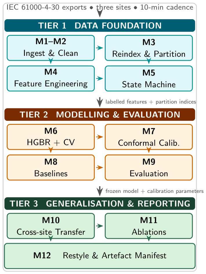
Figure 2.
Primary-site spectral characterisation. (a) Per-phase individual voltage harmonic distortion by order 2 to 11, with interquartile-range error bars; phase A is quietest while phases B and C show elevated triplen and upper-order content. (b) Neutral-conductor THD over the 77-day record (mean 33.7%, max 44.9%), confirming triplen dominance consistent with switched-mode supply loading. (c) Phase-B UTHD distribution with watch (, orange) and exceedance (, dark red) thresholds marked.
Figure 2.
Primary-site spectral characterisation. (a) Per-phase individual voltage harmonic distortion by order 2 to 11, with interquartile-range error bars; phase A is quietest while phases B and C show elevated triplen and upper-order content. (b) Neutral-conductor THD over the 77-day record (mean 33.7%, max 44.9%), confirming triplen dominance consistent with switched-mode supply loading. (c) Phase-B UTHD distribution with watch (, orange) and exceedance (, dark red) thresholds marked.
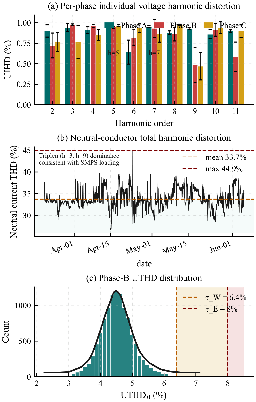
Figure 3.
Test MAE (pp) on phase-B UTHD versus forecast horizon for all seven methods, with block-bootstrap 95% confidence bands on the HGBR variants. The two proposed models form the lowest error band at every horizon. Ridge regression degrades sharply above 60 min; ARIMA holds near 0.71 pp throughout. The annotation confirms versus all baselines at each horizon.
Figure 3.
Test MAE (pp) on phase-B UTHD versus forecast horizon for all seven methods, with block-bootstrap 95% confidence bands on the HGBR variants. The two proposed models form the lowest error band at every horizon. Ridge regression degrades sharply above 60 min; ARIMA holds near 0.71 pp throughout. The annotation confirms versus all baselines at each horizon.
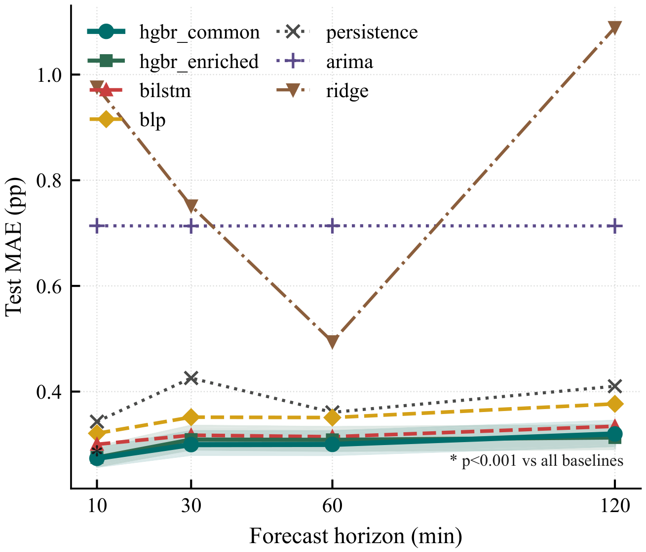
Figure 4.
Phase-B UTHD forecast with 90% and 95% adaptive conformal prediction intervals over the test window (28 May to 5 June). The dashed line marks . The annotation near 5 June identifies a region of elevated nonconformity that triggers adaptive interval widening.
Figure 4.
Phase-B UTHD forecast with 90% and 95% adaptive conformal prediction intervals over the test window (28 May to 5 June). The dashed line marks . The annotation near 5 June identifies a region of elevated nonconformity that triggers adaptive interval widening.
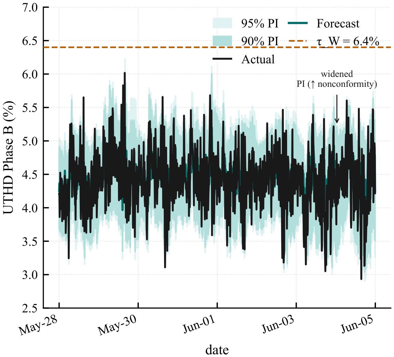
Figure 5.
Coverage-width trade-off analysis. (a) Empirical coverage (solid, left axis) and mean PI width (dashed, right axis) versus mixing parameter at for (teal) and (red); the vertical dashed line marks the locked . (b) M-sensitivity frontier in coverage-width space for ; the star marks the locked operating point (, ). Coverage reaches 89.9% at and 90.8% at .
Figure 5.
Coverage-width trade-off analysis. (a) Empirical coverage (solid, left axis) and mean PI width (dashed, right axis) versus mixing parameter at for (teal) and (red); the vertical dashed line marks the locked . (b) M-sensitivity frontier in coverage-width space for ; the star marks the locked operating point (, ). Coverage reaches 89.9% at and 90.8% at .
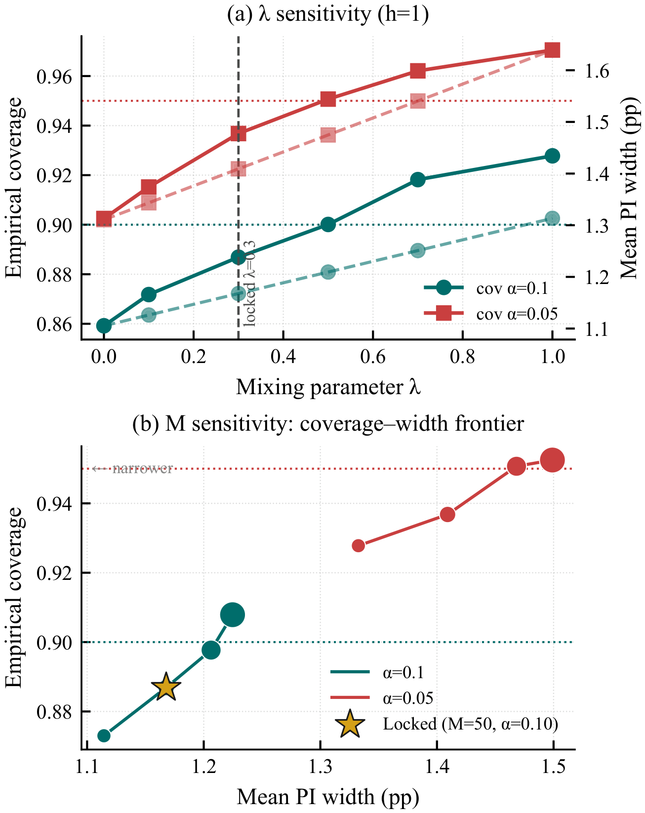
Figure 6.
Phase-B UTHD under frozen-model cross-site transfer with 90% conformal bands; the point predictor is frozen and the conformal layer is recalibrated on a small labelled target-site calibration subset. (a) Córdoba (source domain): MAE pp, exceedance . (b) Site A (frozen transfer): MAE pp, exceedance ; forecast held above actual. (c) Site B (frozen transfer): MAE pp, exceedance ; forecast tracks actual more closely. Dashed line marks .
Figure 6.
Phase-B UTHD under frozen-model cross-site transfer with 90% conformal bands; the point predictor is frozen and the conformal layer is recalibrated on a small labelled target-site calibration subset. (a) Córdoba (source domain): MAE pp, exceedance . (b) Site A (frozen transfer): MAE pp, exceedance ; forecast held above actual. (c) Site B (frozen transfer): MAE pp, exceedance ; forecast tracks actual more closely. Dashed line marks .
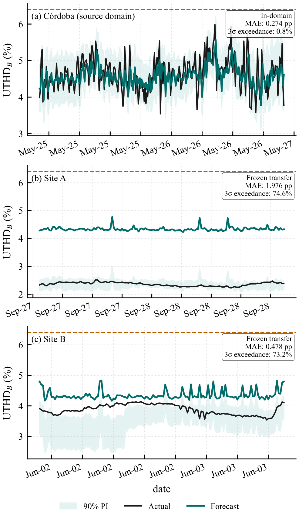
Figure 7.
Ablation studies on phase-B UTHD. (a) Test MAE (pp) versus forecast horizon for the four feature subsets; all curves lie within pp at . (b) FAR versus watch threshold for all four horizons; the dashed line marks the locked .
Figure 7.
Ablation studies on phase-B UTHD. (a) Test MAE (pp) versus forecast horizon for the four feature subsets; all curves lie within pp at . (b) FAR versus watch threshold for all four horizons; the dashed line marks the locked .
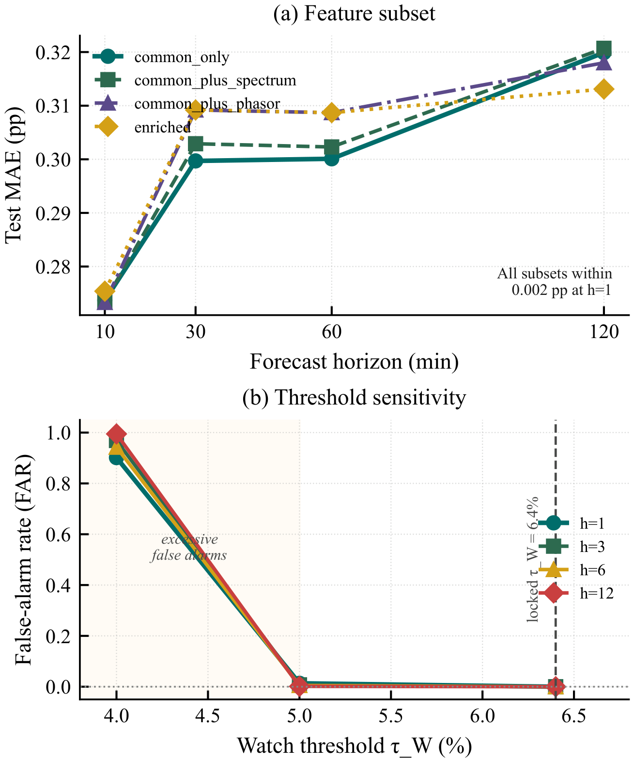

Table 1.
Dataset partitioning and compliance composition across the three sites.
| Site | Total | Train | Calib. | Test | Normal % |
|---|---|---|---|---|---|
| Córdoba (primary) | 11,088 | 7,762 | 1,663 | 1,663 | 99.90 |
| Site A (external) | 1,001 | 701 | 150 | 150 | 100.00 |
| Site B (external) | 965 | 676 | 145 | 144 | 100.00 |
Table 2.
Watch-threshold sweep on phase B at the primary site.
| Raw Normal | Raw Watch | Conf. Normal | Conf. Watch | |
|---|---|---|---|---|
| 1,518 | 9,570 | 634 | 10,454 | |
| 9,349 | 1,739 | 10,093 | 995 | |
| 11,077 | 11 | 11,085 | 3 |
Table 3.
Per-phase point accuracy of the proposed model with block-bootstrap 95% CIs. All MAE and RMSE values are in pp.
Table 3.
Per-phase point accuracy of the proposed model with block-bootstrap 95% CIs. All MAE and RMSE values are in pp.
| Target | Horizon | MAE [95% CI] | RMSE | sMAPE |
|---|---|---|---|---|
| UTHD-A | 10 min | 0.056 [0.052, 0.059] | 0.072 | 2.56% |
| UTHD-A | 30 min | 0.079 [0.071, 0.083] | 0.102 | 3.60% |
| UTHD-A | 60 min | 0.104 [0.092, 0.111] | 0.133 | 4.77% |
| UTHD-A | 120 min | 0.128 [0.110, 0.139] | 0.163 | 5.86% |
| UTHD-B | 10 min | 0.274 [0.259, 0.296] | 0.357 | 6.20% |
| UTHD-B | 30 min | 0.309 [0.291, 0.335] | 0.397 | 6.95% |
| UTHD-B | 60 min | 0.309 [0.288, 0.333] | 0.400 | 6.94% |
| UTHD-B | 120 min | 0.313 [0.292, 0.336] | 0.410 | 7.03% |
| UTHD-C | 10 min | 0.274 [0.259, 0.295] | 0.354 | 6.29% |
| UTHD-C | 30 min | 0.308 [0.290, 0.334] | 0.394 | 7.06% |
| UTHD-C | 60 min | 0.298 [0.279, 0.321] | 0.385 | 6.83% |
| UTHD-C | 120 min | 0.311 [0.290, 0.333] | 0.403 | 7.10% |
Table 4.
Diebold-Mariano tests on phase-B UTHD at the 10-min horizon. Reference: HGBR enriched.
| Challenger | DM Statistic | p-Value | Proposed Wins |
|---|---|---|---|
| Persistence | Yes | ||
| ARIMA | Yes | ||
| Ridge | Yes | ||
| Beta-LP | Yes | ||
| BiLSTM | Yes |
Table 5.
Conformal interval performance on the primary test set, phase B. Width values are in pp.
| Horizon | Cov. 90% | Width 90% | Cov. 95% | Width 95% |
|---|---|---|---|---|
| 10 min | 0.887 | 1.168 | 0.937 | 1.409 |
| 30 min | 0.893 | 1.264 | 0.941 | 1.547 |
| 60 min | 0.892 | 1.276 | 0.935 | 1.533 |
| 120 min | 0.894 | 1.325 | 0.939 | 1.601 |
Table 6.
Frozen-model cross-site transfer on phase-B UTHD. MAE values in pp.
| Site | 10 min | 30 min | 60 min | 120 min |
|---|---|---|---|---|
| Córdoba (in-domain) | 0.274 | 0.300 | 0.301 | 0.320 |
| Site A (transfer) | 1.977 | 2.353 | 2.014 | 2.100 |
| Site B (transfer) | 0.478 | 0.499 | 0.501 | 0.515 |
Table 7.
Covariate shift relative to the frozen source scaler.
| Site | Rows | Frac. | ||
|---|---|---|---|---|
| Córdoba | 11,088 | 0.12 | 0.07 | 0.001 |
| Site A | 1,001 | 75.25 | 39.20 | 0.556 |
| Site B | 965 | 25.42 | 10.64 | 0.580 |
Disclaimer/Publisher’s Note: The statements, opinions and data contained in all publications are solely those of the individual author(s) and contributor(s) and not of MDPI and/or the editor(s). MDPI and/or the editor(s) disclaim responsibility for any injury to people or property resulting from any ideas, methods, instructions or products referred to in the content. |
© 2026 by the authors. Licensee MDPI, Basel, Switzerland. This article is an open access article distributed under the terms and conditions of the Creative Commons Attribution (CC BY) license (http://creativecommons.org/licenses/by/4.0/).
Copyright: This open access article is published under a Creative Commons CC BY 4.0 license, which permit the free download, distribution, and reuse, provided that the author and preprint are cited in any reuse.