

Submitted:
08 September 2026
Posted:
09 September 2026
You are already at the latest version
Abstract
The vertical wind profile within the Atmospheric Boundary Layer (ABL) is a critical variable 2
for a wide range of applications, including wind energy, air traffic and unmanned aerial 3
system (UAS) management, pollutant dispersion, and urban air mobility. However, its 4
accurate characterization typically requires expensive vertical-profiling LiDAR instruments, 5
which limits the number of locations that can be simultaneously monitored. Building upon 6
previous work in which machine-learning algorithms were trained on LiDAR data from the 7
University of León (Spain) to reconstruct full ABL wind profiles from a single near-surface 8
measurement, this study replaces the traditional data-driven neural network approach with 9
Physics-Informed Neural Networks (PINNs), embedding a physical constraint directly into 10
the loss function as evaluated by automatic differentiation, and tests two such constraints 11
under architectural control: the Ekman boundary-layer momentum balance, closed with a 12
Monin-Obukhov eddy viscosity, and a shear-constrained formulation based on a power-law 13
profile with an inferred exponent. With dense supervision at the target heights, neither 14
constraint improves on an architecture-matched network without a physical term (RMSE 15
1.35-1.36 m/s, direction MAE 20.1-20.4◦ across all three, Kruskal-Wallis p = 0.0125), and 16
in a vertical-extrapolation protocol, training with gates up to 111 m, selecting models 17
by their skill at 140 m, and testing blind on 170-300 m, the Ekman constraint shows 18
no advantage over its own architectural control, but the shear-constrained model does, 19
reaching 1.80 ± 0.01 m/s speed RMSE and 27.0◦ ± 0.3◦ direction MAE against 2.66 ± 0.10 20
m/s and 34.2◦ ± 1.8◦ for the Ekman-constrained arm and 2.61 ± 0.12 m/s and 33.9◦ ± 21
2.0◦ for the physics-free arm, which are statistically indistinguishable from one another; 22
the shear-constrained gain is confirmed against its own architectural control (2.64 ± 0.08 23
m/s, 33.0◦ ± 1.8◦, matching the physics-free arm), ruling out the additional output as 24
the explanation, and converts an erratic extrapolator into a stable one. The benefit of 25
embedding physics into the loss is therefore specific to the extrapolation regime and to the 26
formulation tested, not a generic property of physics-informed learning. By eliminating the 27
need for continuous LiDAR operation after the training phase, the proposed methodology 28
aims to enable cost-effective monitoring of multiple locations with a single instrument.
Keywords:
physics-informed neural networks (PINNs)
; atmospheric boundary layer
; wind profile estimation
; LiDAR
; physics-informed learning
; power-law wind profile
; Ekman layer
; Monin-Obukhov similarity theory
1. Introduction
The vertical wind profile within the Atmospheric Boundary Layer (ABL) is a fundamental atmospheric variable whose accurate characterization is critical for a wide range of engineering and environmental applications. In the wind energy sector, knowledge of the vertical wind shear across the rotor swept area directly conditions annual energy production estimates and fatigue load calculations [1,2]. In air traffic management, wind profile information is essential for fuel-efficient climb and descent procedures, as well as for the safe operation of Unmanned Aerial Systems (UAS) in low-altitude corridors [3]. Additional applications include pollutant dispersion modeling, urban microclimate analysis, numerical weather prediction initialization, and the planning of advanced air mobility operations.
Traditionally, the gold-standard instrument for measuring the complete ABL wind profile up to several hundred metres above ground level is the Doppler wind Light Detection And Ranging (LiDAR) system. Coherent Doppler wind LiDAR provides profiles with high vertical and temporal resolution, directly measuring wind speed and direction at multiple altitude bins simultaneously [4,5]. However, the high acquisition and operational costs of LiDAR instruments impose a significant practical constraint: continuous monitoring of multiple geographical sites with dedicated instrumentation is economically unfeasible for most organizations, thereby limiting the spatial density of observations. Low-cost anemometric stations, in contrast, are widely deployed but provide only near-surface point measurements, leaving the upper portion of the ABL unobserved.
This observational gap has motivated the development of model-based methods to reconstruct full ABL wind profiles from limited near-surface data. Classical approaches rely on semi-empirical laws, such as the logarithmic wind profile valid in the surface layer and the power-law profile applicable throughout the entire ABL, to extrapolate measured wind speeds to higher altitudes [1,2]. While computationally straightforward, these analytical models assume idealized atmospheric conditions (neutral stratification, horizontal homogeneity) and struggle to capture the variability introduced by thermal stratification, complex terrain, and non-stationary atmospheric conditions. Mesoscale numerical weather prediction models such as the Weather Research and Forecasting (WRF) model can provide three-dimensional wind fields at kilometre-scale resolution, but their spatial and temporal resolution remain insufficient for many local applications, and significant deviations from observed profiles are common in stable or convective regimes.
The emergence of machine learning (ML) has opened a new avenue for ABL wind profile estimation. Data-driven approaches are capable of learning complex, nonlinear mappings between near-surface observations and the full wind profile directly from historical datasets, without relying on explicit physical parameterizations. García-Gutiérrez et al. [3] introduced one of the earliest methodologies of this kind, training a multilayer perceptron (MLP) on LiDAR data collected at the University of León (Spain) to reconstruct the ABL wind profile from a single near-ground measurement, using the three most recent 10-min measurements of the wind components (six input nodes); the method demonstrated substantially better performance than classical analytical profiles. A subsequent study by the same research group [6] extended the approach by incorporating predictions from the WRF mesoscale model as additional inputs, further improving reconstruction accuracy and enabling the exploration of the temporal evolution of the wind profile. More recently, Gu et al. [7] demonstrated a neural-field approach that fuses data from Doppler LiDAR and wind profiler radar to reconstruct a continuous, high-resolution urban wind field, reporting a mean absolute error of 0.55 m/s for wind speed in a real-world deployment over Guangzhou, China. In parallel, Bi et al. [8] applied backpropagation neural networks to replicate operational horizontal line-of-sight wind retrievals from the Aeolus spaceborne Doppler wind LiDAR, demonstrating the suitability of data-driven emulators across altitudes from 0 to 20 km. On the signal-processing side, Song et al. [4] showed that convolutional neural network architectures (U-Net) can effectively denoise coherent Doppler LiDAR spectrograms in low signal-to-noise conditions, further extending the usable detection range within the ABL.
Despite the promising results obtained with purely data-driven architectures, these approaches share a common limitation: they are agnostic to the physical laws governing boundary-layer dynamics. As a consequence, trained networks may produce wind profiles that violate known physical constraints, such as the logarithmic surface-layer scaling or Monin-Obukhov similarity theory, particularly when they are evaluated in atmospheric conditions that are underrepresented in the training dataset. Furthermore, purely data-driven models tend to overfit when the available labeled data are scarce, a situation that frequently arises in site-specific LiDAR campaigns of limited duration.
Physics-Informed Neural Networks (PINNs), introduced by Raissi et al. [9], offer a principled solution to these shortcomings by embedding governing differential equations or known physical laws directly into the loss function of the neural network. During training, the network is penalized not only for deviations from the data (data loss) but also for violations of the underlying physics (physics loss), evaluated at collocation points by automatic differentiation of the network output, yielding solutions that are simultaneously consistent with observations and with the problem’s governing equations. This hybrid approach has demonstrated superior generalization with limited data, improved robustness to noise, and physically consistent extrapolation in domains ranging from fluid dynamics [10] to heat transfer and structural mechanics. In wind science, PINNs have so far been applied mainly to spatial flow-field reconstruction, embedding the Navier-Stokes or Reynolds-averaged Navier-Stokes equations to recover turbulent ABL flow fields from sparse LiDAR data and validating against large-eddy simulations; these approaches, however, require dense multi-dimensional spatial information to constrain the full momentum equations and target three-dimensional field assimilation rather than the reconstruction of a one-dimensional vertical profile from a single ground point. In the atmospheric sciences more broadly, physics-informed machine learning has been increasingly adopted: for example, Tao et al. [11] highlighted the physics-informed deep learning framework as a promising direction for combining physical constraints with neural-network retrievals in satellite remote sensing, while boundary-layer profile applications remain comparatively unexplored.
The present study builds upon the previous data-driven work carried out at the University of León [3,6] and proposes two key advances. First, the training dataset is substantially enlarged by incorporating additional years of LiDAR observations, improving the statistical representativeness of the model across a broader range of atmospheric stability conditions and seasonal variability. Second, the conventional data-driven framework is replaced by physics-informed formulations, and two structurally different physical constraints are evaluated under identical architecture so that their contribution can be separated from that of the network itself. The first is the boundary-layer momentum balance appropriate to a one-dimensional vertical profile: the Ekman equations, closed with a height- and stability-dependent turbulent viscosity from Monin-Obukhov Similarity Theory (MOST). In its neutral surface-layer limit it recovers the logarithmic wind profile used as a baseline in the earlier studies; aloft it reproduces the Ekman spiral, that is, the simultaneous increase of wind speed and clockwise rotation (veering) of wind direction with height; and through the MOST closure it accounts for the stability dependence of vertical mixing. It is posed on the horizontal wind components (u, v) rather than on the speed modulus, so the network reconstructs wind direction as well as speed, which is the directional structure that the regime-clustering analysis of this dataset (Section 2.1.1) identifies as a defining feature of the nocturnal stable boundary layer at the site. The second is a parameterized shear constraint based on a power-law profile whose exponent is inferred per sample, imposed on the speed modulus alone and requiring only first derivatives of the network output. Comparing the two, against one another and against an architecture-matched network with no physical constraint, is what allows the contribution of the embedded physics to be assessed rather than assumed. The methodology is designed to eliminate the need for continuous LiDAR operation after the initial training phase, enabling cost-effective monitoring of multiple locations with a single instrument and significantly reducing overall deployment costs.
The remainder of this paper is organised as follows. Section 2 describes the LiDAR dataset, the data preprocessing procedure, the mathematical formulation of the physical constraints embedded in the loss function, and the PINN architectures. Section 3 presents the validation results, comparing three architecture-matched arms (an Ekman-constrained, a shear-constrained and a physics-free model) against one another and against classical analytical and tree-based baselines. Section 4 discusses the findings, and Section 5 summarizes the main conclusions and outlines directions for future research.
2. Materials and Methods
This section describes the observational dataset and the processing steps used to construct consistent input-target pairs for training and evaluation. It then introduces the governing equations, turbulence closure and shear constraint used to impose physical consistency in the learning problems, and details the neural-network architectures, loss formulations and training procedures adopted for the physics-informed models.
2.1. Data
The input dataset consists of vertically resolved Doppler LiDAR measurements of horizontal wind speed and direction, together with surface meteorological observations recorded at 10-min intervals. For each averaging period t, the LiDAR provides horizontal wind speed and wind direction at a set of fixed heights (), while a nearby surface meteorological station records near-surface wind speed , wind direction , air temperature , pressure , and relative humidity . The measurements were collected using a ZephIR300 continuous-wave profiling LiDAR (Campbell Scientific, Inc., Logan, UT, USA) installed in a suburban area on the University of León campus (León, Spain). The dataset used for model training spans 46 non-contiguous months between March 2021 and May 2026, comprising 190,033 ten-minute-averaged wind profiles. The instrument was configured to provide wind measurements at twelve heights between 20 and 300 m above ground level (AGL); a co-located surface meteorological station provides an additional near-surface reference at 2 m AGL (Section 2.3.2), giving thirteen vertical levels in total. The site is characterized by an aerodynamic roughness length of approximately 1.91 m, corresponding to Davenport terrain classifications representative of mixed low- and high-rise suburban environments.
Four distinct counts of "samples" appear throughout this study, and are used consistently as follows. Profiles refers to the 190,033 raw ten-minute LiDAR scans described above. Sequences refers to the 180,977 overlapping look-back windows retained after requiring finite ground-level features at every step and at least six valid altitude gates (Section 2.3.1); these are the units of the training, validation and test partitions (126,683 / 27,147 / 27,147, a 70/15/15 stratified split). Entries refers to individual (sequence, height) pairs with a genuine measurement, used when reporting per-sample statistical tests (e.g. 335,333 valid entries in the in-distribution test set, Section 3.3).
The ZephIR300 is capable of measuring wind speed and direction at heights ranging from 10 to 300 m, with a configurable set of user-defined height levels (twelve were configured for this deployment), a sampling frequency of 50 Hz, and a wind speed measurement range between 1 and 70 m s−1. The reported wind speed accuracy is 0.1 m s−1, while the wind direction accuracy is better than . Independent validation studies have reported a mean bias of approximately 0.1 m s−1 for horizontal wind speed measurements and about for wind direction measurements [12]. Consequently, rather than presenting these specifications in tabular form, the main LiDAR characteristics can be summarized as follows: measurement range of 10–300 m, twelve configured measurement heights, 50 Hz sampling rate, wind speed operating range of 1–70 m s−1, wind speed accuracy of 0.1 m s−1, and wind direction accuracy better than .
All data are stored using arrays for LiDAR profiles, altitudes and surface variables. Prior to model training, a basic quality-control step is performed on the LiDAR wind-speed profiles: for each time step t, the number of valid (non-missing) heights is counted, and profiles with fewer than a user-defined minimum number of valid levels (6, in the present study) are discarded. For the remaining samples, any missing values in the vertical profiles are handled as described in Section 2.3.1 .
2.1.1. Profile-Based Clustering with K-Means
To obtain a compact representation of typical vertical structures of the wind field (and, as motivated in the Introduction, to expose the directional regimes that the physical constraint must reproduce) an unsupervised clustering of the LiDAR profiles is performed using the K-Means algorithm. For each valid profile at time t, a feature vector is constructed concatenating the wind speed and the sine and cosine of the wind direction at all heights, i.e. . This choice avoids discontinuities associated with the circular nature of the wind direction. These variables fully describe the horizontal wind vector at each height (magnitude and direction), with the sine/cosine encoding avoiding the discontinuity; no additional features are used so that the clustering reflects the wind structure alone.
Before clustering, missing values in are imputed using a median-based imputer applied component-wise over the full training set, and the resulting features are standardized to zero mean and unit variance. K-Means clustering with clusters is then applied to the standardized vectors, using 20 different random initializations and a fixed random seed to ensure reproducibility. Only profiles with at least 6 valid heights are used to fit the clustering model. The resulting cluster labels c(t) ∈ {0, 1, 2} are subsequently assigned to all valid time steps.
The clustering analysis from the wind LiDAR profiler at the University of León successfully isolates three distinct atmospheric regimes, showing strong physical consensus between the K-Means and Agglomerative algorithms despite a structural label swap between their second and third clusters (Figure 1). Cluster 0 (C0) represents a classic Nocturnal Stable Boundary Layer (SBL) that dominates nighttime and early morning hours, particularly during the spring and summer (Figure 2). Driven by radiative cooling at the surface, this regime features low-to-moderate wind speeds (1.5 to 4.5 m/s) and significant directional shear, or veering. The wind vector rotates clockwise with height from a cool, localized northeastern katabatic drainage flow (~70°) near the surface, channeled from the adjacent Cantabrian Mountains into the basin, up toward a regional southeasterly synoptic flow (~140°) at 300 m, a behavior governed by frictional decoupling and the development of an Ekman spiral. This regime is the primary physical motivation for posing the Ekman model constraint on the wind components rather than on the speed modulus.
The second physical regime, designated as C1 in K-Means and C2 in Agglomerative clustering, captures a highly energetic, well-mixed daytime Convective Boundary Layer (CBL). This regime exhibits the highest recorded wind velocities in the dataset, accelerating from 3.5 m/s near the ground to nearly 10 m/s at 300 m, while maintaining a nearly constant westerly direction (~265°) across the entire vertical profile. The complete absence of directional shear is a direct consequence of intense solar heating during summer afternoons (15:00 to 20:00); the resulting turbulent convective plumes thoroughly homogenize vertical atmospheric momentum, effectively dragging high-velocity synoptic Atlantic winds down through the boundary layer across the Iberian plateau.
The third regime, identified as C2 in K-Means and C1 in Agglomerative clustering, represents a moderate daytime flow (3.5 to 5.5 m/s) driven by regional thermal forcing, operating primarily during spring and summer middays (12:00 to 18:00). Similar to the westerly regime, the wind direction profile here is vertically uniform due to active solar convection, maintaining a steady southern to southeasterly heading (~175°). This cluster physically tracks the diurnal development of the Iberian Thermal Low (Baja Térmica), a seasonal low-pressure system generated by the intense solar heating of the peninsula’s interior landmass. This thermal depression acts as a synoptic vacuum, drawing warmer air masses from the south northward toward León, where it is captured as a distinct, shear-free vertical column.
The power spectral density (PSD) of horizontal wind speed at three measurement heights (20 m, 111 m, and 270 m) is shown in Figure 3 as a function of frequency (left panel) and as the variance-preserving spectrum f·S(f) versus period (center panel), computed with Welch’s method on 10-min averaged LiDAR records (t = 600 s). The absolute energy level increases substantially with altitude across the entire resolved frequency band (), reflecting the suppression of wind variability near the surface by friction and the growth of mean wind speed with height within the atmospheric boundary layer. At the two upper levels (111 m and 270 m) the spectral slope in the high-frequency range closely follows the Kolmogorov inertial-subrange scaling, consistent with locally isotropic, well-developed turbulence detached from the direct influence of the surface. At 20 m, however, the slope is noticeably shallower than , indicating an excess of high-frequency variance relative to the inertial-subrange prediction; this is a well-known signature of the surface layer, where mechanical shear and proximity to the ground continuously inject energy at small scales and the turbulence departs from local isotropy [12].
The variance-preserving form f·S(f) (center panel) isolates the dominant energy-containing scales as explicit peaks. A pronounced peak near the 12-day timescale is evident at all three heights and intensifies markedly with altitude, pointing to synoptic-scale pressure systems as the primary driver of wind variability at this site. The progressive suppression of this synoptic peak towards the surface is consistent with increased frictional decoupling of the near-ground flow from the large-scale forcing. No distinct diurnal (24 h) or semi-diurnal (12 h) peak is discernible, suggesting that thermally driven local circulations are either weak at this location or their variance falls below the noise floor of the Welch estimator for the chosen segment length. The cumulative energy fraction (right panel) confirms that the bulk of the wind variance is concentrated at low frequencies for all heights: at 270 m and 111 m approximately 60% of the total energy lies below (periods longer than ~3 h), whereas the 20-m level accumulates energy more slowly towards low frequencies, reflecting its relatively larger contribution from high-frequency turbulent fluctuations. The dominance of low-frequency, synoptic-scale variability and the multi-hour autocorrelation it implies motivate the use of a recurrent (LSTM) encoder over the surface history, rather than an instantaneous mapping, in the model described below.
2.2. Preprocessing
Prior to model training, the raw surface and LiDAR time series are transformed into synchronised, quality-controlled inputs and targets suitable for sequence learning. Surface measurements are encoded into an 8-dimensional feature vector per 10-min interval, combining wind speed, wind direction represented by and , thermodynamic and humidity variables, and short-term tendencies via first differences of wind speed and temperature; missing values are propagated as NaNs and handled consistently during subsequent filtering.
Training samples are then constructed by sliding a fixed-length temporal window of steps over the ground-feature series to form input sequences , which are retained only when the corresponding LiDAR profile contains at least 6 valid levels, the regime label is defined, and all entries in are finite. The model uses two targets: a regression target given by the vertical wind profile expressed in Cartesian components , and a classification target given by the regime label. Physically implausible wind speeds are flagged as missing, remaining gaps are imputed using altitude-wise medians, and the profile targets are standardized by altitude to improve numerical conditioning, with the scaling parameters stored for inverse transformation of predictions.
2.3. Methods
This subsection describes the learning framework used to map short histories of ground-based observations to instantaneous vertical wind profiles and their associated flow regimes. First the multi-task Bi-LSTM architecture that encodes the input sequences into a shared latent representation and branches into regression and classification heads is introduced, then the training procedure and loss formulation, and finally two physical constraints tested within this framework: the Ekman boundary-layer balance (Section 2.3.2) and the parameterized shear constraint (Section 2.3.3).
2.3.1. Multi-Task Bi-LSTM Architecture
A multi-task recurrent encoder-decoder is used to map a short history of ground-based inputs (with ) to (i) the instantaneous LiDAR wind profile and (ii) its associated regime label. The model is implemented in TensorFlow/Keras [13] and consists of a two-layer bidirectional LSTM (Bi-LSTM) encoder followed by a shared dense layer that produces a compact latent context vector. From this shared representation, the network branches into two heads: a regression head that reconstructs the profile and a classification head that predicts the regime. Profile reconstruction is performed with a height-conditioned decoder in which the context vector is concatenated with the (normalized) query height and passed through fully connected layers to output the standardized wind components at that height; representing the profile as a continuous function of height enables vertical derivatives by automatic differentiation, which is required by the physics-informed extension (Section 2.3.2). The shear-constrained and physics-free arms reuse this architecture, adding only an output for the shear exponent where relevant (Table 1).
Training uses stratified splits (70% training, 15% validation, 15% test) to preserve the cluster distribution. Ground-feature sequences are standardized using statistics from the training set and the same transform is applied to validation and test data. The shared encoder is optimized in a multi-task setting using Adam [14] to minimize a weighted sum of the profile mean-squared error and the sparse categorical cross-entropy for regime classification, with early stopping and learning-rate reduction on plateau; each physics-informed arm follows the corresponding procedure within its own custom training loop (Section 2.3.2, Section 2.3.3). Performance is reported on the held-out test set using wind-speed RMSE (overall and per-height) and MAE for the regression task, circular (wrap-aware) direction error obtained from the predicted components, and overall regime-classification accuracy; correlation and distributional metrics (Pearson correlation and Jensen-Shannon divergence) are additionally computed for wind-resource relevance.
The architecture and training configuration are selected via Bayesian optimization with Keras Tuner [15,16] by minimizing a validation objective. The search spans LSTM widths, decoder and context dimensions, learning rate, batch size, the look-back window , and the weights and scheduling of the physics and boundary-condition terms; to accommodate the custom training loop, the tuner is integrated via Keras Tuner’s public API for custom trial execution, using Bayesian optimization. The configuration selected for the Ekman-constrained arm is then reused, unchanged, for the shear-constrained and physics-free arms, so that the three differ only in their physics terms. The search space and the selected configurations are summarized in Table 1.
2.3.2. First Extension to a Physics-Informed Neural Network (Ekman Balance)
The multi-task Bi-LSTM architecture of Section 2.3.1 is extended to a Physics-Informed Neural Network by (i) reformulating the regression target as the two horizontal wind components (u, v) at each height, from which speed and direction are recovered, and (ii) augmenting the architecture with a physics head and replacing standard supervised training with a custom training loop that evaluates the boundary-layer momentum residual by automatic differentiation.
In the stationary, horizontally homogeneous boundary layer, the mean horizontal momentum balance is given by the Ekman system:
where (u, v) are the wind components, the geostrophic wind, the Coriolis parameter at the site latitude N (giving f ), and (z) the turbulent (eddy) viscosity. Rather than assuming a constant , which would impose a neutral, idealized spiral, the system is closed with the Monin-Obukhov form:
with the von Kármán constant, d the zero-plane displacement height, fixed to throughout this study, since the vegetation and building height in the immediate vicinity of the LiDAR unit do not justify a significant displacement, notwithstanding the mixed low- and high-rise character of the wider site (Section 2.3.2), the friction velocity, L the Obukhov length, and the Businger-Dyer stability function [17] ( for stable with ; for unstable with ). In the neutral surface-layer limit (, small z), Eq. (2) gives and the system reduces to the logarithmic profile; aloft, Eq. (1) governs the Ekman spiral, reproducing the directional veering documented for the nocturnal stable regime in Section 2.1.1 [18]. The closure thus embeds the logarithmic, Ekman, and stability physics within a single constraint.
From the shared latent vector, a small dense head outputs four physically interpretable, sample-specific latent variables: the friction velocity > 0 (softplus activation), the inverse Obukhov length (linear activation, free sign, encoding stability), and the geostrophic components . These are inferred jointly with the profile, making the model an inverse-problem PINN. The profile decoder takes the latent vector concatenated with a normalized height z and returns ; because z enters explicitly and continuously, the derivatives , and the flux divergence are obtained by nested automatic differentiation at arbitrary collocation heights, including heights between and above the measured levels.
The network simultaneously minimizes a profile regression loss, a regime classification loss, and the Ekman residual:
where is the MSE between predicted and observed (u, v) at the measured heights (scale-normalized); is the sparse categorical cross-entropy of the regime head (); anchors the surface condition (u, v) → 0 at z0 + d; and is the mean squared Ekman residual:
with and , evaluated at collocation heights drawn freshly each step over the profile range, and residuals normalized by the scale to balance the loss terms. The vertical derivatives in the residual are not computed by finite differences over the LiDAR gates but by automatic differentiation of the continuous decoder, evaluated at a set of collocation heights sampled at each training step. At every such height, u, and are obtained at the same point, so the residual is defined pointwise and there is no dimensional mismatch with the data term. The weight (default ) controls the strength of the physics constraint; it is increased on a curriculum (data-dominated first, physics progressively hardened), as PINNs train poorly when the physics term dominates prematurely [19], and gradients are clipped by global norm for stability. Early stopping is monitored on the validation data loss rather than the total loss, ensuring that the physics term does not prematurely halt training before the profile fit has converged. The preprocessing pipeline, dataset splitting, and evaluation metrics are shared across all three arms (Section 2.3.1).
2.3.3. Second Extension to a Physics-Informed Neural Network (Parameterized Shear)
The Ekman balance is one of several physical descriptions that can be imposed on a vertical wind profile, and its structure, a second-order balance coupling the two horizontal components through Coriolis, is only one way in which a physical constraint can be posed. Whether the benefit of embedding physics into the loss depends on this specific choice, or holds more generally, is tested with a second, structurally different constraint: a power-law shear relation. Unlike the Ekman balance, which follows from the momentum equation under stated simplifying assumptions (stationarity, horizontal homogeneity), the power-law profile is semi-empirical: it can be derived from mixing-length arguments under a power-law eddy-viscosity profile, but it is more commonly justified by its long record of fit to observed surface-layer profiles across a wide range of terrain and stability conditions. It is included precisely because it rests on a different kind of physical justification than the Ekman balance, so that agreement or disagreement between the two constraints is informative about whether the benefit of physics-informed learning here is tied to the mechanistic detail of the Ekman equations or to the presence of any physically motivated shape constraint on the profile.
The power law is the standard engineering description of the surface-layer wind profile,
where is the shear exponent, an empirical function of atmospheric stability and surface roughness, typically reported in the range 0.1-0.4 over land. Differentiating Eq. (5) with respect to height removes the dependence on any particular reference level and yields a form that can be imposed pointwise on the decoder,
with the wind-speed modulus. The corresponding residual is
evaluated at the same collocation heights and normalized by the same velocity scale as the Ekman residual, so that the two are comparable in magnitude.
The exponent is not a free curve-fitting parameter but is understood to depend on the same physical factors that MOST parameterizes through and L: it increases with atmospheric stability (larger under stable stratification, where vertical mixing is suppressed and shear is concentrated near the surface) and with surface roughness, and decreases under unstable, well-mixed conditions, where turbulence homogenizes momentum through depth and the profile flattens. In this sense the two constraints tested encode overlapping physical information through different functional forms: the Ekman balance parameterizes the turbulent viscosity directly, while the power law parameterizes the resulting profile shape. Because enters the constraint algebraically rather than through a second-order balance, it does not require an eddy-viscosity closure of its own, and consequently carries no explicit stability parameter analogous to .
Two differences from the Ekman formulation are relevant to the interpretation of the results. First, is inferred per sample by an additional output of the physics head, rather than fixed as in the classical power-law baseline of Section 3.3; it is bounded to by a scaled sigmoid, covering the physically reported range with margin. Second, and unlike the Ekman balance, the constraint is imposed on the speed modulus alone and says nothing about wind direction, so any directional improvement it produces is indirect. Only first derivatives of the network output are required, making this residual computationally cheaper than the Ekman one, which needs the divergence of the turbulent flux.
The residual admits a degenerate solution analogous to the one documented for the Ekman closure (Section 2.3.2): a profile with negligible shear () trivially satisfies when as well, regardless of whether a flat profile is the physically correct description at that sample. Unlike the Ekman case, this degeneracy is not suppressed by an explicit bound analogous to the clamp; the only constraint on is the sigmoid range itself. In practice, of test samples saturate the lower bound (; Section 3.4), a non-negligible fraction, while saturation at the upper bound is rare (). Whether this reflects genuinely well-mixed conditions or an unconstrained escape route at the lower end of the exponent’s range cannot be resolved from the aggregate error metrics alone and is left for further investigation, for instance by anchoring to an independent bulk estimate, as is optionally anchored in the Ekman formulation (Section 2.3.2).
2.4. Vertical-Extrapolation Protocol
The comparisons of Section 3.1, Section 3.2, Section 3.3, Section 3.4, Section 3.5 and Section 3.6 evaluate the models at heights where abundant training data are available, a regime in which a physics prior can at best be neutral. To test the physics residual where it can, in principle, contribute information that the data cannot, the evaluation is recast as vertical extrapolation. The data loss is restricted to the LiDAR gates at z ≤ 111 m together with the surface anchor described below, the gate at 140 m is reserved as a height-band validation set, and the five gates between 170 and 300 m constitute a held-out test never used for training, early stopping, or hyperparameter selection. All model-selection decisions (the Bayesian search over architecture and loss weights, and the stopping epoch) are driven exclusively by the extrapolation error on the 140 m band, so that the amount of physics is itself selected by out-of-band skill rather than fixed a priori.
Three arms are compared, all sharing the architecture selected for the Ekman-constrained model (Table 1): the Ekman-constrained model, the shear-constrained model of Section 2.3.3, and a physics-free network in which neither physical term is active and the corresponding physics-head outputs receive no gradient. Holding architecture fixed across the three arms isolates the contribution of each physical constraint from that of the network itself. The physics weights (the Ekman residual weight and its warm-up, the friction-velocity anchor weight, and the shear residual weight) exist only in the arm to which they apply. As a classical reference, the logarithmic and power-law profiles are fitted by least squares on the same supervised gates and extrapolated upward; the random forest, being a fixed-grid regressor, cannot predict at unsupervised heights and is therefore excluded from the extrapolation comparison.
The Ekman formulation incorporates three components specific to the extrapolation setting; the shear-constrained formulation, imposed on the speed modulus alone with no eddy-viscosity closure, requires none of them beyond the shared surface anchor. First, the profile is anchored to the measured surface-station wind, from the AIRMAR ultrasonic anemometer at 2 m AGL [6], rather than to a no-slip condition at , which would contradict the non-zero measured surface wind; since (Section 2.3.2), this no-slip alternative would in any case coincide with m, well below the 2 m anemometer height, so the two anchor choices are not in physical conflict, only in whether the surface measurement itself is used. Second, the Monin-Obukhov stability argument in the eddy-viscosity closure is clamped to the empirical validity range of the similarity functions ( [18]). This constraint is necessary because the unconstrained residual admits a degenerate minimum whereby the inferred friction velocity is driven toward zero or is inflated, annihilating and reducing the Ekman balance to a pull of the profile toward an arbitrary per-sample constant . This mode is harmless where data supervise the profile but severely degrades the unsupervised heights, and an unclamped closure accordingly extrapolates worse than the physics-free arm, so the clamp is what allows the physical constraint to help rather than hurt above the observed column. Third, an optional regularizer anchoring the inferred friction velocity to the neutral bulk log-law estimate at the lowest supervised gate is included in the search space; the band-driven selection assigns it zero weight, indicating that the structural clamp alone suffices to keep the closure well conditioned.
For the shear-constrained arm, the constraint of Eq. (6) is evaluated at the same collocation heights as the Ekman residual, including those above the supervised range, so that continues to be inferred, and the profile shape continues to be constrained, at heights the model never observes labels for. The surface anchor is the same measured wind used by the Ekman arm; because the constraint acts on the speed modulus alone, only the anchor’s magnitude enters Eq. (5), and the reconstructed direction at every height is supplied by the network’s decoder rather than by the physical constraint, unlike in the Ekman formulation, where direction emerges from the coupled balance itself.
Comparisons on the held-out gates use only genuine (non-imputed) measurements and identical sample-retention criteria across all pipelines, so that every model is evaluated on the same set of test sequences. Of the 27,147 test sequences, 25,743 have a genuine LiDAR measurement at all five held-out gates simultaneously (300–170 m) and are used for the paired per-sample comparisons reported below; the remainder have a data gap at one or more of these gates. Statistical significance is assessed with per-sample paired Wilcoxon signed-rank tests on the common set of 25,743 test sequences. The data split is fixed across all runs, and training stochasticity is assessed with four seeds per arm.
3. Results
All results below use the common look-back window (three hours of surface history), identified as optimal for the shared architecture (Section 2.3.1). Section 3.1, Section 3.2, Section 3.3, Section 3.4, Section 3.5 and Section 3.6 evaluate on the standard in-distribution test set (all heights); the vertical-extrapolation protocol of Section 3.7 instead holds out the upper gates, as defined in Section 2.4. The paired statistical test and the per-altitude profiles use the identical stratified test partition for every model, so the comparison is strictly head-to-head, and reported errors are wind-speed errors in m/s unless stated otherwise.
3.1. Overall and Per-Altitude Error
Table 2 summarizes the aggregate test performance, compared on an equal footing: every model reconstructs the full wind vector (the random forest predicts the horizontal components at each height, from which speed and direction are recovered; the analytical laws, which have no rotation physics, are assigned the surface direction held constant with height). The shear-constrained arm has the lowest overall wind-speed error (RMSE 1.346 m/s), closely followed by the Ekman-constrained arm (1.351 m/s) and the physics-free arm (1.360 m/s); the three are statistically close (Section 3.2). The random forest (1.798 m/s) and the three analytical profiles (power-law 2.005, logarithmic 2.018, constant 2.968 m/s) trail clearly behind all three. On direction, the three architecture-matched arms (MAE 20.1-20.4°) are comparable, and are lower than the random forest (27.5°) and the analytical laws (35.1°). The three architecture-matched arms also attain the lowest Jensen-Shannon divergence from the measured speed distribution among all models (0.0044-0.0047, against 0.030 for the random forest and 0.032-0.21 for the analytical laws (Section 3.3)), and each physics-informed arm exposes an inferred latent variable that the classical and tree-based baselines do not provide: the friction velocity for the Ekman arm, and the shear exponent for the shear-constrained arm (Section 3.4).
The per-altitude structure of the error is shown in Figure 4. Wind-speed RMSE grows monotonically with height for every model, reflecting the increasing distance from the near-surface anchor. The three architecture-matched arms track one another closely at every height, from about 0.37 m/s at the surface to 2.12-2.16 m/s at 300 m; the classical laws and the random forest separate clearly above them, exceeding 2.8 m/s at the top of the profile (constant ≈ 4.1 m/s). Direction MAE follows the same pattern: the three arms rise together from about 10° at the surface to 27-29° at 300 m, while the random forest ranges more widely (2.5° at the surface to 37.6° at 300 m) and the three analytical laws, restricted to the no-veering surface direction, are exactly zero at the surface by construction and the highest aloft, identical to one another ( at 300 m).
3.2. Comparison Across Physical Constraints
The Ekman-constrained arm, the shear-constrained arm, and the physics-free arm share the architecture selected for the Ekman-constrained arm (Table 1), so the comparison isolates the effect of the physical constraint rather than mixing it with architectural differences. Table 2 summarizes the result: the three arms attain near-identical performance (RMSE 1.346-1.360 m/s, direction MAE 20.1-20.4°), all within one another’s seed-to-seed spread; a Kruskal-Wallis test across the three groups gives for RMSE, a difference that is statistically detectable but an order of magnitude smaller than the gap seen in vertical extrapolation (Section 3.7). A paired Wilcoxon test on a single representative seed pair (Ekman versus shear-constrained, in-distribution samples) confirms this: the Ekman arm is better in 50.2% of samples for speed MAE and 49.5% for direction error, indistinguishable from chance despite the large sample size making both differences formally significant ( and respectively). With dense supervision at the target heights, the choice of physical constraint, or its absence, has essentially no effect. Against the classical and tree-based baselines (Section 3.3), the Ekman-constrained arm reduces the per-altitude RMSE by 20-65% versus the constant profile and by 20-40% versus the logarithmic and power-law profiles across most of the column (Figure 5), and attains the lowest divergence from the observed speed distribution (Section 3.3) together with the interpretable friction velocity (Section 3.4) that neither the shear-constrained nor the physics-free arm currently exposes in the same way. Section 3.7 revisits this comparison in a vertical-extrapolation setting, where the picture changes.
3.3. Comparison with Analytical and ML Baselines
Figure 6a ranks the three architecture-matched arms by overall test RMSE, and Figure 6b-d compare the predicted and measured wind-speed distributions. The aggregate speed error of Table 2 is markedly lower for the three architecture-matched arms than for the random forest or any of the three analytical laws, confirmed by a paired Wilcoxon signed-rank test on per-sample speed MAE: the Ekman-constrained arm is more accurate than the random forest in 59.7% of samples (median 0.525 vs. 0.789 m/s), than the power-law and logarithmic profiles in 66.8-67.2% (median 0.572 vs. 1.03-1.05 m/s, restricted to the 308,186 entries where these profiles are defined; both are undefined at the surface gate), and than the constant profile in 75.7% (median 0.525 vs. 1.605 m/s), all at . The shear-constrained arm gives an indistinguishable picture (medians 0.529-0.577 m/s across the same four comparisons, 59.6-75.6% better), consistent with the near-equivalence of the two constrained arms established throughout this study. The classical laws are strongly penalized by the site’s extrapolation geometry: anchoring at the 2 m surface station over terrain whose Davenport roughness is z0 ≈ 1.9 m makes the single-anchor logarithmic and power-law profiles ill-conditioned, and the least-squares fit of the logarithmic profile drives its effective roughness down to z0 ≈ 0.05 m, far below the physical value, purely to compensate. The power-law exponent is fitted analogously by least squares on the training set rather than fixed to a literature value, giving the power-law baseline the same fair treatment. This effective (non-physical) roughness is itself evidence that a single-height extrapolation anchor is inadequate over this site, motivating the column-aware physical constraint adopted here. The Ekman-constrained arm attains a Jensen-Shannon divergence between predicted and measured speed distributions of 0.0047 (Table 2, Figure 6), matched by the shear-constrained arm (0.0047) and closely followed by the physics-free arm (0.0044); all three are far better than the random forest (0.0299), power-law (0.0323), logarithmic (0.0354) and constant (0.2060) models. This indicates that the three architecture-matched arms reproduce the statistical distribution of wind speed more faithfully than any classical or tree-based alternative, a property of direct relevance to wind-resource assessment, where the speed histogram, not the time-matched error, governs energy-yield estimates.
The same pattern holds for direction, with the same paired test: the Ekman-constrained arm is more accurate than the random forest in 59.7% of samples (median vs. ) and than all three analytical laws’ shared no-veering reference in 70.5% ( vs. ), all at ; the shear-constrained arm gives an indistinguishable picture ( median, 59.9-70.6% better across the same comparisons). The aggregate direction MAE of Table 2 shows the shear-constrained arm performing comparably to the Ekman-constrained arm overall ( against ), though, unlike the Ekman balance, the shear constraint acts on the speed modulus alone and does not itself impose any directional structure; the direction reconstructed by the shear-constrained arm is supplied entirely by the decoder rather than by the physical constraint (Section 2.4).
3.4. Inferred Physical Latent Variables
Beyond the wind field itself, the inverse-problem formulation yields sample-specific physical latent variables: the friction velocity for the Ekman-constrained arm, and the shear exponent for the shear-constrained arm (Section 2.3.1). This subsection examines first (Figure 7Figure 8), then (Figure 9Figure 10). Because no eddy-covariance or flux measurements are available at the site, cannot be validated directly against a measured reference; therefore it is assessed for physical plausibility and for consistency with the expected diurnal behavior. Figure 7 shows the distribution of the inferred over the test set: it is positively skewed with a median of 0.38 m/s and an interquartile spread consistent with values commonly reported over land surfaces, with the bulk of the mass between roughly 0.25 and 0.55 m/s and a tail extending to higher values under strong-wind conditions. These magnitudes are physically reasonable and are obtained without any direct supervision on , which enters training only through the Ekman+MOST residual.
The diurnal cycle of the inferred is shown in Figure 8. Averaging the test-set by local hour gives a daytime maximum and nocturnal minimum. The mean is lowest overnight (≈ 0.38-0.40 m/s between 00:00 and 07:00), rises through the morning, peaks in the early afternoon (≈ 0.80 m/s around 14:00), and decays towards the evening. This matches the expected surface-layer behavior (daytime solar heating drives convective mixing and a larger friction velocity, while the nocturnal surface layer is comparatively quiescent) and is recovered from surface inputs alone, without the time of day or any stability information as input. This diurnal cycle is a form of interpretability that the physics-free arm and the classical regressors do not provide; the shear-constrained arm offers an analogous latent variable, discussed below. This makes the friction velocity a second usable output of the reconstruction rather than an internal variable: from a single surface station the model returns both the vertical wind profile and a surface-layer scaling parameter that neither the physics-free arm nor the analytical laws provide, and that is required as an input by dispersion and load models. The other latent variable of the closure, the inverse Obukhov length 1/L, is not analyzed here: although required by the eddy-viscosity closure, its inferred sign does not match the stable/unstable partition expected from the diurnal cycle, indicating that it acts as an internal degree of freedom of the constraint rather than a directly interpretable stability diagnostic. Interpreting the inferred stability would require independent flux measurements and is left for future work.
The distribution and diurnal cycle of the inferred shear exponent are shown in Figure 9Figure 10. Its median (0.10) and mean (0.17) fall within the range typically reported for surface-layer wind profiles (0.1-0.4); of samples saturate the lower bound (Figure 9), predicting an essentially flat profile, a fraction large enough to merit the caution already noted in Section 2.3.3. Averaged by local hour, is lowest in the early afternoon ( at 13:00) and highest overnight ( at 00:00), the mirror image of the diurnal cycle found for : convective daytime mixing (high ) homogenizes momentum through depth and flattens the profile (low ), while the quiescent, poorly-mixed nocturnal stable layer (low ) concentrates shear near the surface (high ). This inverse relationship is recovered from surface inputs alone, with no explicit coupling imposed between the two constraints, and offers an internal physical consistency check between the two arms.
3.5. Distribution of the Error in Time and by Regime
To understand where the model succeeds and where it struggles, the per-sample test error is broken down by time of day, season and atmospheric regime, exploiting the timestamps and the K-Means regime labels retained for each test sample. Three consistent and physically coherent patterns emerge. First, the speed error is higher at night (RMSE 1.040 m/s) than during the day (0.962 m/s; day defined as 07:00-19:00 local), even though the daytime convective boundary layer carries stronger winds; the nocturnal stable layer, with its shallow structure and directional shear, is intrinsically harder to reconstruct from a surface anchor. This pattern, and its seasonal counterpart (error lowest in summer, highest in winter, tracking the seasonal prevalence of stable, weakly-forced conditions), hold consistently across all three architecture-matched arms (Figure 11). Resolved by regime (Figure 12), the nocturnal stable boundary layer (C0) is the hardest case for all three, while the two convective regimes are comparable to one another; the regime the clustering analysis of Section 2.1.1 identifies as the most structured is, consistently, the one hardest to reconstruct.
To illustrate how the models behave over time rather than in aggregate, Figure 13, Figure 14 and Figure 15 show measured and predicted time series at a reference height of 100 m over the longest continuous test window of each regime. In the convective regimes (C1, C2), where the profile is well mixed, all three architecture-matched arms track the measured speed closely. In the nocturnal stable regime (C0), all three follow the observed veering, unlike the analytical laws, which are held at the fixed surface direction throughout. These windows are representative examples, not a quantitative measure; the aggregate errors are those of Table 2 and Figure 12.
3.6. Sensitivity to the Training-Set Size
A practical question for single-instrument deployment is how much training data the method requires. To address it, the fixed architecture is retrained on progressively smaller subsets of the training pool, holding the validation and test partitions fixed so that every point is directly comparable, and varying only the volume and temporal sampling of the training data, for all three architecture-matched arms. Two sampling schemes are used: contiguous blocks of the first K months (K = 1, 2, 3, 6, 9, 12) and a distributed scheme retaining the first W days of every month (W = 7, 14). The results (Figure 16) show a monotonic degradation as data are removed for all three arms alike, from a full-record RMSE of 1.35-1.36 m/s (about 127,000 training samples) to 1.89-1.91 m/s with twelve contiguous months and 2.48-2.63 m/s with a single month. Across the six contiguous-month sizes, no arm is consistently better than the others: the shear-constrained arm has the lowest RMSE at one, nine and twelve months, the physics-free arm at two and six, and the Ekman arm at three, with all three within 0.02-0.15 m/s of one another at every size. At a comparable data budget the distributed sampling is more efficient than a contiguous block for all three: retaining fourteen days per month (about 58,000 samples) yields 1.71-1.72 m/s, lower than any contiguous configuration short of the full record, because distributing the sampling across the calendar captures seasonal variability that a single contiguous block does not; this operational recommendation is independent of the physical constraint used. In operational terms, a LiDAR that revisits a site periodically through the year yields lower error per measurement-day than one deployed for a single contiguous campaign of equal length. Unlike vertical extrapolation, where the shear-constrained arm separates cleanly from the other two at every training size (Section 3.7), no physical constraint shows a reliable advantage in-distribution regardless of how much training data is available.
3.7. Physics-Informed Vertical Extrapolation
Table 3 summarizes the held-out test (170-300 m). With architecture held fixed across the three arms, the Ekman-constrained arm ( m/s speed RMSE, direction MAE, mean ± sd over four seeds) is statistically indistinguishable from the physics-free arm ( m/s, ), extending to the extrapolation regime the null result already established in-distribution (Section 3.2). The shear-constrained arm, by contrast, separates cleanly from both: m/s and , a gap of roughly m/s and with no overlap in either range across seeds. Per sample, it is more accurate than the Ekman arm in 65-71% of held-out cases and than the physics-free arm in 65-68%, with p below floating-point resolution in every seed pairing. On the supervised gates the three arms are indistinguishable (0.73-0.75 m/s), so the shear constraint costs nothing where data govern the fit and extrapolates markedly better where they do not.
The most robust difference across the three arms is not the mean gap but the spread. Across four training seeds the physics-free arm ranges from 2.44 to 2.70 m/s and the Ekman arm from 2.52 to 2.73 m/s in speed RMSE, both overlapping substantially; the shear-constrained arm ranges from 1.79 to 1.81 m/s, with no overlap with either. Its worst seed is better than the best seed of both other arms, so which shear-constrained model one obtains from a given initialization is essentially predetermined, unlike the other two arms. A related consequence follows in model selection: in the tuning of the physics-free arm, the selected configuration achieved a marginally better validation-band score than the Ekman arm (0.1771 vs. 0.1779 in the normalized selection objective) and nevertheless performed no better on the held-out gates. Data-driven selection at 140 m cannot see what happens at 300 m; a residual that constrains the whole column and separates cleanly from the alternatives, as the shear constraint does, makes model selection robust precisely where the model is meant to be used.
This gap is tested against its own architectural control. The shear-constrained arm adds one output to the physics head (); an identical architecture with , the same output present but unused, attains m/s and , matching the physics-free arm rather than the shear-constrained one (Mann-Whitney against the shear-constrained arm in both metrics, four seeds each, no overlap in either range). The gap is therefore attributable to the residual, not to the additional output.
Figure 17 shows the error profiles. Without physics, the direction error diverges with height at an accelerating rate, exceeding at 300 m in the worst seed; the Ekman-constrained arm reaches a similar range (48- across seeds), while the shear-constrained arm remains below in every seed, never exceeding the best case of either alternative. The comparison with the fitted log law is, in aggregate, favourable to the constraint. The log law attains 2.39 m/s over the held-out gates, better than both the Ekman-constrained (2.66 m/s) and the physics-free (2.61 m/s) arms, reflecting the benign error tails of its rigid two-parameter form; the shear-constrained arm (1.80 m/s) is the only one of the three to improve on it. That same rigidity is the log law’s limitation: it holds the surface direction constant with height and cannot represent veering by construction, giving a direction error (42.4°) well above all three architecture-matched arms.
Resolving the held-out error by regime, using the shear-constrained arm against the physics-free arm as the controlled comparison, shows the RMSE advantage is large and consistent in all three regimes: C0 (1.96 vs 3.10 m/s), C1 (1.78 vs 2.38 m/s) and C2 (1.68 vs 2.52 m/s), with markedly smaller seed-to-seed spread for the shear-constrained arm throughout (sd 0.01-0.04 m/s against 0.18-0.35 m/s for the other two arms). The directional gain is not concentrated in the nocturnal stable regime C0, where the Ekman veering is strongest yet the gain is smallest (: vs ), but grows through the convective regime C1 (: vs ) and is largest in C2 (: vs ). The Ekman arm’s regime-resolved error ( in C0, in C1, in C2) is statistically indistinguishable from the physics-free arm’s in every regime, consistent with the near-null in-distribution and extrapolation results already established for that formulation (Section 3.2).
Beyond pointwise error, the shape of the reconstructed profiles gives a more mixed picture (Figure 18). The shear-constrained arm is markedly closer to the measured profile on two of five statistics: the fraction of decreasing-speed segments (0.16 vs 0.60 for the physics-free arm; measured 0.29) and speed curvature (0.013 vs 0.123; measured 0.030). On the remaining three, however, the shear-constrained arm over-smooths relative to the measurement rather than matching it: its direction curvature (1.15) undershoots the measured value (6.09) by more than the physics-free arm overshoots it (9.49), and the same pattern holds for the mean and spread of total turning, where the physics-free arm’s point estimate happens to sit closer to the measurement despite a seed-to-seed spread so large (sd exceeding the mean itself in two cases) that this apparent proximity is not a reliable finding. The physics-free arm’s profiles are, in short, rougher than reality and unreliable across seeds; the shear-constrained arm’s are smoother than reality but consistent. Neither fully reproduces the measured column’s texture.
Taken together with Section 3.2 and Section 3.6, these results delineate the regime dependence, and the formulation dependence, of the physics contribution. With dense supervision at the target heights, neither constraint tested improves on the physics-free arm. In vertical extrapolation, the Ekman-MOST residual is similarly neutral relative to its own architectural control, whereas the shear-constrained residual substitutes for tens of meters of unobserved column, improves the typical error over the classical extrapolation laws, recovers the veering that they cannot represent, and converts an unreliable extrapolator into a stable one.
4. Discussion
With architecture held fixed, the Ekman-constrained arm, the shear-constrained arm and the physics-free arm attain near-identical in-distribution performance (Section 3.2; Figure 4 shows this holds at every height), and remain close to one another across the full range of training-set sizes (Section 3.6; Figure 16). With dense supervision at the target heights, no physical constraint tested reduces the speed error relative to the same architecture without one.
Two properties distinguish the Ekman-constrained arm from the classical and tree-based baselines, though not from the other two architecture-matched arms. First, on wind direction (including the veering of the nocturnal stable regime C0, Section 2.1.1) all three architecture-matched arms attain comparable error (MAE -) and are more accurate than the random forest and the analytical laws, which cannot represent veering and default to the surface direction. Second, the Ekman-constrained arm exposes an interpretable latent variable, the friction velocity , whose inferred diurnal cycle (Section 3.4) tracks the expected convective daytime maximum and nocturnal minimum, that the MLP and tree regressors of the prior studies [3,6] cannot provide; the shear-constrained arm exposes an analogous latent variable, the shear exponent (Figure 9Figure 10), whose median lies within the range reported for surface-layer profiles, though a fraction of samples saturate its lower bound. The companion stability parameter of the Ekman closure (the inverse Obukhov length) is inferred jointly but does not admit a clean physical interpretation here, and is left for dedicated analysis with independent flux data.
The comparison against the classical baselines is unambiguous both in aggregate and per sample (Table 2; Section 3.3): the three architecture-matched arms attain roughly half the median error of the logarithmic and power-law profiles, are more accurate than the random forest in 59.6-59.7% of samples, and the constant profile is not competitive, all at . The analytical laws are particularly disadvantaged by the extrapolation geometry of this dataset, where the only near-surface anchor is the 2 m station. Over terrain with a Davenport roughness near 1.9 m, the single-anchor logarithmic profile is mathematically ill-conditioned, and fitting its roughness by least squares yields an effective that has no physical meaning and exists only to rescale the profile. That a standard surface-layer law must abandon its own physical parameter to remain usable is, in itself, an argument for a column-aware physical constraint that does not hinge on a single extrapolation base; Section 3.7 shows this benefit is realised in practice by the shear-constrained formulation, though not by the Ekman balance tested here.
Several limitations should be stated plainly. The Ekman balance assumes stationarity and horizontal homogeneity, both idealizations in the suburban, orographically influenced terrain of León, where katabatic drainage from the Cantabrian Mountains breaks horizontal homogeneity in the nocturnal regime; the constraint is therefore best understood as a soft physical prior rather than an exact equation the data must obey. PINN training is known to be sensitive to the weighting of the physics loss, which is why a small target Ekman weight and a curriculum ramp are required for stable convergence. Finally, the present comparison is confined to a single site. With architecture held fixed, no physical constraint tested reduces the in-distribution speed error at this site, whether at full training-set size or at any reduced budget (Section 3.6). One setting in which a physical prior is expected to reduce error, vertical extrapolation beyond the supervised heights, is tested in Section 3.7 and reverses this picture for the shear-constrained arm, though not for the Ekman formulation. There, the shear-constrained arm is decisively and consistently better on the held-out gates (Section 3.7). This advantage is not attributable to the Ekman closure’s own conditioning safeguards, such as clamping to the validity range of the similarity functions to remove degenerate minima of the Ekman residual (Section 2.3.2): the Ekman-constrained arm, despite this safeguard, shows no advantage over its own architectural control in extrapolation. The shear-constrained arm’s own residual carries an analogous, less-constrained degeneracy at the lower bound of the inferred exponent (Section 2.3.3), yet still extrapolates markedly better, suggesting the benefit lies in the shape of the constraint itself rather than in how tightly its degenerate solutions are suppressed. Two limitations of that protocol should be kept in mind: the selection band comprises a single gate, so configurations that are indistinguishable at 140 m can differ above it (the physics itself is what makes selection robust to this) and the analysis remains confined to one site. Transfer to sites not seen during training remains the most important direction for future work, together with a validation of the inferred stability parameter against independent flux measurements (its diurnal behavior does not presently match the expected stable/unstable partition, as noted in Section 3.4).
5. Conclusions
This work proposes a physics-informed neural network for reconstructing the full ABL vertical wind profile, in both speed and direction, from a single near-surface measurement, and tests two physical constraints, embedded directly into the training loss via automatic differentiation, under architecture control. The Ekman formulation closes the boundary-layer momentum balance with a stability-dependent Monin-Obukhov eddy viscosity and recovers the classical logarithmic profile as its neutral surface-layer limit; the shear-constrained formulation imposes a power-law shear relation with a per-sample inferred exponent. With dense in-distribution supervision, the two constrained arms and a physics-free arm of identical architecture attain statistically indistinguishable performance (RMSE 1.346-1.360 m/s, direction MAE 20.1-20.4°; Kruskal-Wallis , an order of magnitude smaller effect than found in extrapolation), a result that holds across the full range of training-set sizes tested. In a vertical-extrapolation protocol, where supervision stops at 111 m and the 170-300 m gates are held out, the Ekman formulation shows no advantage over the physics-free arm under the same architectural control, but the shear-constrained arm does: m/s and direction MAE, against m/s and for the Ekman arm and m/s and for the physics-free arm, which are indistinguishable from one another; the shear-constrained gain is confirmed against its own architectural control (a matched arm with the exponent output present but unused, m/s, ). The benefit of a physical constraint is thus specific to both the regime (extrapolation, not interpolation) and the formulation (shear constraint, not the Ekman balance), and is not a generic property of embedding physics into the loss. Future work will test additional physical formulations, transfer to sites not seen during training, and validate the inferred latent variables (, , ) against independent flux measurements.
Author Contributions
Conceptualization, A.G.-G. and A.D.; methodology, L.S. and R.E.; software, R.E. and F.P.; validation, A.D. and F.P.; formal analysis, R.E.; data curation, F.P and L.S.; writing-original draft, R.E.; writing-review and editing, A.G.-G, A.D. and L.S; supervision, A.G.-G and A.D. All authors have read and agreed to the published version of the manuscript.
Funding
This work was partly financed by the MCIN/AEI/10.13039/501100011033 and the European Communitarian Fund “ERDF A way of making Europe” funds within the scope of the projects PID2020-120496RB-I00 and UNLE15-EE-2977.
Data Availability Statement
The code supporting the results of this study is openly available on GitHub at https://github.com/redevhub/lidarpinn and archived with a permanent DOI on Zenodo at https://doi.org/10.5281/zenodo.21897456. The LiDAR dataset supporting the results is archived on Zenodo at https://doi.org/10.5281/zenodo.21904496.
Conflicts of Interest
The authors declare no conflict of interest.
References
- Garratt, J.R. The Atmospheric Boundary Layer; Cambridge University Press: Cambridge, UK, 1994. [Google Scholar]
- Stull, R.B. An Introduction to Boundary Layer Meteorology; Kluwer Academic Publishers: Dordrecht, The Netherlands, 1988. [Google Scholar]
- García-Gutiérrez, A.; Domínguez, D.; López, D.; Gonzalo, J. Atmospheric boundary layer wind profile estimation using neural networks applied to lidar measurements. Sensors 2021, 21, 3659. [Google Scholar] [CrossRef]
- Song, Y.; Han, Y.; Su, Z.; Chen, C.; Sun, D.; Chen, T.; Xue, X. Denoising coherent Doppler lidar data based on a U-Net convolutional neural network. Appl. Opt. 2024, 63, 275–282. [Google Scholar] [CrossRef]
- Kliebisch, O.; Uittenbosch, H.; Thurn, J.; Mahnke, P. Coherent Doppler wind lidar with real-time wind processing and low signal-to-noise ratio reconstruction based on a convolutional neural network. Opt. Express 2022, 30, 5540–5552. [Google Scholar] [CrossRef]
- García-Gutiérrez, A.; López, D.; Domínguez, D.; Gonzalo, J. Atmospheric Boundary Layer Wind Profile Estimation Using Neural Networks, Mesoscale Models, and LiDAR Measurements. Sensors 2023, 23, 3715. [Google Scholar] [CrossRef]
- Gu, T.; Liang, Y.; Yan, Y.; Jiang, W.; Yue, H.; Hu, G.; Zhang, J. Towards high-fidelity urban wind profiles for the built environment: a neural field to fuse multi-source observational data in Guangzhou, China. Build. Environ. 2026, 288, 114009. [Google Scholar] [CrossRef]
- Bi, Q.; Lv, J.; He, P.; Zhang, L. Rapid Aeolus L2B HLOS Wind Retrieval via BP Neural Network. Sensors 2026, 26, 1379. [Google Scholar] [CrossRef]
- Raissi, M.; Perdikaris, P.; Karniadakis, G.E. Physics-informed neural networks: A deep learning framework for solving forward and inverse problems involving nonlinear partial differential equations. J. Comput. Phys. 2019, 378, 686–707. [Google Scholar] [CrossRef]
- Cai, S.; Mao, Z.; Wang, Z.; Yin, M.; Karniadakis, G.E. Physics-informed neural networks (PINNs) for fluid mechanics: a review. Acta Mech. Sin. 2021, 37, 1727–1738. [Google Scholar] [CrossRef]
- Tao, M.; Zhao, Q.; Wang, W.; Man, W.; Zhou, S.; Tang, Z.; Fan, M.; Chen, L. Review of Satellite-Borne Multi-Angle Polarimetric Remote Sensing of Aerosols. Acta Opt. Sin. 2026, 46, 0600004. [Google Scholar] [CrossRef]
- Kaimal, J.C.; Finnigan, J.J. Atmospheric Boundary Layer Flows: Their Structure and Measurement; Oxford University Press: Oxford, UK, 1994. [Google Scholar]
- Abadi, M.; Barham, P.; Chen, J.; Chen, Z.; Davis, A.; Dean, J.; Devin, M.; Ghemawat, S.; Irving, G.; Isard, M.; Kudlur, M.; Levenberg, J.; Monga, R.; Moore, S.; Murray, D.G.; Steiner, B.; Tucker, P.; Vasudevan, V.; Warden, P.; Wicke, M.; Yu, Y.; Zheng, X. TensorFlow: A system for large-scale machine learning. Proc. 12th USENIX OSDI, 2016; pp. 265–283. [Google Scholar]
- Kingma, D.P.; Ba, J. Adam: A Method for Stochastic Optimization. In Proceedings of the 3rd International Conference on Learning Representations (ICLR), San Diego, CA, USA, 2015. [Google Scholar] [CrossRef]
- O’Malley, T.; Bursztein, E.; Long, J.; Chollet, F.; Jin, H.; Invernizzi, L.; et al. Keras Tuner. Available online: https://github.com/keras-team/keras-tuner (accessed on 10 June 2026).
- Snoek, J.; Larochelle, H.; Adams, R. Practical Bayesian Optimization of Machine Learning Algorithms. Adv. Neural Inf. Process. Syst. 2012, Vol. 25, 2951–2959. Available online: https://proceedings.neurips.cc/paper/2012/hash/05311655a15b75fab86956663e1819cd-Abstract.html (accessed on 3 July 2026).
- Businger, J.A.; Wyngaard, J.C.; Izumi, Y.; Bradley, E.F. Flux-profile relationships in the atmospheric surface layer. J. Atmos. Sci. 1971, 28, 181–189. [Google Scholar] [CrossRef]
- Foken, T. 50 Years of the Monin-Obukhov Similarity Theory. Bound.-Layer. Meteorol. 2006, 119, 431–447. [Google Scholar] [CrossRef]
- Krishnapriyan, A.S.; Gholami, A.; Zhe, S.; Kirby, R.M.; Mahoney, M.W. Characterizing possible failure modes in physics-informed neural networks. Adv. Neural Inf. Process. Syst. 2021, Vol. 34, 26548–26560. Available online: https://proceedings.neurips.cc/paper/2021/hash/df438e5206f31600e6ae4af72f2725f1-Abstract.html (accessed on 25 July 2026).
Figure 1.
PCA projection of the standardized wind profiles coloured by cluster, for K-Means (left) and Agglomerative (right) clustering with K = 3. The two algorithms agree on the three-regime structure up to a label swap between the second and third clusters.
Figure 1.
PCA projection of the standardized wind profiles coloured by cluster, for K-Means (left) and Agglomerative (right) clustering with K = 3. The two algorithms agree on the three-regime structure up to a label swap between the second and third clusters.
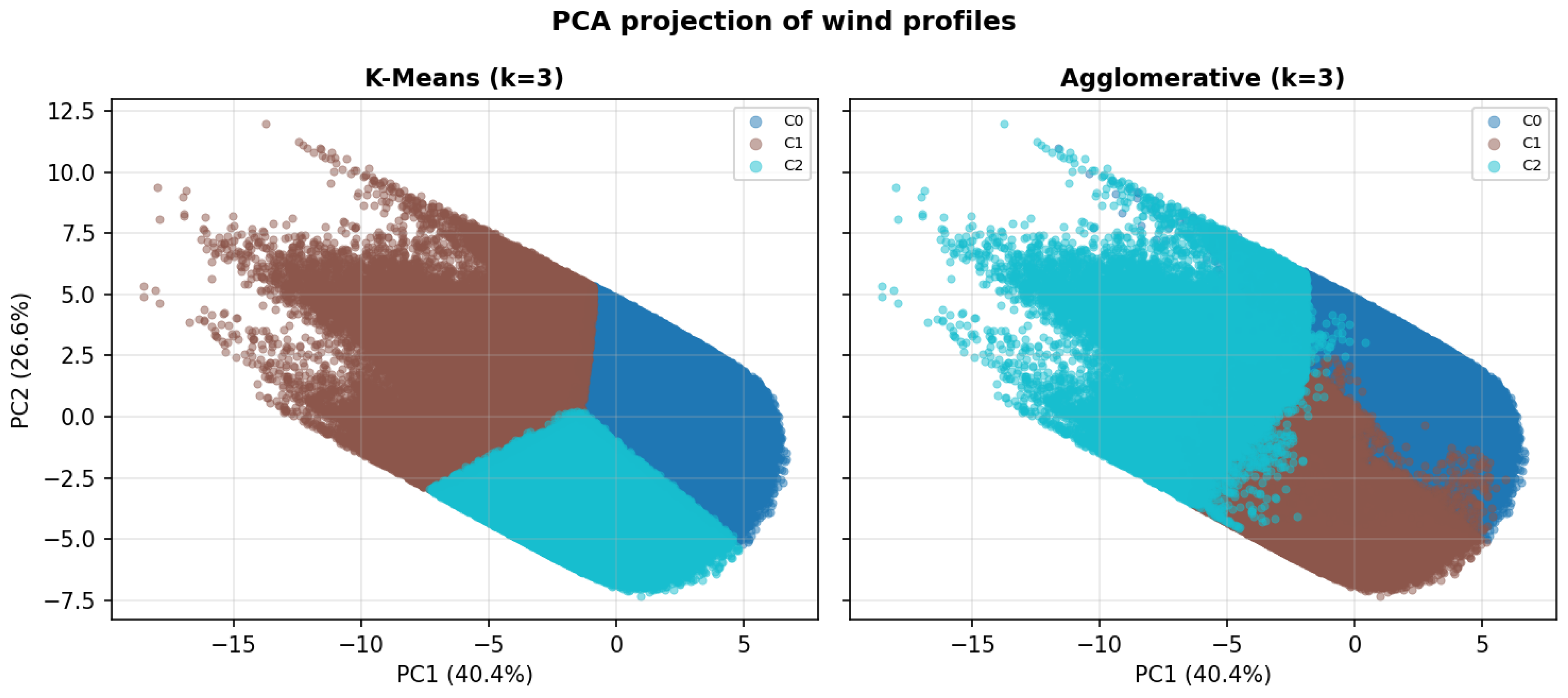
Figure 2.
Mean cluster profiles of wind speed (top) and wind direction (bottom) for K-Means (left) and Agglomerative (right) clustering. Shaded bands denote one standard deviation.
Figure 2.
Mean cluster profiles of wind speed (top) and wind direction (bottom) for K-Means (left) and Agglomerative (right) clustering. Shaded bands denote one standard deviation.
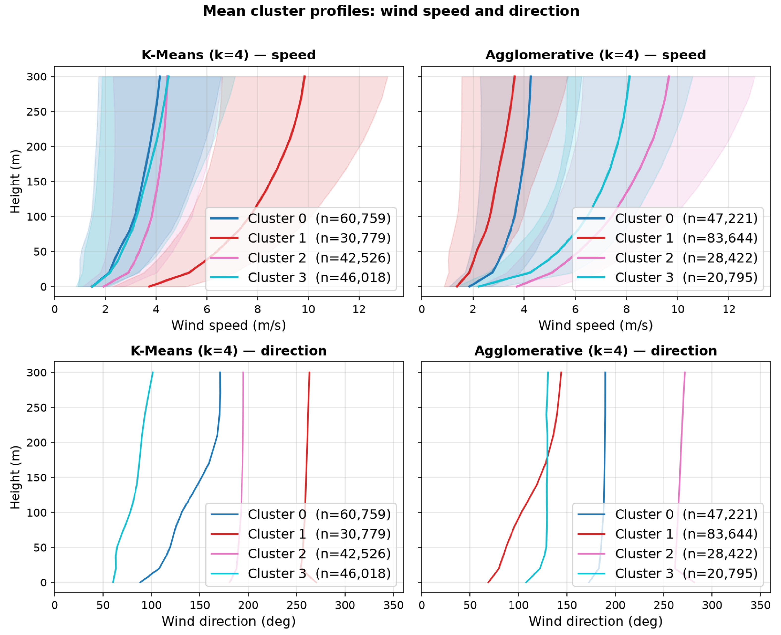
Figure 3.
Temporal wind-speed spectra at three measurement heights (20 m, 111 m, and 270 m), estimated with Welch’s method on 10-min averaged LiDAR records (t = 600 s). Left: power spectral density S(f) as a function of frequency (log-log scale); the dashed line indicates the Kolmogorov inertial-subrange reference slope. Center: variance-preserving spectrum f·S(f) as a function of period (log-linear scale), in which equal areas under the curve correspond to equal contributions to total variance; a dominant peak near the 12-day synoptic timescale intensifies with altitude. Right: normalized cumulative energy fraction as a function of frequency.
Figure 3.
Temporal wind-speed spectra at three measurement heights (20 m, 111 m, and 270 m), estimated with Welch’s method on 10-min averaged LiDAR records (t = 600 s). Left: power spectral density S(f) as a function of frequency (log-log scale); the dashed line indicates the Kolmogorov inertial-subrange reference slope. Center: variance-preserving spectrum f·S(f) as a function of period (log-linear scale), in which equal areas under the curve correspond to equal contributions to total variance; a dominant peak near the 12-day synoptic timescale intensifies with altitude. Right: normalized cumulative energy fraction as a function of frequency.
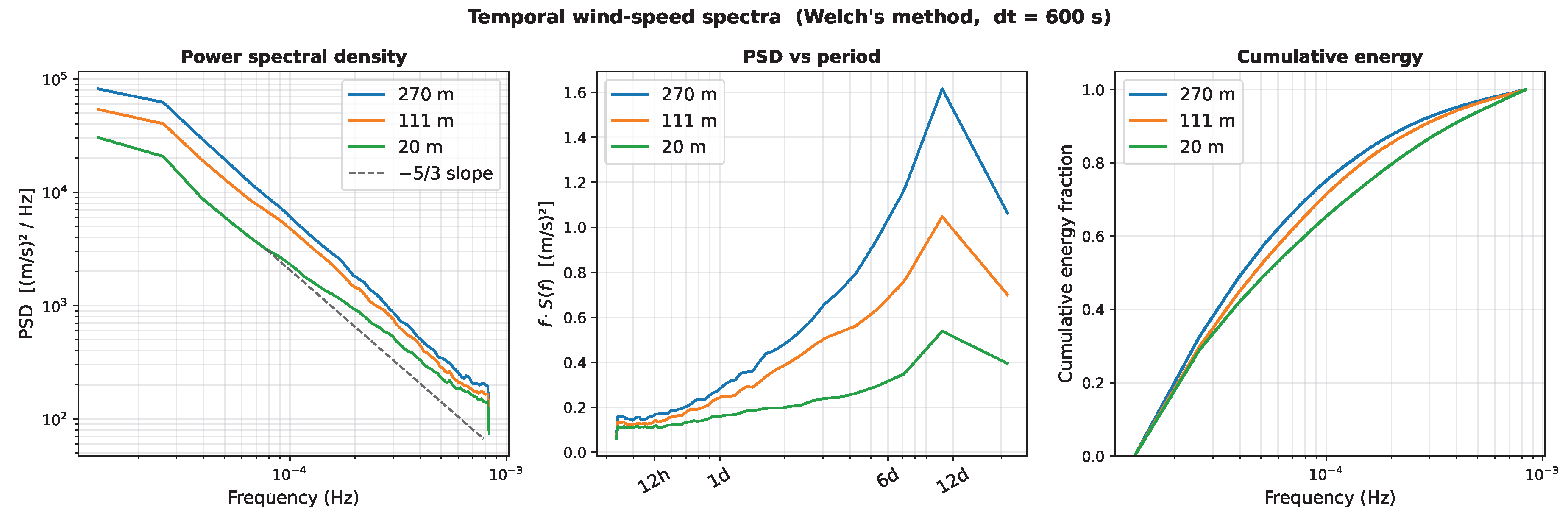
Figure 4.
Per-altitude wind-speed RMSE (a), MAE (b) and wind-direction MAE (c) on the in-distribution test set at . Solid lines with shaded envelopes: the three architecture-matched arms (Ekman-constrained, shear-constrained, physics-free), mean and min-max over four seeds. Dashed lines: the classical and tree-based baselines, single fixed models. The three architecture-matched arms are close to indistinguishable from one another throughout the column (Section 3.2).
Figure 4.
Per-altitude wind-speed RMSE (a), MAE (b) and wind-direction MAE (c) on the in-distribution test set at . Solid lines with shaded envelopes: the three architecture-matched arms (Ekman-constrained, shear-constrained, physics-free), mean and min-max over four seeds. Dashed lines: the classical and tree-based baselines, single fixed models. The three architecture-matched arms are close to indistinguishable from one another throughout the column (Section 3.2).
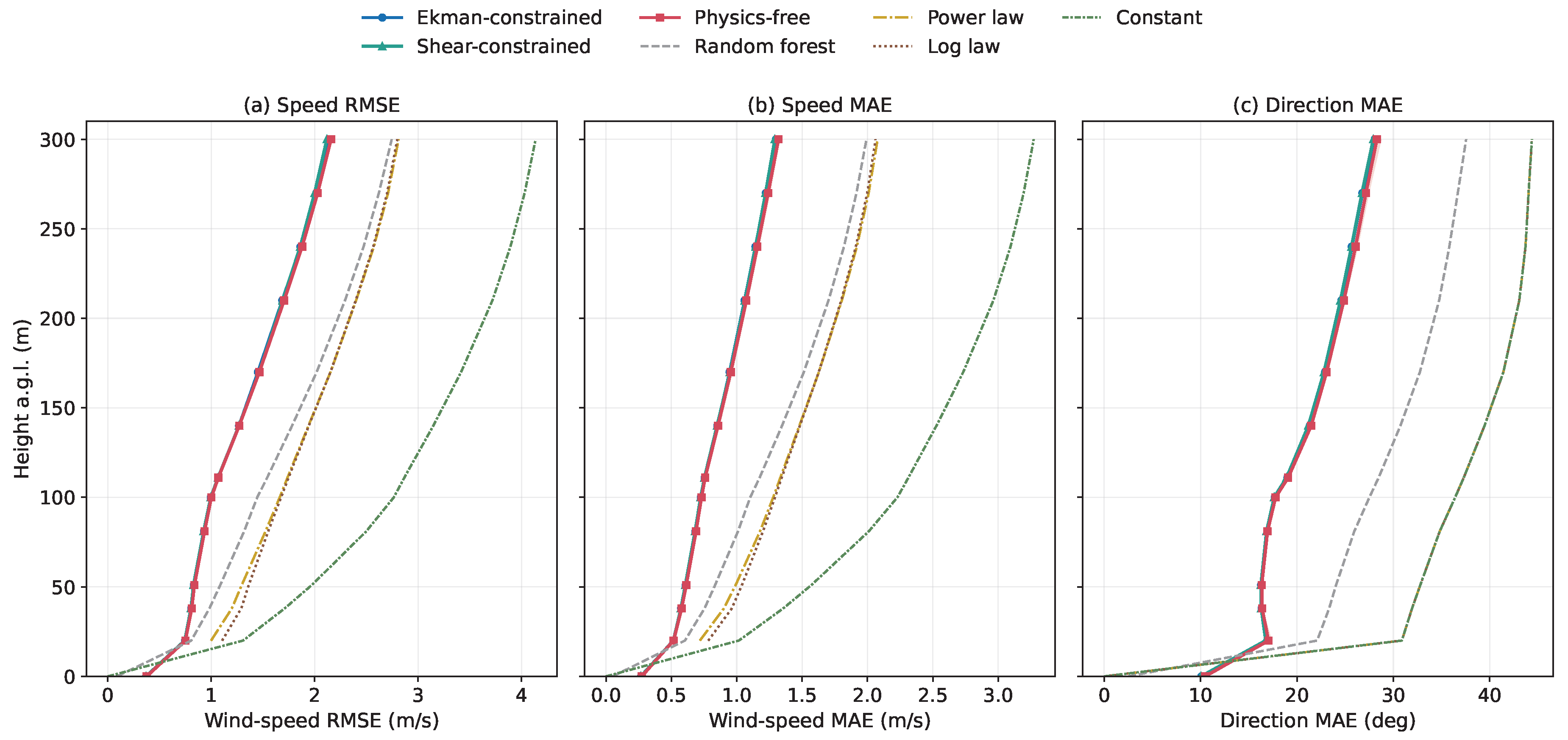
Figure 5.
Per-altitude RMSE reduction of the shear-constrained arm (the best-performing of the three architecture-matched arms, though not reliably distinguishable from the other two, Section 3.2) relative to each classical or tree-based baseline (positive = shear-constrained better). The logarithmic and power-law profiles are undefined at the surface (z = 0 m), the constant profile is anchored exactly to the surface measurement there, and random forest’s near-zero surface error makes the percentage reduction disproportionate; all are omitted at that height for clarity.
Figure 5.
Per-altitude RMSE reduction of the shear-constrained arm (the best-performing of the three architecture-matched arms, though not reliably distinguishable from the other two, Section 3.2) relative to each classical or tree-based baseline (positive = shear-constrained better). The logarithmic and power-law profiles are undefined at the surface (z = 0 m), the constant profile is anchored exactly to the surface measurement there, and random forest’s near-zero surface error makes the percentage reduction disproportionate; all are omitted at that height for clarity.
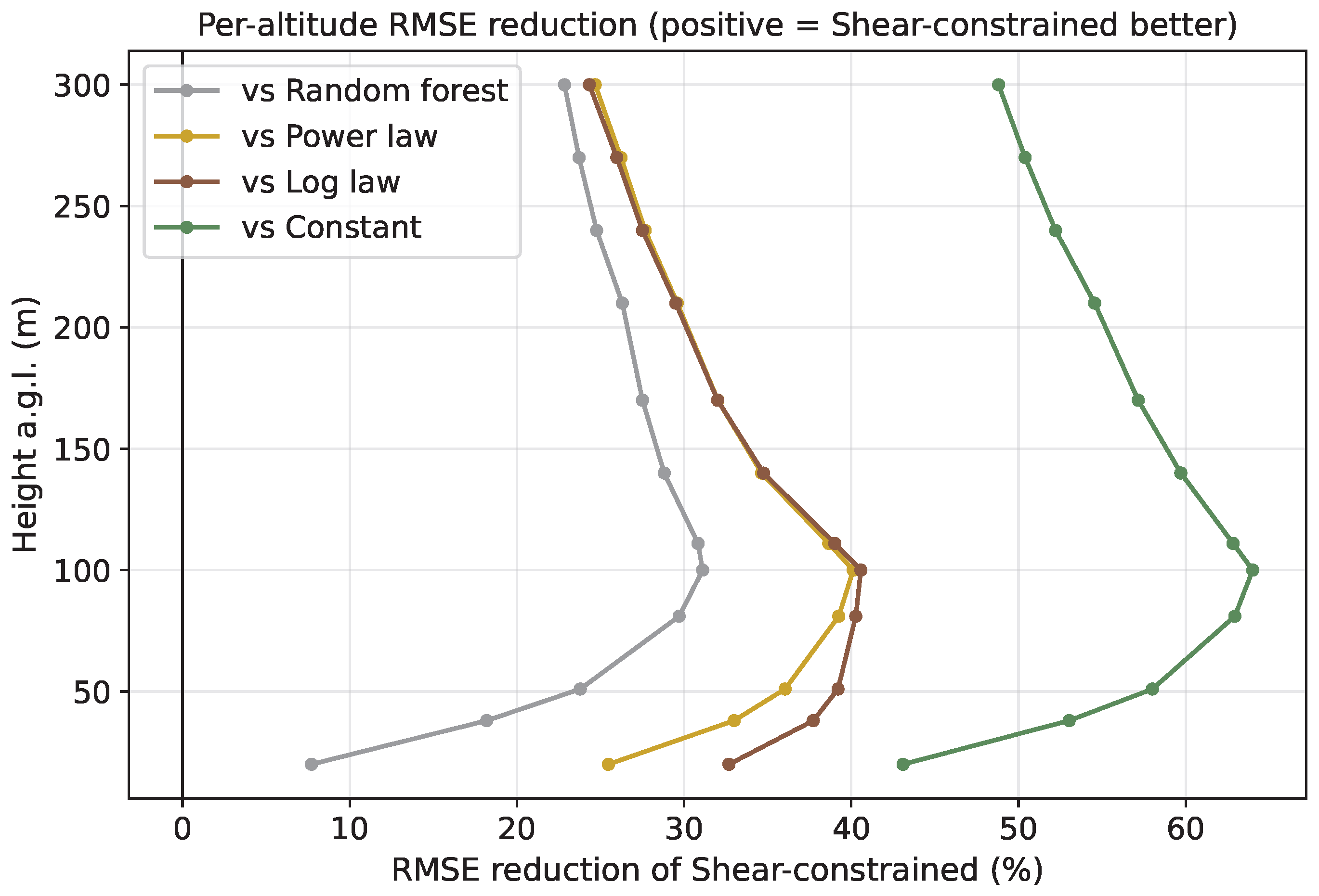
Figure 6.
(a) Overall in-distribution speed RMSE for the three architecture-matched arms, mean over four seeds, error bars one standard deviation. (b-d) Measured (grey) versus predicted (coloured) wind-speed probability densities for each arm, pooled over all four seeds, with the Jensen-Shannon divergence (JS). The classical and tree-based baselines are reported in Table 2 but not repeated here, since the histogram panels are already dense with three series.
Figure 6.
(a) Overall in-distribution speed RMSE for the three architecture-matched arms, mean over four seeds, error bars one standard deviation. (b-d) Measured (grey) versus predicted (coloured) wind-speed probability densities for each arm, pooled over all four seeds, with the Jensen-Shannon divergence (JS). The classical and tree-based baselines are reported in Table 2 but not repeated here, since the histogram panels are already dense with three series.
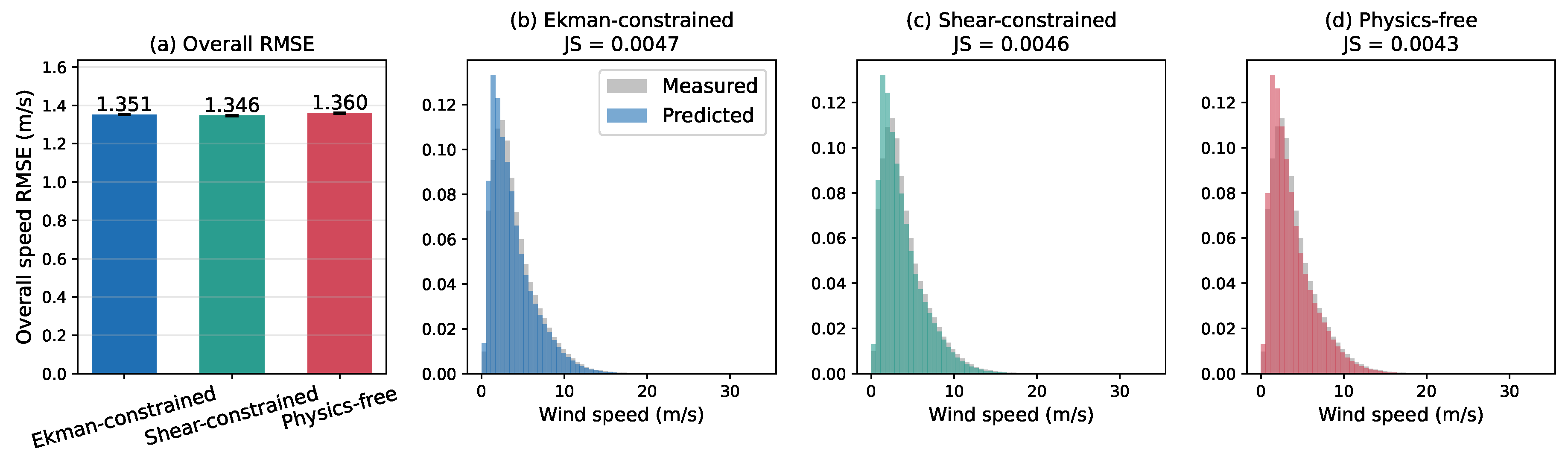
Figure 7.
Distribution of the friction velocity inferred by the physics head over the test set (median 0.38 m/s, dashed line). The magnitudes are physically plausible for a land surface and are obtained without direct supervision on .
Figure 7.
Distribution of the friction velocity inferred by the physics head over the test set (median 0.38 m/s, dashed line). The magnitudes are physically plausible for a land surface and are obtained without direct supervision on .
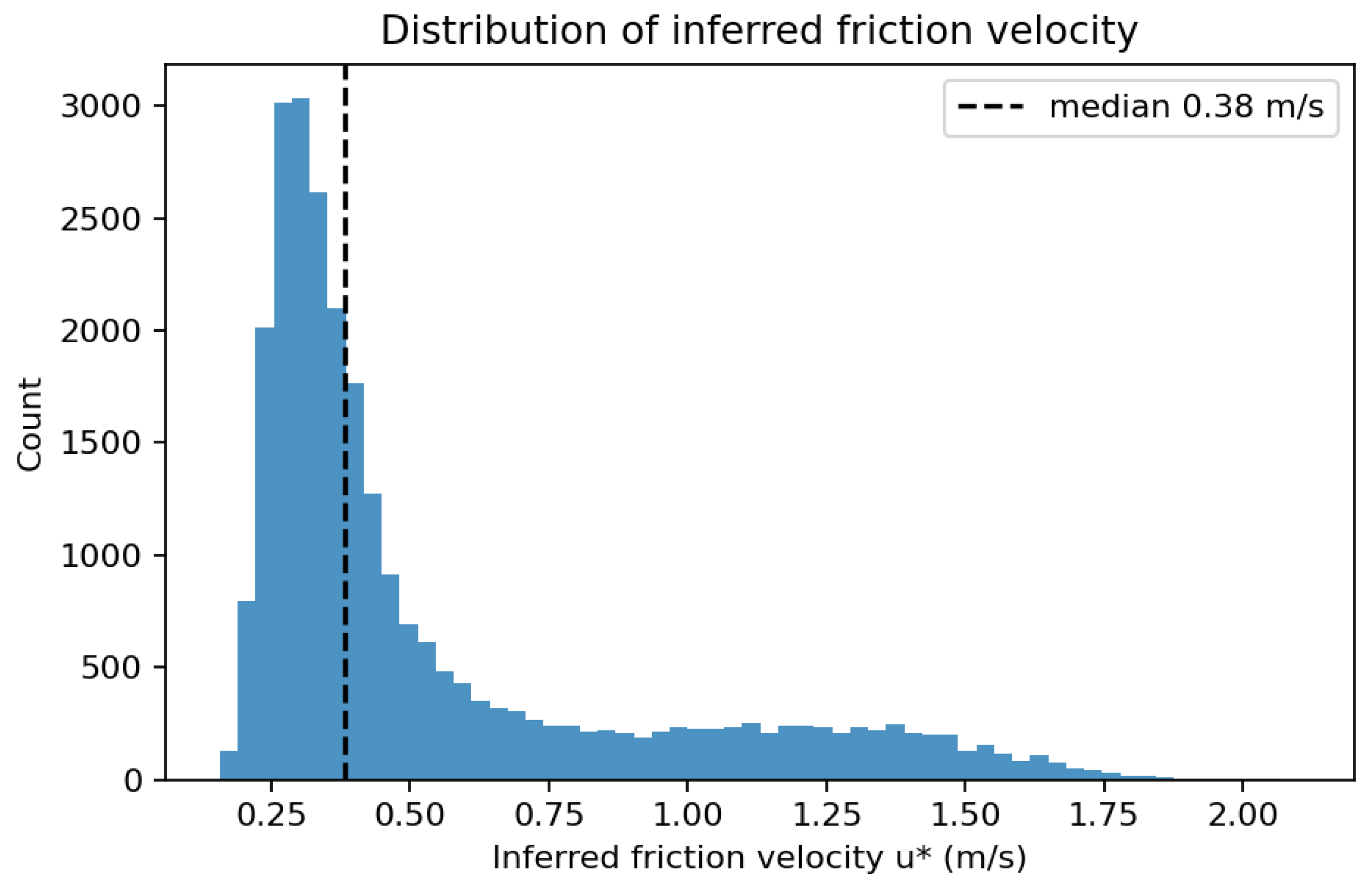
Figure 8.
Diurnal cycle of the inferred friction velocity (mean by local hour). The model recovers the expected surface-layer behavior, with a daytime convective maximum (≈ 0.80 m/s near 14:00) and a nocturnal minimum (≈ 0.38 m/s), from surface inputs alone, without being given the time of day.
Figure 8.
Diurnal cycle of the inferred friction velocity (mean by local hour). The model recovers the expected surface-layer behavior, with a daytime convective maximum (≈ 0.80 m/s near 14:00) and a nocturnal minimum (≈ 0.38 m/s), from surface inputs alone, without being given the time of day.
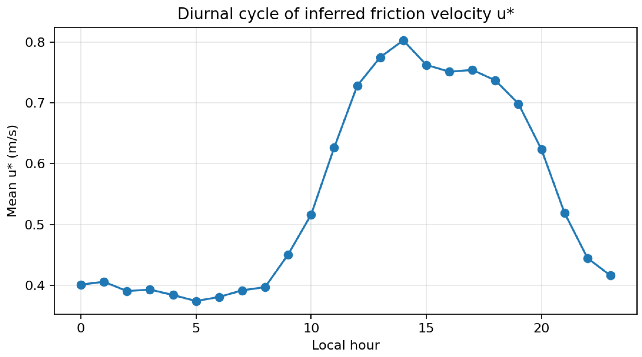
Figure 9.
Distribution of the shear exponent inferred by the shear-constrained arm’s physics head over the test set (median 0.10, mean 0.17, dashed line at the median). The median lies within the range typically reported for surface-layer wind profiles (0.1-0.4). Saturation at the upper bound (0.6) is negligible ( of samples), but of samples saturate the lower bound (0.0), predicting an essentially flat profile; whether this reflects genuinely well-mixed conditions or an unconstrained lower end of the exponent’s range is left for further investigation. enters the power-law constraint (Section 2.3.3) and is obtained without direct supervision.
Figure 9.
Distribution of the shear exponent inferred by the shear-constrained arm’s physics head over the test set (median 0.10, mean 0.17, dashed line at the median). The median lies within the range typically reported for surface-layer wind profiles (0.1-0.4). Saturation at the upper bound (0.6) is negligible ( of samples), but of samples saturate the lower bound (0.0), predicting an essentially flat profile; whether this reflects genuinely well-mixed conditions or an unconstrained lower end of the exponent’s range is left for further investigation. enters the power-law constraint (Section 2.3.3) and is obtained without direct supervision.
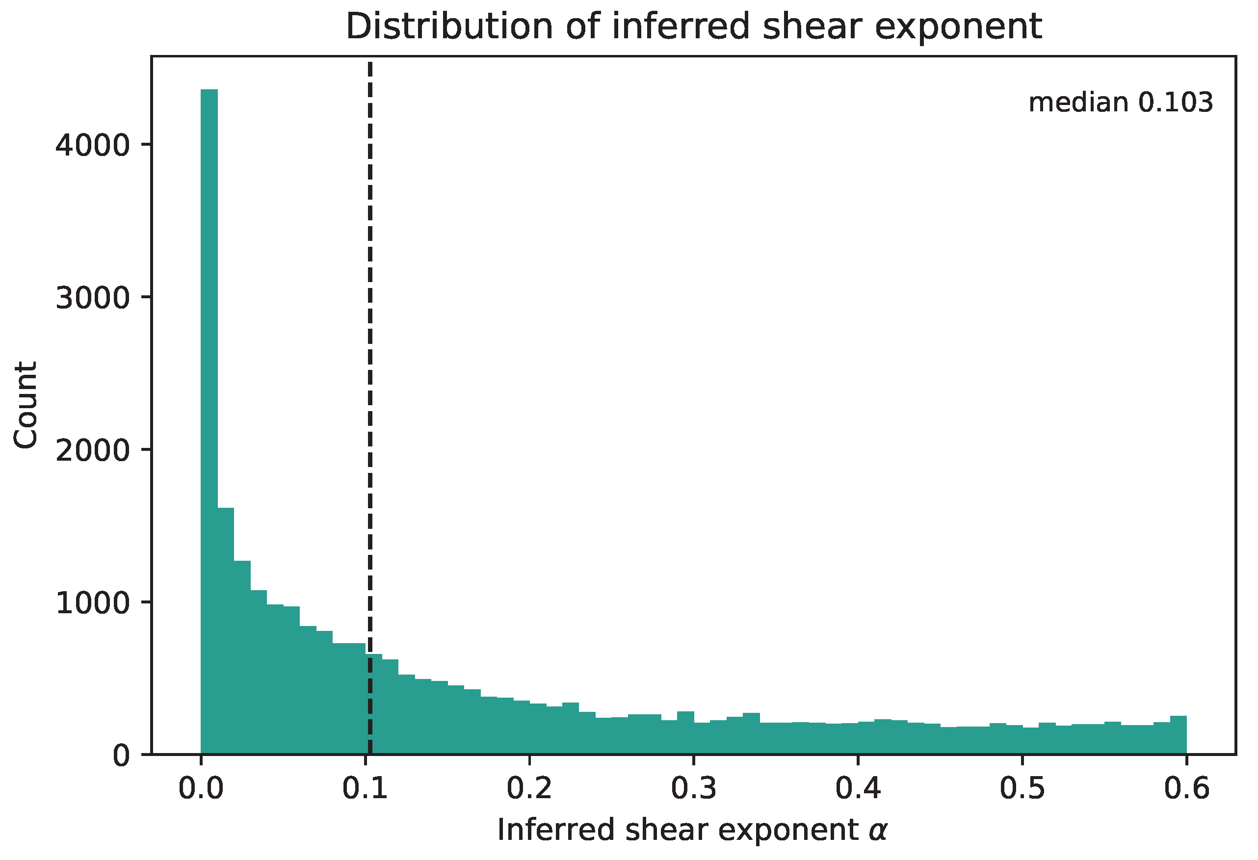
Figure 10.
Diurnal cycle of the inferred shear exponent (mean by local hour), recovered from surface inputs alone without being given the time of day.
Figure 10.
Diurnal cycle of the inferred shear exponent (mean by local hour), recovered from surface inputs alone without being given the time of day.
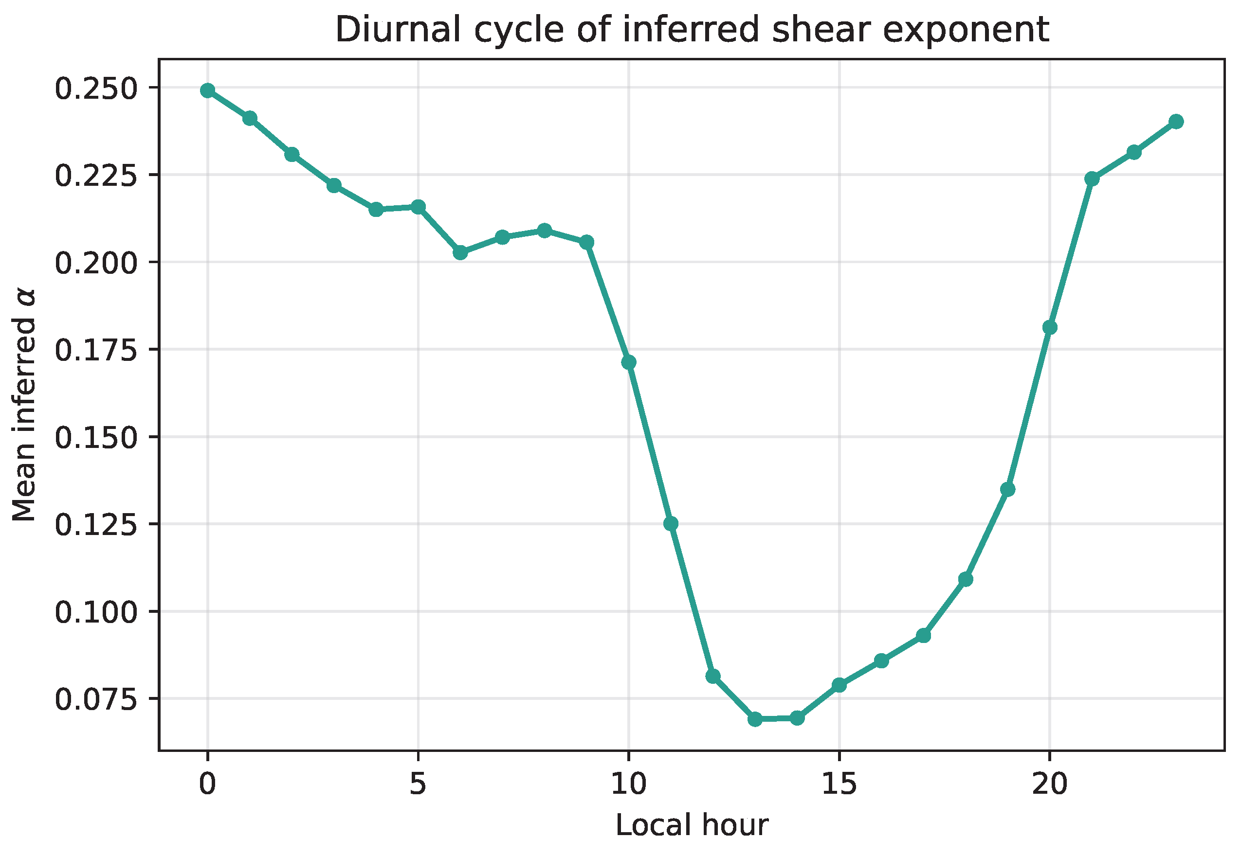
Figure 11.
Test error resolved in time, for the three architecture-matched arms. (a) Mean speed RMSE by local hour. (b) Mean speed RMSE by meteorological season. All three arms follow the same diurnal and seasonal pattern, highest at night and in winter, lowest in the afternoon and in summer.
Figure 11.
Test error resolved in time, for the three architecture-matched arms. (a) Mean speed RMSE by local hour. (b) Mean speed RMSE by meteorological season. All three arms follow the same diurnal and seasonal pattern, highest at night and in winter, lowest in the afternoon and in summer.
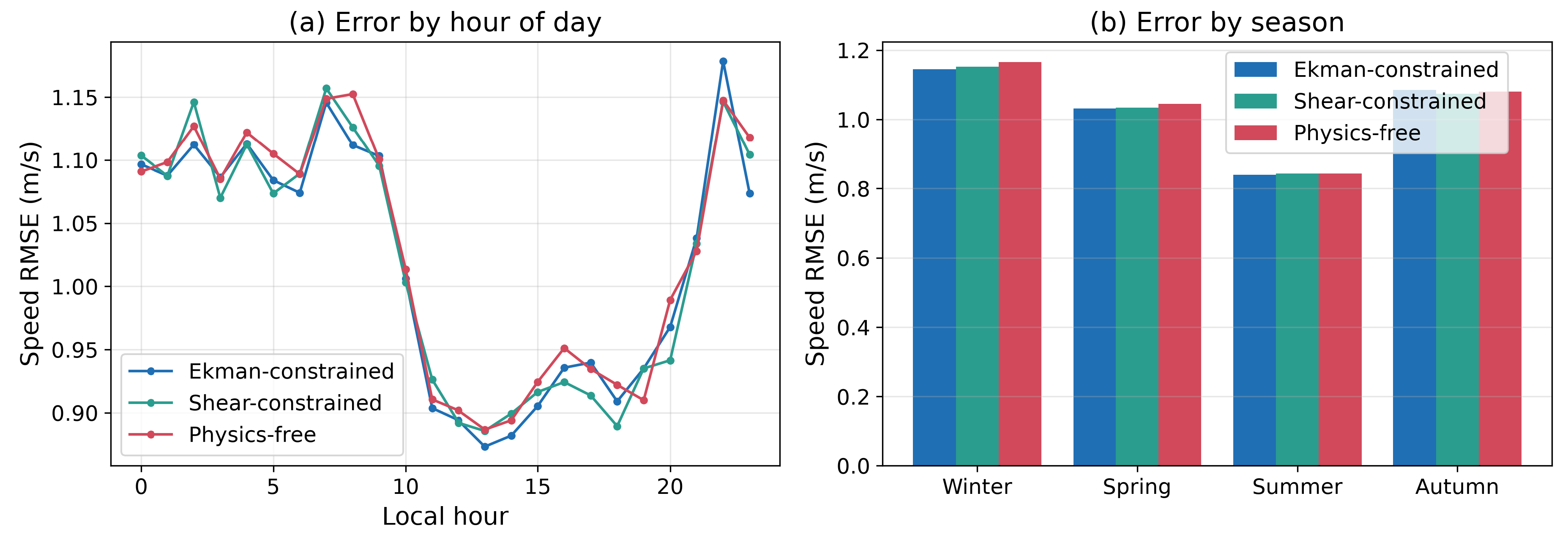
Figure 12.
Test speed RMSE by K-Means regime, for the three architecture-matched arms. The nocturnal stable regime (C0) is the hardest case for all three; the two convective regimes (C1, C2) are easier and comparable across arms.
Figure 12.
Test speed RMSE by K-Means regime, for the three architecture-matched arms. The nocturnal stable regime (C0) is the hardest case for all three; the two convective regimes (C1, C2) are easier and comparable across arms.
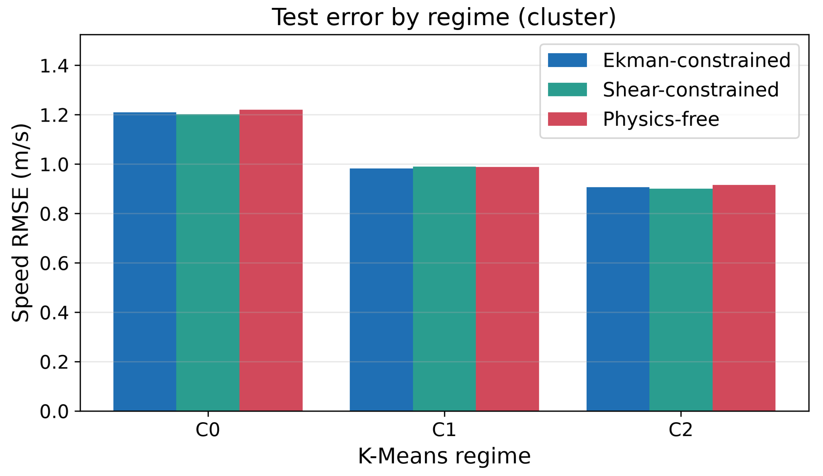
Figure 13.
Measured and predicted wind speed (top) and direction (bottom) at 100 m over a continuous nocturnal stable-regime (C0) window, for the three architecture-matched arms.
Figure 13.
Measured and predicted wind speed (top) and direction (bottom) at 100 m over a continuous nocturnal stable-regime (C0) window, for the three architecture-matched arms.
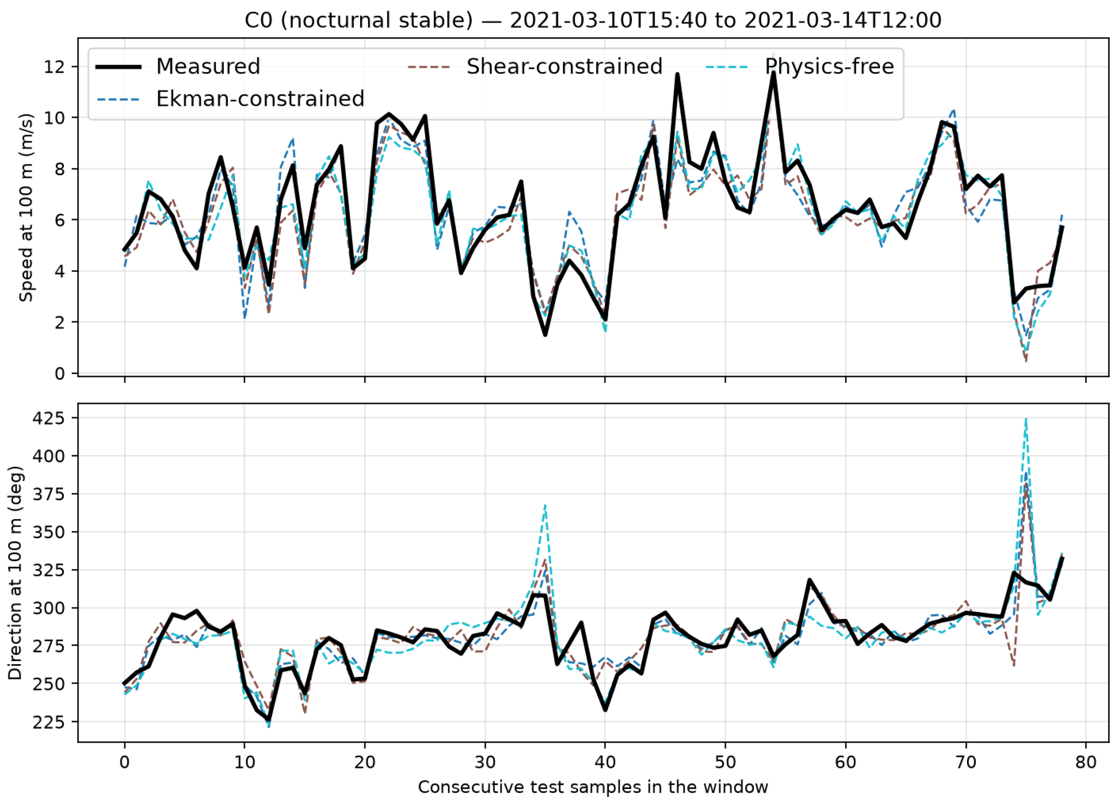
Figure 14.
Measured and predicted wind speed (top) and direction (bottom) at 100 m over a continuous convective-regime (C1) window, for the three architecture-matched arms.
Figure 14.
Measured and predicted wind speed (top) and direction (bottom) at 100 m over a continuous convective-regime (C1) window, for the three architecture-matched arms.
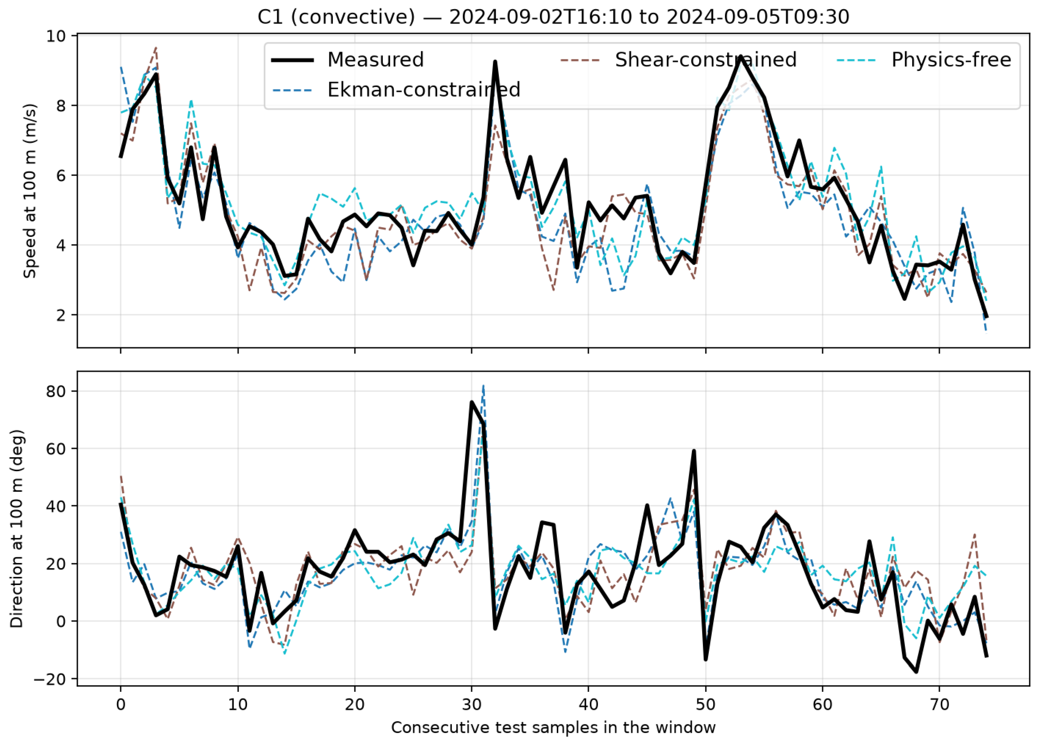
Figure 15.
Measured and predicted wind speed (top) and direction (bottom) at 100 m over a continuous convective-regime (C2) window, showing the same behavior as C1.
Figure 15.
Measured and predicted wind speed (top) and direction (bottom) at 100 m over a continuous convective-regime (C2) window, showing the same behavior as C1.
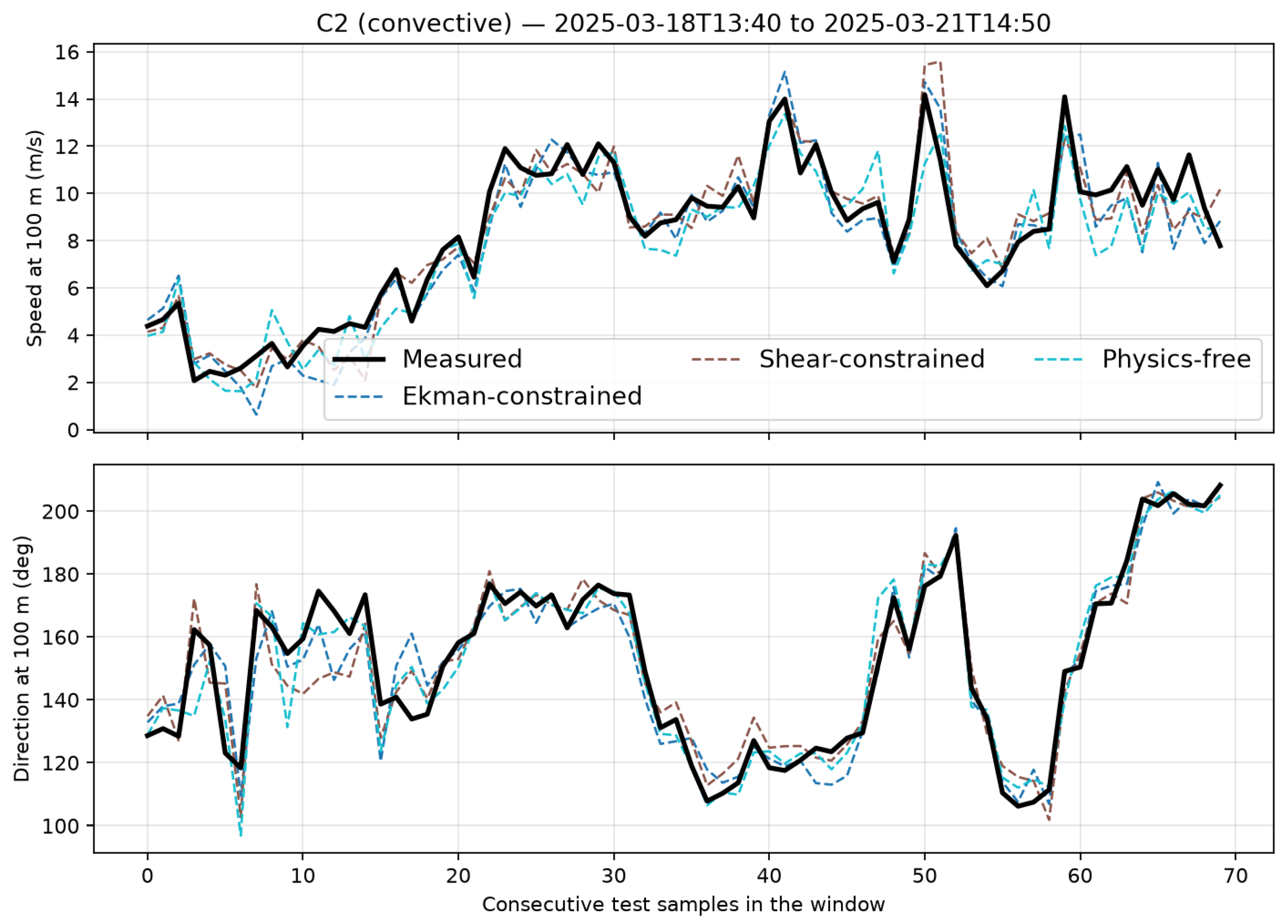
Figure 16.
Test speed RMSE (a) and direction MAE (b) versus training-set size, for the three architecture-matched arms, contiguous-month and distributed (days-per-month) sampling. Stars mark the full-record reference point. No arm is consistently better than the others at any training-set size.
Figure 16.
Test speed RMSE (a) and direction MAE (b) versus training-set size, for the three architecture-matched arms, contiguous-month and distributed (days-per-month) sampling. Stars mark the full-record reference point. No arm is consistently better than the others at any training-set size.
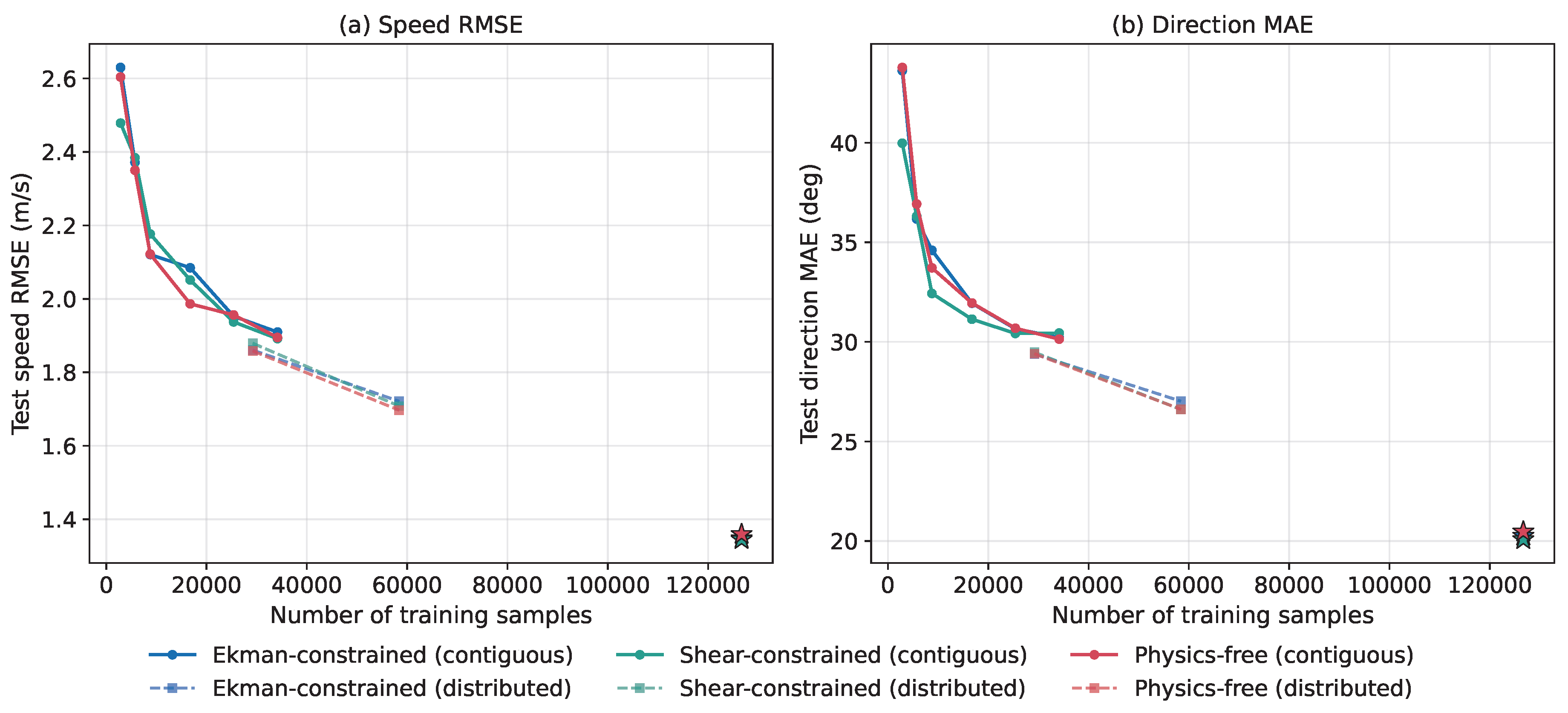
Figure 17.
Wind-speed RMSE (a) and wind-direction MAE (b) versus height. Lines: mean over four seeds; shaded envelopes: min-max across seeds. Blue: Ekman-constrained arm; green: Shear-constrained arm; red: same network, no physics. Grey region: supervised gates ( m); amber: the 140 m selection band; above: held-out test. Dashed: log law fitted on the supervised gates. Dotted vertical line in (b): , the expectation for a random bearing.
Figure 17.
Wind-speed RMSE (a) and wind-direction MAE (b) versus height. Lines: mean over four seeds; shaded envelopes: min-max across seeds. Blue: Ekman-constrained arm; green: Shear-constrained arm; red: same network, no physics. Grey region: supervised gates ( m); amber: the 140 m selection band; above: held-out test. Dashed: log law fitted on the supervised gates. Dotted vertical line in (b): , the expectation for a random bearing.
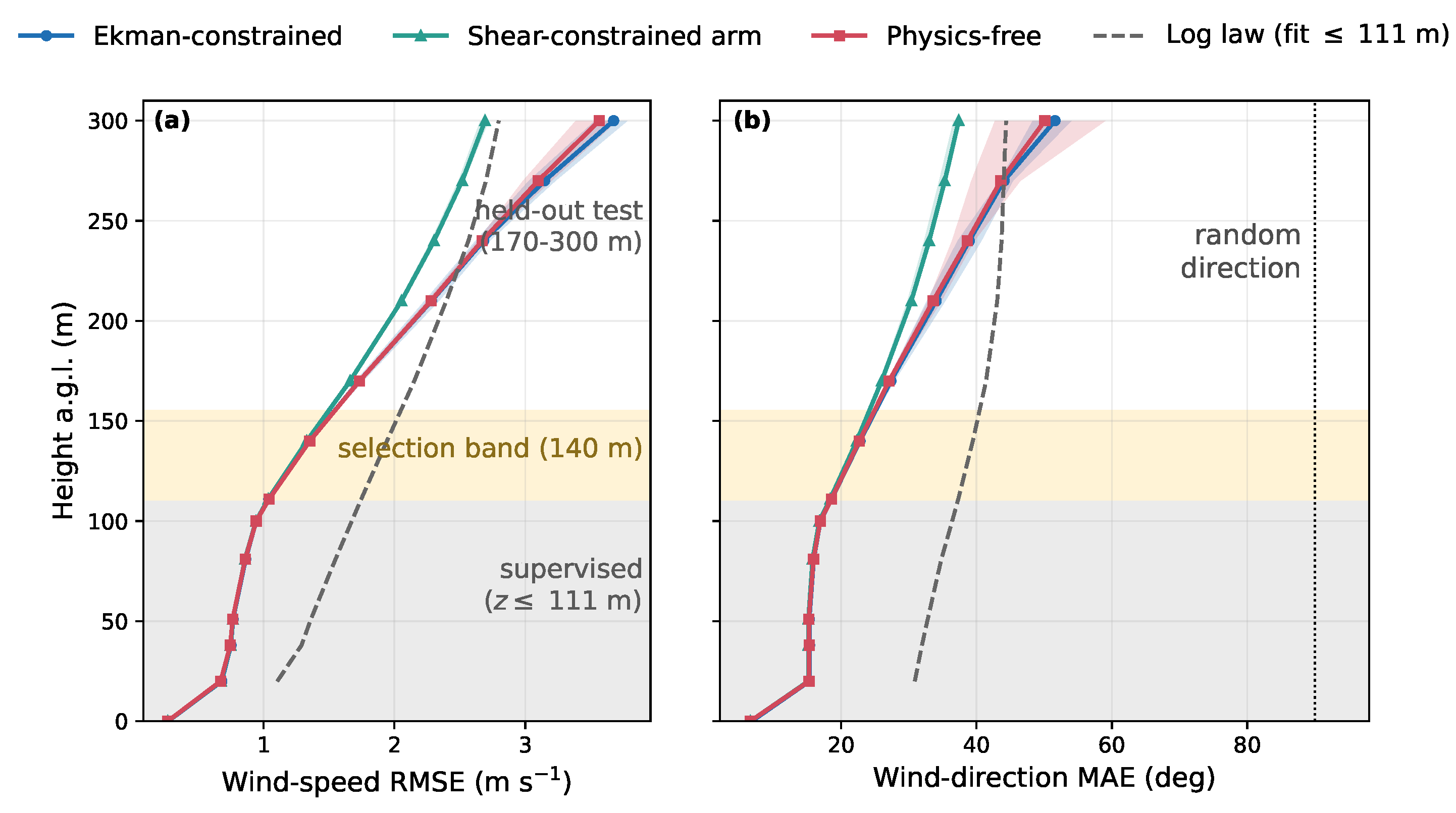
Figure 18.
Held-out-gate performance beyond pointwise error, for the Ekman-constrained arm, the shear-constrained arm, and the physics-free arm. (a) Jensen–Shannon divergence between the predicted and measured speed distributions. (b) Profile shape statistics, each normalized by its measured value, so that 1.0 (dashed line) corresponds to the measurement: curvature of the speed profile, jaggedness of the direction profile, and spread of total turning across profiles. (c) Direction MAE by K-Means regime. Bars are means over training seeds, error bars one standard deviation.
Figure 18.
Held-out-gate performance beyond pointwise error, for the Ekman-constrained arm, the shear-constrained arm, and the physics-free arm. (a) Jensen–Shannon divergence between the predicted and measured speed distributions. (b) Profile shape statistics, each normalized by its measured value, so that 1.0 (dashed line) corresponds to the measurement: curvature of the speed profile, jaggedness of the direction profile, and spread of total turning across profiles. (c) Direction MAE by K-Means regime. Bars are means over training seeds, error bars one standard deviation.
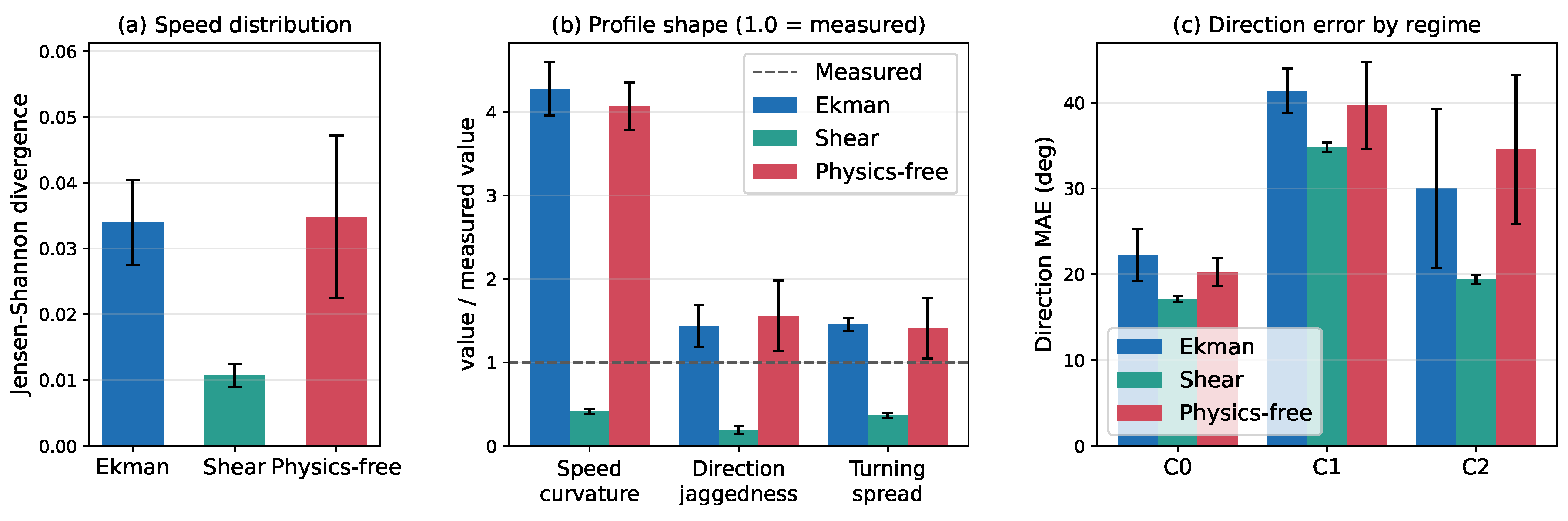

Table 1.
Hyperparameters of the three architecture-matched arms. The Ekman-constrained arm’s configuration is selected by Bayesian optimization (25 trials, 40 epochs per trial, early-stopping patience 8; the best configuration retrained for up to 120 epochs with patience 15). The shear-constrained and physics-free arms reuse this architecture rather than an independently tuned one; only the physics terms differ between the three, plus the additional output in the shear-constrained arm. Values at .
Table 1.
Hyperparameters of the three architecture-matched arms. The Ekman-constrained arm’s configuration is selected by Bayesian optimization (25 trials, 40 epochs per trial, early-stopping patience 8; the best configuration retrained for up to 120 epochs with patience 15). The shear-constrained and physics-free arms reuse this architecture rather than an independently tuned one; only the physics terms differ between the three, plus the additional output in the shear-constrained arm. Values at .
| Hyperparameter | Search space (Ekman-constrained) | Ekman-constrained | Shear-constrained | Physics-free |
|---|---|---|---|---|
|
Architecture and optimization (shared by all three) | ||||
| LSTM layer 1 (units) | 128 | 128 | 128 | |
| LSTM layer 2 (units) | 128 | 128 | 128 | |
| Decoder / dense width | 64 | 64 | 64 | |
| Context dimension | 64 | 64 | 64 | |
| Learning rate |
|
|||
| Batch size | 128 | 128 | 128 | |
| Look-back | 18 | 18 | 18 | |
| Physics terms | ||||
| Ekman weight | (log) | — | — | |
| Warm-up (epochs) | 20 | — | — | |
| anchor | 0 | — | — | |
| Surface anchor | 0.05 | 0.05 | 0.05 | |
| Shear weight | Reuses | — | — | |
| Additional output (shear exponent) |
— | absent | present | absent |
Table 2.
Aggregate in-distribution test-set performance at , every model reconstructing the full wind vector. The physics-informed arms and the physics-free arm share the architecture selected for the Ekman-constrained arm (Table 1), mean ± sd over four seeds. The classical and tree-based baselines are independent, fixed models. Models are ordered by increasing speed RMSE.
Table 2.
Aggregate in-distribution test-set performance at , every model reconstructing the full wind vector. The physics-informed arms and the physics-free arm share the architecture selected for the Ekman-constrained arm (Table 1), mean ± sd over four seeds. The classical and tree-based baselines are independent, fixed models. Models are ordered by increasing speed RMSE.
| Model | RMSE (m/s) | MAE (m/s) | JS | Dir. MAE (°) |
|---|---|---|---|---|
| Shear-constrained | 1.346 ± 0.003 | 0.818 ± 0.003 | 20.13 ± 0.05 | |
| Ekman-constrained | 1.351 ± 0.003 | 0.820 ± 0.003 | 20.21 ± 0.10 | |
| Physics-free | 1.360 ± 0.003 | 0.828 ± 0.008 | 20.39 ± 0.12 | |
| Random forest | 1.80 | 1.22 | 27.50 | |
| Power-law | 2.01 | 1.44 | 35.10 | |
| Logarithmic | 2.02 | 1.46 | 35.10 | |
| Constant | 2.97 | 2.18 | 35.10 |
Table 3.
Held-out test performance (170–300 m; genuine measurements only; 25,743 paired test sequences), all three arms sharing the architecture selected for the Ekman-constrained arm. Mean ± sd over four training seeds. The shear-constrained arm’s gain is confirmed against its own architectural control ( with the same output present but unused): m/s, m/s MAE and , matching the physics-free arm rather than the shear-constrained one.
Table 3.
Held-out test performance (170–300 m; genuine measurements only; 25,743 paired test sequences), all three arms sharing the architecture selected for the Ekman-constrained arm. Mean ± sd over four training seeds. The shear-constrained arm’s gain is confirmed against its own architectural control ( with the same output present but unused): m/s, m/s MAE and , matching the physics-free arm rather than the shear-constrained one.
| Model | RMSE (m/s) | MAE (m/s) | Dir. MAE (°) | Paired Wilcoxon vs shear-constrained |
|---|---|---|---|---|
| Shear-constrained | 1.80 ± 0.01 | 1.28 ± 0.01 | 27.0 ± 0.3 | – |
| Ekman-constrained | 2.66 ± 0.10 | 1.84 ± 0.07 | 34.2 ± 1.8 | Shear better in 65–71% of samples; |
| Physics-free | 2.61 ± 0.12 | 1.80 ± 0.07 | 33.9 ± 2.0 | Shear better in 65–68% of samples; |
Disclaimer/Publisher’s Note: The statements, opinions and data contained in all publications are solely those of the individual author(s) and contributor(s) and not of MDPI and/or the editor(s). MDPI and/or the editor(s) disclaim responsibility for any injury to people or property resulting from any ideas, methods, instructions or products referred to in the content. |
© 2026 by the authors. Licensee MDPI, Basel, Switzerland. This article is an open access article distributed under the terms and conditions of the Creative Commons Attribution (CC BY) license (http://creativecommons.org/licenses/by/4.0/).
Copyright: This open access article is published under a Creative Commons CC BY 4.0 license, which permit the free download, distribution, and reuse, provided that the author and preprint are cited in any reuse.