
Submitted:
07 September 2026
Posted:
09 September 2026
You are already at the latest version
Abstract
The rapid expansion of hydrogen production from low-carbon sources requires large-scale, flexible and reliable storage solutions to balance supply and demand and support the integration of hydrogen into future energy systems. Underground hydrogen storage, and particularly storage in salt caverns, offers significant potential due to the favourable characteristics of salt formations and the possibility of storing and recovering large quantities of hydrogen. However, identifying and comparing prospective storage sites requires the simultaneous consideration of geological suitability, uncertainty in the available data, operating characteristics, and project-specific requirements. Existing screening approaches generally address only subsets of these aspects, limiting their applicability to comprehensive site comparison and ranking. This study develops a holistic Decision-Making Tool (DMT) for the preliminary screening and comparative ranking of potential hydrogen storage sites in salt formations. The methodology integrates four complementary information categories: Static, Static-probabilistic, Dynamic, and Operator’s data. Deterministic suitability assessment, Monte Carlo-based uncertainty propagation, engineering feasibility calculations of hydrogen storage performance, and operator-defined requirements are sequentially combined into a scenario-dependent final ranking. The methodology has been implemented in an Excel-based, transparent tool, allowing multiple candidate sites and alternative storage scenarios to be evaluated without changing the underlying calculation framework. Application to three prospective evaporite areas in western Greece demonstrates the ability of the tool to distinguish between sites not only according to geological suitability, but also according to data confidence, storage performance and proximity to hydrogen production and consumption hubs. The resulting framework provides a practical bridge between early-stage geological screening and engineering-oriented site selection, while retaining the flexibility to adapt the ranking to different project objectives and levels of decision-making.
Keywords:
underground hydrogen storage
; salt caverns
; decision-making tool
; site screening
; site ranking
; uncertainty assessment
; multi-criteria decision analysis
1. Introduction
Selecting a suitable geological site is a critical early-stage decision in the development of underground hydrogen storage (UHS). A geological formation may offer substantial theoretical capacity and still be unsuitable if it cannot ensure hydrogen containment, operate safely within the required pressure range, provide sufficient recoverable working gas, or connect effectively to hydrogen production and demand centers [1,2]. Site selection must therefore extend beyond capacity estimation and compare candidate locations in terms of geological suitability, engineering feasibility and project-specific requirements, while accounting for uncertainty in the available information.
Three principal geological options are currently considered for UHS: salt caverns developed in evaporite deposits, depleted hydrocarbon reservoirs, particularly depleted gas fields, and deep saline aquifers [1,2]. Although all three geological settings can support cyclic hydrogen injection and withdrawal, their suitability depends on site- and region-specific geological, technical and economic conditions.
Among these options, salt caverns are artificial underground cavities created within thick, relatively pure salt formations and are considered particularly attractive for large-scale hydrogen storage [3]. Suitable salt formations are typically halite (rock salt) deposits with sufficient thickness, lateral continuity and depth, and with limited interbedded impurities or other discontinuities. Rock salt exhibits extremely low porosity and permeability, while its ductile behavior allows it to deform gradually under geological stresses and promotes the closure of small fractures [4,5]. These characteristics provide an excellent natural containment environment for hydrogen. The cavern must nevertheless be located at an appropriate depth: it needs to be deep enough to provide sufficient pressure and mechanical stability, but not so deep that excessive stress, temperatures or drilling and construction costs become problematic.
The cavern is created by drilling one or more wells from the surface into the salt formation, followed by a process known as solution mining or leaching [6]. Fresh water is injected through the well into the salt, where it dissolves the halite. The resulting brine is brought back to the surface through a separate part of the well system. The injection configuration and water flow are adjusted progressively to control the size and geometry of the cavern, while continuous monitoring and sonar surveys are used to verify that the required dimensions and mechanical constraints are satisfied [7]. The overall development sequence comprises site characterization and appraisal, well drilling and completion, solution mining and cavern shaping, sonar and mechanical verification, and commissioning, as summarized in Figure 1.
Following commissioning, the engineered cavern can be used for repeated hydrogen injection and withdrawal [1,2]. Unlike porous reservoirs, in which hydrogen occupies interconnected pore space, a salt cavern provides a defined storage void that can accommodate frequent cycling. Cavern operation is controlled by specified minimum and maximum pressure limits, which are established to maintain mechanical stability and restrict excessive salt deformation. The cavern pressure varies between these limits during the injection and withdrawal phase illustrated in Figure 2.
The gas retained in the cavern to maintain the minimum operating pressure is referred to as cushion gas and is not normally withdrawn during routine operation. The remaining volume constitutes the working gas and represents the recoverable hydrogen available for commercial use [8]. The selection of the cushion gas can therefore influence both project economics and the purity of the withdrawn hydrogen. Safe operation additionally requires continuous monitoring of cavern pressure and temperature, well integrity, cavern geometry and hydrogen composition. Together with the extremely low permeability of rock salt, these operational characteristics make salt caverns suitable for both high-frequency cycling and seasonal hydrogen storage. Their practical storage performance, however, is governed not only by cavern volume but also by the applicable pressure limits and the proportion of stored hydrogen that can be recovered.
These geological and operational dependencies imply that preliminary site screening must determine whether a candidate salt formation can support stable cavern development, maintain containment during repeated pressure cycling and provide sufficient working-gas capacity for the intended storage service. The screening process must therefore consider the geological and geometrical characteristics of the salt formation, the integrity of the surrounding geological setting, the anticipated operating conditions, and the maturity and quality of the available data [1,9,10,28]. The latter is particularly important because uncertainty in geological interpretation can directly affect assessments of cavern constructability, operating limits, storage capacity and containment performance.
Site selection is also not exclusively a subsurface problem. A geologically favorable salt formation may be less attractive if it cannot accommodate the required quantity of hydrogen, is incompatible with the expected gas composition, or is located far from prospective hydrogen production, transport or demand hubs. Geological suitability must therefore be considered together with engineering storage performance, infrastructure connectivity and project-specific requirements. Because these factors represent different and sometimes competing dimensions of site suitability, the selection problem is well suited to multi-criteria decision-making (MCDM).
Previous research on underground hydrogen storage has established foundational insights into the geochemical, geomechanical, and techno-economic factors driving site selection. Early studies focused heavily on the halite content of host formations, as well as the complex interactions between hydrogen, cushion gas, and microorganisms, demonstrating their critical role in injection-withdrawal cycles and containment integrity [1,2,11,12,13]. Beyond these localized biochemical mechanisms, broader geomechanical stability has been extensively investigated; local tectonic regimes, fault networks, and seismicity directly dictate sealing efficiency and infrastructure safety [9,14,15,16]. Additionally, techno-economic parameters—most notably geographic proximity to both hydrogen producers and end-consumers—heavily influence the final market price of the delivered gas [17]. Synthesizing these insights, recent efforts have focused on developing comprehensive roadmaps to guide optimal site selection among competing geological candidates.
In a comprehensive review of large-scale underground energy storage, Matos et al. (2019) established a baseline roadmap to define desirable formation characteristics for UHS in both salt caverns and porous media [18]. Although the authors did not provide a structured site-screening tool, they introduced critical threshold values, including operational depth windows and minimum halite content. To build a structured prioritization framework, Nemati et al. (2019) developed a comprehensive decision-making model using the Fuzzy-Delphi method [19]. Through systematic literature screening, the authors extracted 18 sub-criteria across technical, economic, and environmental dimensions to form an expert questionnaire which was then statistically analyzed to gain results. While this framework successfully captures macro-level sustainability and regulatory factors, it remains a qualitative decision-making measure that does not integrate granular, deterministic technical data.
To bridge the gap between abstract models and field applications, the Hystories project compiled geological data by adapting established operational parameters from natural gas storage and applying them directly to underground hydrogen storage (UHS) [10]. In contrast to the purely qualitative approach of Nemati et al. (2019), the Hystories framework assigned explicit quantitative ranges to critical parameters, such as defining operational minimum and maximum depth boundaries. Additionally, the project introduced robust screening (exclusion) criteria, such as eliminating highly faulted locations, alongside scoring criteria like optimal reservoir thickness. However, the project did not synthesize these isolated criteria into a single, unifying equation capable of generating a definitive suitability rank for a given candidate site. Furthermore, its site-selection thresholds remain strictly limited to porous media, leaving a gap for broader, multi-formation screening frameworks.
Allsop et al. (2023) utilized a traffic-light indexing system to evaluate Zechstein Group salt formations in the Southern North Sea for hydrogen storage, assigning numerical scores (10, 5, 1) based on geological and engineering criteria while applying a 50% capacity reduction for conservative estimation [9]. Site selection required validation via legacy seismic data and historical boreholes, yet the methodology was limited by an absence of an explicit, unified scoring formula and the application of equal weight to all criteria.
Huang et al. (2024) developed a multi-criteria site evaluation framework for underground hydrogen storage in bedded salt formations using the Analytic Hierarchy Process (AHP), prioritizing factors like halite purity and proximity to infrastructure via bibliometric analysis [20]. The methodology, which weights expert-defined scores to determine site suitability, is tailored for the specific interlayer characteristics of the Pingdingshan field. Because of this focus on thin-bedded formations, applying the model to massive salt domes requires substantial recalibration to address the different geological constraints.
Shifting focus to dome structures, Maraggi and Moscardelli (2024) developed an engineering-based evaluation tool calibrated for onshore and offshore salt domes within the Gulf of Mexico basin [21]. Their framework executes detailed volumetric calculations alongside operational modeling for hydrogen production, injection, and cycling scenarios. Specifically, the tool computes critical engineering metrics, including the maximum permissible cavern count, localized storage capacities, gas flow rates, and working gas requirements. However, this model does not feature an automated site-screening or ranking capability; instead, it generates raw deterministic outputs that can be manually integrated into secondary screening procedures.
To overcome the high computational costs associated with traditional numerical reservoir simulation, Malki et al. (2024) developed a user-friendly site optimization tool tailored for porous media [22]. Their framework utilizes artificial neural networks (ANNs) as a reduced-order model (ROM), which was trained on outputs from extensive numerical simulations. The model integrates key geological and operational parameters, including depth, formation thickness, injection pressure coefficients, and bottom-hole pressures. By streamlining these variables into an optimized framework, the tool enables users to evaluate long-term site evolution under varying injection strategies, quantify operational uncertainties, and perform robust parameter sensitivity analyses.
Building directly upon the Hystories project database, Lankof et al. (2024) developed a dedicated selection framework for porous media using the Analytic Hierarchy Process (AHP) [23]. Their methodology applies 10 exclusionary criteria—such as storage areal extent, depth, and the availability of seismic surveys—to filter out unsuitable candidates, followed by nine scoring criteria including reservoir thickness, depth, and lithology. To enhance the robustness of their scoring results, the authors incorporated weighted factors derived from two distinct deterministic approaches: expert judgment and the Entropy Weight Method (EWM). Similarly, Harati et al. (2024) established a ranking methodology for UHS in porous media by combining AHP with expert knowledge to assign weights to eight selected technical and economic criteria [24]. To determine the final site prioritization, they integrated the Preference Ranking Organization Method for Enrichment Evaluations (PROMETHEE) to rigorously evaluate and compare the alternatives against each criterion.
To formalize site-suitability assessments, Borghini et al. (2025) proposed a structured screening framework based on a defined set of geological parameters [25]. Their model evaluates caprock integrity (porosity, lithology, and thickness), reservoir quality (porosity and permeability), and macro-level site characteristics (temperature, salinity, and depth). Each parameter is evaluated using a score-based system ranging from 0 (unsuitable) to 5 (suitable) depending on its measured value. These scores are then aggregated to calculate three independent metrics: the caprock potential index, the reservoir quality index, and the site potential index. Finally, these sub-indices are integrated into a single governing equation to yield a comprehensive UHS suitability index, which defines the overall feasibility of the candidate site.
To assess massive halite deposits, Blancone et al. (2025) evaluated the hydrogen storage potential of the Zechstein Group for salt cavern development [26]. However, their work outlines an early-stage screening workflow rather than a structured multi-criteria decision-making tool. The authors utilized a combination of seismic, well, and core data to identify potential regions, mapping key characteristics such as depth, areal footprint, salt structure morphology, and caprock thickness. These parameters were subsequently compiled into a Geographic Information System (GIS) database. By coupling this spatial data with the GeoH2 tool developed by [21] to calculate storage capacities, and overlaying it with data density and structural symmetry maps, they classified regions into low-, moderate-, and high-risk zones to assist in preliminary site screening.
Advancing GIS-based evaluation frameworks, Anzelmo et al. (2026) adopted the Common Risk Segment (CRS) approach to assess potential storage sites [27]. Their model integrates 20 distinct parameters categorized by salt formation characteristics (e.g., structural complexity), macro-geological constraints (e.g., caprock integrity, for a review see [28]), and environmental risks (e.g., seismicity). The final score for each candidate site combines parameter importance, individual parameter scores, and localized data confidence levels to generate composite risk maps within a GIS environment. To test ranking stability, the authors executed a Monte Carlo sensitivity analysis by perturbing data confidence levels using a uniform distribution. However, their framework neglects critical hydrogen-specific biochemical factors, such as microbial activity or hydrogen-rock geochemical interactions. Furthermore, relying exclusively on a uniform distribution oversimplifies the variance of variables like halite content or infrastructure availability, which inherently follow distinct statistical distributions. In a parallel GIS-based study, Garvey et al. (2026) developed a spatial screening framework to map sites and estimate their theoretical storage potential [29]. Their methodology overlays an independent hexagonal grid across each site to perform localized calculations within individual grid blocks. Suitability index maps are then derived by assigning weighted scores and impact factors across 19 criteria. While this approach provides valuable insights into spatial suitability variations, it focuses heavily on surface facilities and environmental factors, leaving critical subsurface geological constraints under-evaluated.
However, a prominent methodological gap persists across the current state-of-the-art: the majority of screening models lack both geological universality and statistical flexibility. While a significant portion of literature focuses on porous media cases to the exclusion of evaporitic systems, the sparse frameworks designed for salt caverns suffer from geographic over-customization, binding their criteria to regional formations like the Zechstein Group or the Pingdingshan bedded salt field. Consequently, these models lack the adaptability required for generalized cross-formation or salt-dome screening. Furthermore, the reliance on rigid, deterministic parameters to weight screening criteria remains a major limitation. This deterministic bias fails to account for the stochastic uncertainties, variable data confidence, and subsurface heterogeneities typical of prospective storage sites, underscoring the urgent need for more robust, probabilistic site-evaluation methodologies.
To address the gap identified above, the present study develops a holistic integrated Decision-Making Tool (DMT) for the preliminary screening and comparative ranking of potential UHS sites in salt formations. The framework draws on four categories of information: static site data, probabilistic information describing confidence in the static criteria, dynamic cavern and operating data, and operator-defined requirements. These inputs are processed through a sequential assessment workflow. First, a deterministic site-suitability assessment evaluates each candidate using eight predefined static criteria. Second, a stochastic assessment employs Monte Carlo simulation to propagate uncertainty in the confidence assigned to these criteria and examine the robustness of the resulting site assessment [30]. Third, an engineering feasibility assessment uses an Equation of State to calculate hydrogen storage capacity, fill factor and recovery factor under the specified cavern and operating conditions [31]. Finally, the suitability and engineering indicators are combined with operator-defined requirements, including the target storage quantity and distances from hydrogen production and consumption hubs, to produce a scenario-dependent comparative ranking. The methodology is implemented in an Excel-based interface that retains the intermediate inputs and outputs, thereby providing a transparent, repeatable and traceable screening process.
The developed DMT is intended to support comparative decision-making during preliminary site screening rather than to replace detailed geological characterization, geomechanical modelling, dynamic reservoir simulation or project-specific techno-economic assessment. To demonstrate its application, the methodology is applied to three candidate evaporite areas in western Greece, Filiates, Astakos and Zante, to examine how geological suitability, confidence in the available data, calculated storage performance and infrastructure proximity influence their relative ranking.
The remainder of the paper is organized as follows. Section 2 describes the principal components and input categories of the DMT. Section 3 presents the proposed methodology, including the deterministic, stochastic and engineering calculations together with the final ranking procedure. Section 4 describes the implementation of the DMT in the Excel-based user interface. Section 5 introduces the three study areas, applies the proposed methodology and discusses the resulting site rankings. Finally, Section 6 summarizes the main conclusions and limitations of the proposed framework.
2. The Components of the DMT
2.1. Screen/Ranking Data Sources
A holistic approach to site screening and ranking must consider information beyond the geological setting, including site-specific parameters such as the minimum and maximum allowed operating pressures, total hydrogen storage capacity that can be accommodated by the cavern system, the composition of the H2 stream intended to be stored, including the presence of impurities, and the distances to hydrogen production and consumption hubs. Together, these parameters affect the technical feasibility, storage performance, infrastructure integration and economics of the storage project and, therefore, influence its attractiveness and progression towards a final investment decision (FID).
The approach proposed in this work integrates four distinct data categories, each comprising categorical and/or numerical inputs. The first category comprises geological information, which, despite being subject to inherent uncertainties, provides the primary basis for the initial screening of potential storage sites. Among others, the relevant criteria include lithology, tectonic setting, and the prevailing stress state. Although these criteria may have different levels of influence on the final assessment, they all must be considered. This data category is hereafter referred to as “Static”, in the sense that it describes intrinsic site characteristics that are treated as fixed inputs during a given screening exercise and are not expected to vary with the selected operational scenario.
The second data category represents the uncertainty associated with each Static criterion. Simple representation of the data confidence (e.g., by assigning a “Low”, “Medium”, “High” value) or a real probabilistic approach utilizing distributions for each parameter involved is an essential part of this approach. This data category is hereafter referred to as the “Static-probabilistic”.
Additional site characteristics, primarily associated with storage and withdrawal operations, must also be taken into account. These include the number of caverns that can be operated simultaneously, the extent to which leaching can produce caverns of sufficient volume, and the potential requirement for cushion gas to maintain operational pressure. The minimum and maximum allowable pressures, together with temperature, are also essential parameters in this assessment. This group of inputs is hereafter referred to as “Dynamic”, since they vary over time.
Finally, “Operator’s” requirements are considered. These are generally independent of the geological characteristics of the salt caverns and instead reflect the intended operational configuration of the storage site. The total quantity of H2 expected to be stored in the caverns is a fundamental parameter for ranking candidate sites. The presence of impurities is relevant to the thermodynamic properties of the hydrogen stream and, consequently, to the mass that can be stored and recovered under the specified operating conditions. Similarly, the distances from the hydrogen producer to the storage site and from the storage site to the final consumer are included as important criteria.
In the following Sections, the individual criteria associated with each data category are presented in detail and are subsequently combined to obtain the desired site-screening and ranking results.
2.2. Site Static Data
The Static data describe the intrinsic geological, structural, integrity-related and operational-readiness characteristics of each candidate site. Eight Static criteria are considered: lithology, salt structure, tectonics, depth, field status, microbial processes, stress state and seismicity. Together, these criteria provide the basis for the initial assessment of whether a site is suitable for further engineering and operator-oriented evaluation.
2.2.1. Lithology
The preferred host formation for salt caverns is high purity halite without heterogeneities such as intercalated layers or fragments of anhydrite, claystone, mudstone or K-Mg salts [4,32]. Such heterogeneities constitute insoluble material that accumulates at the bottom of the cavern after leaching, thereby occupying valuable storage space. Impurities can also affect the leaching process resulting in an asymmetrical distribution of storage space and potentially affecting the geomechanical stability of the caverns. Moreover, thin bedding, alternating layers of salt and non-salt material, or brecciated salt should be avoided, if possible, as stability and thus integrity issues may arise from the injection/withdrawal cycles [4,15,33]. Historically, technical experience has indicated that the proportion of insoluble material should ideally remain below approximately 25–30% of the total salt rock [34,35]. However, recent research demonstrates that successful cavern leaching may remain geomechanically viable in formations where the insoluble percentage may reach up to 40%, thereby expanding the available site options [5].
2.2.2. Salt Structure
Salt deposits may occur as domes, breccias, or thick/thin-bedded layers within the evaporitic formations. The most desirable structural setting for geological storage is a salt dome, which typically exhibits homogeneous lithology, both vertically and horizontally, and a comparatively uniform stress distribution [36]. Salt dome structures along with thick bedded salt are preferable from a geotechnical perspective because they allow caverns to be fully enclosed within the salt, thereby [37]. By contrast, thin-layered or brecciated salts should be avoided. In the latter cases, construction and maintenance challenges may arise due to differential deformation between layers of different thicknesses, the difficulty of maintaining optimal cavern geometry, and the risk of damage to downhole equipment [36,38,39].
2.2.3. Tectonics
Faults and fractures are undesirable when developing underground facilities, particularly caverns, due to risks to both geomechanical stability and containment [15]. If an evaporite rock formation is tectonized, fractures and fissures may act as preferential flow paths for hydrogen migration. Additionally, the existence of faults or fault zones may imply an anisotropic stress regime that, in extreme cases, can even cause cavern collapse. The presence of faults in the vicinity of a cavern may result in differential displacement between the footwall and hanging wall [40], thus compromising cavern stability. Moreover, the presence of faults may promote the expansion of the plastic zone and increase the induced strains during an earthquake [41]. Active faults should be treated with particular caution, since they can be reactivated by seismic activity and affect storage integrity [42].
2.2.4. Depth
Salt caverns are typically constructed at depths ranging between 500 m and 2,000 m as the stored volume and energy are maximized within this interval [43,44,45]. Additionally, the cavern stability is significantly enhanced within this depth range [1,34,36].
Salt caverns can also be constructed at shallower or greater depths, from approximately 300 m down even to 2,700 meters. However, at depths shallower than 500 m, the working gas capacity that can be stored is low due to pressure limitations, while at depths exceeding 2,000 m, the cushion gas requirements to maintain operational pressures increase, potentially introducing additional geomechanical and structural-stability challenges [46,47].
2.2.5. Field Status
Salt cavern storage sites are characterized by different levels of development readiness and may be classified as operational, under development, or undeveloped. The timeline for administrative procedures, exploration, leaching, and surface facility installation is inherently long [10]. Solution mining alone may require a long period of time depending on cavern size, salt purity, and technical challenges. Consequently, under urgent demand scenarios, a mature or operational site may represent a more immediately feasible option.
2.2.6. Microbial Processes
Microbial presence at a UHS salt cavern site is highly undesirable as specific hydrogenotrophic species can consume the stored hydrogen leading to gas loss and contamination through undesirable by-products such as H2S [12,48]. However, the high salinity environment of a cavern is generally hostile to these microorganisms because it commonly lacks nutrients; consequently, their potential impact remains uncertain and site-dependent [49,50]. When microbial contamination does occur, it is primarily introduced through water used during leaching, workovers, well testing and previous cavern operations, or through microorganisms already present in the salt formation [51]. To counteract such contamination, various sterilization and mitigation techniques have been proposed, including chemical treatment, hot-water injection and an increase in the sump pH [49]. Any such process may increase operational and, ultimately, end-user costs; therefore, appropriate prevention and mitigation measures are required to minimize the effect on storage efficiency [42].
2.2.7. Stress State
Salt formations exhibit complex viscoelastic behavior and undergo creep deformation, which can result in nearly equal stresses in all directions and an approximately isotropic state once diapiric movement has ceased [52,53]. This behavior contributes to the formation’s plasticity and high resistance to fracturing, although it must be noted that isotropic conditions are found primarily within the central parts of a salt dome, while its edges may exhibit stress anisotropy [43,44,54]. Anisotropic regions are highly prone to crack opening, which increases the risk of sealing and containment failure under cyclic loading [55]. As a result, the area where caverns are to be leached should be investigated to determine the prevailing in-situ stress conditions.
2.2.8. Seismicity
Salt caverns, like all underground constructions, are susceptible to damage due to seismic-wave propagation. Consequently, areas of high seismicity or with a documented history of high-magnitude earthquakes should be avoided. For underground storage caverns, earthquake duration and peak ground acceleration are among the most critical determinants of long-term structural stability [56]. Studies of the seismic performance of salt caverns under compressed-CO2 storage conditions have demonstrated that thicker salt-rock layers may experience smaller displacements and induced stresses during seismic events [16]. These findings indicate that greater structural homogeneity and the absence of non-salt interlayers can contribute to enhanced stability and reduced cavern deformation. However, recently developed numerical models indicate that, under severe seismic loading associated with earthquakes of magnitude 7 or greater, both homogeneous salt caverns and those containing interlayers may present a substantial risk of structural failure [16].
2.3. Static-Probabilistic Data
Since early-stage site screening often relies on incomplete or uneven information regarding the geological setting, a stochastic uncertainty assessment needs to be incorporated into the calculations workflow. A confidence category is assigned to each criterion and then mapped to a numerical value. The higher the value, the more weight is put on that specific criterion as the confidence to its category is high as well.
A more sophisticated approach is also implemented in this work where a probability distribution is assigned to the confidence associated with each Static criterion rather than a flat value. The Monte Carlo procedure, conceptually similar to probabilistic reserves calculations [30], is then used to examine the sensitivity of the site score to uncertainty in the confidence assigned to each criterion. Standard distributions, including normal, lognormal, triangular, and uniform, can be used to describe uncertainty of an input by defining the corresponding statistical parameters, such as the mean, standard deviation, mode, and admissible bounds. The exact parameters required to define each distribution are summarized in Table A1 of the Appendix.
The deterministic confidence value defined above is used as the central reference (i.e., mean or mode), while lower and upper bounds define the admissible range of sampled confidence values. Once the distributions and their parameters are defined, the operator can run Monte Carlo simulation and receive the site score cumulative probability curves. This allows the quantification of the uncertainty associated with the available information by examining the cumulative probability curves and assessing their effect on the resulting site score.
2.4. Site Dynamic Data
The amount of hydrogen that can be stored within a cavern depends on the effective cavern volume and on the thermodynamic properties of the stored gas at the corresponding pressure and temperature conditions. Consequently, the physical cavern volume alone cannot be directly translated into hydrogen storage capacity. As a result, factors such as the achieved leaching fraction, cavern geometry, temperature, and geomechanical constraints, including the maximum and minimum allowable operating pressures, must be considered.
The data required in this group are numerical inputs representing the physical and operating characteristics of the cavern system and are used directly in the engineering-feasibility calculations.
2.4.1. Caverns Capacity Data
For each cavern, the effective storage volume is derived from the designed maximum cavern volume and the corresponding leaching fraction which depends on the success of the leaching process. Since salt caverns are artificially developed through solution mining, the entire geometrically available salt volume may not be fully converted into effective storage space due to the presence of geological heterogeneities, cavern-shape restrictions, drilling problems, spacing requirements and operational limitations [5,21].
Once the maximum operating pressure has been set (see 2.4.2), it is considered together with the cavern temperature in an Equation of State model to estimate the gas compressibility factor [31,57]. The compressibility factor is subsequently used through the real-gas relation to calculate gas density and, consequently, the maximum hydrogen mass that can be accommodated by the available cavern volume. As a result, caverns with identical geometrical volumes may provide different mass-storage capacities when operated under different pressure and/or temperature conditions. When a large-scale project is under consideration, many clusters could be utilized, each developed in its own number of caverns while honoring restrictions like appropriate spacing and operational dynamics. In such case, the total storage capacity also depends on the number of caverns assigned to each cluster.
2.4.2. Geomechanical Issues
The amount of gas that can be accommodated within a given cavern is strongly dependent on the maximum allowed storage pressure which is not a universal value but depends on the depth and geomechanical conditions prevailing in the storage formation, including lithostatic state and in-situ stress fields [36,43,47,55]. The operating hydrogen pressure must remain sufficiently below the limit at which cavern integrity could be compromised. This limit is influenced by salt depth, thickness, mechanical properties and creep behavior, as well as the cavern’s proximity to the roof and boundaries of the salt formation. The maximum operating pressure is normally established through a site-specific geomechanical assessment rather than by applying a single pressure limit to all salt caverns.
On the other hand, the minimum operating pressure of a salt cavern is primarily required to maintain cavern stability and prevent excessive deformation or convergence of the surrounding salt. In hydrogen storage, this pressure is typically maintained by a cushion gas inventory, which ensures that the cavern pressure does not fall below a site-specific lower limit during withdrawal. It therefore represents an important constraint on the usable storage capacity: a higher minimum pressure increases the amount of cushion gas required and reduces the quantity of gas that can be withdrawn for commercial use, whereas an excessively low pressure may compromise cavern integrity and accelerate salt deformation. Once the minimum operating pressure has been specified, the corresponding cushion-gas mass can be calculated using an Equation of State.
Together, the maximum and minimum operating pressures define the allowable operating window of the cavern and affect both the gross storage capacity and the recoverable working-gas quantity. These pressures are introduced into the DMT as site-specific inputs and must be established through an appropriate geomechanical assessment.
2.5. Operator’s Data
The Operator’s data define the intended storage scenario and infrastructure context against which each candidate site is evaluated. These inputs complement the Static, Static-probabilistic and Dynamic datasets and include the project-designed storage quantity, the composition of the injected gas stream and the distances to potential hydrogen production and consumption hubs. Unlike intrinsic site properties, these inputs are scenario-dependent and may vary according to the requirements of the operator and the storage project.
2.5.1. Project-Designed Storage Quantity
The operator specifies the total quantity of hydrogen that the cavern system is required to accommodate. This requirement is compared with the calculated storage capacity of the candidate site during the engineering-feasibility assessment. A site may therefore satisfy the geological screening criteria but remain unsuitable for a specific project if its available cavern capacity is insufficient to meet the predefined storage target.
The project-designed storage quantity is also used to determine the fraction of the available cavern capacity that would be utilized. Beyond satisfying the required storage quantity, the assessment therefore also considers how effectively the available cavern capacity is utilized under the selected storage scenario. To ensure a consistent comparison, the same storage target should be applied to all sites evaluated within a common ranking scenario.
2.5.2. Presence of Impurities
When impurities are present in the stored stream, its composition affects its thermodynamic behavior and density to a greater or a lesser extent. Although hydrogen represents the principal component of the stream, the presence of impurities may alter its molar mass and density and, consequently, the mass that can be accommodated under specific pressure and temperature conditions [57].
An appropriate Equation of State model is therefore used once the composition of the injected stream is defined by the operator. Hydrogen and additional mixture components can be introduced through their respective molar fractions, with the sum of the stream composition equal to unity. EoS calculations applied both at the maximum storage pressure and at the cushion-gas pressure provide the gas density under these limiting conditions, allowing the gross stored mass, cushion-gas requirement and recoverable working-gas quantity to be calculated [8,57].
2.5.3. Distance to H2 Hubs
The geographical location of a potential underground storage site relative to hydrogen production and consumption centers is an additional factor affecting its attractiveness. Even when a geological formation presents favorable storage characteristics, long transportation distances or limited access to existing or planned infrastructure may reduce its suitability for integration within a hydrogen value chain.
Two independent distance relationships are therefore considered by the DMT: the distance from the hydrogen producer to the storage site and the distance from the storage site to the final consumer. The two directions are treated independently as they describe different parts of the hydrogen transportation chain.
Rather than introducing a detailed transportation-cost model, although such a model could be incorporated, at this early screening stage, distances are classified into predefined categories which in turn get converted into numerical scores. Direct access to relevant transportation infrastructure, such as ports and pipelines, is also represented explicitly. For the site-to-consumer connection, proximity to an airport can additionally be introduced within the corresponding infrastructure category.
The resulting producer-to-site and site-to-consumer scores are incorporated into the final ranking as independent criteria. Their respective importance can be modified by the operator according to the characteristics of the storage project under investigation. Together with the designed storage quantity and gas-stream composition, these distance indicators allow each candidate site to be evaluated against a consistent operator-defined scenario. The relationship between the described data sources is illustrated in Figure 3.
3. Methodology
3.1. Deterministic Storage Site Suitability Assessment
This first methodological stage converts the Static inputs into both a screening decision and a deterministic suitability score which allows for the ranking of the sites that satisfy the screening requirements. The DMT evaluates the suitability of each candidate site using the eight Static criteria defined in Section 2.2.
For a specific storage site, three distinct inputs are introduced per criterion : a category , a confidence level and an importance weight , where the “Crit” superscript stands for “criterion”. Firstly, is a categorical variable which depicts the user-selected category for criterion out of the predefined available ones for that criterion, collectively denoted by . For example, for the Lithology criterion, a site characterized by high halite content of at least 90% is assigned to = “Pure”, out of the available = {“Pure”, “Fair”, “Tolerable”, “Rejected”}. Lower halite content is progressively assigned to categories less favorable than “Pure”. Subsequently, the is mapped to a numerical score in the 1–10 range, thus allowing for numerical computations. For the = “Pure” example which indicates a highly favorable lithological condition, a score value of is assigned, whereas “Rejected” corresponds to . The complete mapping procedure to assign a numerical value to each , as well as the available categories are given in Table A2 in the Appendix.
Secondly, to account deterministically for the reliability of the geological information, the is used to reflect the quality or reliability of the available information supporting that interpretation. The can be qualitatively set to one of the {“Low”, “Medium”, “High”} categories and is subsequently converted into a numerical value , with higher confidence causing a stronger contribution of that criterion score. Therefore, the criterion-level score, depends not only on how favorable the selected condition is, but also on how reliable the supporting information is. The numerical mapping of the to values is provided in Table A3.
An inclusion–exclusion logic is applied at the criterion confidence level to prevent unfavorable or poorly supported values from being compensated by high values and vice versa. For that task, besides being assigned to a score, a is further mapped into a suitability class , where {“High”, “Medium”, “Low”, “Rejected”}. When the cardinality of for some criterion is higher than 4, i.e., the number of the available suitability classes in , there will be more than one category assigned to the same suitability class . On the other hand, when less than four categories are available in for some criterion , some suitability classes will not be available.
The inclusion–exclusion logic requires that if a criterion is classified as “Rejected”, or if “Rejected”, the criterion receives a total score of 0. A “High” is admissible for the “High”, “Medium” and “Low”, whereas a “Medium” is admissible only for the “High” and “Medium”. Finally, a “Low” is admissible only for the “High” and suitability conditions classified as “Rejected” are excluded irrespective of the assigned . A zero-criterion score is then treated as a hard screening failure. The full decision mechanism is depicted in Table A4.
Finally, , defines the relative influence of the criterion on the overall determinsitc Static score, . Weights are dimensionless factors, with a higher value increasing the influence of criterion on the . Weights therefore provide a means of calibrating the assessment according to the perceived significance of the individual criteria and may be defined or adjusted based on expert knowledge, engineering judgment, available experience, and the objectives of the screening exercise. Because the calculation is a standard weighted average, i.e., normalized by the sum of the weights, the individual weights are not required to sum to unity. However, the same weighting scheme must be applied to all candidate sites included in a common screening and ranking exercise to ensure comparability. The proposed , per criterion are provided in Table A2.
More specifically, the criteria weights were assigned based on the relative impact of each parameter on the overall structural integrity, feasibility, and operational success of the storage project. Lithology was assigned the highest weight of 9, as the presence of a suitable evaporite formation is a fundamental pre-requisite for any cavern development. Field status received the second-highest weight equal to 8, since high reservoir maturity yields extensive legacy data regarding geological behavior under cyclic loading, while also mitigating the prolonged project lead times that can jeopardize financial viability. Subsequently, salt structure and Tectonics follow in importance with weights of 7 and 6 respectively. Salt domes are preferentially weighted over bedded deposits due to their structural thickness, while the minimization or absence of active faulting is heavily weighted to guarantee long-term gas containment. Conversely, depth was assigned a lower weight of 5 because major Greek salt structures often extend close to the surface, though deep cavern construction remains technically viable.
Microbiological risks were given low priority and a weight equal to 4due to the fact that microbial activity can induce hydrogen degradation, hyper-saline environments naturally limit asset souring, and standard chemical purification methods are readily available. Similarly, local stress states were deemed less critical (=3), as non-isotropic stress fields can be successfully managed through optimized cavern geometry, customized leaching plans, and real-time geomechanical monitoring. Finally, Seismicity received the lowest weight and assigned equal to 2. Although Greece is a seismically active region, peak ground acceleration (PGA) risks and historical magnitudes are well-documented, allowing seismic hazards to be effectively mitigated through standard, resilient structural engineering designs.
Once the , the and the have been assigned to each criterion, the is then calculated by aggregating the individual using the assigned . If any criterion is assigned a “Rejected” or “Rejected”, the , is forced to zero, thus acting as a screening policy. This conservative rule ensures that sites with a critical limitation are not ranked favorably simply because they perform well in other categories. The is calculated as
Accordingly, the is calculated as
where Static criteria, presented in Section 2.2. The result of this stage is therefore both a screening outcome and an initial ranking indicator. A candidate site for which any criterion activates the hard-screening rule is screened out before the subsequent engineering assessment. The sites that satisfy all screening requirements can then be safely compared according to their , with higher scores representing a more favorable combination of criterion suitability, information confidence and assigned importance. This ranking describes only the Static suitability of the candidate sites; the engineering and Operator-related components are introduced in the subsequent stages to obtain the final project-specific ranking.
3.2. Stochastic Uncertainty Assessment
The stochastic uncertainty assessment builds on the deterministic calculation by considering the Static-probabilistic inputs introduced in Section 2.3. In this stage, the is replaced by a stochastic distribution to account for the geoscientist’s experience in handling uncertainty through the implementation of a Monte Carlo approach. A vast number of realizations is generated by randomly drawing samples from the individual distributions attributed to each assigned . For each Monte Carlo realization (), the associated with each criterion is sampled from its assigned probability distribution, while the selected and its corresponding remains fixed. Regarding the definition of the probability distributions, the Triangular and Uniform distributions are applied in their conventional form. For the Normal and Lognormal cases, modified Normal and Lognormal distributions are adopted, in which additional minimum and maximum admissible confidence values are imposed as an engineering constraint. For the Normal distribution example, subject to . This restriction prevents Monte Carlo realizations from producing confidence values that are incompatible with the adopted scoring scale, such as negative values or values exceeding a reasonable upper limit. Samples falling outside the specified bounds are therefore excluded from the stochastic assessment. The sampled confidence value is combined with the fixed suitability score to provide the criterion-level sample score. The criterion-level sample scores are combined using their assigned importance weights, , to provide the overall Static score for realization :
The resulting distribution of the scores is summarized using percentile indicators, mainly P10, P50, and P90, which will be denoted by , and respectively. The value is used as the central stochastic indicator in the final ranking score. The and values provide lower and upper uncertainty bounds and help assess whether a site ranking is robust or strongly dependent on uncertain input confidence.
Specifically, the term is introduced to describe the spread of the simulated outcomes and is defined as the difference between the 90th and 10th percentiles:
Therefore, whereas the and the represents the assessment obtained from the selected values, the stochastic results indicate how sensitive that assessment is to uncertainty in the reliability of the available information. Together, the deterministic screening result and the stochastic indicators complete the Static assessment before the Dynamic engineering-feasibility calculations are introduced in Section 3.3.
3.3. Engineering Feasibility Calculations
Following the suitability assessment, the DMT evaluates whether and how effectively the site can satisfy the storage requirement defined by the Operator. This part of the workflow introduces the physical and operational characteristics of the cavern system, including the number of caverns, cavern capacity, leaching fraction, fracture pressure, temperature, depth, and cushion-gas pressure. These Dynamic inputs, together with the required storage quantity and gas-stream composition defined by the Operator, determine the available storage capacity and the pressure conditions under which the site is assessed.
If the calculated capacity is lower than the required injected mass, the site is considered unable to satisfy the storage target under the specified conditions. In that case, the relevant feasibility indicators are forced to zero, and the site cannot obtain a favorable final ranking. If the capacity is sufficient, the tool calculates performance indicators such as achieved capacity, fill factor, and recovery factor. These indicators describe how effectively the available cavern volume can be used for the specified storage scenario.
To perform these calculations, the gas-storage capacity of the caverns within each cluster is determined while accounting for the applicable geomechanical constraints. More specifically, capacity is calculated using a real-gas law formulation with the Peng–Robinson Equation of State used to estimate the gas compressibility factor under the specified pressure and temperature conditions. The mass of hydrogen stored per cavern is determined according to the real-gas equation:
where is the maximum allowable operating pressure determined from the fracture-pressure limit after application of an appropriate safety factor, is bulk cavern volume, is the leaching ratio, is the H2 compressibility factor at storage conditions, is subsurface temperature and is H2 molar mass (approximately 2.016 g/mol).
Once the usable field area and cavern-layout pattern have been defined, the number of caverns assigned to each cluster is determined. The capacity of a cluster is obtained by combining the calculated capacities of its individual caverns. The total site storage capacity is subsequently calculated by summing the capacities of all caverns within the active clusters:
where is the calculated storage capacity of cavern , and is the total number of caverns included in the active clusters. The resulting site capacity is then compared with the required injected hydrogen mass.
Since not all stored hydrogen can be treated as recoverable working gas, the cushion-gas pressure is also considered. A portion of the gas must remain in the cavern to maintain the required pressure conditions. Accordingly, the DMT also computes the cushion gas mass capacity at the minimum allowed pressure, using the Equation of State, to estimate recoverable storage performance, rather than relying only on geometric volume or gross storage capacity.
3.4. Fill Factor
A candidate storage site needs to provide sufficient cavern volume to satisfy the storage demand defined by the operator. However, a binary comparison between the calculated capacity and the operator-defined demand does not indicate how efficiently a site can serve a specific storage project, the fill factor is introduced as an additional criterion expressing the fraction of the available storage capacity that is utilized under a predefined hydrogen storage demand.
To evaluate the storage utilization, a “cluster-filling algorithm” has been developed to determine how the required H2 mass should be distributed among the available clusters so as to maximize efficiency. The cluster Fill Factor is defined as:
where is the hydrogen mass remaining for allocation at the current step and is the storage capacity of the considered cluster. The operator ensures that the mass allocated to a cluster does not exceed its available capacity. Accordingly, the cluster Fill Factor is equal to unity when the available hydrogen mass is sufficient to fill the cluster completely and takes a value lower than unity when the cluster is only partially filled.
The algorithm implements an “overflow” logic by first identifying the cluster that produces the highest fill factor for the remaining hydrogen mass. If the selected cluster cannot accommodate the complete remaining mass, the cluster is filled to its available capacity and the excess hydrogen is directed to the next cluster providing the highest fill factor. If more than one cluster at this step exhibit a value of one, the largest cluster is selected to ensure a “maximum-capacity allocation rule” logic. This procedure continues until the complete required mass has been allocated. Consequently, the number of active clusters may vary between one, when a single cluster can accommodate the complete required hydrogen mass, and the total number of available clusters. The fill factor of clusters that do not receive any hydrogen is set to zero.
The site Fill Factor is then obtained by averaging the non-zero cluster fill factors weighted by the clusters’ volumes. A high value implies that the H2 to be stored will be directed towards clusters that are utilized close to their available capacities, rather than being distributed in smaller quantities across a larger number of clusters. A site with a high may therefore be ranked more favorably because concentrating the storage requirement in fewer clusters may reduce the geographical extent of operations.
3.5. Recovery Factor
In addition to evaluating the gross hydrogen mass that can be allocated to a cavern cluster and eventually to a potential site, the DMT also takes into account the fraction of this mass that can be recovered above the defined cushion-gas requirement. For each cavern cluster, the cushion-gas mass is calculated under the corresponding minimum pressure, temperature and gas-composition conditions using the same real-gas formulation adopted for the maximum storage-capacity calculation.
The mass stored in a cavern cluster at its maximum allowable pressure is given by
where is the hydrogen compressibility factor at cluster maximum allowed pressure. Similarly, the remaining hydrogen mass in the form of a cushion gas appears at the minimum allowed pressure and is given by
The hydrogen mass that can be recovered is given by
The cluster recovery factor is then defined as
while the overall site recovery factor is calculated from the total recoverable and total stored hydrogen masses:
The summations extend over the clusters that are fully or partially filled according to the distribution algorithm described in Section 3.4.
The recovery factor therefore provides a second operator-dependent performance indicator, complementing the fill factor by distinguishing between the total hydrogen stored and the fraction that remains available for withdrawal. Together, the fill and recovery factors describe, respectively, how efficiently the available cluster capacity is utilized and how much of the stored hydrogen can subsequently be recovered.
3.6. Final Ranking Score
The final part of the workflow combines the suitability and feasibility indicators into a single ranking score. More specifically, it combines the deterministic or stochastic Static assessment obtained in Section 3.1 and Section 3.2 with the engineering indicators calculated in Section 3.3, Section 3.4 and Section 3.5 and the distance-to-hub scores introduced in Section 2.5.3. The distance indicators represent the relative position of the site with respect to hydrogen production and consumption hubs. They are included as ranking factors, not as hard exclusion criteria.
The final site score is calculated as a weighted combination of the selected components, subject to the hard screening and feasibility gates:
where is a gating term that sets the final site score to zero whenever a hard-screening criterion or capacity-feasibility condition is activated. The coefficients, , hereafter referred to as importance values, are user-defined weights, provided in Table A6 of the Appendix. The terms and represent the producer-to-site and site-to-consumer distance scores, respectively.
The deterministic Static indicator and the stochastic Static assessment are mutually exclusive in the final ranking: either is activated alone, or and are activated jointly. Furthermore, prior to their incorporation into the final-ranking equation, , , and the are transformed into dimensionless scores on a common 1–9 scale. This step is required because their absolute values are of a substantially larger magnitude than the remaining ranking components and would otherwise dominate the weighted aggregation. For and , normalization is applied across the sites included in the same ranking exercise, where the minimum and maximum correspond to the lowest and highest values observed among the evaluated sites, respectively. The normalized value is then linearly mapped to the interval [1,9], such that the site with the lowest value receives a score of 1 and the site with the highest value receives a score of 9. Since a larger uncertainty range represents a less robust Static assessment, the normalization of is applied inversely, assigning a score of 9 to the narrowest uncertainty interval and a score of 1 to the widest.
The weighting configuration can be adjusted according to the objective and maturity of the screening exercise. Greater importance may be assigned to the Static geological indicators during early-stage screening (i.e., to ), whereas the , and and indicators may receive greater emphasis during a more advanced, project-oriented ranking. In this way, the ranking emphasis can be modified without changing the underlying site information or calculation procedure.
The final site score should be interpreted as a scenario-dependent ranking metric. It does not represent an absolute measure of site quality. Instead, it reflects how well a candidate site performs under the selected criteria, confidence assumptions, storage requirement, operational constraints, and ranking weights. For this reason, once a ranking scenario has been defined, the same weighting configuration must be applied to all candidate sites included in the comparison.
The complete procedure for calculating a site score, as described in this section, is illustrated in Figure 4 below.
3.7. Sensitivity Analysis
Once all inputs affecting the site score are defined, can be directly calculated using the established methodology. Furthermore, this approach enables a comprehensive sensitivity analysis to reveal how individual variables impact the final site scores and overall rankings.
Let denote the individual inputs i for site j fed into the ranking algorithm, and let represent the parameters determining the output . For example, could represent theLlithology score contributing to , while could represent one of the boundary values in the lookup tables that map these inputs to the final scores.
Since the mathematical relationship is now fully defined, its partial derivatives can be calculated either analytically or—as is typically preferred—numerically. The partial derivative quantifies the sensitivity of the site score to any specific input variable, whereas measures the sensitivity to the parameters governing the evaluation rules. Consequently, users can identify the variables that most heavily influence the final score, allowing them to determine which inputs require more rigorous evaluation or targeted improvements to maximize the site’s ranking.
4. Implementation of the DMT in an Excel-Based User Interface
To translate the proposed methodology into a transparent and reproducible screening workflow, the DMT was implemented in an Excel-based user interface. The workbook separates data entry from the underlying calculations: the required information is entered through a structured front-end worksheet, whereas the deterministic assessment, stochastic uncertainty propagation, engineering-feasibility calculations, and final-ranking procedure are performed in dedicated supporting worksheets. The front-end structure follows the four information categories introduced in Section 2—Static, Static-probabilistic, Dynamic, and Operator’s data—thereby providing a direct link between the required inputs and the methodological stages described in Section 3. A separate dataset is created for each candidate site included in the comparison.
The underlying calculation logic is common to every evaluated site and is implemented through embedded VBA routines. At the same time, the interface allows the assessment scenario to be configured by the user. Depending on the input category, the user can select predefined classes, enter numerical values, define probability distributions and their parameters, configure the cavern system, and assign relative importance weights. The weights used to aggregate the individual Static criteria and those applied to the final-ranking components can also be adjusted according to the objectives of the assessment.
4.1. Site Identification and Static-Data Input
Site evaluation begins with the definition of its name, a unique site ID, and a short description. Although these fields do not enter the scoring calculations, they provide the traceability required when multiple candidate sites are stored, retrieved, and compared within the same screening exercise.
The first substantive input block contains the Static data introduced in Section 2.2. As shown in Figure 5, the eight criteria are presented using a common structure. For each criterion, the user provides the three inputs defined in Section 3.1: the selected Value/Category, , the associated Confidence level, , and the Importance weight, , used in the deterministic Static assessment described in Section 3.1. Value/Category and Confidence are selected from predefined dropdown lists, whereas Importance is entered numerically.
4.2. Static-Probabilistic Data Input
Uncertainty in the Static assessment is introduced through a separate input block corresponding to the Static-probabilistic data described in Section 2.3. The block retains the same eight criteria used in the deterministic assessment but allows the uncertainty associated with the confidence assigned to each criterion to be represented by a probability distribution.
As shown in Figure 6, the numerical Confidence value, , derived from the deterministic selection, , in Section 4.1 provides the reference value for the corresponding stochastic input. Depending on the selected Distribution, this value may represent a distribution-specific central parameter, such as the mean or mode. The user then provides the additional parameters required to define the distribution, including the standard deviation, σ, and/or the minimum and maximum admissible values, min and max value respectively. The complete set of parameters required for the probability distributions supported by the DMT is summarized in Table A1 of the Appendix.
The distribution type is specified independently for each criterion. Consequently, the uncertainty representation can be adapted to the form and quality of the information available for each site characteristic rather than imposing a common distribution on all criteria. This flexibility allows both symmetric distributions, such as the Uniform and Normal distributions, and asymmetric distributions, such as the Triangular and Lognormal distributions, to be used where appropriate.
4.3. Dynamic Data and Cavern-Cluster Definition
The physical and operational characteristics of the cavern system are introduced through the “Site information” Table. Dynamic data corresponds to the quantities described in Section 2.4 and used in the engineering-feasibility calculations of Section 3.3.
The cavern system is represented through clusters rather than by requiring an unrestricted cavern-by-cavern definition. Each cluster comprises caverns with sufficiently similar geometrical and operating characteristics to be evaluated collectively. Caverns with different characteristics can split into separate clusters. This cluster-based representation provides sufficient flexibility to describe heterogeneous cavern configurations while avoiding unnecessary repetition in the input procedure.
As shown in Figure 7, each cluster is characterized by the number of caverns, the nominal maximum volume per cavern, the leaching fraction, the fracture-pressure limit, temperature, depth, and cushion-gas pressure. The fracture-pressure input contributes to defining the maximum allowable operating pressure, whereas the cushion-gas pressure represents the corresponding minimum-pressure condition. Together, these parameters define the effective cavern volume and pressure range used to calculate the storage capacity and recoverable hydrogen mass.
The number and configuration of the clusters can be adapted to the level of engineering information available for each candidate site. Accordingly, different cavern-system layouts can be represented within a common calculation framework without modifying the underlying engineering-feasibility methodology.
4.4. Operator’s Data Input
Operator’s data complete the input dataset by defining the project scenario against which each candidate site is evaluated. As shown in Figure 8, these inputs include the required injected hydrogen mass, the composition of the H2 stream, and the producer-to-site, , and site-to-consumer, , descriptors introduced in Section 2.5.
The required injected mass defines the storage target against which the calculated site capacity is assessed. It therefore determines whether the available cavern system can satisfy the operator-defined storage requirement. The injection-stream composition is used in the thermodynamic calculations described in Section 3.3. In addition to hydrogen, individual impurities can be selected from the component-property library incorporated into the workbook. For multicomponent streams, the implemented mixing rules are used to determine the (A) and (B) parameters of the Peng–Robinson equation of state, while Cardano’s method is used to solve the resulting cubic polynomial in closed form [72].
The producer-to-site, , and site-to-consumer, , inputs represent the infrastructure context of the storage project. They are selected from the predefined distance and infrastructure categories described in Section 2.5.3 and converted into the numerical scores reported in Table A5 of the Appendix. The Operator’s inputs can be modified to investigate alternative storage targets, gas-stream compositions, and infrastructure configurations for a given candidate site. However, when several sites are evaluated within the same ranking exercise, a common operator-defined scenario must be applied to ensure that their results remain directly comparable.
4.5. Site Evaluation and Criterion-Level Implementation
Following data entry, each Static criterion is processed in a dedicated supporting worksheet that implements the scoring and screening procedure described in Section 3.1. Figure 9 presents the worksheet for Lithology as a representative example of this criterion-level implementation.
The selected Value/Category, , is mapped to its corresponding numerical criterion score and Suitability class, , while the assigned Confidence level, , is converted to its numerical value, . The resulting Suitability–Confidence combination is then evaluated according to the inclusion–exclusion logic described in Table A4 of the Appendix.
When the combination is admissible, the resulting criterion score is retained and subsequently combined with the assigned Importance weight, , during the aggregation of the overall Static score. If the selected combination falls within the exclusion region, the criterion score is set to zero and the hard-screening rule defined in Section 3.1 is activated. The same calculation sequence is applied independently to all eight Static criteria, while retaining the criterion-specific category definitions and scoring mappings.
4.6. Reporting of the Static Assessment
The reporting workflow initially presents the Static component of the site evaluation before introducing the engineering and Operator-related indicators. As shown in Figure 10, the reporting workflow first consolidates the results of the Static assessment. The , is presented together with the principal stochastic indicators obtained from the Monte Carlo analysis, including P90, P50, P10, ( the arithmetic mean, and the geometric mean. Reporting these quantities jointly allows the deterministic assessment to be considered against the central tendency, and of the stochastic results, while retaining the criterion-level inputs and weighted contributions that determine the aggregated .
The interface also retains the criterion-level results so that the origin of the aggregated Static score remains traceable. Figure 11 comprises two complementary plots: Figure 11a presents the weighted obtained for each Static criterion, whereas Figure 11b shows the corresponding relative contribution of each criterion to the . The two representations therefore provide complementary information: the first reports the magnitude of the criterion-level weighted scores, whereas the second shows the proportion of the aggregated result attributable to each criterion. This distinction allows the user to identify the geological or information-related factors that exert the greatest influence on the assessment.
The stochastic Static-score result is represented by the cumulative probability curve generated from the Monte Carlo Static-score realizations. As shown in Figure 12, the curve describes the range and likelihood of the possible Static scores and complements the , , and indicators introduced in Section 3.2. In addition to providing a central stochastic estimate, this representation allows the spread and asymmetry of the resulting score distribution to be examined visually.
4.7. Final Ranking Configuration and Reporting
After the Static assessment has been completed, the final stage of the interface combines the selected ranking components according to the procedure described in Section 3.6. The weighting configuration is deliberately exposed in the front-end interface rather than being embedded as a fixed element of the calculation procedure. As shown in Figure 13, the user assigns a numerical Importance value, , to each component included in the final-ranking procedure. These components comprise the Deterministic score, , the selected P50 (Stochastic) score, , the associated Uncertainty range (P10-P90), , the Fill Factor, , the Recovery Factor, , and the Hub Distance indicators and . The weighting configuration can therefore be adapted to the objectives and maturity of the screening exercise without modifying the underlying site information or calculation methodology.
The final reporting view is shown in Figure 14. For each scoring component, the interface reports the corresponding site-specific output together with its mapped numerical Score, assigned Importance value, , weighted Scoring value, and relative Contribution to the resulting Final Score, . Moreover, the stochastic component is represented by and .The final view therefore retains both the overall scenario-dependent ranking result and the individual components responsible for that result, enabling sites with similar but different geological, uncertainty, engineering, or infrastructure characteristics to be distinguished.
Beyond the reporting of an individual site, the interface supports traceability and comparison across the complete set of evaluated candidates. After each assessment, the input configuration and calculated outputs are stored in dedicated record tables. These records include the site identifiers, criterion selections, Confidence levels, Importance weights, cavern-cluster inputs, Operator’s requirements, deterministic and stochastic scores, screening flags, feasibility indicators, and final-score components.
The resulting database can be inspected through a ranking worksheet in which the recorded sites are filtered and ordered according to their Final Site Scores. The user can therefore identify the highest-ranked candidate while retaining access to the intermediate results that explain its position. In this way, the interface provides not only a final comparative ranking but also a transparent record of the geological, uncertainty-related, engineering, and Operator-specific factors on which that ranking is based.
5. Case Studies
5.1. Sites Description and Evaluation Inputs
To demonstrate the application of the DMT under conditions representative of an early-stage screening exercise in Western Greece, three prospective evaporite areas were selected: Filiates, Astakos, and Zante. Since no operational or pilot underground hydrogen-storage projects are currently available in Greece, the case studies are based on prospective geological formations for which the available historical information suffices to support a preliminary comparative assessment.
The three areas are located within the Ionian geotectonic zone of Western Greece, where Triassic evaporitic sequences are extensively developed. This zone forms part of the broader Alpine fold-and-thrust belt and has been affected by significant deformation associated with the Alpine orogenic history [58,59,60,62]. The long-standing interest in hydrocarbon exploration in Western Greece has resulted in the acquisition of surface and subsurface geological information that can be reused for preliminary H2 storage-site characterization.
Accordingly, the dataset assembled for the present application contains interpreted legacy seismic profiles, geological and structural cross-sections, geological maps, and available well information. The quantity and quality of these data differ among Filiates, Astakos, and Zante.
The geographical locations of the three candidate areas and the principal infrastructure elements considered in the assessment are presented in Figure 15. In addition to the candidate storage locations, the regional context includes ports, airports, urban centers, and the planned EastMed–Poseidon corridor. The latter is currently under development as an energy interconnection between the Eastern Mediterranean, Greece, and Italy and is designed to be compatible with future hydrogen transportation infrastructure [73]. In the present case study, it is therefore considered as a potential future transport reference.
All three evaporitic structures were represented by the “Salt domes” category in the DMT. This assignment reflects their interpretation as plugs and large folded evaporitic structures within the regional geological framework. A “High” level was assigned to Salt Structure for all sites to indicate confidence in the “Salt domes” option. Consequently, Salt Structure is treated identically across the three candidates and does not produce differences in the present comparative assessment.
The potentially suitable evaporitic intervals were evaluated within a common target depth range of 1,500–2,000 m, “500 < Depth < 2000”. However, the Confidence associated with this assignment is site-dependent and is further discussed in the corresponding site-specific subsection of Section 5.2. As of today, none of the investigated locations represents an operating or developing hydrogen-storage site; therefore, all three were assigned to “Not working yet” category with “High”.
Since no direct information on microbial activity has been identified for the investigated Greek evaporites, microbial presence was therefore represented by the common category “Absent”, based on the high-salinity conditions associated with the investigated evaporitic formations. Nevertheless, the Confidence assigned to this selection is site-dependent and is discussed in Section 5.2. A “Anisotropic” Stress State was adopted for the three candidate areas, reflecting their location within the tectonically deformed Western Greece fold-and-thrust belt. This regional setting provides the basis for applying that Stress State category to Filiates, Astakos, and Zante accompanied by a Confidence level of “High”.
According to the seismic data available, all three potential storage areas in western Greece, are characterized predominantly by a common low to medium magnitude seismicity. Most recorded earthquakes remained below magnitude 3.5, although few higher-magnitude events in the range of 5 to 7 have been recorded in each site area [61]. As a result, varying inputs per site were introduced as will be discussed in 5.2.
The Operator-defined scenario includes a hydrogen-storage target of 2.5 Mt with a pure H2 injected-gas composition. To ensure that the engineering performance of the three candidate sites will be evaluated on a consistent basis, a similar cavern-design and operating framework was adopted. The cavern systems were considered within the common target depth interval of 1,500–2,000 m introduced above, while a single cavern geometry characterized by a base diameter of 60 m and a height of 300 m was used as the reference for the spatial assessment. The maximum number of caverns accommodated within each candidate formation was estimated from the interpreted lateral extent of the evaporite body while accounting for the required spacing between neighboring caverns and the exclusion of areas affected by interpreted faults. For this purpose, a graphical grid-based procedure was applied, with a minimum cavern axis-to-axis spacing of , where denotes cavern diameter [43]. The resulting number of available caverns, hence the total storage volume, is site-specific as the available extent and geometry of the evaporitic formations differ among Filiates, Astakos, and Zante. All calculated caverns in each candidate area were represented by a single cavern cluster in the present application. This simplification was adopted to maintain a consistent site-level comparison, while the DMT retains the capability to accommodate multiple clusters when a more detailed cavern-development configuration becomes available. Finally, a leaching fraction of 50% was adopted for the storage areas [21]. This represents the fraction of the defined cavern capacity considered available following the leaching process and provides a common basis for comparing the resulting storage capacities.
For the thermodynamic and operating conditions, pressure and temperature were evaluated at the cavern casing-shoe depth. Temperature was estimated from the adopted surface temperature of together with the typical geothermal-gradient assumption, whereas the operating-pressure limits were related to the overburden pressure. The maximum and minimum operating pressures were set to 80% and 30% of the overburden pressure, respectively. The lower operating-pressure limit was subsequently used to define the cushion-gas requirement, ensuring that sufficient gas remains within the cavern to maintain the prescribed minimum pressure following hydrogen withdrawal.
5.2. Site-Specific Inputs and Assessment Results
5.2.1. Filiates Area
Published geological cross-sections of the Filiates area were developed through the reevaluation, reinterpretation, and integration of four seismic profiles, one deep well with a total depth of 3,828 m, and additional published geological information, including the Geological Map of Greece [59]. This data provided the basis for characterizing the geometry, composition, thickness, and lateral extent of the evaporitic formation considered in the present assessment [60].
The available geological information indicates that the evaporitic formation extends from near the surface down to approximately 3,600 m [60,63,64]. The formation is described as halite-rich, with minor occurrences of K-Mg salts and anhydrite [63]. However, an exact quantitative estimate of the halite content is not available. For the purpose of the DMT application, the available geological descriptions were therefore interpreted as corresponding to a halite content above 70%, and the Lithology criterion was assigned to “Fair (≥70%)”. Because this assignment is based on qualitative geological descriptions rather than a directly reported halite percentage, a “Medium” was attributed to this criterion.
Although the broader region of Western Greece is characterized by extensive tectonic deformation interpretation of the available information indicates that the principal fault systems occur mainly along the margins of the targeted Filiates evaporite body and are associated with deeper regional structures rather than faults interpreted to penetrate the selected storage interval. The Filiates site was therefore assigned to the ”No Faults”. Because this interpretation is derived from the available regional and seismic information rather than from a dedicated high-resolution structural characterization, a “Medium” was retained.
Given that Filiates lies way far from the Ionian islands where important earthquakes have been recorded (Kefalonia and Zakinthos), seismicity was treated as “1 to 5 Rt” followed by “High”.
The complete criterion-level configuration adopted for Filiates is presented in Figure 16. Based on the assigned , , and the deterministic assessment yields a score . The individual criteria contributions are shown in Figure 17a. Salt Structure provides the largest contribution to the deterministic score, accounting for 28.13% of the total, followed by Depth at 22.32% and Lithology at 16.07%. Uncertainty in the Confidence assigned to the Static criteria is subsequently propagated through the Monte Carlo procedure described in Section 3.2. The resulting cumulative probability distribution is shown in Figure 17b. For Filiates, the stochastic assessment yields , , and with a corresponding uncertainty range of .
For the specified storage requirement, Filiates yields a and a after applying the filling workflow discussed in Section 3.4. From the infrastructure perspective, Filiates is located approximately 26 km away from the port of Igoumenitsa. The port is considered a potentially relevant production, transport, or consumption node. Igoumenitsa is also connected to the regional transport network through the Egnatia Motorway connecting Western Greece with Thessaloniki till Evros creating a gateaway to Eastern Europe and Asia. These site-specific geographical relationships are subsequently represented through the = “<50km” and = “50-100km” used in the final-ranking assessment.
Since different outputs cannot be aggregated directly due to their varying scale, they are converted into numerical Scores after normalization which considers the individual performance of all potential sites. For Filiates, is mapped to a Score value of 3, whereas is mapped to 9 (lowest uncertainty value across the three sites). Similarly, and are mapped to Scores of 6 and 9, respectively, while the and are converted using the relationships defined in Table A5. is not included in this configuration (its weight is set to zero), since the stochastic Static configuration, and , is utilized instead for the final ranking. The explicit Site scoring factors and the assigned are finally aggregated according to the procedure described in Section 3.6 to obtain the Final Score, = 59. Since Filiates satisfies both the Static screening requirements and the required storage-capacity condition, the gating function provides .
Figure 18.
Final-ranking results for Filiates, presented using the reporting format introduced in Figure 14.
Figure 18.
Final-ranking results for Filiates, presented using the reporting format introduced in Figure 14.
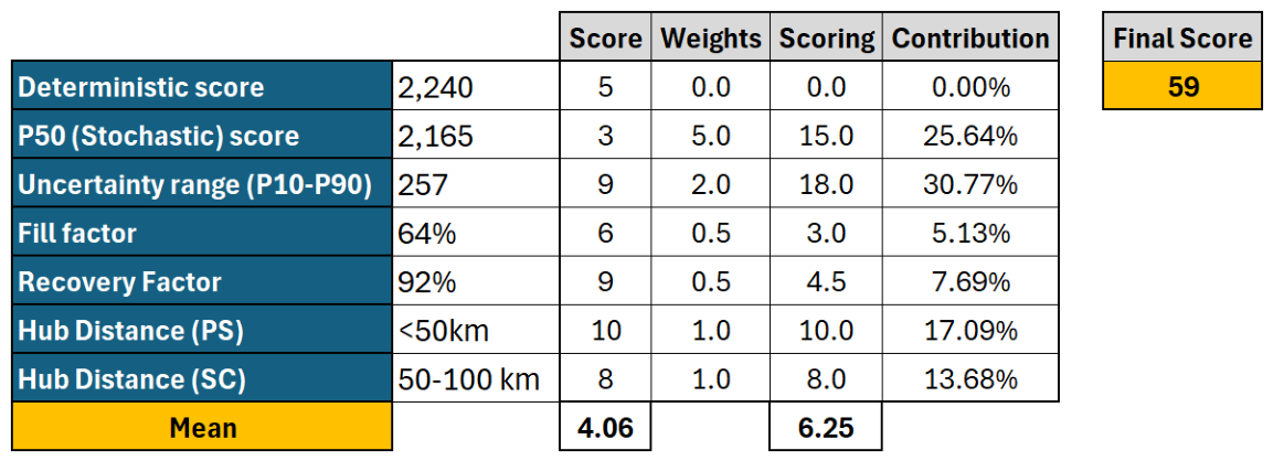
5.2.2. Astakos Area
Data obtained from legacy hydrocarbon-exploration data, including seismic profiles, structural interpretations and the Astakos-1 well, indicate the presence of an extensive evaporitic sequence. The well penetrated approximately 2,288 m of evaporites, with halite content of about 60% below 1,500 m and values increasing locally to approximately 80% between 2,700 and 3,323 m [65,66]. For the common target interval adopted in the present assessment, the conservative value of 60% was therefore used, assigning Astakos to “Tolerable (≥60%)”. In contrast to Filiates, this classification is supported by direct well information, hence “High”.
For Tectonics, Astakos presents a similar setting to Filiates. The principal fault systems are interpreted to occur mainly along the margins of the targeted evaporite body rather than to penetrate the selected storage interval. The same “No faults” was therefore assigned. Furthermore, as for Filiates, the available information does not provide a dedicated high-resolution structural characterization of the proposed cavern area, and a “Medium” was consequently retained for this criterion.
As explained in Section 5.1, microbial activity is absent for the case-study application. For Astakos, the availability of direct well information confirming a halite-dominated, highly saline evaporitic sequence provides stronger indirect support for this assumption than at the other investigated sites. Therefore a “High” is assigned.
Astakos is closer to the Ionian islands were important earthquakes have been recorded (Kefalonia and Zakinthos), seismicity was treated as “1 to 5 Rt”, however to map the chance of a severe earthquake event in future, the criterion has been accompanied by “Medium” to map the chance of a 5 to 7 Rt event.
The Astakos configuration shown in Figure 19 resulted in a value. The criterion-level contribution profile, presented in Figure 20a, is dominated by Salt Structure, Lithology, and Depth, which account for 24.71%, 21.18%, and 19.61% respectively. The resulting cumulative probability distribution for Astakos is shown in Figure 19b, resulting in , , and , and .
For the specified storage requirement, Astakos yields a and a . Moreover, in regard to Astakos infrastructure configuration, the evaluated area lies close to the port of Astakos, approximately 20 km from the proposed EastMed pipeline corridor and approximately 30 km from the city of Agrinio. Therefore, both and relationships fall within the “<50 km” distance category.
As shown in Figure 21 for Astakos, is mapped to a Score of 9, whereas is mapped to 8 (second lowest uncertainty value). Similarly, and are converted to Scores of 5 and 7, respectively, while the and are converted both to Score 10. Finally, the assessment yields to a = 87.
5.2.3. Zante Island
The Zante area assessment relies mainly on four seismic profiles—three offshore and one onshore—together with published geological and seismotectonic interpretations of the area [67,68,69,70]. Unlike Astakos, no exploratory well has penetrated the deeper part of the targeted evaporitic structure. Consequently, several of the Zante-specific assignments rely mostly on seismic interpretation and regional geological evidence.
The evaporites exposed at Skopos Mountain are strongly affected by near-surface alteration and dissolution and are described as gypsum- and anhydrite-rich [63,71]. These surface characteristics are not considered representative of the deeper storage interval, while direct information on the halite content at depth is unavailable. Based on the general descriptions of a halite-rich evaporitic sequence, a halite content of approximately 70% was adopted for the case-study application, corresponding to “Fair (≥70%)”, accompanied by a “Medium” since the category was inferred rather than been supported by direct deep-well measurements.
Tectonics represents a clearer departure from Filiates and Astakos. The seismic profiles available for Zante cross the salt structure directly and provide a more explicit representation of the local fault framework. The interpreted faults occur around the targeted evaporitic body without being considered to penetrate the selected storage interval; the criterion was therefore assigned to “Faults around the evaporite but not penetrate”. Owing to the more direct seismic evidence available for this site, a “High” level was assigned to this interpretation.
Although the interpreted evaporitic sequence encompasses the common target interval, its depth is derived from time-to-depth conversion of seismic data using a generalized velocity model. In the absence of a deep well for local calibration, greater uncertainty remains in the absolute depth and geometry of the target interval. The “500 < Depth < 2000” category is therefore retained, but with a “Low”. Note that this combination penalizes the site but it still screens at as acceptable (see Appendix A4).
For Microbial Presence, the common microbe’s absence assumption is maintained and the lack of direct microbiological information leads to a “Medium”.
Zante area lies really close Kefalonia and Zakinthos, therefore inheriting chances of severe seismicity events. To map this situation, the seismicity category was downgraded to “5 to 7 Rt”, with a high confidence stated by “High”.
The Zante configuration produces a , Figure 22. In contrast to Astakos and Filiates, the criterion-level contribution profile is more strongly concentrated in Salt Structure and Tectonics, which account for approximately 32.98% and 25.13% of the deterministic score, respectively, followed by Lithology at approximately 18.85%, presented in Figure 23a. Followingly, the stochastic assessment, Figure 23b, produces , , and , corresponding to .
For the specified storage requirement, Zante yields a and a . From an infrastructure perspective, Zante is located approximately 8 km from both the regional airport and the port of Zante, providing close access to local transport and consumption infrastructure. The proposed EastMed pipeline corridor is farther away, at approximately 93 km. These distances are subsequently represented through the and indicators used in the final-ranking assessment.
As shown in Figure 24, is mapped to a Score of 1 (lowest in the storage sites list) and is also mapped to a Score of 1 (maximum uncertainty range). Similarly, and are converted to Scores of 6 and 8, respectively, while the and are converted to Score 10 and 8 respectively. Finally, the assessment yields to a = 32.
5.3. Discussion
The Static input data for the three assessed sites are provided in Table A7 of the Appendix. Considering, the main deterministic, stochastic, engineering, and final-ranking results obtained for the three candidate sites are summarized in Table 1.
The comparative assessment of the three candidate areas demonstrates that their relative ranking at the present stage is controlled by the geological conditions assigned to each Static criterion further supported by the confidence level associated with the available information. This distinction is particularly important at an early screening stage, where the amount and quality of subsurface information may differ substantially among candidate sites. Accordingly, the Static score should not be interpreted solely as an indication of geological quality, but as the combined outcome of criterion suitability, confidence, and the assigned importance weights.
Lithology provides the clearest example. Filiates and Zante are represented by the more favorable “Fair (≥70%)” category, whereas Astakos is assigned to a slightly lower category “Tolerable (≥60%)”. However, the Filiates and Zante assignments are based predominantly on geological interpretation and indirect information and are therefore associated with Medium Confidence. In contrast, the halite content at Astakos is constrained by the Astakos-1 exploratory well and is assigned High Confidence. As a result, despite its less favorable Lithology category, Astakos obtains a larger criterion-level contribution. This effect is particularly significant because Lithology exhibits highest importance weight in the adopted configuration, . Numerically, the resulting weighted Lithology contribution in is 540 for Astakos, compared with 360 for both Filiates and Zante. The additional geological information available at Astakos therefore more than compensates, within the present scoring framework, for its lower assigned halite-content category.
Tectonics presents the opposite behavior to Lithology. Filiates and Astakos are both assigned to the “No faults” category with Medium Confidence. This does not imply an absence of regional faulting; rather, the available interpretation indicates that the candidate storage areas can be positioned within parts of the evaporitic bodies where faults are not interpreted to penetrate the selected storage interval. Zante is assigned to the less favorable “Faults around the evaporite but not penetrate” category, but the seismic profiles cross the structure more directly and provide a stronger basis for the local structural interpretation. High confidence level is therefore attributed to Zante, results in a larger Tectonics contribution. The corresponding Importance weight, , is lower than that assigned to Lithology, hence it does not dominate the overall Static assessment.
Depth constitutes the strongest unfavorable distinction for Zante. Although the same “500 < Depth < 2000” category is adopted for all three areas, the depth interpretation for Zante is derived from seismic information requiring time-to-depth conversion and lacks direct deep-well calibration, hence Low Confidence is assigned, whereas Filiates and Astakos retain High Confidence for the same category. In such case, the complete lack of confidence significantly reduces the contribution of the specific criterion for Zante, thus indirectly favoring other sites.
Field Status is also horizontally identical among the three sites and therefore has no effect on their present relative ranking. This criterion has a comparatively high Importance weight, , and could become influential if one candidate advances to a different development stage. For example, under the current High Confidence assignment, moving from “Not working yet” to “Under development” would increase its weighted contribution from 80 to 400, while a transition to “Currently working” would increase it to 800.
For Microbial Presence, distinction again arises through the information confidence level. Astakos is assigned High Confidence because of direct well information which provides stronger evidence for the halite-dominated and highly saline character of the evaporitic sequence. On the other hand, the Medium Confidence retained for Filiates and Zante allows Astakos to receive a larger contribution from this criterion. Its low Importance weight of limits should not be interpreted as rendering Microbial Presence uncritical. Under the adopted screening framework, a future assignment to “Present” corresponds to a Rejected suitability class and would activate the hard-screening rule rather than merely reduce the weighted Static score.
Seismicity is represented through site-specific category and Confidence assignments. Filiates is assigned to the “1 to 5 Rt” category with High Confidence, Astakos to the same category with Medium Confidence, and Zante to the “5 to 7 Rt” category with High Confidence. Based on the criterion scores defined in Table A2, the resulting weighted Seismicity contributions are 140 for Filiates, 70 for Astakos, and 80 for Zante, clearly rendering Filiates as the leader in this aspect. Nevertheless, Seismicity has the lowest adopted Importance weight, , hence these differences exert only a limited influence on the overall Static ranking. Again, improved site-specific characterization could alter the corresponding category and/or Confidence assignment in a subsequent evaluation.
Taken together, the deterministic results yield for Astakos, 2,240 for Filiates, and 1,910 for Zante. Astakos therefore ranks first in the deterministic Static assessment whereas Zante is ranked last with a remarkably low score.
For the final-ranking exercise, the stochastic Static assessment was selected instead of the deterministic Static score. This choice does not alter the ordering established by the deterministic assessment since follows similar distribution among the three sites: Astakos remains first with , followed by Filiates with and Zante with . The principal difference is that the stochastic formulation also offers the uncertainty associated with the Confidence distributions through . Filiates exhibits the narrowest uncertainty range, 257, followed closely by Astakos at 282, while Zante presents the widest range, 416. Although Astakos benefits from the availability of exploratory-well information, its uncertainty range is slightly wider than that of Filiates under the specific probability distributions and parameters adopted in the present stochastic configuration.
These results are directly illustrated in Figure 25, where the cumulative probability distributions of the three sites are presented together. The Astakos distribution is shifted to the right providing a clear graphical representation of its advantage in under the current level of data availability. Filiates occupies an intermediate position but exhibits the narrowest stochastic range, whereas Zante shows a lower central Static score and the broadest uncertainty interval. The higher of Astakos therefore provides the main geological basis for its advantage when the assessment proceeds from the Static stage to the final-ranking calculation.
The engineering indicators provide a different perspective. Filiates achieves the most favorable performance, with and , compared with 53% and 69% for Astakos and 60% and 82% for Zante, respectively. Therefore, Astakos, although favored by the Static assessment, is not the strongest candidate from the perspective of storage utilization and recoverability. Under the weighting configuration adopted for this early-stage assessment, however, the stochastic Static component receives substantially greater emphasis than the engineering indicators, whose Importance values are currently 0.5 each.
As the project progresses and the geological characterization becomes more mature, the Importance assigned to , , and other project-oriented indicators could reasonably increase. In such a configuration, the strong operational performance of Filiates would increase its contribution to . This does not imply that Filiates would necessarily overtake Astakos; rather, its relative ranking would improve depending on the specific Importance values adopted for the more mature decision stage. The same reasoning applies to the Hub Distance indicators. Their present values reflect the infrastructure and market assumptions adopted for the current scenario, but producer and consumer locations, pipeline development, port utilization, and hydrogen-market requirements can evolve. These indicators should therefore be reassessed whenever a specific operational scenario is defined.
Under the present early-stage configuration and available information, the resulting Final Scores are 87 for Astakos, 59 for Filiates, and 32 for Zante. Astakos consequently ranks first, primarily because the stronger evidence supporting its Static characterization. Filiates, despite providing the strongest Fill Factor and Recovery Factor, remains second because these operational indicators have limited influence under the current weighting strategy. Zante ranks third, mainly because the uncertainty associated with its subsurface characterization, particularly Depth, limits its Static assessment.
The resulting ranking should therefore be interpreted as a snapshot of the decision problem under the present stage of knowledge rather than as a permanent ordering of the three geological areas. New exploratory wells, higher-resolution seismic interpretation, dedicated stress measurements, microbiological characterization, or changes in the project and infrastructure scenario can modify the selected categories, Confidence levels, stochastic distributions, and ranking weights and may consequently alter both the individual scores and the final site ordering. This represents an important feature of the proposed DMT: as the available evidence matures, the assessment can be updated without changing the underlying methodological framework.
Future development of the DMT should focus on the development and validation of weighting configurations tailored to different stages of storage-project maturity, allowing the relative importance of geological, uncertainty-related, engineering, and Operator-defined factors to evolve as additional project information becomes available. The stochastic framework could also be extended beyond Confidence uncertainty by introducing probability distributions directly for selected geological and engineering inputs where sufficient data are available. Further work should examine the sensitivity of the ranking to the adopted category boundaries, scoring functions, and exclusion thresholds and support their refinement as additional field and operational evidence becomes available.
At more advanced stages, the screening workflow could be coupled with higher-fidelity cavern-scale geomechanical and dynamic models to evaluate cyclic operation, cavern deformation, well performance, and injection-withdrawal constraints. Finally, the incorporation of a dedicated techno-economic module could extend the current engineering-oriented assessment to include development and operating costs, cushion-gas requirements, compression, transportation, and other economic factors relevant to project-specific decision-making.
6. Conclusions
The development of large-scale UHS requires a systematic approach capable of integrating geological suitability with the uncertainty of available subsurface information, cavern and operating characteristics, and project-specific requirements. This study presents a holistic Decision-Making Tool (DMT) for the preliminary screening and comparative ranking of potential hydrogen storage sites in salt formations. The methodology combines deterministic assessment of eight geological criteria with a stochastic treatment of their associated uncertainties, engineering calculations of storage performance, and operator-defined requirements. The resulting framework therefore moves beyond a purely geological screening exercise and provides a structured link between subsurface characteristics and the conditions under which a storage project is intended to operate.
A particular strength of the proposed approach is its ability to explicitly retain the uncertainty associated with the available geological information. Rather than treating the input data as equally reliable and deterministic, the methodology allows confidence levels to be assigned to the individual criteria and propagates these uncertainties through a Monte Carlo procedure. This provides not only a single site-suitability score but also an indication of the robustness of that assessment. The weighting of the different ranking components can subsequently be adjusted according to the objective and maturity of the screening exercise, while the same weighting configuration can be consistently applied to all candidate sites being compared.
The application to Filiates, Astakos and Zante in western Greece demonstrates the value of combining these different information sources. Although all three investigated areas present potentially suitable evaporitic formations, their relative performance differs when geological suitability, confidence in the available information, storage performance and proximity to relevant hydrogen infrastructure are considered simultaneously. Under the ranking configuration adopted in this study, Astakos obtained the highest final score, supported by its geological suitability, larger overall capacity and favourable location. Filiates, however, exhibited the highest confidence in the available geological assessment and the highest fill level for the common storage target, illustrating that the site with the highest overall ranking is not necessarily the site that performs best with respect to every individual criterion.
The results also demonstrate that the proposed DMT should be regarded as a decision-support framework rather than a replacement for detailed site characterization and engineering studies. Its principal value lies at the preliminary screening and comparative-ranking stage, where decisions must be made despite incomplete and uncertain information. The Excel implementation makes the methodology transparent, reproducible and traceable, while allowing the ranking strategy to be adapted as the objectives of a project evolve or as additional sites and improved data become available. The methodology can therefore provide a common framework within which geological knowledge, uncertainty and engineering requirements can be progressively incorporated as a project advances toward more detailed evaluation.
Finally, the study demonstrates that site selection for underground hydrogen storage is inherently scenario-dependent. There is no universally optimal site independent of the objectives and constraints imposed on the storage project. The ability to modify the relative importance of geological suitability, storage utilization, recoverability and infrastructure-related criteria allows the proposed methodology to accommodate different stages and objectives of site evaluation without changing the underlying calculations. As the number of candidate sites increases and the quality of the available geological and operational data improves, further calibration of the ranking weights and expansion of the database will strengthen the comparative capability of the tool and its applicability to broader hydrogen-storage site-selection exercises.
Author Contributions
Conceptualization, D.D., P.T., S.B. and V.G.; methodology, D.D. and P.T.; software, D.D.; validation, P.T., S.B. and E.M.K.; formal analysis, D.D. and V.G.; investigation, D.D and P.T.; data curation, P.T.; writing—original draft preparation, D.D. and E.M.K.; writing—review and editing, V.G., E.S. and S.B.; supervision, V.G.; All authors have read and agreed to the published version of the manuscript.
Funding
We gratefully acknowledge the support provided by TWINN2SET project, under the grant number 101079246 funded by Horizon Europe.
Nomenclature
| Category of criterion | |
| Set of available categories of criterion | |
| Numerical score of criterion | |
| Confidence category of criterion | |
| Set of available confidence categories of criterion | |
| Numerical value of criterion confidence level | |
| Suitability category of criterion | |
| Set of available suitability categories of criterion | |
| Static criterion total score | |
| Importance weight of criterion in the static score of a site | |
| Static score of a site | |
| Importance weight value of factor in the site score | |
| Difference between the 90th and 10th percentiles of Static score of a site | |
| Total site score | |
| Nominal site mass capacity | |
| Fill factor of a site’s cluster of caverns | |
| Fill factor of a site | |
| Recovery factor of a site | |
| Bulk cavern volume | |
| Leaching ratio | |
| Gas compressibility factor | |
| Cavern temperature | |
| Hydrogen molar mass | |
| Universal gas constant | |
| Storage capacity of cavern | |
| Hydrogen mass remaining for allocation during the cluster-filling procedure | |
| Storage capacity of the considered cavern cluster | |
| Maximum allowable operating pressure of cluster | |
| Minimum allowable operating pressure of cluster | |
| Hydrogen mass stored in cluster at the maximum allowable operating pressure | |
| Cushion-gas mass in cluster at the minimum allowable operating pressure | |
| Recoverable hydrogen mass of cluster | |
| Producer-to-site distance score | |
| Site-to-consumer distance score | |
| Gating term applied to the final site score |
Appendix A

Table A1.
Parameters required for the probability distributions supported in the stochastic confidence assessment, where μ: mean; Mo: mode; σ: standard deviation; Min and Max: lower and upper admissible bounds.
Table A1.
Parameters required for the probability distributions supported in the stochastic confidence assessment, where μ: mean; Mo: mode; σ: standard deviation; Min and Max: lower and upper admissible bounds.
| Normal | Lognormal | Triangular | Uniform | |
|---|---|---|---|---|
| μ | √ | √ | ||
| Mode | √ | |||
| σ | √ | √ | ||
| Min | √ | √ | ||
| Max | √ | √ |
Table A2, Table A3, Table A5 and Table A6 proposed values should be considered indicative rather than fixed, as they may be reconsidered and adjusted according to engineering judgment and expert knowledge, reflecting the modularity of the proposed methodology.
Table A2.
Numerical scoring & weighting framework for the site criteria.
| Criterion | Importance weight | Category | Score | Suitability class |
|---|---|---|---|---|
| Lithology | 9 | Pure | 9 | High |
| Fair | 8 | Medium | ||
| Tolerable | 6 | Low | ||
| Rejected | 1 | Rejected | ||
| Salt structure | 7 | Salt dome | 9 | High |
| Thick bedded salt | 8 | Medium | ||
| Breccia salt | 3 | Rejected | ||
| Thin bedded or layered | 1 | Rejected | ||
| Tectonics | 6 | No faults | 10 | High |
| Faults around the evaporite but not penetrate | 8 | Medium | ||
| Some faults penetrate locally the evaporite | 3 | Low | ||
| Severe fracturing | 1 | Rejected | ||
| Depth | 5 | < 500 | 5 | Medium |
| 500 < Depth < 2000 | 10 | High | ||
| > 2000 | 1 | Low | ||
| Field status | 8 | Currently working | 10 | High |
| Under development | 5 | Medium | ||
| Not working yet | 1 | Low | ||
| Microbial presence | 4 | Absent | 10 | High |
| Present | 1 | Rejected | ||
| Stress state | 3 | Isotropic | 10 | High |
| Anisotropic | 1 | Low | ||
| Seismicity | 2 | 0 Rt | 10 | High |
| 1 to 5 Rt | 7 | Medium | ||
| 5 to 7 Rt | 4 | Low | ||
| > 7 Rt | 1 | Rejected |
Table A3.
Numerical values assigned to data confidence.
| Data confidence | Score | Inclusion mapping |
|---|---|---|
| High | 10 | High |
| Medium | 5 | Medium |
| Low | 1 | Low |
Table A4.
Inclusion–exclusion logic applied to the criterion-level suitability assessment. Symbols denote: √, satisfying suitability condition and criterion inclusion; ×, non-satisfying suitability condition resulting in a zero-criterion score and immediate site exclusion; √×, limiting satisfying condition, located on the diagonal boundary between inclusion and exclusion; the criterion remains included, but represents the minimum admissible combination of suitability and confidence.
Table A4.
Inclusion–exclusion logic applied to the criterion-level suitability assessment. Symbols denote: √, satisfying suitability condition and criterion inclusion; ×, non-satisfying suitability condition resulting in a zero-criterion score and immediate site exclusion; √×, limiting satisfying condition, located on the diagonal boundary between inclusion and exclusion; the criterion remains included, but represents the minimum admissible combination of suitability and confidence.
| Suitability | |||||
|---|---|---|---|---|---|
| High | Medium | Low | Rejected | ||
| Confidence | High | √ | √ | √x | x |
| Medium | √ | √x | x | x | |
| Low | √x | x | x | x | |
Table A5.
Producer-to-site & Site-to-consumer distance scoring.
| Producer to site | Score | Site to consumer | Score |
|---|---|---|---|
| Port/ Pipelines | 9 | Port/ Pipelines/ Airport | 9 |
| < 50 km | 10 | < 50 km | 10 |
| 50 – 100 km | 8 | 50 – 100 km | 8 |
| 100 – 250 km | 6 | 100 – 250 km | 6 |
| 250 – 500 km | 4 | 250 – 500 km | 4 |
| > 500 km | 1 | > 500 km | 1 |
Table A6.
Final ranking components importance values.
| Ranking components | Importance value |
|---|---|
| Deterministic static score | 0 |
| Stochastic static score | 5.0 |
| Uncertainty | 2.0 |
| Fill Factor | 0.5 |
| Recovery Factor | 0.5 |
| Hub Distance - Producer to site | 1.0 |
| Hub Distance - Site to consumer | 1.0 |
Table A7.
Static data per site.
| Case studies regions |
Lithology | Salt Structure |
Tectonics | Depth | Field Status | Microbes Presence | Stress State | Seismicity |
|---|---|---|---|---|---|---|---|---|
| Filiates | Fair (>= 70) | Salt dome | No faults | 500 < D < 2000 | Not working yet | Absent | Anisotropic | 1 to 5 Rt |
| Medium | High | Medium | High | High | Medium | High | High | |
| Astakos | Tolerable (>= 60) | Salt dome | No faults | 500 < D < 2000 | Not working yet | Absent | Anisotropic | 1 to 5 Rt |
| High | High | Medium | High | High | High | High | Medium | |
| Zante | Fair (>= 70) | Salt dome | Faults around the evaporite but not penetrate | 500 < D < 2000 | Not working yet | Absent | Anisotropic | 5 to 7 Rt |
| Medium | High | High | Low | High | Medium | High | High |
References
- Muhammed, N. S.; Haq, B.; Al Shehri, D.; Al-Ahmed, A.; Rahman, M. M.; Zaman, E. A Review on Underground Hydrogen Storage: Insight into Geological Sites, Influencing Factors and Future Outlook. Energy Rep. 2022, 8, 461–499. [Google Scholar] [CrossRef]
- Zivar, D.; Kumar, S.; Foroozesh, J. Underground Hydrogen Storage: A Comprehensive Review. Int. J. Hydrogen Energy 2021, 46, 23436–23462. [Google Scholar] [CrossRef]
- Tackie-Otoo, B. N.; Haq, B. A Comprehensive Review on Geo-Storage of H2 in Salt Caverns: Prospect and Research Advances. Fuel 2024, 356, 129609. [Google Scholar] [CrossRef]
- Warren, J. K. Salt Usually Seals, but Sometimes Leaks: Implications for Mine and Cavern Stabilities in the Short and Long Term. Earth-Sci. Rev. 2017, 165, 302–341. [Google Scholar] [CrossRef]
- Minougou, J. D.; Gholami, R.; Andersen, P. Underground Hydrogen Storage in Caverns: Challenges of Impure Salt Structures. Earth-Sci. Rev. 2023, 247, 104599. [Google Scholar] [CrossRef]
- Abreu, J. F.; Costa, A. M.; Costa, P. V. M.; Miranda, A. C. O.; Zheng, Z.; Wang, P.; Goulart, M. B. R.; Bergsten, A.; Ebecken, N. F. F.; Bittencourt, C. H.; Assi, G.; Meneghini, J. R.; Nishimoto, K. Large-Scale Storage of Hydrogen in Salt Caverns for Carbon Footprint Reduction. Int. J. Hydrogen Energy 2023, 48, 14348–14362. [Google Scholar] [CrossRef]
- Zhang, N.; Li, J.; Xu, W.; Naumov, D.; Zill, F.; Chen, Y.; Nagel, T. Mind the Sump: Solution Mining-Based Reconstruction of Sediment-Filled Regions for Improved Stability Modeling of Salt Caverns. Tunn. Undergr. Space Technol. 2026, 170, 107352. [Google Scholar] [CrossRef]
- Şan, S.; Karakılçık, H.; Karakılçık, M.; Erden, M.; Atiz, A. Investigation of Cushion Gas/Working Gas Ratios of Underground Salt Caverns for Hydrogen Storage. In Emerging Trends in Energy Storage Systems and Industrial Applications; Elsevier, 2023; pp. 67–78. [Google Scholar] [CrossRef]
- Allsop, C.; Yfantis, G.; Passaris, E.; Edlmann, K. Utilizing Publicly Available Datasets for Identifying Offshore Salt Strata and Developing Salt Caverns for Hydrogen Storage. Geol. Soc. Spec. Publ. 2023, 528, 139–169. [Google Scholar] [CrossRef]
- Jannel, H.; Torquet, M. HYSTORIES: Conceptual Design of Salt Cavern and Porous Media Underground Storage Site; 2022. [Google Scholar]
- Heinemann, N.; Alcalde, J.; Miocic, J. M.; Hangx, S. J. T.; Kallmeyer, J.; Ostertag-Henning, C.; Hassanpouryouzband, A.; Thaysen, E. M.; Strobel, G. J.; Schmidt-Hattenberger, C.; Edlmann, K.; Wilkinson, M.; Bentham, M.; Haszeldine, R. S.; Carbonell, R.; Rudloff, A. Enabling Large-Scale Hydrogen Storage in Porous Media—The Scientific Challenges. Energy Environ. Sci. 2021, 14, 853–864. [Google Scholar] [CrossRef]
- Thaysen, E. M.; McMahon, S.; Strobel, G. J.; Butler, I. B.; Ngwenya, B. T.; Heinemann, N.; Wilkinson, M.; Hassanpouryouzband, A.; McDermott, C. I.; Edlmann, K. Estimating Microbial Growth and Hydrogen Consumption in Hydrogen Storage in Porous Media. Renew. Sustain. Energy Rev. 2021, 151, 111481. [Google Scholar] [CrossRef]
- Montazeri, M.; Salmachi, A.; Haghighi, M.; Hosseini, T. Large-Scale Hydrogen Storage: Surface and Subsurface Challenges. ChemBioEng Rev. 2026, 13. [Google Scholar] [CrossRef]
- Seyed Ghafouri, S. M. H.; Younes, J.; Grasselli, G. Geomechanics of Geological Storage of Hydrogen: Knowledge Gaps and Future Directions. Renew. Sustain. Energy Rev. 2026. [Google Scholar] [CrossRef]
- Wang, T.; Yang, C.; Ma, H.; Daemen, J. J. K.; Wu, H. Safety Evaluation of Gas Storage Caverns Located Close to a Tectonic Fault. J. Nat. Gas Sci. Eng. 2015, 23, 281–293. [Google Scholar] [CrossRef]
- Lu, L.; Shi, Y.; Wang, M.; Ye, M.; Zuo, C.; Shun, X. Seismic Performance of Salt Cavern Gas Storage Subjected to Moderate Earthquake Loads in Compressed CO2 Energy Storage Scenario. Energy Rep. 2025, 13, 2366–2383. [Google Scholar] [CrossRef]
- Lin, N.; Patonia, A.; Shuster, M.; Lambert, M.; Zhang, T. Natural Hydrogen Techno-Economics and Valuation. Appl. Energy 2026, 408. [Google Scholar] [CrossRef]
- Matos, C. R.; Carneiro, J. F.; Silva, P. P. Overview of Large-Scale Underground Energy Storage Technologies for Integration of Renewable Energies and Criteria for Reservoir Identification. J. Energy Storage 2019, 21, 241–258. [Google Scholar] [CrossRef]
- Nemati, B.; Mapar, M.; Davarazar, P.; Zandi, S.; Davarazar, M.; Jahanianfard, D.; Mohammadi, M. A Sustainable Approach for Site Selection of Underground Hydrogen Storage Facilities Using Fuzzy-Delphi Methodology. J. Settl. Spat. Plan. 2020, 2020, 5–16. [Google Scholar] [CrossRef]
- Huang, L.; Fang, Y.; Hou, Z.; Xie, Y.; Wu, L.; Luo, J.; Wang, Q.; Guo, Y.; Sun, W. A Preliminary Site Selection System for Underground Hydrogen Storage in Salt Caverns and Its Application in Pingdingshan, China. Deep Undergr. Sci. Eng. 2024, 3, 117–128. [Google Scholar] [CrossRef]
- Ruiz Maraggi, L. M.; Moscardelli, L. G. Hydrogen Storage Potential of Salt Domes in the Gulf Coast of the United States. J. Energy Storage 2024, 82. [Google Scholar] [CrossRef]
- Malki, M. L.; Chen, B.; Mao, S.; Chen, F.; Mehana, M. OPERATE–H2: A Tool for Optimizing Underground Hydrogen Storage. J. Energy Storage 2024, 90. [Google Scholar] [CrossRef]
- Lankof, L.; Luboń, K.; Le Gallo, Y.; Tarkowski, R. The Ranking of Geological Structures in Deep Aquifers of the Polish Lowlands for Underground Hydrogen Storage. Int. J. Hydrogen Energy 2024, 62, 1089–1102. [Google Scholar] [CrossRef]
- Harati, S.; Rezaei Gomari, S.; Ramegowda, M.; Pak, T. Multi-Criteria Site Selection Workflow for Geological Storage of Hydrogen in Depleted Gas Fields: A Case for the UK. Int. J. Hydrogen Energy 2024, 51, 143–157. [Google Scholar] [CrossRef]
- Borghini, L.; Corradetti, A.; Del Ben, A.; Franceschi, M.; Bonini, L. Underground Hydrogen Storage Suitability Index: A Geological Tool for Evaluating and Ranking Storage Sites. Int. J. Hydrogen Energy 2025, 149. [Google Scholar] [CrossRef]
- Blancone, D.; Ruiz Maraggi, L. M.; Cardozo, N.; Moscardelli, L.; Escalona, A. Assessing Hydrogen Storage Potential in Zechstein Salt Caverns of the Norwegian North Sea. J. Energy Storage 2025, 128. [Google Scholar] [CrossRef]
- Anzelmo, G.; Cella, G. M.; Magistroni, C.; Da Pra, A.; Iacopini, D. Methodological Workflow for Screening and Ranking Salt Caverns for Underground Hydrogen Storage: The CRS Approach; 2026. [Google Scholar] [CrossRef]
- Trimi, P.-M.; Bellas, S.; Vakalas, I.; Gholami, R.; Gaganis, V.; Gontikaki, E.; Stamatakis, E.; Yentekakis, I. A Review of Caprock Integrity in Underground Hydrogen Storage Sites: Implication of Wettability, Interfacial Tension, and Diffusion. Hydrogen 2025, 6, 91. [Google Scholar] [CrossRef]
- Garvey, C.; Armitage, T.; Todd, J.; Noone, M.; Seakins, J.; Edlmann, K. Revising the Theoretical Storage Potential of Hydrogen in UK Salt Caverns: A Multi-Criteria Assessment of the East Coast of England. Geoenergy 2026, 4. [Google Scholar] [CrossRef]
- Snow, J. H.; Doré, A. G.; Dorn-Lopez, D. W. Risk Analysis and Full-Cycle Probabilistic Modelling of Prospects: A Prototype System Developed for the Norwegian Shelf. Nor. Pet. Soc. Spec. Publ. 1996, 6, 153–165. [Google Scholar] [CrossRef]
- Kanakaki, E. M.; Gaganis, V. Automated Equations of State Tuning Workflow Using Global Optimization and Physical Constraints. Liquids 2024, 4, 261–277. [Google Scholar] [CrossRef]
- Neal, J. T.; Magorian Amherst, T. R.; York, N.; Thoms, R. L.; Autin, W. J.; Mcculloh, R. P.; Denzler, S.; Byrne, K. O. Anomalous Zones in Gulf Coast Salt Domes with Special Reference to Big Hill, TX, and Weeks Island, LA; 1993. [Google Scholar] [CrossRef]
- Duffy, O.; Hudec, M.; Peel, F.; Apps, G.; Bump, A.; Moscardelli, L.; Dooley, T.; Bhattacharya, S.; Wisian, K.; Shuster, M. The Role of Salt Tectonics in the Energy Transition: An Overview and Future Challenges. Tektonika 2023, 1. [Google Scholar] [CrossRef]
- Michalski, J.; Bünger, U.; Crotogino, F.; Donadei, S.; Schneider, G. S.; Pregger, T.; Cao, K. K.; Heide, D. Hydrogen Generation by Electrolysis and Storage in Salt Caverns: Potentials, Economics and Systems Aspects with Regard to the German Energy Transition. Int. J. Hydrogen Energy 2017, 42, 13427–13443. [Google Scholar] [CrossRef]
- Cyran, K. The Influence of Impurities and Fabrics on Mechanical Properties of Rock Salt for Underground Storage in Salt Caverns – a Review. Arch. Min. Sci. 2021, 155–179. [Google Scholar] [CrossRef]
- Bruno, M. S.; Dusseault, M. B. Geomechanical Analysis of Pressure Limits for Thin Bedded Salt Caverns; 2002. [Google Scholar] [CrossRef]
- Gillhaus, A.; Horvath, P. Compilation of Geological and Geotechnical Data of Worldwide Domal Salt Deposits in Domal Salt Cavern Fields; 2008. [Google Scholar]
- Deng, F.; Jiang, F.; Wan, J.; Ji, W.; Li, J. Analysis of the Deformation Characteristics of Surrounding Rock Due to Interlayers during Cyclic Injection-Production Period of Salt Cavern Hydrogen Storage. Fuel 2025, 385, 134115. [Google Scholar] [CrossRef]
- Li, J.; Shi, X.; Yang, C.; Li, Y.; Wang, T.; Ma, H.; Shi, H.; Li, J.; Liu, J. Repair of Irregularly Shaped Salt Cavern Gas Storage by Re-Leaching under Gas Blanket. J. Nat. Gas Sci. Eng. 2017, 45, 848–859. [Google Scholar] [CrossRef]
- Wang, X.; Xiong, Q.; Zhou, H.; Chen, J.; Xiao, M. Three-Dimensional (3D) Dynamic Finite Element Modeling of the Effects of a Geological Fault on the Seismic Response of Underground Caverns. Tunn. Undergr. Space Technol. 2020, 96. [Google Scholar] [CrossRef]
- Ardeshiri-Lajimi, S.; Yazdani, M.; Assadi Langroudi, A. Control of Fault Lay-out on Seismic Design of Large Underground Caverns. Tunn. Undergr. Space Technol. 2015, 50, 305–316. [Google Scholar] [CrossRef]
- Qian, X.; You, S.; Wang, R.; Yue, Y.; Liao, Q.; Dai, J.; Tian, S.; Liu, X. Underground Hydrogen Storage in Salt Cavern: A Review of Advantages, Challenges, and Prospects. Sustainability 2025, 17, 5900. [Google Scholar] [CrossRef]
- Caglayan, D. G.; Weber, N.; Heinrichs, H. U.; Linßen, J.; Robinius, M.; Kukla, P. A.; Stolten, D. Technical Potential of Salt Caverns for Hydrogen Storage in Europe. Int. J. Hydrogen Energy 2020, 45, 6793–6805. [Google Scholar] [CrossRef]
- Evans, D. J.; Holloway, S. A Review of Onshore UK Salt Deposits and Their Potential for Underground Gas Storage. Geol. Soc. Lond. Spec. Publ. 2009, 313, 39–80. [Google Scholar] [CrossRef]
- Plaat, H. Underground Gas Storage: Why and How. Geol. Soc. Lond. Spec. Publ. 2009, 313, 25–37. [Google Scholar] [CrossRef]
- Williams, J. D. O.; Williamson, J. P.; Parkes, D.; Evans, D. J.; Kirk, K. L.; Sunny, N.; Hough, E.; Vosper, H.; Akhurst, M. C. Does the United Kingdom Have Sufficient Geological Storage Capacity to Support a Hydrogen Economy? Estimating the Salt Cavern Storage Potential of Bedded Halite Formations. J. Energy Storage 2022, 53, 105109. [Google Scholar] [CrossRef]
- Zhao, K.; Liu, Y.; Li, Y.; Ma, H.; Hou, W.; Yu, C.; Liu, H.; Feng, C.; Yang, C. Feasibility Analysis of Salt Cavern Gas Storage in Extremely Deep Formation: A Case Study in China. J. Energy Storage 2022, 47. [Google Scholar] [CrossRef]
- Al Homoud, R.; Machado, M. V. B.; Daigle, H.; Ates, H. Critical Geochemical and Microbial Reactions in Underground Hydrogen Storage: Quantifying Hydrogen Loss and Evaluating CO2 as Cushion Gas. Hydrogen 2025, 6, 4. [Google Scholar] [CrossRef]
- Aftab, A.; Salgar Chaparro, S. J.; Ali, M.; Xie, Q.; Saeedi, A.; Keshavarz, A.; Sarmadivaleh, M. Microbial Risk Assessment and Mitigation for Underground Hydrogen Energy Storage in Salt Caverns: A Multidisciplinary Investigation. Renew. Sustain. Energy Rev. 2026, 238, 117003. [Google Scholar] [CrossRef]
- Dopffel, N.; Mayers, K.; Kedir, A.; An-Stepec, B. A.; Beeder, J.; Hoth, S. Exploring Microbiological Dynamics in a Salt Cavern for Potential Hydrogen Storage Use. Environ. Microbiol. Rep. 2025, 17, e70064. [Google Scholar] [CrossRef] [PubMed]
- Dopffel, N.; An-Stepec, B. A.; Bombach, P.; Wagner, M.; Passaris, E. Microbial Life in Salt Caverns and Their Influence on H2 Storage – Current Knowledge and Open Questions. Int. J. Hydrogen Energy 2024, 58, 1478–1485. [Google Scholar] [CrossRef]
- Hoedeman, G.; Urai, J. L.; Schmatz, J.; Klaver, J. Over-Pressured Salt Solution Mining Caverns and Leakage Mechanisms Phase 1: Micro-Scale Processes; 2019. [Google Scholar]
- Zijp, M. H. A. A.; Huijgen, M. A.; Wilpshaar, M.; Bouroullec, R.; Ter, J. H. Stringers in Salt as a Drilling Risk; 2018. [Google Scholar] [CrossRef]
- Kupfer, D. H.; Lock, B. E.; Schank, P. R. Anomalous Zones Within the Salt at Weeks Island, Louisiana. Gulf Coast Assoc. Geol. Soc. Trans. 1998, 48, 181–191. [Google Scholar]
- Minkley, W.; Knauth, M.; Fabig, T.; Farag, N. Stability and Integrity of Salt Caverns under Consideration of Hydromechanical Loading. In Mechanical Behaviour of Salt VIII; CRC Press, 2015. [Google Scholar] [CrossRef]
- Wang, T.; Yang, C.; Yan, X.; Li, Y.; Liu, W.; Liang, C.; Li, J. Dynamic Response of Underground Gas Storage Salt Cavern under Seismic Loads. Tunn. Undergr. Space Technol. 2014, 43, 241–252. [Google Scholar] [CrossRef]
- Golghanddashti, H.; Sayyafzadeh, M.; Bunch, M.; Binda, A.; Zeinijahromi, A. Toward Accurate Subsurface Simulation for Underground Hydrogen Storage: EOS Evaluation and Viscosity Model Optimization. Int. J. Hydrogen Energy 2026, 219, 154067. [Google Scholar] [CrossRef]
- Karakitsios, V. The Influence of Preexisting Structure and Halokinesis on Organic Matter Preservation and Thrust System Evolution in the Ionian Basin, Northwest Greece. Am. Assoc. Pet. Geol. Bull. 1995, 79. [Google Scholar] [CrossRef]
- Kamberis, E.; Kokinou, E.; Koci, F.; Lioni, K.; Alves, T. M.; Velaj, T. Triassic Evaporites and the Structural Architecture of the External Hellenides and Albanides (SE Europe): Controls on the Petroleum and Geoenergy Systems of Greece and Albania. Int. J. Earth Sci. 2022, 111, 789–821. [Google Scholar] [CrossRef]
- Soto, J. I.; Tranos, M. D.; Bega, Z.; Dooley, T. P.; Hernández, P.; Hudec, M. R.; Konstantopoulos, P. A.; Lula, E.; Nikolaou, K.; Pérez, R.; Pita, J. P.; Titos, J. A.; Tzimeas, C.; Herra Sánchez de Movellán, A. Contrasting Styles of Salt-Tectonic Processes in the Ionian Zone (Greece and Albania): Integrating Surface Geology, Subsurface Data, and Experimental Models. Tectonics 2024, 43. [Google Scholar] [CrossRef]
- NOA. Available online: https://www.gein.noa.gr/ypiresies-proionta/katalogoi-seismon/.
- Marnelis, F.; Roussos, N.; Rigakis, N.; Karakitsios, V. Structural Geology of the Western Greece’s Fold-and-Thrust Belt; November 2007. [Google Scholar]
- Nikolaou, K. Contribution to the Knowlwdge of the Neogene and the Geology of the Ionian Preapulian Zones in Relation with Petroleum Exploration Mainly in the Islands of Strophades, Zante and Kephallinia; National and Kapodistrian University of Athens: Athens, 1986. [Google Scholar]
- Perrier, R.; Koukouzas, K.; Bizon, G. Geological Map of Greece, Scale 1:50000, Filiates Sheet; Institute of Geology and Mineral Exploration (I.G.M.E.), 1967. [Google Scholar]
- B.P. The Geological Results of Petroleum Exploration in Western Greece; 1971. [Google Scholar]
- Psonis, K. Geological Map of Greece, Scale 1:50000, Astakos Sheet; Institute of Geology and Mineral Exploration (I.G.M.E.), 1989. [Google Scholar]
- Lazos, I.; Sboras, S.; Kokkalas, S.; Karastathis, V.; Xiroudakis, G.; Iordanidou, K.; Galanakis, D.; Pikridas, C.; Bellas, S.; Karamitros, I.; Mouzakiotis, E.; Kanellopoulos, C.; Bitharis, S.; Chatzipetros, A.; Pavlides, S. Seismotectonic Implications for the Peloponnese (SW Greece) Region Based on Geodetic Crustal Deformation Analysis. Tectonophysics 2026, 918, 230969. [Google Scholar] [CrossRef]
- Karakitsios, V.; Roveri, M.; Lugli, S.; Manzi, V.; Gennari, R.; Antonarakou, A.; Triantaphyllou, M.; Agiadi, K.; Kontakiotis, G.; Kafousia, N.; de Rafelis, M. A Record of the Messinian Salinity Crisis in the Eastern Ionian Tectonically Active Domain (Greece, Eastern Mediterranean). Basin Res. 2017, 29, 203–233. [Google Scholar] [CrossRef]
- Kokinou, E.; Kamberis, E.; Vafidis, A.; Monopolis, D.; Ananiadis, G.; Zelilidis, A. Deep Seismic Reflection Data from Offshore Western Greece: A New Crustal Model for the Ionian Sea. J. Pet. Geol. 2005, 28, 185–202. [Google Scholar] [CrossRef]
- Kokkalas, S.; Kamberis, E.; Xypolias, P.; Sotiropoulos, S.; Koukouvelas, I. Coexistence of Thin- and Thick-Skinned Tectonics in Zakynthos Area (Western Greece): Insights from Seismic Sections and Regional Seismicity. Tectonophysics 2013, 597–598, 73–84. [Google Scholar] [CrossRef]
- Perry, L. J.; Temple, P. G.; Dimopoulos, V. Geological Map of Greece, Scale 1:50000, Zakynthos Island Sheet; Institute of Geology and Mineral Exploration (I.G.M.E.), 1980. [Google Scholar]
- Press, W. H.; Teukolsky, S. A.; Vetterling, W. T.; Flannery, B. P. Numerical Recipes: The Art of Scientific Computing, 3rd ed.; Cambridge University Press: Cambridge, 2007. [Google Scholar]
- IGI Poseidon. EastMed–Poseidon Project. [CrossRef] [PubMed]
Figure 1.
The development process of salt caverns: from site selection to commissioning.
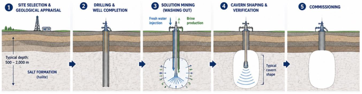
Figure 2.
The salt cavern operation: Injection (storage) and withdrawal (delivery) phases.
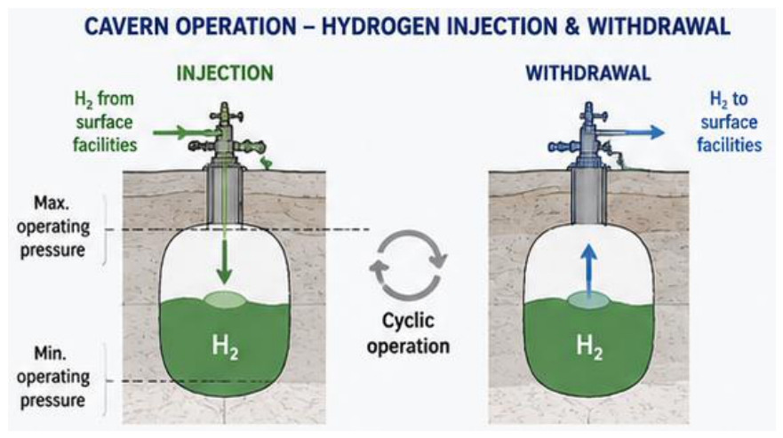
Figure 3.
Overview of the four data categories integrated in the Decision-Making Tool (DMT): Site Static data, Static-probabilistic data, Site Dynamic data, and Operator’s data, together with the principal criteria and inputs considered within each category.
Figure 3.
Overview of the four data categories integrated in the Decision-Making Tool (DMT): Site Static data, Static-probabilistic data, Site Dynamic data, and Operator’s data, together with the principal criteria and inputs considered within each category.
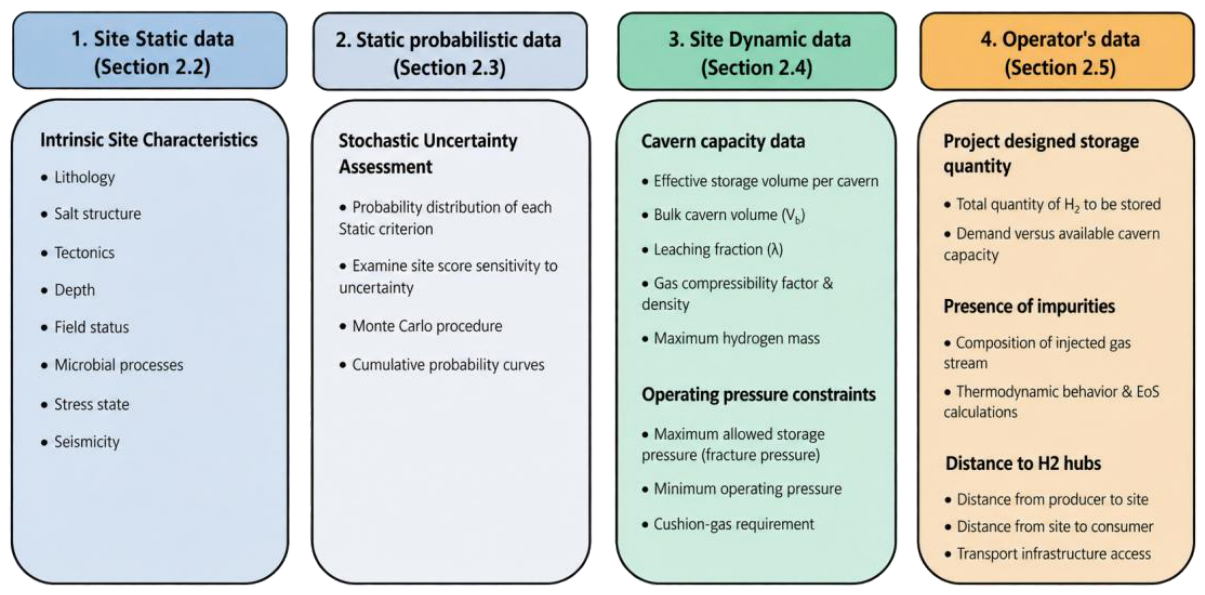
Figure 4.
Workflow to estimate the storage suitability score of a single site.
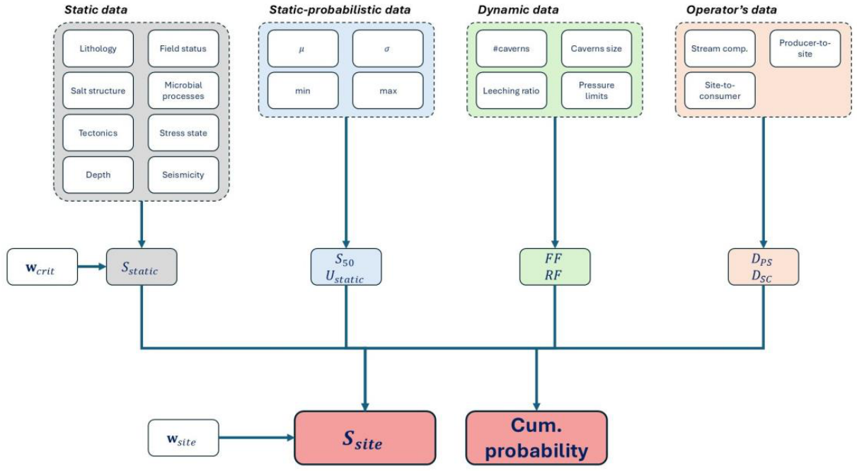
Figure 5.
Front-end implementation of the site identification and Static-data input block. The evaluated site is defined through the site name, unique site ID, and description fields, which provide traceability across stored assessments. The “Site criteria (deterministic)” Table presents the eight Static criteria and allows the user to specify, for each criterion, the selected Value/Category, , the corresponding Confidence level, , and the Importance weight, .
Figure 5.
Front-end implementation of the site identification and Static-data input block. The evaluated site is defined through the site name, unique site ID, and description fields, which provide traceability across stored assessments. The “Site criteria (deterministic)” Table presents the eight Static criteria and allows the user to specify, for each criterion, the selected Value/Category, , the corresponding Confidence level, , and the Importance weight, .
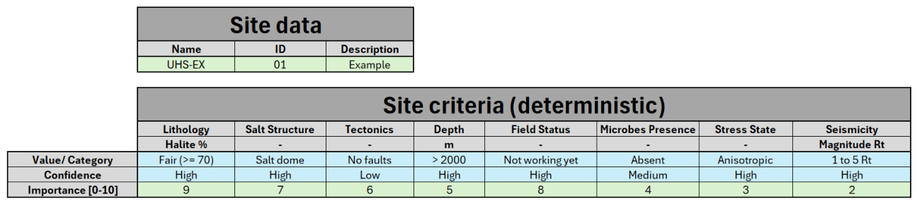
Figure 6.
Front-end implementation of the Static-probabilistic data input block. The “Site criteria (stochastic)” Table presents the eight Static criteria and allows the uncertainty associated with each criterion’s Confidence value, , to be defined. The deterministic Confidence value, , is used as the reference for the stochastic representation, while the Distribution row specifies the selected probability distribution. The subsequent rows contain the additional distribution-specific parameters required for the selected distribution, including and the min and max value, where applicable.
Figure 6.
Front-end implementation of the Static-probabilistic data input block. The “Site criteria (stochastic)” Table presents the eight Static criteria and allows the uncertainty associated with each criterion’s Confidence value, , to be defined. The deterministic Confidence value, , is used as the reference for the stochastic representation, while the Distribution row specifies the selected probability distribution. The subsequent rows contain the additional distribution-specific parameters required for the selected distribution, including and the min and max value, where applicable.
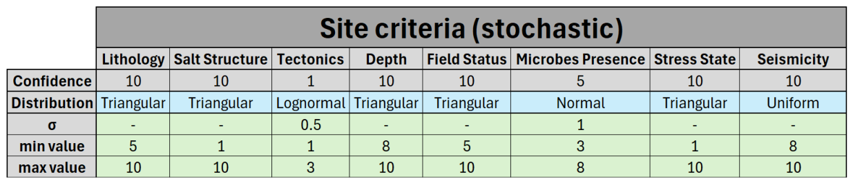
Figure 7.
Front-end implementation of the Dynamic-data input block used to define the cavern clusters of the evaluated site. The “Site information” Table contains the “Caverns Cluster Current status” Table, in which each row corresponds to a different cavern cluster. For each cluster, the table reports the Caverns number, Max Capacity/cavern, Leaching/cavern, Fracture P/cavern, Temperature/cavern, Depth/cavern, and Cushion Gas P/Cavern inputs used to define the geometrical and operating conditions of the cavern system.
Figure 7.
Front-end implementation of the Dynamic-data input block used to define the cavern clusters of the evaluated site. The “Site information” Table contains the “Caverns Cluster Current status” Table, in which each row corresponds to a different cavern cluster. For each cluster, the table reports the Caverns number, Max Capacity/cavern, Leaching/cavern, Fracture P/cavern, Temperature/cavern, Depth/cavern, and Cushion Gas P/Cavern inputs used to define the geometrical and operating conditions of the cavern system.

Figure 8.
Front-end implementation of the Operator’s-data input block. The interface defines the required Injected mass, the Injection Stream Mixture, and the infrastructure-related inputs, Hub Distance used in the site assessment. The Injected mass field specifies the target hydrogen quantity, while the Injection Stream Mixture Table defines the composition of the injected stream through the individual component fractions. The Hub Distance Table contains the producer-to-site distance indicator, , and the site-to-consumer distance indicator, , which characterize the infrastructure proximity of the evaluated site and are subsequently used in the final-ranking calculation.
Figure 8.
Front-end implementation of the Operator’s-data input block. The interface defines the required Injected mass, the Injection Stream Mixture, and the infrastructure-related inputs, Hub Distance used in the site assessment. The Injected mass field specifies the target hydrogen quantity, while the Injection Stream Mixture Table defines the composition of the injected stream through the individual component fractions. The Hub Distance Table contains the producer-to-site distance indicator, , and the site-to-consumer distance indicator, , which characterize the infrastructure proximity of the evaluated site and are subsequently used in the final-ranking calculation.
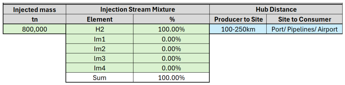
Figure 9.
Representative criterion-level worksheet for Lithology. , and are shown in the “Scoring Framework Table” at the top left, while and are shown in the “Data Confidence Categories” at the bottom left. The admissible , combinations are handled in the “Inclusion Based on Scoring Framework and Data Confidence” Table at the top right, following the inclusion–exclusion logic described in Table A4 of the Appendix. The “Deterministic Score Results” Table at the bottom right reports the Score, , and Confidence Score, , together with the resulting Final Score, , which is subsequently multiplied by the corresponding during the aggregation of the overall .
Figure 9.
Representative criterion-level worksheet for Lithology. , and are shown in the “Scoring Framework Table” at the top left, while and are shown in the “Data Confidence Categories” at the bottom left. The admissible , combinations are handled in the “Inclusion Based on Scoring Framework and Data Confidence” Table at the top right, following the inclusion–exclusion logic described in Table A4 of the Appendix. The “Deterministic Score Results” Table at the bottom right reports the Score, , and Confidence Score, , together with the resulting Final Score, , which is subsequently multiplied by the corresponding during the aggregation of the overall .
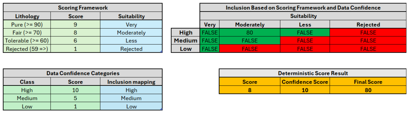
Figure 10.
Summary of the deterministic and stochastic Static-assessment results for the evaluated site. The left-hand Table reports, for each of the eight Static criteria, the , Crit score, , Confidence value, , Weights, , Scoring value, and corresponding relative Contribution to the aggregated . The right-hand “Results” Table reports the resulting Determinsitc, together with the P90, P50, P10, ( arithmetic Mean, and Geomean, geometric mean obtained from the stochastic assessment.
Figure 10.
Summary of the deterministic and stochastic Static-assessment results for the evaluated site. The left-hand Table reports, for each of the eight Static criteria, the , Crit score, , Confidence value, , Weights, , Scoring value, and corresponding relative Contribution to the aggregated . The right-hand “Results” Table reports the resulting Determinsitc, together with the P90, P50, P10, ( arithmetic Mean, and Geomean, geometric mean obtained from the stochastic assessment.
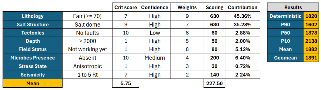
Figure 11.
Criterion-level decomposition of the deterministic Static assessment. (a) Criterion-level weighted contributions to the deterministic Static score. Weighted deterministic score obtained for each Static criterion after consideration of the selected category, , Confidence value, , and Importance weight, . (b) Relative contribution of each Static criterion to the deterministic Static score. Corresponding relative Contribution of each criterion to the overall . The mean value is included as a common reference in both representations.
Figure 11.
Criterion-level decomposition of the deterministic Static assessment. (a) Criterion-level weighted contributions to the deterministic Static score. Weighted deterministic score obtained for each Static criterion after consideration of the selected category, , Confidence value, , and Importance weight, . (b) Relative contribution of each Static criterion to the deterministic Static score. Corresponding relative Contribution of each criterion to the overall . The mean value is included as a common reference in both representations.
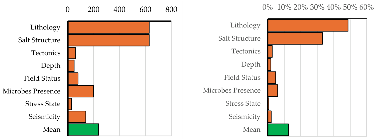
Figure 12.
Cumulative probability distribution of the stochastic Static score obtained from the Monte Carlo assessment. ().
Figure 12.
Cumulative probability distribution of the stochastic Static score obtained from the Monte Carlo assessment. ().
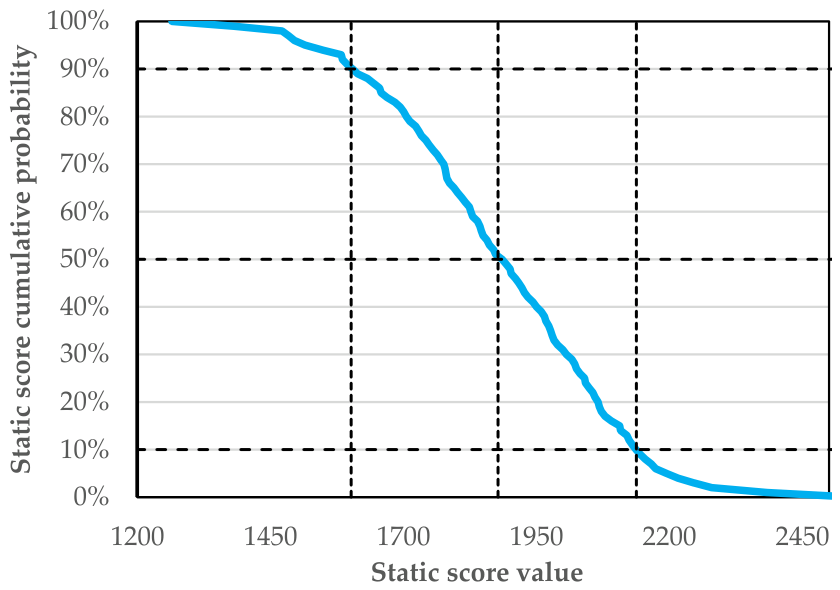
Figure 13.
Front-end configuration of the Importance weights assigned to the final-ranking components. The “Importance [0–10]” row allows the user to define the relative influence the Deterministic score, , the selected P50 (Stochastic) score, , the associated Uncertainty range (P10-P90), , the Fill Factor, , the Recovery Factor, , and the Hub Distance indicators and . on the resulting Final Score, .
Figure 13.
Front-end configuration of the Importance weights assigned to the final-ranking components. The “Importance [0–10]” row allows the user to define the relative influence the Deterministic score, , the selected P50 (Stochastic) score, , the associated Uncertainty range (P10-P90), , the Fill Factor, , the Recovery Factor, , and the Hub Distance indicators and . on the resulting Final Score, .

Figure 14.
Final site-ranking results, including the Static, engineering, infrastructure, and weighted scoring components. The left-hand Table reports the site-specific outputs for the Deterministic score, , the selected P50 (Stochastic) score, , the associated Uncertainty range (P10-P90), , the Fill Factor, , the Recovery Factor, , producer-to-site distance, Hub Distance (PS), , and site-to-consumer distance, Hub Distance (SC), . The central Table reports the corresponding numerical Score, assigned Weights, , weighted Scoring value, and relative Contribution of each component, while the right-hand “Final Score” Table reports the resulting .
Figure 14.
Final site-ranking results, including the Static, engineering, infrastructure, and weighted scoring components. The left-hand Table reports the site-specific outputs for the Deterministic score, , the selected P50 (Stochastic) score, , the associated Uncertainty range (P10-P90), , the Fill Factor, , the Recovery Factor, , producer-to-site distance, Hub Distance (PS), , and site-to-consumer distance, Hub Distance (SC), . The central Table reports the corresponding numerical Score, assigned Weights, , weighted Scoring value, and relative Contribution of each component, while the right-hand “Final Score” Table reports the resulting .
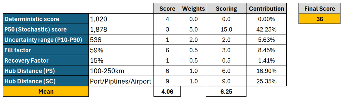
Figure 15.
Potential storage site locations. Dotted curves represent major gas pipeline routes, such as the EastMed pipeline (in red), and the Poseidon pipeline (in pink).
Figure 15.
Potential storage site locations. Dotted curves represent major gas pipeline routes, such as the EastMed pipeline (in red), and the Poseidon pipeline (in pink).
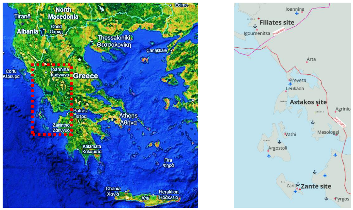
Figure 16.
Static-assessment results for Filiates, presented using the reporting format introduced in Figure 10.
Figure 16.
Static-assessment results for Filiates, presented using the reporting format introduced in Figure 10.
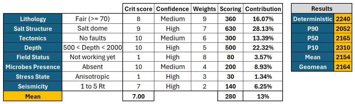
Figure 17.
Static-assessment results for Filiates: (a) relative criterion contributions, following Figure 11b; and (b) cumulative probability distribution of the stochastic Static score, following Figure 12.
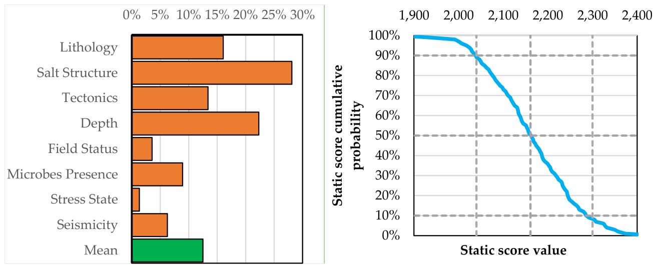
Figure 19.
Static-assessment results for Astakos, presented using the reporting format introduced in Figure 10.
Figure 19.
Static-assessment results for Astakos, presented using the reporting format introduced in Figure 10.
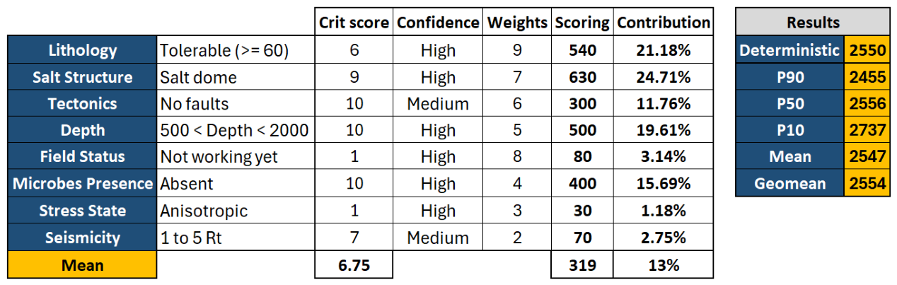
Figure 20.
Static-assessment results for Astakos: (a) relative criterion contributions, following Figure 11b; and (b) cumulative probability distribution of the stochastic Static score, following Figure 12.
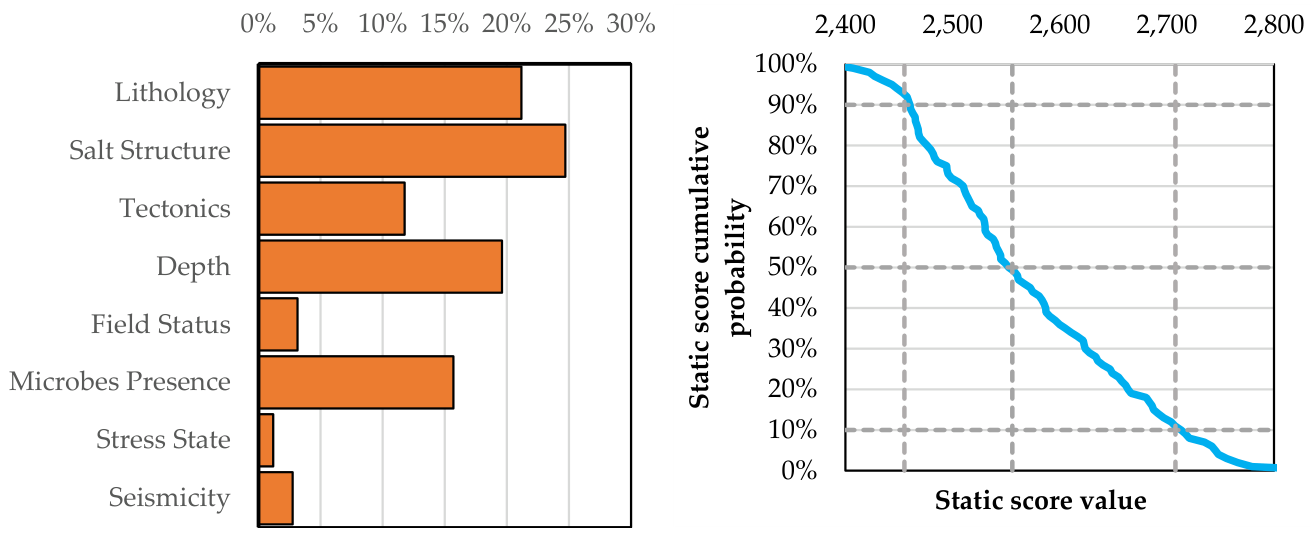
Figure 21.
Final-ranking results for Astakos, presented using the reporting format introduced in Figure 14.
Figure 21.
Final-ranking results for Astakos, presented using the reporting format introduced in Figure 14.
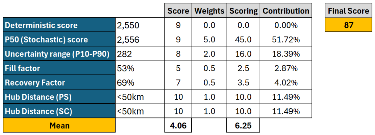
Figure 22.
Static-assessment results for Zante, presented using the reporting format introduced in Figure 10.
Figure 22.
Static-assessment results for Zante, presented using the reporting format introduced in Figure 10.
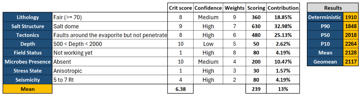
Figure 23.
Static-assessment results for Zante: (a) relative criterion contributions, following Figure 11b; and (b) cumulative probability distribution of the stochastic Static score, following Figure 12.
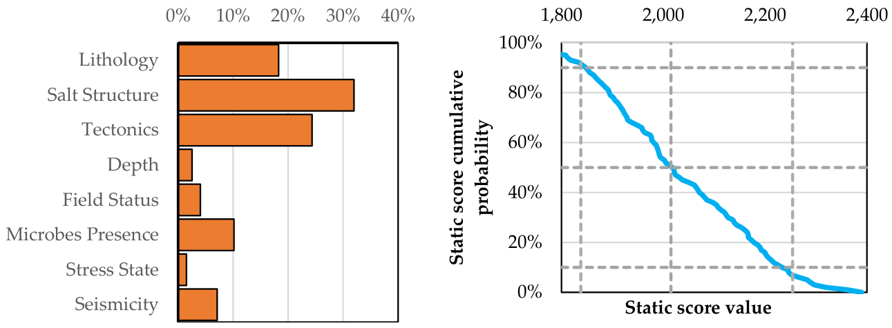
Figure 24.
Final-ranking results for Zante, presented using the reporting format introduced in Figure 14.
Figure 24.
Final-ranking results for Zante, presented using the reporting format introduced in Figure 14.
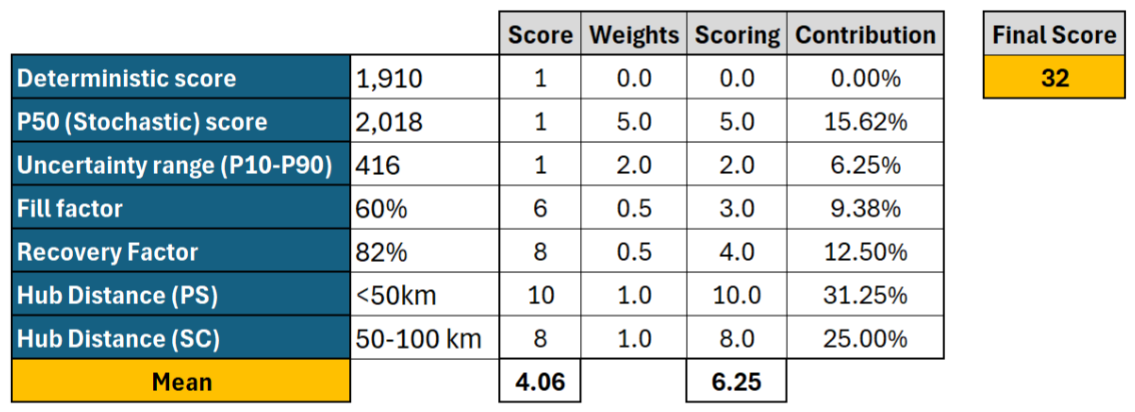
Figure 25.
Comparison of the cumulative probability distributions of the stochastic Static score for Filiates, Astakos, and Zante under the common case-study configuration.
Figure 25.
Comparison of the cumulative probability distributions of the stochastic Static score for Filiates, Astakos, and Zante under the common case-study configuration.
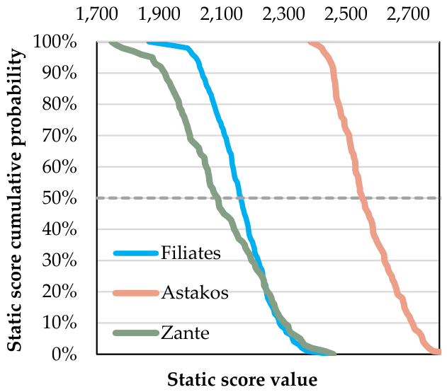
Table 1.
Summary of the , , , , , and , for the three candidate sites under the common assessment scenario.
Table 1.
Summary of the , , , , , and , for the three candidate sites under the common assessment scenario.
| Site | ||||||
|---|---|---|---|---|---|---|
| Astakos | 2,550 | 2,556 | 282 | 53% | 69% | 87 |
| Filiates | 2,240 | 2,165 | 257 | 64% | 92% | 59 |
| Zante | 1,910 | 2,018 | 416 | 60% | 82% | 32 |
Disclaimer/Publisher’s Note: The statements, opinions and data contained in all publications are solely those of the individual author(s) and contributor(s) and not of MDPI and/or the editor(s). MDPI and/or the editor(s) disclaim responsibility for any injury to people or property resulting from any ideas, methods, instructions or products referred to in the content. |
© 2026 by the authors. Licensee MDPI, Basel, Switzerland. This article is an open access article distributed under the terms and conditions of the Creative Commons Attribution (CC BY) license (http://creativecommons.org/licenses/by/4.0/).
Copyright: This open access article is published under a Creative Commons CC BY 4.0 license, which permit the free download, distribution, and reuse, provided that the author and preprint are cited in any reuse.