

Submitted:
07 September 2026
Posted:
08 September 2026
You are already at the latest version
Abstract
Although non-LTE prominence diagnostics have been widelystudied, the impactof realistic 3D velocity fields on prominence emissions remains poorly explored. In this study, we utilize a 2D non-LTE radiative transfer code combined with a 3D MHD model to synthesize HI Lyα and Hα emissions in an eruptive prominence. Incorporating full 3D velocities into the non-LTE calculations reveals three main findings: (1) small-scale motions (∼10kms−1) produce noticeable Doppler dimming in Lyα, whereas Doppler brightening in Hα is less pronounced; (2) Lyα line-center Doppler shifts trace plasma flows in the prominence-corona transition region (PCTR), while Hα line-center shifts reflect line-of-sight integrated signals over a larger range of depths; and (3) Lyα spectral widths depend on PCTR dynamics and temperature, whereas Hα line widths are dominated by optical depth effects. Accounting for 3D velocity fields significantly complicates prominence spectral diagnostics, underscoring the need for further detailed modeling.
Keywords:
Sun
; filaments
; prominences
; techniques
; spectroscopic
; line
; profiles
; radiative transfer
1. Introduction
In solar physics, magnetohydrodynamics (MHD) and radiative transfer theory represent the two primary theoretical pillars required to understand and interpret the solar atmosphere. To validate MHD simulations against observations, forward modeling is necessary to synthesize observables (for a review, see Liakh & Jenkins [1]). For the solar corona, the primary site of large-scale solar eruptions and the solar wind, forward modeling approaches generally fall into two categories: “approximate forward modeling” [2,3,4,5,6,7] and detailed “non-LTE modeling” [8,9,10], where non-LTE denotes departures from local thermodynamic equilibrium. Although the optically thin approximation is widely employed in forward modeling, incorporating empirical relations derived from non-LTE models allows approximate methods to account for essential radiative transfer processes such as photoabsorption [7,11,12]. Nevertheless, approximate forward modeling typically relies on two major simplifications: (1) neglecting the influence of the radiation field on atomic level populations and plasma parameters, and (2) performing 1D integrations along individual lines of sight (LOS), thereby treating each sightline independently of its 3D surroundings. Furthermore, the incident radiation from the underlying solar disk is often omitted, except in specific cases such as K-corona and Ly emission modeling [5].
The non-LTE approach is essential for accurately modeling chromospheric and chromosphere-like plasma—such as solar prominences—and their corresponding spectral emissions. Non-LTE method accounts for non-local atomic–radiation coupling by self-consistently solving the equations of radiative transfer and statistical equilibrium. For prominence modeling, incident radiation from the solar disk and surrounding corona must be included as boundary conditions [13,14]. A complete treatment ideally incorporates frequency redistribution effects (such as partial frequency redistribution, PRD) and full 3D spatial coupling. However, beyond the severe computational cost of non-LTE modeling, existing non-LTE codes often rely on idealized geometric configurations that prevent direct ingestion of 3D numerical MHD datacubes, thereby hindering the widespread adoption of comprehensive non-LTE forward modeling in solar physics.
Bulk mass motions play a crucial role not only in producing Doppler shifts of spectral lines, but also in modulating line intensities—a phenomenon known as the Doppler dimming or brightening effect [15,16]. Although both radial and horizontal mass motions contribute to these intensity variations [17], the physical mechanism is most straightforwardly explained assuming purely radial motion relative to the solar surface. Bulk motion of the plasma Doppler-shifts the incident profile of a chromospheric spectral line as seen by the moving atom. When the incident radiation features an emission profile (such as H i Ly), the Doppler misalignment between the incident radiation and the local absorption profile leads to Doppler dimming. Conversely, when the incident radiation features an absorption profile (such as H), radial bulk motion shifts the absorption profile into stronger off-center continuum or wing radiation, resulting in Doppler brightening. The Doppler dimming effect of Ly has been widely utilized to infer the velocity and temperature structure of coronal mass ejections (CMEs) [18] as well as the fast and slow solar wind [19,20].
Observations frequently reveal complex dynamic flows during prominence eruptions [21,22]. In the 3D MHD numerical simulations by Y. Fan [23,24,25,26], bulk mass motions within the flux rope—spanning from emergence to eruption—exhibit thermal condensation, plasma evaporation into prominence “horns”, and mass draining along the flux rope legs.
In this work, we couple the 3D MHD simulation results of Fan & Liu [25] with the 2D non-LTE radiative transfer code CYMA2DV1 [27,28] to synthesize H i Ly and H spectral emissions in an eruptive prominence. Developed by P. Gouttebroze, CYMA2DV models cylindrical prominence configurations while incorporating full 3D velocity vectors. Synthetic H i Ly forward modeling of this specific prominence–cavity system was previously conducted by Zhao et al. [29] using both optically thin approximations and 1D non-LTE modeling, while the underlying eruption mechanisms were investigated by Liu & Su [30].
2. Materials and Methods
Although observations suggest that a solar prominence is composed of numerous fine threads [31], we treat the cross-section of the simulated prominence [25] as a compact circular cylinder for two main reasons: (1) existing multi-thread radiative transfer models typically neglect the mutual attenuation of incident radiation between threads, assuming an identical incident radiation field for all individual threads [32,33,34]; and (2) the simulated prominence mass remains concentrated in a single compact structure rather than being fragmented prior to the fast-rise phase of the eruption.
2.1. MHD Model
The MHD simulation of the magnetic flux rope was performed by Fan & Liu [25], who incorporated fully ionized hydrogen gas, empirical coronal heating, optically thin radiative losses, and field-aligned thermal conduction. Because the CYMA2DV code requires a cylindrical prominence thread geometry, and the prominence sheet increasingly departs from an idealized cylinder during eruption, we analyze two snapshots at the onset of the eruption: steps 180 and 184.
The original MHD output is defined in spherical coordinates, containing temperature, plasma number density, gas pressure, 3D velocity fields, and magnetic fields. We interpolated the datacubes onto a Cartesian coordinate system with a uniform spatial resolution of solar radii () per pixel (approximately ). The orientation of the Cartesian axes (X, Y, Z) follows the coordinate setup of Zhao et al. [29]: the X-axis lies roughly along the prominence main axis, the Y-axis points along the radial direction from the solar surface, and the Z-axis is perpendicular to the prominence sheet. Figure 1a and Figure 1e display the temperature maps in the X–Y plane for the two steps, obtained by taking the minimum temperature along the Z direction. Density distributions in the X–Z plane at three different heights (Y) are presented in Figure 1b–d and Figure 1f–h. As illustrated in Figure 1, the prominence vertical extent in the X–Y plane () is significantly larger than its horizontal width in the X–Z plane (), indicating a thin plasma sheet rather than a loop with a circular cross-section. Additionally, the main body of the prominence sheet () exhibits a larger thickness compared to its lower legs ().
In the original MHD simulation, to prevent the pressure scale height from becoming unresolvably small under the grid resolution limit, radiative cooling was artificially suppressed for temperatures below [23]. Consequently, the minimum plasma temperature in the numerical domain remains around —roughly an order of magnitude higher than typical observational values for prominence cores (–) [21,35,36]. To account for this, we scaled the temperature down by a factor of 10 prior to non-LTE radiative transfer calculations. Due to this artificial temperature floor, although a transition layer between the prominence mass and the ambient corona is present in the simulation, its thermal structure differs slightly from the canonical prominence-corona transition region (PCTR) with temperatures below a few hundred .
2.2. Radiative Transfer Code
In this study, we employ the non-LTE radiative transfer code CYMA2DV [27,28] to synthesize the emergent H i Ly and H line profiles from the modeled prominence. Only hydrogen element is considered with a 5-level plus continuum model, and complete frequency redistribution (CRD) is used for both hydrogen lines and continua. CYMA2DV is designed for cylindrical structures embedded in the solar corona, accounting for a two-dimensional spatial cross-section (perpendicular to the cylinder’s symmetry axis) and arbitrary 3D velocity fields. Under this geometry, the cylinder is assumed to be infinitely long, illuminated exclusively at its outer boundary by incident solar disk radiation. The cylindrical structural model with a PCTR is defined by several core parameters: constant gas pressure P, inclination angle , height above the solar surface H, radius of the isothermal core , total cylinder radius , core temperature , and external PCTR boundary temperature . The temperature distribution within the PCTR varies logarithmically as a function of radial distance r:
The microturbulent velocity is assumed to be uniform at .
CYMA2DV uses a local Cartesian coordinate system defined relative to the cylinder: the z-axis lies along the cylinder axis, the y-axis aligns with the LOS, and the x–z plane forms the plane of sky (POS). The 3D velocity vectors within the 2D spatial domain are defined in this local frame. We modified the original code to import externally interpolated 3D velocity fields, thereby enabling direct ingestion of the plasma velocity vectors computed by the 3D MHD model.
2.3. Extracting Prominence Parameters from the MHD Model
To couple the MHD simulation results with the CYMA2DV forward modeling code, the continuous prominence structure is approximated as a sequence of circular cylindrical cross-sections, each characterized by distinct radii, locations, and spatial inclination angles. The extraction of local prominence input parameters involves four main steps: (1) tracing the smoothed prominence axis, (2) cutting transverse cross-sectional slices perpendicular to the axis, (3) identifying the cross-sectional centers, and (4) extracting the local thermodynamic and kinematic parameters.
The prominence main axis was identified using the minimum temperature path in the X–Y plane and smoothed using a 1-pixel Gaussian kernel (Figure 2a). The cylinder axis required by CYMA2DV is defined along the local tangent to this smoothed axis, which uniquely determines both the cross-sectional orientation and the inclination angle . Panels (b) and (c) of Figure 2 show the resulting temperature and gas pressure distributions within a representative cross-section. To define the center and boundary of the cool core, only grid cells with temperatures below are selected: the core center is set as the spatial centroid of these cold pixels, the core radius is defined as half the core thickness along the local y-direction, and the PCTR thickness is fixed at . We adopt a fixed PCTR thickness for two primary reasons: (1) the MHD grid resolution cannot fully resolve an empirical non-LTE PCTR spanning from to several hundred , and (2) an excessively thick PCTR generates artificially strong emission at the prominence top edge due to the assumed cylindrical symmetry. The spatial height H of each slice is determined directly by the centroid position of the cross-section along the Y-axis.
Once the cross-sectional position and spatial extent are defined, the core temperature and gas pressure P are extracted as the median values within the central region of the cool core, followed by spatial smoothing along the prominence axis. The temperature at the outer boundary of the PCTR, , is fixed at . Finally, the 3D velocity vectors within each 2D cross-section are extracted from the MHD domain and interpolated onto the CYMA2DV spatial grid.
The observed decrease in gas pressure near the outer edge of the cool core is primarily driven by runaway radiative cooling and dynamic plasma motions [25]. The gas pressure rises again across the PCTR as temperature increases toward coronal values. This behavior reduces the pressure contrast between the core and the surrounding corona, maintaining overall pressure balance for a prominence core that is roughly 100 times cooler and denser than the ambient coronal environment.
3. Results
To evaluate the impact of velocity fields on prominence spectral emissions, we first present the forward modeling results obtained by incorporating the full 3D velocity fields, and subsequently compare them against static benchmark cases where all velocity components are set to zero.
3.1. Modeling with 3D Velocity Fields
Prominence line emission is primarily governed by local plasma temperature, gas pressure, spatial thickness, 3D velocity vectors, and height above the solar limb. Figure 3 displays the axial distributions of these input parameters (excluding spatial height) along with the resulting synthetic integrated line intensities for Ly and H at steps 180 (blue solid curves) and 184 (red dashed curves). Across the two time steps, the core temperature varies within a narrow range between 7230 and , while the gas pressure decreases slightly along time (). Conversely, the spatial thickness near the prominence main body expands significantly, with the core radius increasing by approximately . These structural variations reflect ongoing prominence expansion and continuous plasma condensation. Note that the 3D velocity components () in Figure 3 are defined in the local cylindrical reference frame. The elevated values near the main body reflect the eruptive expansion; at the prominence core center remain small; and the large magnitude of near the legs captures field-aligned mass draining.
Comparing the spatial distribution of plasma parameters with synthetic emissions at step 180 reveals distinct behavior between the two spectral lines. The Ly intensity closely tracks the coupled variation of temperature and pressure, whereas H intensity correlates primarily with the combination of gas pressure and cylinder radius. For Ly, two shallow intensity dips occur near slices (transitioning from the legs to the main body), which result from temperature drops. In contrast, the dependence of H emission on pressure and radius is consistent with the established proportional relationship between H intensity and emission measure, [37], where and denote the hydrogen and electron number densities, and l represents path length along the LOS. These coupling relationships also explain the temporal evolution between steps 180 and 184, though the rise of velocities introduces additional complexity. As condensation proceeds, both core temperature and pressure in the prominence main body decline, causing a dominant decrease in Ly intensity. Conversely, H emission near the main body increases due to the marked expansion of the prominence core radius.
We synthesize 2D prominence images by combining the emergent spectral intensity from each individual cross-sectional slice along the prominence axis. From the emergent line profiles, we also construct spatial maps of Doppler velocity and full-width-at-half-maximum (FWHM). The resulting synthetic intensity, Doppler shift, and line-width maps for both Ly and H at steps 180 and 184 are presented in Figure 4, Figure 5 and Figure 6.
The spatial intensity distributions of Ly and H exhibit clear differences. The Ly emission is brightest along the prominence boundaries, where the PCTR path length integrated along the line of sight (LOS) is longest. In contrast, peak H emission occurs near the base of the prominence main body, displaying a smoother spatial distribution characteristic of resonant scattering of disk radiation by the cool core. Their temporal evolution from step 180 to 184 is likewise distinct: as shown in Figure 3, Ly intensity decreases slightly, whereas H exhibits a pronounced overall enhancement.
Because the synthesized Ly and H spectral profiles are simpler than observations, we determine line-center positions using an extremum-finding algorithm [21,36,38]: identifying the peak position for single-peaked profiles or the central reversal minimum for self-reversed profiles. Doppler shifts of these line centers are then converted into LOS velocity maps. As shown in Figure 5, Ly exhibits widespread redshifts (motion away from the observer), and we will see that the redshifts are caused by converging flows. In contrast, H shows localized blueshifts alongside dominant redshifts. Note that line centers are formed at shallower optical depths than the line wings. Alternative methods, such as center-of-gravity estimation or bisector shifts at half-maximum [22], capture LOS dynamics at deeper optical depths or provide weighted average motions along the sightline.
The spectral line width—quantified by FWHM in angstroms ()—displays a relatively uniform spatial distribution in Ly, with larger values confined to the PCTR-dominated edges at both steps and near the footpoints at step 184. For H, the main body consistently exhibits broader line widths than the legs. We further examine the physical origins of these spectral features in the following subsection by comparing them against the static benchmark case.
To further investigate the formation mechanisms of prominence emission and assess the impact of 3D velocity fields, Figure 7 and Figure 8 display synthetic intensity images (panels a–b), Doppler velocity maps (e–f), stigmatic spectra along a representative cross-sectional slice (c–d), and internal cross-sectional velocity fields (g–i). White solid lines in panels (a–b) and (e–f) indicate the spatial position of the selected slice, while dotted circles in panels (g–i) outline the boundary of the input cylindrical cross-section. Two accompanying animation files, animation_1.mp4 (step 180) and animation_2.mp4 (step 184), are provided in the online journal material.
The velocity fields shown in Figure 7 and Figure 8 capture complex dynamic plasma motions around and within the cylinder: positive values track eruptive expansion, opposing sign pairs of (along the LOS) capture plasma draining toward magnetic dips during thermal condensation within the prominence–cavity system, and opposing values (along the cylinder axis) represent counter-streaming motions.
3.2. Modeling Without Velocity Fields
With all velocity components set to zero, the resulting synthetic line intensity distributions for Ly and H are presented in Figure 9, while the corresponding intensity ratios between the dynamic and static scenarios are displayed in Figure 10. The intensity ratio maps demonstrate that even moderate bulk mass motions—around for step 180, for step 184, and dominated by radial velocities—can induce significant variations in emergent spectral line intensities. Specifically, the Ly intensity decreases, whereas the H intensity exhibits Doppler brightening because the incident chromospheric H profile is an absorption feature.
Furthermore, the contrast between steps 180 and 184 indicates that H i Ly intensity is more sensitive to small-amplitude velocity variations than H. As plasma velocities increase from step 180 to 184, Doppler dimming in Ly becomes further accentuated only within two localized regions. Conversely, Doppler brightening in H across the prominence main body exhibits a marked overall enhancement that decreases with spatial height.
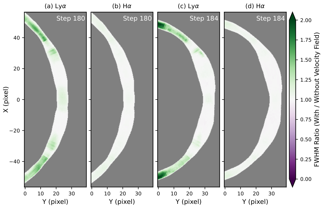
The corresponding FWHM spectral width distributions for the static benchmark case are shown in Figure 11, with the FWHM ratio maps ( relative to ) displayed in Figure 12. For the Ly line, enhanced FWHM values persist along the outer PCTR boundaries even in the absence of velocity fields, confirming that line broadening near the prominence edges is primarily thermal in origin. Spatially complex velocity distributions predominantly contribute to Ly line broadening along the prominence legs, most notably near the footpoints at step 184.
For the H line, bulk velocity fields exert a minimal influence on spectral width. Because temperature generally decreases from the legs toward the prominence main body, the larger H spectral widths observed in the main body cannot be attributed to thermal broadening. Ruling out thermal and velocity-driven effects, the spatial variations in H line width are primarily governed by optical depth: as prominence spatial thickness increases, the optical depth, total intensity, and FWHM of the self-absorbed H line increase accordingly.
4. Discussion
4.1. Prominence Brightness
Synthetic images of integrated line intensity demonstrate that the PCTR plays a crucial role in regulating Ly emission, whereas resonant scattering of underlying solar disk radiation is important for the H intensity. Because Doppler dimming and brightening effects are intimately tied to resonant scattering, one might expect H emission to be more sensitive to bulk plasma motions than Ly. This expectation aligns with 1D non-LTE calculations employing isobaric and isothermal prominence models [15,16]. However, our 2D non-LTE prominence modeling including a PCTR reveals significant Ly Doppler dimming even when typical radial velocities are only around . Counter-streaming flows within the PCTR may contribute to this Ly Doppler dimming; nevertheless, radial components dominate the overall 3D velocity field. Dedicated parametric studies are required to confirm this mechanism.
Additionally, our idealized, cylindrically symmetric prominence model produces enhanced Ly brightness along both the top and bottom PCTR boundaries. In contrast, observational observations do not typically exhibit enhanced Ly emission at the prominence top. Under the combined influence of gravity and magnetic fields, real prominences develop vertical asymmetry, yielding thermodynamic distributions across the PCTR that differ substantially from symmetric cylindrical models.
4.2. LOS Velocities and Spectral Line Widths
The LOS velocities derived from synthetic spectral line profiles near the prominence main body are primarily driven by converging flows along with the prominence condensations. Because Ly has a much higher optical depth than H, Ly profiles are predominantly redshifted, capturing PCTR dynamics on the side facing the observer. Near the prominence legs, reflects localized turbulence associated with eruptive expansion and mass draining (see accompanying animations). Surprisingly, the Doppler shifts of synthetic H profiles are anti-correlated with the dominant velocity component across the legs.
This unexpected behavior prompts us to examine the role of axial mass motion ( near the legs) on profile shifts. From the perspective of the falling plasma along the legs, incident disk radiation is blueshifted; because the incident solar H spectrum is an absorption feature, this shift enhances the red wing of the scattered profile. However, this interpretation faces two key challenges: (1) under this scenario, emergent profiles from both legs should be consistently redshifted, and (2) frequency coupling between incident and scattered profiles is weak under the CRD approximation.
A related phenomenon is the pronounced response of H intensity along the legs, as well as Ly spectral widths, to the 3D velocity field. As shown in Figure 7, velocity fields enhance H emission near the legs even at step 180, when velocity-driven effects remain negligible across the main body. Similarly, Figure 8 indicates that velocity fields broaden Ly profiles originating from the legs while exerting a weaker influence on the main body. Fully untangling these localized spectral responses will require dedicated single-slice forward modeling, which we reserve for future work.
5. Conclusions
In this work, we synthesize emergent H i Ly and H line emissions by applying a 2D non-LTE radiative transfer code (CYMA2DV) to an eruptive prominence model derived from 3D MHD simulations. The simulated prominence is decomposed into a sequence of cylindrical cross-sections characterized by distinct spatial inclination angles, radii, and thermodynamic properties, but featuring a uniform PCTR thickness. Ingesting the 3D velocity fields directly from the MHD model yields several key findings:
- 1.
- Ly exhibits pronounced Doppler dimming across the entire prominence structure, even at relatively low bulk speeds of . Under identical velocity fields, H Doppler brightening is comparatively modest and concentrated primarily near the legs and the lower boundary of the main body.
- 2.
- The line-center Doppler shifts of the emergent Ly profiles are predominantly governed by PCTR dynamics on the observer-facing side due to high optical depth, whereas emergent H Doppler shifts receive significant contributions from deeper plasma layers within the prominence core.
- 3.
- The spectral line width of Ly is determined mainly by high PCTR temperatures and spatially varying bulk mass motions. In contrast, H line broadening is primarily governed by optical depth variations (self-absorption) under the assumed constant microturbulent velocity of .
The complex coupling among the 3D velocity field, cylindrical geometry, and non-uniform thermal structures highlights the need for dedicated parametric non-LTE studies. Future numerical experiments are required to clarify: (1) whether Ly or H intensity is intrinsically more sensitive to bulk plasma motions across a broader range of velocities; (2) the precise mapping between observed H Doppler shifts and complex internal mass flows; and (3) why Ly spectral widths originating from the prominence legs exhibit greater sensitivity to bulk velocity fields than those from the main body.
Supplementary Materials
The following supporting information can be downloaded at the website of this paper posted on Preprints.org.
Author Contributions
Conceptualization, Li Feng; Methodology, Jianchao Xue, Li Feng and Yiliang Li; Software, Jianchao Xue, Yiliang Li and Jean-Claude Vial; Validation, Jianchao Xue, Li Feng and Jean-Claude Vial; Formal analysis, Jianchao Xue, Li Feng, Yiliang Li and Jie Zhao; Investigation, Jianchao Xue; Writing – original draft, Jianchao Xue; Writing – review & editing, Li Feng, Yiliang Li, Jean-Claude Vial, Jie Zhao and Hui Li; Supervision, Li Feng, Jean-Claude Vial and Hui Li; Project administration, Li Feng; Funding acquisition, Li Feng. All authors have read and agreed to the published version of the manuscript.
Funding
This work is supported by the Strategic Priority Research Program of the Chinese Academy of Sciences, Grant No. XDB0560000, NSFC grant No.12233012, National Key R&D Program of China 2022YFF0503003 (2022YFF0503000), the project of Solar Polar Observatory GJ11020204, NSFC grant No.12203102. J.X. is funded by Basic Research Program of Jiangsu BK20251705.
Data Availability Statement
The MHD model data were provided by Y.Fan. The CYMA2DV code is available at https://idoc.osups.universite-paris-saclay.fr/medoc/tools/radiative-transfer-codes/.
Conflicts of Interest
The authors declare no conflicts of interest.
References
- Liakh, V.; Jenkins, J. Numerical Modeling of Prominences and Coronal Rain with the MPI-AMRVAC Code. Sol. Phys. 2025, 300, 147. [Google Scholar] [CrossRef] [PubMed]
- Xia, C.; Keppens, R.; Antolin, P.; Porth, O. Simulating the in Situ Condensation Process of Solar Prominences. ApJ 2014, 792, L38. [Google Scholar] [CrossRef]
- Gibson, S.; Kucera, T.; White, S.; Dove, J.; Fan, Y.; Forland, B.; Rachmeler, L.; Downs, C.; Reeves, K. FORWARD: A toolset for multiwavelength coronal magnetometry. Front. Astron. Space Sci. 2016, 3, 8. [Google Scholar] [CrossRef]
- Zhao, X.; Xia, C.; Van Doorsselaere, T.; Keppens, R.; Gan, W. Forward Modeling of SDO/AIA and X-Ray Emission from a Simulated Flux Rope Ejection. ApJ 2019, 872, 190. [Google Scholar] [CrossRef]
- Ying, B.; Shi, G.; Feng, L.; Lu, L.; Xue, J.; Li, S.; Gan, W.; Li, H. Parameter Effects on the Total Intensity of H I Lyα Line for a Modeled Coronal Mass Ejection and Its Driven Shock. Sol. Phys. 2024, 299, 92. [Google Scholar] [CrossRef]
- Sorokina, D.; Van Doorsselaere, T.; Lloveras, D.G.; Linan, L.; Poedts, S. FoMo white-light tool: Coupling with state-of-the-art numerical models. A&A 2025, 701, A166. [Google Scholar] [CrossRef]
- Fu, W.; Ni, Y.; Zhang, Y.; Chen, G.; Wang, B.; Guo, J.; Xing, C.; Guo, Y.; Ding, M. Radiation Synthesis Tools: Arbitrary Perspective Multiwavelength Radiation Synthesis for Solar Magnetohydrodynamic Simulations. ApJ 2026, 1004, 166. [Google Scholar] [CrossRef]
- Jenkins, J.M.; Osborne, C.M.J.; Keppens, R. 1.5D non-LTE spectral synthesis of a 3D filament and prominence simulation. A&A 2023, 670, A179. [Google Scholar] [CrossRef]
- Pietrow, A.G.M.; Liakh, V.; Osborne, C.M.J.; Jenkins, J.; Keppens, R. Spectral characteristics of a rotating solar prominence in multiple wavelengths. A&A 2024, 690, L15. [Google Scholar] [CrossRef]
- Osborne, C.M.J.; Sannikov, A. Radiance cascades: a novel high-resolution formal solution for multidimensional non-LTE radiative transfer. RAS Tech. Instrum. 2025, 4, rzae062. [Google Scholar] [CrossRef]
- Heinzel, P.; Gunár, S.; Anzer, U. Fast approximate radiative transfer method for visualizing the fine structure of prominences in the hydrogen Hα line. A&A 2015, 579, A16. [Google Scholar] [CrossRef]
- Gunár, S.; Mackay, D.H. 3D Whole-Prominence Fine Structure Modeling. ApJ 2015, 803, 64. [Google Scholar] [CrossRef]
- Gunár, S.; Schwartz, P.; Koza, J.; Heinzel, P. Quiet-Sun hydrogen Lyman-α line profile derived from SOHO/SUMER solar-disk observations. A&A 2020, 644, A109. [Google Scholar] [CrossRef]
- Gunár, S.; Heinzel, P.; Koza, J.; Schwartz, P. Large Impact of the Mg II h and k Incident Radiation Change on Results of Radiative Transfer Models and the Importance of Dynamics. ApJ 2022, 934, 133. [Google Scholar] [CrossRef]
- Heinzel, P.; Rompolt, B. Hydrogen Emission from Moving Solar Prominences. Sol. Phys. 1987, 110, 171–189. [Google Scholar] [CrossRef]
- Gontikakis, C.; Vial, J.C.; Gouttebroze, P. Spectral diagnostics for eruptive prominences. Sol. Phys. 1997, 172, 189–197. [Google Scholar] [CrossRef]
- Peat, A.W.; Osborne, C.M.J.; Heinzel, P. Doppler dimming and brightening effects in solar prominences. MNRAS 2024, 533, L19–L24. [Google Scholar] [CrossRef]
- Ying, B.; Bemporad, A.; Feng, L.; Lu, L.; Gan, W.; Li, H. Extensive Study of a Coronal Mass Ejection with UV and White-light Coronagraphs: The Need for Multiwavelength Observations. ApJ 2020, 899, 12. [Google Scholar] [CrossRef]
- Romoli, M.; Antonucci, E.; Andretta, V.; Capuano, G.E.; Da Deppo, V.; De Leo, Y.; Downs, C.; Fineschi, S.; Heinzel, P.; Landini, F.; et al. First light observations of the solar wind in the outer corona with the Metis coronagraph. A&A 2021, 656, A32. [Google Scholar] [CrossRef]
- Giordano, S.; Spadaro, D.; Susino, R.; Ventura, R.; Zangrilli, L.; Andretta, V.; De Leo, Y.; Romoli, M.; Teriaca, L.; Uslenghi, M.; et al. Solar wind speed maps from the Metis coronagraph observations. A&A 2025, 701, A56. [Google Scholar] [CrossRef]
- Zhang, P.; Buchlin, É.; Vial, J.C. Launch of a CME-associated eruptive prominence as observed with IRIS and ancillary instruments. A&A 2019, 624, A72. [Google Scholar] [CrossRef]
- Xue, J.; Li, H.; Su, Y. Spectral evolution of an eruptive polar crown prominence with IRIS observations. Front. Phys. 2021, 9, 543. [Google Scholar] [CrossRef]
- Fan, Y. MHD Simulations of the Eruption of Coronal Flux Ropes under Coronal Streamers. ApJ 2017, 844, 26. [Google Scholar] [CrossRef]
- Fan, Y. MHD Simulation of Prominence Eruption. ApJ 2018, 862, 54. [Google Scholar] [CrossRef]
- Fan, Y.; Liu, T. MHD simulation of prominence-cavity system. Front. Astron. Space Sci. 2019, 6, 27. [Google Scholar] [CrossRef]
- Fan, Y. Simulations of Prominence Eruption Preceded by Large-amplitude Longitudinal Oscillations and Draining. ApJ 2020, 898, 34. [Google Scholar] [CrossRef]
- Gouttebroze, P. Radiative transfer in cylindrical threads with incident radiation. III. Hydrogen spectrum. A&A 2006, 448, 367–374. [Google Scholar] [CrossRef]
- Gouttebroze, P. Radiative transfer in cylindrical threads with incident radiation. V. 2D transfer with 3D velocity fields. A&A 2008, 487, 805–813. [Google Scholar] [CrossRef]
- Zhao, J.; Zhang, P.; Gibson, S.E.; Fan, Y.; Feng, L.; Yu, F.; Li, H.; Gan, W.Q. Synthetic Lyman-α emissions for the coronagraph aboard the ASO-S mission. I. An eruptive prominence-cavity system. A&A 2022, 665, A39. [Google Scholar] [CrossRef]
- Liu, T.; Su, Y. Tether-cutting and Overlying Magnetic Reconnections in an MHD Simulation of Prominence-cavity System. ApJ 2021, 915, 55. [Google Scholar] [CrossRef]
- Lin, Y.; Engvold, O.; der Voort, L.R.v.; Wiik, J.E.; Berger, T.E. Thin Threads of Solar Filaments. Sol. Phys. 2005, 226, 239–254. [Google Scholar] [CrossRef]
- Gunár, S.; Heinzel, P.; Anzer, U.; Schmieder, B. On Lyman-line asymmetries in quiescent prominences. A&A 2008, 490, 307–313. [Google Scholar] [CrossRef]
- Labrosse, N.; Rodger, A.S. Radiative transfer in cylindrical threads with incident radiation. VII. Multi-thread models. A&A 2016, 587, A113. [Google Scholar] [CrossRef]
- Heinzel, P.; Gunár, S. Radiative Transfer in Solar Prominences: An Overview and Current Trends. Sol. Phys. 2025, 300, 167. [Google Scholar] [CrossRef]
- Jejčič, S.; Heinzel, P.; Schmieder, B.; Gunár, S.; Mein, P.; Mein, N.; Ruan, G. Non-LTE Inversion of Prominence Spectroscopic Observations in Hα and Mg II h&k lines. ApJ 2022, 932, 3. [Google Scholar] [CrossRef]
- Xue, J.; Zhang, P.; Vial, J.C.; Feng, L.; Zapiór, M.; Curdt, W.; Li, H.; Gan, W. Multiwavelength spectroscopic observations of a quiescent prominence. A&A 2025, 703, A145. [Google Scholar] [CrossRef]
- Gouttebroze, P.; Heinzel, P.; Vial, J.C. The hydrogen spectrum of model prominences. A&AS 1993, 99, 513–543. [Google Scholar]
- Leenaarts, J.; Pereira, T.M.D.; Carlsson, M.; Uitenbroek, H.; De Pontieu, B. The Formation of IRIS Diagnostics. II. The Formation of the Mg II h&k Lines in the Solar Atmosphere. ApJ 2013, 772, 90. [Google Scholar] [CrossRef]
Figure 1.
Snapshots of the simulated prominence. Left column: Minimum temperature distributions along the Z-axis projected onto the X–Y plane. Remaining columns: Density distributions in the X–Z plane at three different altitudes. The top row corresponds to step 180, and the bottom row corresponds to step 184.
Figure 1.
Snapshots of the simulated prominence. Left column: Minimum temperature distributions along the Z-axis projected onto the X–Y plane. Remaining columns: Density distributions in the X–Z plane at three different altitudes. The top row corresponds to step 180, and the bottom row corresponds to step 184.
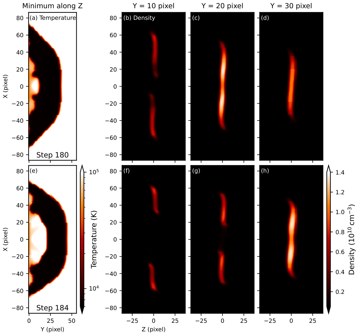
Figure 2.
Determination of prominence parameters for CYMA2DV. Left column: Temperature distribution in the X–Y plane at step 184. The blue curve denotes the traced prominence axis, the white line represents a transverse cross-sectional slice, the solid cyan line indicates the tangent to the axis, and the inclination angle is the acute angle between the tangent line and the Y-axis. Middle column: Spatial distributions of temperature and gas pressure in the cross-sectional plane. Pluses (+) mark the center of the cylindrical cross-section, solid circles denote the boundary of the isothermal core (), and dotted circles represent the outer boundary of the PCTR (). Images are displayed on a linear scale, with minimum and maximum values specified in each panel. Note that this local coordinate system differs from the global MHD domain. Right column: One-dimensional profiles of temperature and gas pressure along the x- and y-axes intersecting the cross-sectional center.
Figure 2.
Determination of prominence parameters for CYMA2DV. Left column: Temperature distribution in the X–Y plane at step 184. The blue curve denotes the traced prominence axis, the white line represents a transverse cross-sectional slice, the solid cyan line indicates the tangent to the axis, and the inclination angle is the acute angle between the tangent line and the Y-axis. Middle column: Spatial distributions of temperature and gas pressure in the cross-sectional plane. Pluses (+) mark the center of the cylindrical cross-section, solid circles denote the boundary of the isothermal core (), and dotted circles represent the outer boundary of the PCTR (). Images are displayed on a linear scale, with minimum and maximum values specified in each panel. Note that this local coordinate system differs from the global MHD domain. Right column: One-dimensional profiles of temperature and gas pressure along the x- and y-axes intersecting the cross-sectional center.
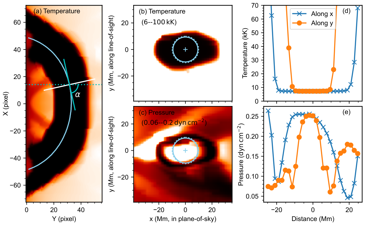
Figure 3.
Extracted input parameters (temperatures , gas pressures P, cylinder radii , and 3D velocity components) together with synthetic integrated intensities of Ly and H plotted along the prominence axis at steps 180 (solid blue lines) and 184 (dashed red lines). Slice numbers increase along the X-axis.
Figure 3.
Extracted input parameters (temperatures , gas pressures P, cylinder radii , and 3D velocity components) together with synthetic integrated intensities of Ly and H plotted along the prominence axis at steps 180 (solid blue lines) and 184 (dashed red lines). Slice numbers increase along the X-axis.
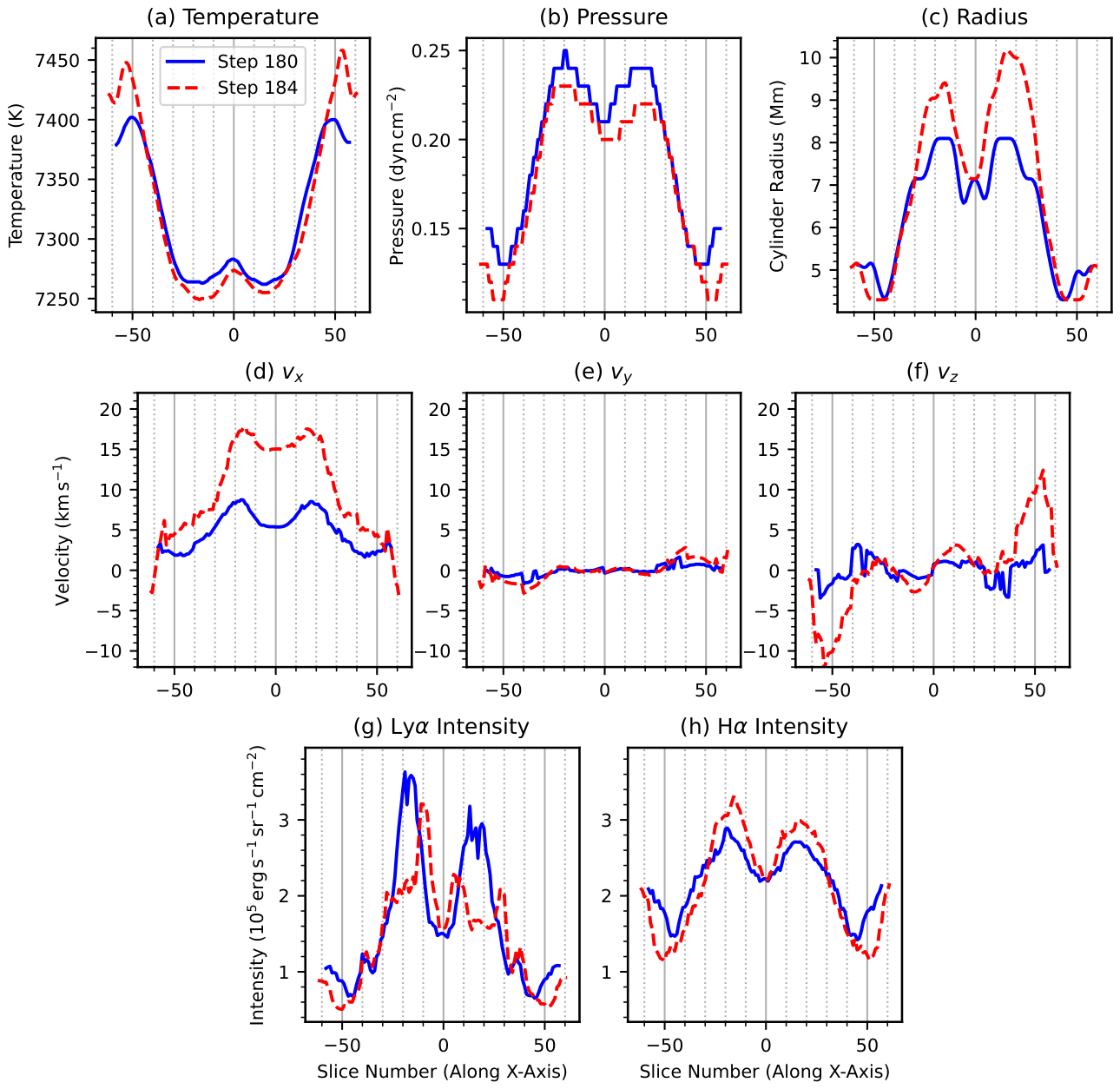
Figure 4.
Spatial distributions of integrated line intensity for Ly and H at steps 180 and 184.
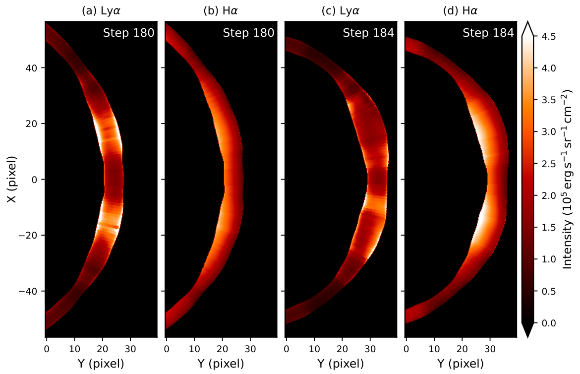
Figure 5.
Doppler (LOS) velocity distributions of Lyα and Hα at steps 180 and 184.
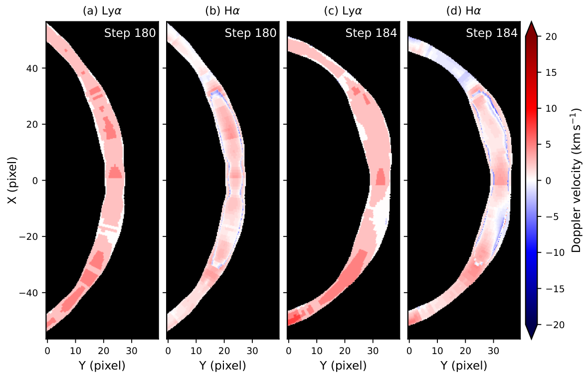
Figure 6.
Full-width-at-half-maximum (FWHM) distributions of Lyα and Hα at steps 180 and 184.
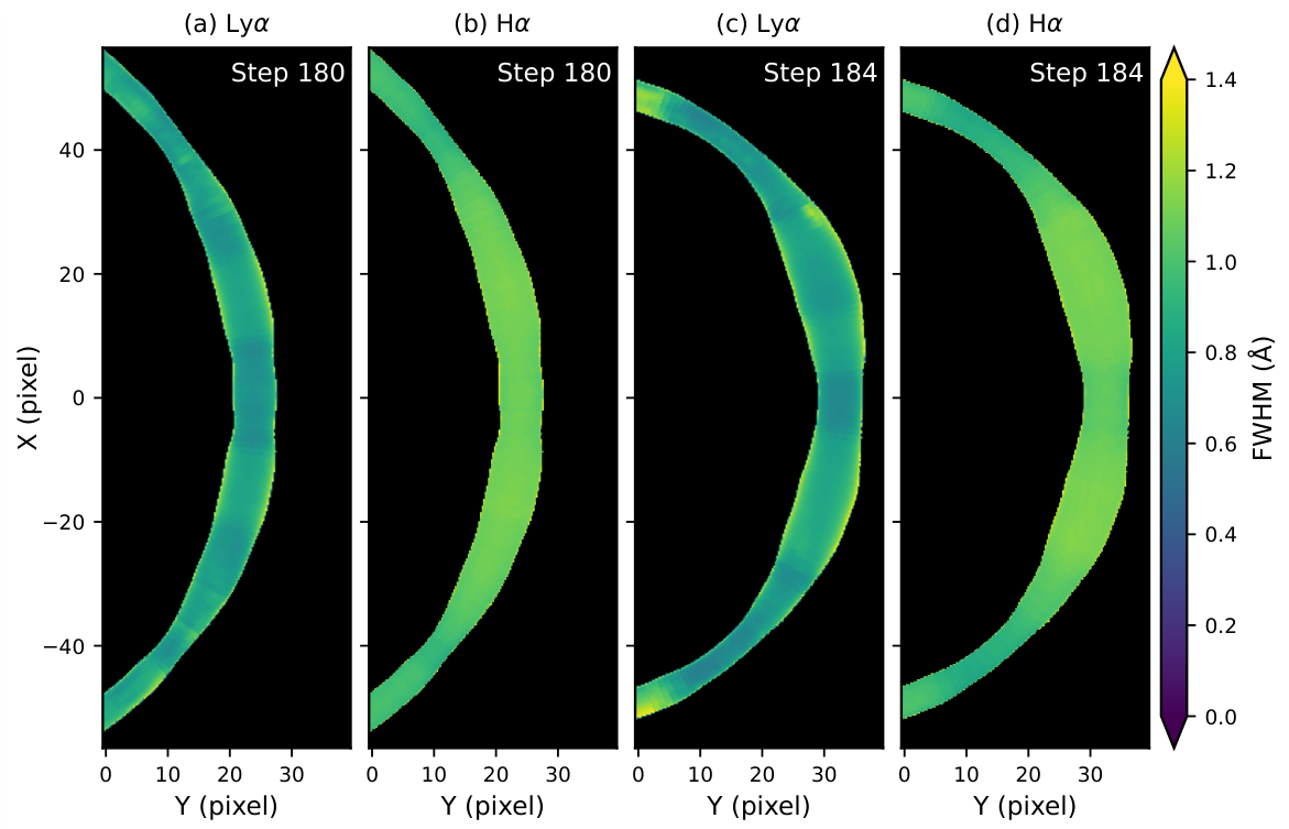
Figure 7.
Synthesized Lyα and Hα spectral properties together with cross-sectional 3D velocity fields for slice 62
at step 184. (a–b) Synthetic intensity images of Lyα and Hα, with the slice location marked by the white solid line.
(c–d) Synthetic stigmatic spectra along the slice (covering the prominence extent). (e–f) Synthetic Doppler velocity
maps. (g–i) Spatial distributions of the 3D velocity components (vx, vy, vz) across the cylindrical cross-section;
dotted circles indicate the outer boundary of the cylinder. Animated versions corresponding to steps 180 and 184
are available online.
Figure 7.
Synthesized Lyα and Hα spectral properties together with cross-sectional 3D velocity fields for slice 62
at step 184. (a–b) Synthetic intensity images of Lyα and Hα, with the slice location marked by the white solid line.
(c–d) Synthetic stigmatic spectra along the slice (covering the prominence extent). (e–f) Synthetic Doppler velocity
maps. (g–i) Spatial distributions of the 3D velocity components (vx, vy, vz) across the cylindrical cross-section;
dotted circles indicate the outer boundary of the cylinder. Animated versions corresponding to steps 180 and 184
are available online.
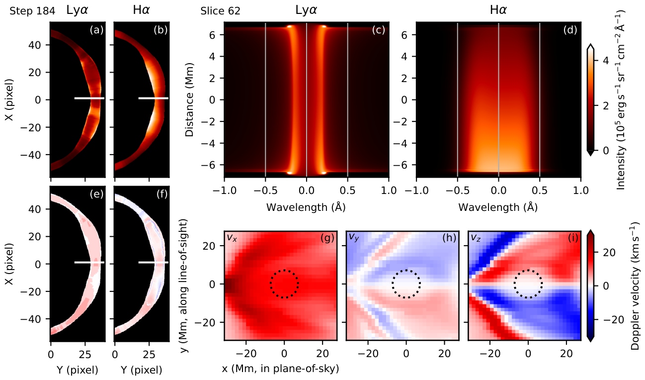
Figure 8.
Same as Figure 7, but for slice 75 at step 184.
Figure 8.
Same as Figure 7, but for slice 75 at step 184.
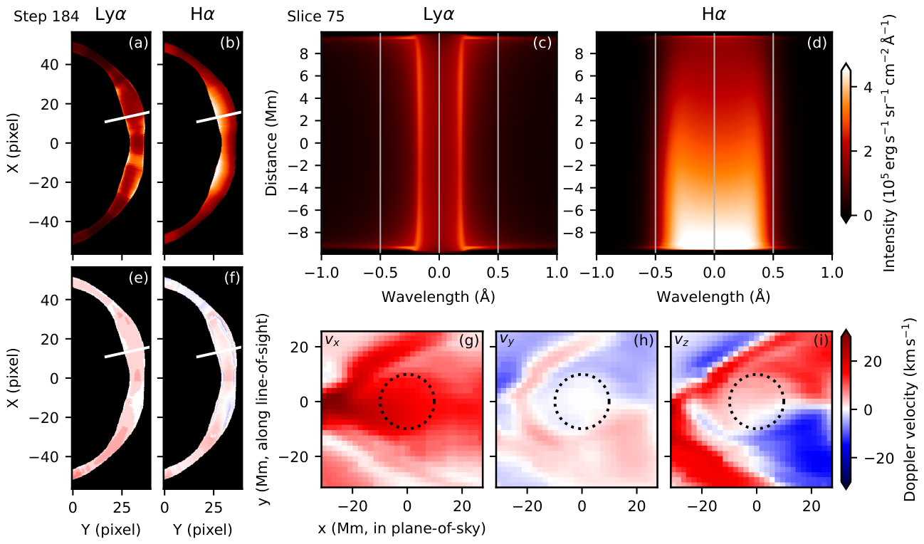
Figure 9.
Synthesized Lyα and Hα integrated line intensities computed for the static benchmark scenario at steps
180 and 184.
Figure 9.
Synthesized Lyα and Hα integrated line intensities computed for the static benchmark scenario at steps
180 and 184.
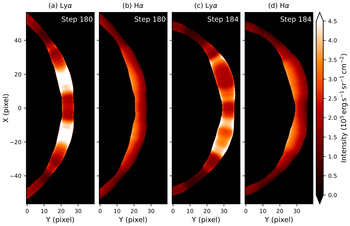
Figure 10.
Ratio of integrated line intensities between the dynamic scenario and the static benchmark for Ly and H at steps 180 and 184.
Figure 10.
Ratio of integrated line intensities between the dynamic scenario and the static benchmark for Ly and H at steps 180 and 184.
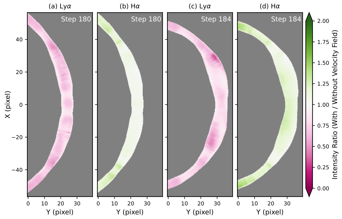
Figure 11.
Full-width-at-half-maximum (FWHM) distributions of Lyα and Hα computed for the static benchmark
scenario at steps 180 and 184.
Figure 11.
Full-width-at-half-maximum (FWHM) distributions of Lyα and Hα computed for the static benchmark
scenario at steps 180 and 184.
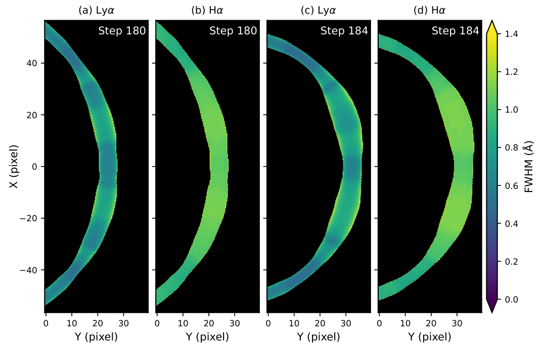
Figure 12.
Ratio of spectral line widths (FWHM) between the dynamic scenario and the static benchmark for Ly and H at steps 180 and 184.
Figure 12.
Ratio of spectral line widths (FWHM) between the dynamic scenario and the static benchmark for Ly and H at steps 180 and 184.
Disclaimer/Publisher’s Note: The statements, opinions and data contained in all publications are solely those of the individual author(s) and contributor(s) and not of MDPI and/or the editor(s). MDPI and/or the editor(s) disclaim responsibility for any injury to people or property resulting from any ideas, methods, instructions or products referred to in the content. |
© 2026 by the authors. Licensee MDPI, Basel, Switzerland. This article is an open access article distributed under the terms and conditions of the Creative Commons Attribution (CC BY) license (http://creativecommons.org/licenses/by/4.0/).
Copyright: This open access article is published under a Creative Commons CC BY 4.0 license, which permit the free download, distribution, and reuse, provided that the author and preprint are cited in any reuse.