

Submitted:
08 September 2026
Posted:
08 September 2026
You are already at the latest version
Abstract
Infrared thermography provides non-contact access to spatially resolved wall-temperature information, but large flow-boiling archives require traceable separation of physically meaningful variations from measurement artefacts. This study develops a physics-guided workflow for quality assessment of longitudinal infrared temperature profiles extracted from the central line of an externally observed heated foil in rectangular minichannels. The frozen dataset comprised 143,821 complete profiles, 35,666,447 spatial points, 447 source files, and 20 grid families. Leakage-safe source-file-level partitioning was used. Controlled evaluation covered eight local synthetic anomaly morphologies at three intensities and a separate global-offset challenge. A Random Forest using 64 engineered profile descriptors was compared with a five-channel masked residual one-dimensional convolutional neural network operating directly on complete profiles. On the locked test set, the Random Forest achieved an area under the precision-recall curve of 0.915, sensitivity of 0.731, and false-positive rate of 0.082, compared with 0.871, 0.452, and 0.063 for the neural model. Both models deteriorated under external grid-family transfer and remained near chance for uniform temperature offsets. The Random Forest is retained as the preferred supervised benchmark; geometry and grid-family transfer remain the principal unresolved limitation.
Keywords:
infrared thermography
; non-contact thermal diagnostics
; flow boiling
; minichannel
; temperature profile
; quality assessment
; anomaly detection
; Random Forest
; one-dimensional convolutional neural network
1. Introduction
Infrared thermography is widely used as a non-contact technique for observing temperature distributions on thermally loaded surfaces. In compact heat transfer systems, its value extends beyond qualitative imaging because spatially resolved surface-temperature data can serve as input to local heat-transfer reconstruction. The reliability of the derived quantities therefore depends on both the thermographic signal and the assumptions used to connect the externally observed surface to the fluid-side heat-transfer boundary.
This issue becomes critical in large experimental programmes. A single test may generate many spatially resolved temperature values, while hundreds of experiments can produce tens of millions of point-level records after spatial restructuring and merger with operating data. Manual inspection is then neither scalable nor reproducible. A simple outlier rule is also insufficient: a sharp local temperature change may represent a genuine thermal feature, an optical disturbance, a local emissivity problem, a missing-data segment, or instability introduced during downstream processing.
The present work addresses this problem for flow-boiling experiments in rectangular minichannels heated by a thin metal foil. Infrared measurements were acquired from the external side of the foil exposed to laboratory air. For database-scale processing, the full detector field was reduced to the central longitudinal line of the heated foil, thereby preserving the streamwise signal required for local thermal reconstruction while avoiding unnecessary propagation of the full two-dimensional image field.
Quantitative thermography requires a measurement model rather than image acquisition alone. Usamentiaga et al. [1] identified calibration, surface emissivity, and reflected apparent temperature among the principal influences on temperature accuracy, while also distinguishing passive temperature measurement from active thermographic non-destructive testing. Bagavathiappan et al. [2] reviewed infrared thermography as a non-contact, real-time condition-monitoring technique across electrical, mechanical, civil, and process applications, in which abnormal surface-temperature distributions are interpreted in relation to the inspected system. For convective heat-transfer measurements, Carlomagno and Cardone [3] showed that infrared thermography can provide non-intrusive, spatially resolved temperature and heat-flux information, but that sensor selection, calibration, and tangential conduction can constrain quantitative accuracy. Accordingly, the present longitudinal profiles cannot be treated as context-free numerical sequences: both their absolute level and their local gradients inherit radiometric, optical, and conduction-related assumptions.
Thermography has also been used to resolve spatial structure in boiling heat transfer. Kenning et al. [4] used liquid-crystal thermography to investigate local nucleate-boiling behaviour and highlighted both the spatial resolution offered by the method and the difficulty of interpreting interacting, orientation-dependent nucleation events. Liu and Pan [5] applied infrared thermography to a single rectangular microchannel and obtained transient outer-wall temperature fields and time-averaged local heat-transfer coefficients for two-phase boiling of water and ethanol. Korniliou et al. [6] combined infrared temperature measurement, high-speed flow visualisation, and pressure data in a polydimethylsiloxane (PDMS) microchannel; the resulting two-dimensional heat-transfer-coefficient maps were related to bubble nucleation, confinement, slug and annular structures, film thinning, and suspected dryout. These studies demonstrate that spatial non-uniformity can be physically informative rather than intrinsically anomalous.
In the authors' minichannel programme, Piasecka et al. [7] compared liquid-crystal and infrared thermography during FC-72 flow boiling and found broadly consistent temperature distributions and heat-transfer estimates, while retaining the complementary limitations of the two techniques. Subsequent work addressed the uncertainty and inverse-problem components of the measurement chain. Piasecka et al. [8] combined infrared thermography and fluid-temperature measurements with a two-dimensional Trefftz-based reconstruction and quantified uncertainty propagation, including a Monte Carlo assessment. Piasecka et al. [9] used Trefftz functions and ADINA calculations to recover local fluid-side heat-transfer coefficients from external wall-temperature measurements. These results make profile integrity consequential: a local artefact in the external temperature boundary can be propagated into reconstructed wall temperature, α and Nu.
Venegas et al. [10] combined infrared thermography of industrial equipment under normal and deliberately induced anomalous operating conditions with conventional machine learning and an augmented-reality maintenance interface. Their workflow illustrates how thermographic acquisition, preprocessing, and prediction can support inspection, but it addresses equipment-fault classification rather than flow-boiling profile quality. Willard et al. [11] organised physics-guided machine learning as a broader family of methods integrating scientific knowledge with data-driven models and hybrid physics-machine-learning frameworks. In the present study, physics-guided has the narrower operational meaning stated in Section 4: thermally interpretable descriptors, provenance, geometry-aware checks, and separation of measured from reconstructed quantities; the classifiers do not embed governing heat-transfer equations.
Method selection and evaluation design were chosen to match this bounded screening task. Breiman's Random Forest (RF) [12] provides a tree-ensemble representation that can use heterogeneous engineered descriptors and supports variable-importance inspection, whereas the survey by Kiranyaz et al. [13] shows the suitability of compact one-dimensional convolutional neural networks (1D CNNs) for ordered engineering signals while also noting the practical constraint of limited application-specific labelled data. Precision-recall curves are included because Saito and Rehmsmeier [14] demonstrated their value when class prevalence is asymmetric; here they are used as ranking diagnostics within a deliberately balanced 1:1 benchmark, not as estimates of operational positive predictive value. Kapoor and Narayanan [15] documented how leakage can inflate machine-learning results; this motivates source-file-level grouping before any fitting or threshold selection.
Recent reviews situate these choices within thermographic machine learning. He et al. [16] surveyed deep learning for infrared machine vision and thermography across passive and active applications, showing broad automation potential but heterogeneous data and deployment settings. Peng et al. [17] reviewed machine learning for thermographic non-destructive testing and identified limited dataset diversity and cross-condition generalisation as recurring constraints. Rosa et al. [18] showed in pulsed-thermography carbon-fibre-reinforced polymer (CFRP) segmentation that polynomial and derivative-based preprocessing materially improved U-Net results, illustrating that preprocessing choices can alter downstream performance rather than acting as a neutral preliminary step.
Anomaly detection adds a label problem. Pang et al. [19] described anomalies as rare and heterogeneous, which limits representative abnormal examples and complicates supervised evaluation. Peng et al. [20] proposed a training-free thermographic anomaly detector using random convolution kernels for image-based non-destructive testing. That contribution shows that supervised deep fitting is not the only route to thermographic anomaly screening, but it does not document a controlled synthetic-perturbation protocol equivalent to the one used here.
Liu et al. [21] reviewed unsupervised machine learning in active infrared thermography across six tasks: image denoising, non-uniform background removal, super-resolution enhancement, feature extraction, image segmentation, and depth prediction. They also identified limited labelled data, transferability and generalisation, and interpretability as continuing concerns, while noting the practical value of simpler traditional methods. Their review concerns principally active thermographic non-destructive testing rather than flow boiling; nevertheless, the methodological issues are directly relevant to quality assessment of thermographic profiles and to the present comparison between engineered and direct-profile models.
Reference [22] established the integrated database and reported a pilot point-level Random-Forest regression benchmark for reconstructed α and Nu. By contrast, the present article asks whether complete external temperature profiles can be screened before reconstruction. Its contributions are a frozen profile-level anomaly taxonomy, a comparison of a 64-descriptor RF and a direct-profile CNN, leakage-safe source-file-level evaluation, transfer testing across external grid families, and a separate global-offset boundary challenge. The classifiers use only measured-profile representations; α, Nu, and other downstream reconstructed quantities are not model inputs.
The present study focuses on profile-level quality assessment rather than on re-evaluating the physical effects of surface condition, module orientation, or mass flow rate, which require separate controlled matched comparisons. Its purpose is to develop and evaluate a traceable diagnostic framework that operates on the measured thermographic profile before that signal is used to reconstruct wall temperature, local heat transfer coefficient, and Nusselt number. Accordingly, the specific objectives are: (i) to document the central-line thermographic data structure and its provenance; (ii) to define deterministic and engineered profile descriptors linked to plausible anomaly morphologies; (iii) to establish a reproducible synthetic-anomaly benchmark in the absence of comprehensive real-error labels; (iv) to compare an interpretable RF with a direct-profile masked 1D CNN under leakage-safe source-file separation; and (v) to quantify performance loss under previously unseen grid-family and profile-length domains.
2. Experimental and Thermographic Measurement Framework
2.1. Rectangular Minichannel Test Sections
The experiments were conducted in a closed-loop flow-boiling facility comprising the working-fluid circuit, electrical power-supply and control systems, and synchronised thermal, hydraulic, and visual measurement systems. The working-fluid loop included a gear pump controlled by a variable-frequency drive, a pressure-stabilisation tank, a heat exchanger, and a Coriolis mass flowmeter. Fluid temperature and pressure were measured at the inlet and outlet of the test module. The heated wall was supplied electrically by direct resistive heating, while the principal thermal diagnostic was infrared measurement of the external, air-facing surface of the heated foil. In experimental campaigns incorporating simultaneous flow-pattern observation, a high-speed camera viewed the channels through the transparent wall on the opposite side of the module.
The rectangular-minichannel test section had a modular sandwich-type construction. A thin metallic heating foil made of Haynes-230 formed one wall of the parallel minichannels and was clamped between the structural elements of the module, while a transparent glass plate provided optical access to the flow on the opposite side. The foil was connected to copper electrodes and heated directly by Joule heating. In the representative 43-mm-long configuration, the individual minichannels were approximately 1 mm deep and 6 mm wide, and the heated foil was approximately 0.1 mm thick. Aluminium-alloy structural elements and polymeric spacers were used to define and seal the channel geometry. The infrared camera observed the external surface of the foil, whereas the working fluid contacted its opposite surface.
The integrated archive does not correspond to a single immutable test-section geometry. Successive experimental campaigns employed different numbers of parallel minichannels, surface preparations, module orientations, and selected geometric details while retaining the same general measurement concept. The configurations represented in Figure 1 should therefore be interpreted as members of a modular test-section family rather than repeated realisations of one nominal geometry. This distinction is important for the present study because changes in spatial discretisation and observation geometry are reflected in the profile grid families used for model development and transfer assessment.
The source data were obtained from a multi-campaign experimental programme involving rectangular minichannel modules operated with dielectric working fluids, different surface conditions, channel configurations, and spatial orientations. The heated wall was formed by a thin metal foil, while the opposite side of the channel was optically accessible for flow observation. Because the exact geometry varied among campaigns, geometry was retained as source-file-linked metadata rather than reduced to a single nominal configuration.
Across the archived campaigns, the test-section family included multiple channel-count variants, including configurations with 5–25 parallel rectangular minichannels. Channel width and depth, heated and infrared-observation lengths, foil thickness, hydraulic diameter, and surface preparation were campaign-specific. In the present article, these quantities are therefore retained as source-file-linked geometry descriptors and as defining attributes of the grid families rather than collapsed into one nominal test-section geometry.
2.2. Infrared Acquisition and Central-Line Extraction
The external surface temperature of the heated foil was measured by an infrared camera. The observed surface was the foil side facing the laboratory environment rather than the fluid-wetted side. The camera signal therefore provided a non-contact measurement of the externally visible foil temperature, which subsequently served as input to the local thermal reconstruction.
For the integrated profile database, the full two-dimensional thermogram was not propagated into every merged record. Instead, a central longitudinal line was extracted along the heated foil in the streamwise direction. Depending on the grid family, a complete profile contained between 73 and 434 ordered spatial points. This reduced representation preserved the profile shape used by the quality-assessment models and retained the link to the physical coordinate x.
For quantitative interpretation, the infrared camera configuration and radiometric settings form part of the measurement model [1,2,3]. Because the archive combines several experimental campaigns, campaign-dependent acquisition and radiometric settings should not be treated as a single invariant value. The principal camera specifications and the thermographic acquisition, radiometric, environmental, and profile-extraction settings relevant to the analysed 2021–2022 experimental series are summarised in Table 1.
The settings listed in Table 1 determine the radiometric comparability and spatial bandwidth of the extracted profiles. In particular, surface emissivity and the radiometric input parameters affect the absolute temperature level, whereas detector resolution, optical geometry, spatial calibration, and profile extraction affect local gradients, roughness, and the apparent morphology of short anomalies.
The experimental concept, the range of modular test-section geometries, and the relationship between the flow loop and infrared acquisition are summarised in Figure 1.
As shown in Figure 1, it can be observed that the experimental archive includes several channel-count configurations while retaining the same general measurement concept. The infrared camera observes the external, air-facing side of the electrically heated foil rather than the fluid-wetted surface. Consequently, the measured infrared-temperature profile constitutes an external thermal boundary signal and not the reconstructed fluid-side wall temperature itself. Maintaining the link between the measured TIR profile, its streamwise coordinate, the source-file provenance, and the corresponding module geometry is therefore essential for the subsequent foil-conduction reconstruction and for the grid-family-based analysis used in this study.
2.3. Measurement Traceability and Linked Operating Variables
Each thermographic profile remained linked to the experimental source file and to the variables required for reconstruction and contextual quality assessment. Table 2 summarises the principal data blocks retained in the integrated architecture.
Table 2 shows that thermography supplies the primary screening signal, whereas the electrical, boundary-condition, hydraulic, and metadata blocks preserve the experimental context required for interpretation. Reconstructed wall temperature, α, Nu, and regime or QC fields are downstream quantities and are not inputs to either supervised classifier.
The source file was retained as the primary provenance group because profiles originating from one experiment share geometry, boundary conditions, acquisition history, and data-processing lineage. This grouping was also used to prevent source-level information leakage during model development and final evaluation [15].
3. Data Architecture and Reconstruction of Longitudinal Temperature Profiles
3.1. Source-File-Level Data Organisation
The present analysis builds on the previously documented integrated rectangular-minichannel database, harmonisation workflow, and source-file-level quality-control architecture [22]. The complete provenance archive reported in Ref. [22] comprises 449 experimental source files. The profile-resolved Parquet layer available for the present analysis contained 447 source files; two catalogued 10-Hz series were not represented in this layer and were neither imputed nor replaced. Profile-level completeness filtering was subsequently applied within this 447-source population, yielding 143,821 complete physical profiles and 35,666,447 spatial points. The profiles were organised into 20 grid families defined by their physical coordinate grid and nominal number of points.
The source-file-level partition of the resulting complete-profile dataset, together with the analytical role assigned to each subset, is summarised in Table 3.
From the results presented in Table 3, it can be observed that the largest part of the complete-profile dataset was assigned to model fitting, whereas separate validation and locked test subsets were retained for model selection and final internal evaluation, respectively. These three subsets contain profiles from the same three grid families but originate from mutually exclusive source files. In contrast, the external-grid subset comprises 17 different grid families and was therefore reserved specifically for assessing transfer to profile geometries not represented during model development. This partitioning separates source-file generalisation within the internally represented geometries from the more demanding problem of transfer across spatial-grid configurations.
3.2. Reconstruction and Identity of Individual Line Profiles
An individual profile was represented by the unique identifier physical_profile_id and linked to source_file, grid_family_id, nominal_x_count, dataset_split, and the ordered coordinate x_m. Within a grid family, all profiles shared the same spatial coordinate vector. The unique profile identifier allowed the unmodified experimental profile, labelled clean in the benchmark, and its synthetically modified copy to be paired exactly during evaluation while retaining the original experimental provenance.
3.3. Separation of Measured, Derived, and Benchmark Signals
The primary measured signal used by both supervised models was the temperature recorded by the infrared camera on the outer surface of the heated foil. In the manuscript, this quantity is denoted as TIR, whereas the corresponding processed-data field is T_irt_C. This signal constituted the external infrared temperature profile. Synthetic anomalies were introduced only into a copy of T_irt_C; the frozen clean profile and the corresponding downstream arrays remained unchanged. This non-destructive architecture allows any flagged profile to be compared directly with the original measurement and, when necessary, reprocessed without compromising data provenance. In the benchmark terminology used below, clean denotes an unmodified experimental profile that passed the predefined completeness and integrity criteria and was not synthetically altered. This operational label does not imply expert-confirmed absence of every possible acquisition artefact.
The complete profile-screening and decision-support pathway is summarised in Figure 2.
Figure 2 shows that the supervised anomaly score is only one evidence layer. The raw profile and its provenance remain unchanged, and any correction, review, or rejection decision is separated from the downstream thermal reconstruction.
4. Physics-Guided Quality-Assessment Framework
Here, physics-guided refers to the use of thermally interpretable profile descriptors, experimental provenance, geometry-aware checks, and separation of measured and reconstructed quantities; the supervised classifiers themselves do not embed governing heat transfer equations.
4.1. Design Principles
The quality-assessment framework follows three principles. First, the raw measured profile and its provenance are preserved. Second, local smoothness alone cannot define validity because physically meaningful boiling-related structures may be spatially non-uniform. Third, any automated correction or exclusion must remain reversible and auditable. The present benchmark therefore classifies complete profiles as clean or synthetically anomalous; it does not automatically overwrite local temperatures.
4.2. Deterministic Integrity and Plausibility Checks
A deterministic audit layer checks missing values, duplicated or non-monotonic coordinates, incomplete profile keys, non-finite values, and inconsistent geometry. Missingness is retained explicitly because dropout segments form a physically distinct data-quality category and should not disappear through silent interpolation.
4.3. Profile-Level Robust Statistics and Shape Descriptors
The engineered representation combines thermal-level statistics with descriptors of global trend, first and second spatial differences, flatline persistence, spike residuals, profile roughness, multiscale step contrast, local drift, edge behaviour, and missingness. Geometry descriptors were retained for audit but excluded from the principal Random Forest so that the classifier could not identify anomalies merely by profile length or grid family.
4.4. Decision Support Rather than Automatic Denoising
The framework distinguishes four operational outcomes: retain, flag for review, flag for possible reversible correction, or reject from downstream reconstruction. The present study evaluates anomaly screening and review prioritisation; it does not benchmark an automatic temperature-correction algorithm. Table 4 summarises the evidence layers used in the decision process.
The optional post-reconstruction consistency layer is not an input to either supervised pre-screening classifier. When used, it is applied only after thermal reconstruction as an independent secondary QC check. No single evidence layer is sufficient to distinguish a true physical hot region from an acquisition artefact. The supervised score is therefore intended to prioritise profiles for review and to provide a reproducible benchmark of anomaly sensitivity.
5. Machine-Learning-Assisted Anomaly Detection
5.1. Frozen Synthetic-Anomaly Protocol
Comprehensive real-error labels were not available for the historical archive, which is consistent with the broader problem of rare, heterogeneous, and incompletely labelled anomalies [19,21]. Controlled sensitivity was therefore evaluated using a frozen deterministic synthetic-anomaly protocol developed for the present profile-level benchmark. Each clean physical profile was paired with one modified copy assigned to one anomaly type and one intensity. Eight anomaly morphologies formed the primary benchmark, while a spatially uniform global temperature offset was reserved as an out-of-taxonomy challenge. The operations are reproducible test perturbations and are not intended as complete physical simulations of camera, radiometric, or acquisition errors. Table 5 summarises the protocol.
Perturbation magnitudes were defined relative to two robust scales calculated separately for each clean infrared-temperature profile. For a profile TIR, the point-to-point scale was defined using the median absolute deviation (MAD) as
and the robust profile range as
RT = max(P95(TIR) − P5(TIR), 1.0 °C),
For signed perturbations, the applied amplitude was
A = max(kΔsΔT, kRRT, Amin).
For isolated spikes, (kΔ, kR, Amin) was (4.0, 0.020, 0.40 °C), (7.0, 0.050, 0.80 °C), and (10.0, 0.100, 1.50 °C) at low, medium, and high intensity, respectively, with corresponding widths of 1, 2, and 3 adjacent points. For local steps, the respective settings were (2.5, 0.015, 0.30 °C), (4.5, 0.040, 0.70 °C), and (7.0, 0.080, 1.40 °C), applied over 0.04, 0.08, and 0.15 of the profile length. Local linear drift used (2.5, 0.020, 0.30 °C), (4.5, 0.050, 0.75 °C), and (7.0, 0.100, 1.50 °C), over fractions 0.30, 0.50, and 0.70 of the profile length. The separate global-offset challenge used (1.5, 0.010, 0.25 °C), (3.0, 0.030, 0.75 °C), and (5.0, 0.060, 1.50 °C) over the complete profile.
Noise bursts consisted of zero-mean Gaussian noise with standard deviation 2sΔT, 4sΔT, or 7sΔT, applied over 0.06, 0.12, or 0.20 of the profile length for low, medium, and high intensity, respectively. Flatline segments replaced fractions 0.04, 0.08, or 0.15 of the profile by the first value of the selected segment, whereas dropout segments replaced fractions 0.02, 0.05, or 0.10 by missing values. Local smoothing was applied over profile fractions 0.15, 0.25, or 0.40 using moving-average window fractions 0.03, 0.07, or 0.15, respectively. Spatial-shift anomalies displaced the complete profile by 0.01, 0.03, or 0.06 of its length; the displacement was rounded to an integer number of points, with a minimum of one point, and the newly exposed edge was filled with the nearest endpoint value.
Fractional segment widths were converted to integer point counts by rounding and were constrained to minimum widths of 2 points for local steps, 3 points for noise bursts and flatlines, 1 point for dropout, and 5 points for local smoothing and linear drift. The smoothing window had a minimum of 3 points, was limited to the selected segment length, and was reduced by one point when necessary to obtain an odd window; moving-average filtering used edge-value padding. Local perturbations were positioned pseudo-randomly but reproducibly while preserving an interior margin of max[3, ⌈0.05N⌉] points whenever geometrically possible; otherwise, all geometrically valid starting positions were admissible.
Positive and negative directions were balanced for isolated spikes, local steps, linear drifts, and global offsets, while spatial shifts were balanced between the two streamwise directions. Randomness was frozen using a master seed of 20260719 and split-specific seeds of 20260719, 20260720, 20260721, and 20260722 for the training, validation, test, and external-grid partitions, respectively. For each corrupted profile, the pseudo-random generator was derived as SeedSequence([split_seed, physical_profile_id, anomaly_code, intensity_code, replicate_id]). Only one anomaly was applied to each corrupted profile.
An anomaly assignment was considered effective only when at least one value remained changed after conversion to the persisted float32 representation. For initially zero-effect flatline and local-smoothing assignments, the original frozen position was retained whenever it produced a non-zero change; otherwise, all admissible positions were examined and the position changing the greatest number of float32 points was selected deterministically. Total absolute temperature change was used as the secondary criterion and the earliest position resolved an exact tie. When no effective placement existed, and for zero-effect spatial-shift assignments, the complete anomaly assignment was deterministically exchanged with a feasible donor assignment within the same dataset split. Donors from the same grid family were prioritised, while profile identity, source-file provenance, experimental metadata, and the frozen setting and direction counts were preserved. The repaired benchmark was then exhaustively preflighted over all 143,821 primary profiles with no failures.
This construction preserved the frozen morphology and intensity balance while making the synthetic benchmark reproducible across all 20 grid families.
Representative examples of the clean reference profile and the corresponding synthetically modified profiles are presented in Figure 3. The purpose of this comparison is to illustrate the distinct signal properties affected by the frozen benchmark operations rather than to reproduce specific physical camera failures. The selected morphologies span local amplitude disturbances, increased or suppressed short-scale variability, local changes in level or trend, missing-data regions, spatial displacement, and a uniform change in absolute temperature level. Presenting the anomalies against the same underlying profile makes it possible to distinguish changes in local morphology from changes that preserve the overall profile shape. This distinction is relevant to the subsequent comparison of engineered descriptors and the direct-profile CNN, because the two model classes receive substantially different representations of these signal modifications.
When analysing Figure 3, it can be observed that the benchmark operations affect qualitatively different properties of the temperature profile. The isolated spike and noise-burst cases introduce local high-frequency departures while largely preserving the underlying large-scale temperature trend. In contrast, the flatline and local-smoothing operations suppress existing spatial variation, although in different ways: the flatline imposes an artificial constant segment, whereas smoothing reduces local detail without creating a strictly constant region. The local-step and linear-drift cases modify the profile level or trend over a finite streamwise interval and therefore produce broader deviations than the spike-type disturbances. Spatial shift preserves much of the profile morphology but displaces characteristic features along the coordinate axis, while the dropout case removes information altogether rather than replacing it with a plausible temperature value.
The global-offset challenge is qualitatively different from the eight primary anomalies. It changes the absolute temperature level while leaving the local shape, gradients, and relative spatial structure essentially unchanged. This makes it a useful boundary test for determining whether the classifiers respond to generic thermographic invalidity or principally to the local morphological changes represented during training. Figure 3 therefore illustrates why no single smoothness or amplitude criterion can represent the complete benchmark and provides the physical motivation for combining thermal-level, difference-based, roughness, missingness, step, drift, and spatial descriptors in the engineered representation considered in Section 5.2.
5.2. Engineered-Feature Random Forest
The feature extractor produced 70 descriptors in ten groups. Four geometry descriptors were retained for audit only, and two edge-missingness indicators were exact constants in the final benchmark. The Random Forest therefore used 64 features: four missingness variables after constant removal, 13 thermal-level descriptors, seven global-shape descriptors, ten first-difference descriptors, five second-difference descriptors, four flatline descriptors, ten spike/roughness descriptors, six multiscale-step descriptors, and five local-drift/edge descriptors. Random Forests were used as the interpretable tree-ensemble benchmark [12].
The complete frozen 64-feature manifest, including descriptor definitions, units or normalisation, window rules, and missing-value handling, will be made available in the GitHub repository “boiling-heat-transfer-minichannel” upon publication. No external standardisation or feature scaling was applied before Random-Forest fitting; the engineered descriptors were passed directly to the classifier as float32 values. Normalisation was intrinsic only to descriptors explicitly defined in normalised form, including quantities divided by the robust temperature range and spatial positions expressed on the normalised profile coordinate. Missingness descriptors were calculated before interpolation. Non-finite temperature values were subsequently interpolated along the physical xm coordinate before calculation of the remaining thermal and morphological descriptors. The two edge-missingness indicators, nan_at_left_edge and nan_at_right_edge, were exact constants in the frozen benchmark and were therefore excluded from the final 64-feature model input.
Three Random Forest candidates were fitted to 93,109 clean and 93,109 synthetic training profiles. Candidate RF_depth18_leaf5_sqrt used 300 trees, a maximum depth of 18, a minimum leaf size of 5, max_features = sqrt, max_samples = 0.80, and random_state = 20260719. Candidate RF_depth26_leaf2_sqrt used 300 trees, a maximum depth of 26, a minimum leaf size of 2, max_features = sqrt, max_samples = 0.80, and random_state = 20260720. Candidate RF_depth22_leaf2_wide used 240 trees, a maximum depth of 22, a minimum leaf size of 2, max_features = 0.50, max_samples = 0.75, and random_state = 20260721. All candidates used the Gini criterion, min_samples_split = 2, bootstrap sampling, and no class weighting. Selection prioritised sensitivity at a target validation clean-profile false-positive rate (FPR) of 1%, followed by area under the precision-recall curve (AUPRC) and area under the receiver operating characteristic curve (AUROC). The RF_depth22_leaf2_wide configuration was selected and its threshold was frozen at 0.68350612 using clean validation profiles. On the complete paired validation set it achieved sensitivity 0.712, FPR 0.00998, AUROC 0.927, and AUPRC 0.947.
5.3. Five-Channel Masked Residual 1D CNN
The five-channel input comprised standardised absolute temperature (temperature_absolute), standardised profile-centred temperature shape (temperature_centered_shape), scaled spatial coordinate (x_coordinate), a physical-geometry mask (geometry_valid_mask), and an observed-temperature mask (temperature_observed_mask). Profiles were right-padded to 448 points without interpolation or resampling to a common spatial grid. The network began with a bias-free 1D convolution mapping the five input channels to 64 channels using a kernel size of 9, followed by GroupNorm with eight groups and Gaussian error linear unit (GELU) activation. Four masked residual blocks subsequently expanded the representation to 96, 160, 256, and 256 channels, with strides of 2, 2, 2, and 1, respectively. Each block contained bias-free convolutions with kernel sizes of 7 and 5, GroupNorm with eight groups, GELU activation, and dropout rates of 0.05, 0.05, 0.10, and 0.10 in successive blocks; a bias-free 1 × 1 shortcut convolution was used whenever the channel count or stride changed. The geometry mask was reapplied after the stem and propagated through the residual blocks by nearest-neighbour resizing to each block output; it was reapplied after residual addition and activation, preventing padded positions from contributing to the learned representation. Masked global mean and maximum pooling were concatenated and passed through a 512–192–1 classification head with GELU activation and dropout 0.20. The resulting network contained 1,892,673 trainable parameters.
The CNN was optimised with BCEWithLogitsLoss and AdamW using an initial learning rate of 2 × 10⁻⁴, weight decay of 1 × 10⁻⁴, and a batch size of 1024. ReduceLROnPlateau halved the learning rate after one epoch without an absolute validation-AUPRC improvement of at least 1 × 10⁻⁴, with a minimum learning rate of 2 × 10⁻⁵; gradient norms were clipped at 5.0. Training used seed 20260723 and was limited to 12 epochs, with early-stopping patience of four epochs and the same minimum validation-AUPRC improvement of 1 × 10⁻⁴. The best checkpoint occurred at epoch 12. The frozen encoder standardised only finite observed temperatures. For the centred-shape channel, each profile mean was first calculated from its finite observed points and subtracted before application of the frozen shape centre and scale. Missing in-profile temperature positions and right-padding positions were encoded as zero in both temperature channels, and the observed-temperature and geometry masks distinguished them. The frozen temperature-channel normalisation statistics were fitted exclusively on the 93,109 clean training profiles, comprising 23,405,210 observed temperature points from grid families 8, 9, and 19; no validation, test, or external-grid profile contributed to normalisation fitting. Training used 186,218 paired rows and validation used 42,286 paired rows on an NVIDIA A100 with brain floating-point 16-bit (BF16) arithmetic. The frozen threshold of 0.99998927 was selected from clean validation profiles at an FPR of 0.00974; validation sensitivity, AUROC, and AUPRC were 0.418, 0.872, and 0.895, respectively. No test, external-grid, or challenge result was used for architecture selection or threshold calibration.
5.4. Leakage-Safe and Locked Evaluation
All partitions were defined at source-file level. Clean and synthetic copies of a physical profile remained in the same split and were paired by physical_profile_id. Test and external-grid evaluations were opened once after model and threshold selection and were then locked. Ranking metrics and receiver operating characteristic (ROC)/precision-recall curves were reconstructed from persisted profile-level scores. Threshold-dependent counts and derived metrics were taken from the locked summary tables because finite-precision serialization of scores and thresholds can move a small number of observations located exactly at the operating boundary. The source-file grouping and locked-evaluation procedure were adopted specifically to prevent leakage-driven optimism [15].
The leakage-safe development and locked-evaluation sequence is summarised in Figure 4.
Figure 4 makes explicit that source-file grouping precedes model fitting and that the validation partition is the only partition used for model and threshold selection. The test and external-grid results therefore quantify generalisation without post hoc threshold adaptation.
6. Computational Implementation
The complete dataset was stored in columnar Parquet and family-specific array formats. Processing used column projection, predicate filtering, grouped scans, and versioned intermediate outputs rather than manual full-table opening. Feature extraction and Random Forest fitting were performed in Python using NumPy, pandas, PyArrow, and scikit-learn. The masked CNN was implemented in PyTorch. The available computing environment provided approximately 47 central processing unit (CPU) cores, 256 GB of random-access memory (RAM), and an NVIDIA A100 80 GB graphics processing unit (GPU).
The frozen computational environment used Python 3.12.6 with NumPy 2.4.4, pandas 3.0.2, and PyTorch 2.11.0+cu130 with CUDA 13.0 and cuDNN 9.19.0. CNN computations were performed on an NVIDIA A100 80 GB PCIe GPU using BF16 arithmetic.
Table 6 gives the final supervised model configurations. The result-synthesis stage did not retrain either model, rerun inference, or recalibrate thresholds; it only aligned the frozen score files, reconstructed ranking metrics, prepared publication tables, and generated figures.
When analysing the configurations in Table 6, it can be observed that the comparison contrasts an explicitly engineered 64-descriptor representation with a substantially larger direct-profile model while retaining validation-locked thresholds. The parameter counts and thresholds describe the frozen implementations; they should not be interpreted as evidence that greater model complexity should provide better screening performance.
The locked score table for each supervised model contained 160,562 evaluated rows: 39,066 primary-test rows and 20,072 primary external-grid rows, together with 42,286 global-offset-challenge validation rows, 39,066 challenge-test rows, and 20,072 challenge external-grid rows. Primary validation scores had already been fixed during model and threshold selection and were not included in this final scoring stage. Profile identifiers were exactly aligned between the final RF and CNN score tables, and all computational artefacts were versioned and validated with Secure Hash Algorithm 256-bit (SHA256) checksums.
7. Results
7.1. Profile Coverage and Benchmark Integrity
The analysis covered all 143,821 complete profiles, 20 grid families, and 447 source files. The paired primary evaluation contained 42,286 validation rows, 39,066 test rows, and 20,072 external-grid rows per model, with equal numbers of clean and synthetic profiles in each group. The global-offset challenge was evaluated on the same three split sizes. Challenge validation was diagnostic only and did not alter model or threshold selection. Generator and feature-extraction audits reported no remaining zero-effect primary anomalies, and the RF and CNN evaluation tables contained identical physical-profile keys.
The internal test set contained three grid families with nominal lengths of 116 and 434 points. The external-grid set contained 17 different families with nominal lengths from 73 to 433 points. Consequently, the external partition tested both source-file separation and a substantial geometry shift.
7.2. Aggregate Random Forest and CNN Performance
The locked aggregate performance of the two supervised models is summarised in Table 7. The operating thresholds were fixed from validation and were not adapted to either the test or external-grid partitions.
When analysing the results presented in Table 7, it can be observed that the Random Forest provided stronger locked test-set ranking and detection performance. The differences reported below were calculated from the unrounded frozen metrics. Its AUPRC and AUROC exceeded the CNN values by 0.044 and 0.041, respectively, and its sensitivity was higher by 0.279. The CNN reduced the FPR by only 0.020 at its validation-selected threshold. The corresponding frozen F1 scores (harmonic mean of precision and recall) were 0.806 for the Random Forest and 0.597 for the CNN. On the external-grid set, the Random Forest retained higher ranking quality and sensitivity, but its FPR increased to 0.487. The CNN produced fewer external false positives, yet its sensitivity fell to 0.537 and its AUPRC to 0.738. Thus, neither frozen threshold was fully portable across unseen grid families, and the result favours the Random Forest only within the present feature set, anomaly taxonomy, and evaluation domains.
The corresponding ROC and precision-recall curves are presented in Figure 5. The figure combines the locked test and external-grid evaluations so that discrimination and transfer loss can be inspected directly.
When analysing the curves presented in Figure 5, the Random-Forest advantage can be observed across the threshold-independent ranking curves and is therefore not restricted to the selected operating threshold. Both models lost discrimination under external-grid transfer, with the reduction being more pronounced for the CNN. The curves and the locked operating-point results in Table 7 provide complementary evidence: the former characterise ranking across possible thresholds, whereas the latter describe performance only at the preselected thresholds. The balanced paired design gives a precision-recall baseline of 0.5, and both models remained above this baseline for the primary benchmark. Precision-recall interpretation follows the recommendations for classifier assessment under class imbalance [14]. Because the benchmark was deliberately balanced, AUPRC and precision characterise discrimination under the defined evaluation protocol and must not be interpreted as estimates of operational positive predictive value in the historical archive, where the true anomaly prevalence is unknown.
7.3. Sensitivity by Anomaly Morphology
Aggregate sensitivity can obscure whether a classifier detects the same anomaly morphologies. Table 8 therefore reports profile-weighted sensitivity for each primary anomaly type, separately for the test and external-grid sets.
When analysing the results presented in Table 8, it can be observed that dropout segments were detected almost perfectly by both models. The Random Forest also detected all test flatline profiles and showed high sensitivity to spatial shifts and noise bursts. The CNN slightly exceeded the Random Forest only for local steps on the test set (0.523 versus 0.522), while dropout sensitivity was nearly identical (0.997 versus 1.000). The largest test-set differences occurred for spatial shift, flatline, local smoothing, and noise burst. On the external-grid set, the Random Forest was more sensitive for all eight anomaly morphologies. The aggregate performance difference therefore reflects a morphology-dependent response rather than a uniform displacement between the two classifiers.
Figure 6 visualises these morphology-dependent differences. The two panels use the same scale, allowing the internal and external results to be compared without rescaling.
As can be observed in Figure 6, the differences become most pronounced for spatial shift, flatline, local smoothing, and noise burst, whereas local-step sensitivity is almost identical on the test set. Flatline persistence, second differences, roughness, missingness, and spatial-shift-related structure are represented explicitly in the Random-Forest feature set. This correspondence may contribute to the stronger Random-Forest response, although the present benchmark did not perform a causal feature-attribution analysis. The external-grid panel further indicates that the engineered response transferred more consistently across the evaluated morphologies than the representation learned by the direct-profile CNN.
7.4. Effect of Anomaly Intensity
When analysing sensitivity by anomaly intensity, a consistent increase can be observed for both models and both evaluation domains. On the test set, Random-Forest sensitivity increased from 0.439 for low-intensity anomalies to 0.806 for medium intensity and 0.949 for high intensity; the corresponding CNN values were 0.209, 0.453, and 0.695. On the external-grid set, the Random Forest reached 0.681, 0.900, and 0.983, while the CNN reached 0.364, 0.537, and 0.711. Weak perturbations were therefore the most difficult part of the controlled benchmark, but the CNN deficit persisted at every intensity and was not confined to the low-intensity category. Because intensity was defined by the frozen synthetic generator, these values characterise benchmark sensitivity and do not establish a physical camera-detection limit.
7.5. Geometry Transfer and Out-of-Taxonomy Challenge
The direct-profile CNN transfer results were further grouped by external profile-length class in Table 9. This grouping exposes a domain-dependent result that is not visible in the aggregate external metrics, while the family-level view in Figure 7 tests whether profile length alone is an adequate explanation.
When analysing the data presented in Table 9, short external profiles of 73-84 points had the weakest CNN ranking quality (AUPRC 0.660) and the highest grouped FPR (0.443). Intermediate profiles of 117-120 points had AUPRC 0.759, sensitivity 0.470, and FPR 0.139. Long profiles of 425-433 points achieved AUPRC 0.922 and zero false positives at the frozen threshold, although sensitivity remained 0.453. These grouped results do not define a simple monotonic relationship between profile length and performance. Within the internal test set, grid family 8 generated 1,226 of 1,228 CNN false positives, corresponding to 99.8% of all test false alarms. The false-positive burden was therefore strongly domain-specific rather than uniformly distributed across the test families.
Figure 7 relates length-group and family-level metrics to the nominal number of profile points. Selected family labels identify the principal diagnostic and extreme cases.
As shown in Figure 7, the family-level points do not follow a single monotonic performance curve with nominal profile length. Profile length is therefore an incomplete proxy for the domain shift: grid-family-specific geometry and associated score-distribution changes are also relevant. The observed clustering supports geometry-aware calibration or representation development across a broader family set before any increase in neural-network capacity is considered.
Figure 8 brings together two complementary boundary tests. Panel (a) shows the progressive sensitivity increase with synthetic-anomaly intensity, whereas panel (b) presents the separate global-offset challenge. The challenge was never used for training or threshold selection and tested whether classifiers trained on local morphology changes had acquired a generic response to absolute temperature displacement.
When analysing Figure 8b, both models remained approximately at chance for the global-offset challenge. The maximum absolute AUROC deviation from 0.5 across models and splits was 0.019, and anomaly and clean positive rates remained nearly equal at the frozen thresholds. Because a uniform offset changes the absolute temperature level without changing local profile shape, this near-chance result defines an application boundary: the present classifiers are detectors of the benchmarked local morphologies, not general thermographic-validity detectors. Global temperature-level errors therefore require independent calibration or reference-temperature checks; automatic temperature correction was not benchmarked.
8. Discussion
The principal result is that an engineered-feature Random Forest outperformed a substantially more complex direct-profile CNN under the same leakage-safe split and synthetic-anomaly protocol. This finding does not imply that convolutional models are intrinsically unsuitable for thermographic profiles. One-dimensional CNNs remain well suited to ordered engineering signals [13], but their performance depends on the available labelled domain and the representation learned from it. For the present training families and anomaly taxonomy, explicit descriptors of missingness, flatline persistence, spatial differences, roughness, step contrast, drift, and edge behaviour provided a more effective and transferable representation. This result is consistent with the practical role of heterogeneous engineered variables in Random Forests [12] and with Liu et al.'s observation that simpler traditional machine-learning methods remain valuable when interpretability and limited labelled data are important [21].
The operating-point comparison also requires nuance. The CNN produced a lower FPR than the Random Forest on both locked evaluation sets, but this reduction was accompanied by markedly lower sensitivity. On the test set, the FPR advantage was only 0.020 while sensitivity decreased by 0.279. On the external-grid set, the CNN reduced the FPR by 0.230 but sensitivity decreased by 0.318 and AUPRC by 0.092. The CNN therefore did not provide the preferable sensitivity-FPR trade-off at the frozen validation-selected threshold. These precision and AUPRC results describe the balanced benchmark and not real-world positive predictive value.
The external-grid results expose the main scientific limitation of the present models: domain transfer. The Random Forest retained high external sensitivity but generated many clean false positives, whereas the CNN showed strong family-specific score shifts and lower anomaly sensitivity. Family 8 dominated CNN false positives on the internal test set, while the external length-group pattern was not monotonic at family level. A single global threshold was therefore not portable across all grid geometries represented in the historical archive. Such domain sensitivity agrees with thermographic-machine-learning reviews that identify restricted dataset diversity, acquisition variability, and inspection-specific conditions as obstacles to robustness and generalisation [16,17,21].
Data quality and preprocessing must also be interpreted within the thermographic measurement chain. Quantitative temperature accuracy depends on calibration, emissivity, reflected radiation, spatial response, and conduction assumptions [1,2,3]. In a different active-thermography application, Rosa et al. [18] demonstrated that polynomial and derivative preprocessing materially changed CFRP segmentation performance. The present workflow therefore preserves the measured profile and records each deterministic or supervised operation rather than treating preprocessing as an invisible transformation. The result is a screening and review-prioritisation layer, not an automatic denoising or correction system.
The absence of comprehensive expert-confirmed error labels is consistent with the general anomaly-detection problem described by Pang et al. [19] and with the labelled-data limitations discussed for active thermography by Liu et al. [21]. The frozen synthetic operations provide controlled and repeatable sensitivity comparisons, but they cannot reproduce the full physical diversity or prevalence of camera, radiometric, acquisition, and processing errors. Peng et al. [20] addressed a related image-based thermographic non-destructive testing problem with a training-free random-convolution approach. That work illustrates a lightweight alternative to supervised deep fitting, but its task and data representation do not provide a direct performance comparator for the present profile-level synthetic benchmark.
The global-offset challenge supplies a complementary failure boundary. Both models were trained on local morphology anomalies and remained near chance when the complete profile was shifted uniformly. Neither model should therefore be regarded as a general-purpose thermographic validity detector. A global offset requires independent calibration checks or reference-temperature comparison, and the present study provides no evidence for automatic correction of such an error.
The practical value of the workflow lies in traceability and controlled failure analysis. The system preserves the measured profile, records the source file and grid family, quantifies which benchmark morphologies are detectable, and identifies domains in which the threshold is unreliable. This use as human-supervised decision support is aligned with quantitative thermography, automated inspection, and scientific-knowledge-guided machine-learning principles [1,2,10,11].
9. Limitations
Several limitations must be stated explicitly. First, the analysis uses a central longitudinal line rather than the complete two-dimensional thermographic field, so lateral artefacts and asymmetries are not represented. Second, the camera observes the external side of the heated foil; fluid-side thermal quantities depend on a separate reconstruction model. Third, the historical archive contains heterogeneous campaigns, fluids, surfaces, orientations, and module geometries. Although explicit geometry descriptors were excluded from the Random Forest, the CNN required a spatial-coordinate channel and geometry mask to distinguish physical from padded positions. These inputs can indirectly encode profile length and therefore constitute a potential source of grid-family-specific representation shift. Fourth, the supervised labels are controlled synthetic anomalies rather than comprehensive expert-confirmed real artefacts [19,21]. Controlled perturbations provide a reproducible sensitivity benchmark, but they do not constitute a complete physical model of radiometric or acquisition errors. The benchmark evaluates sensitivity to predefined profile operations but cannot establish the prevalence, morphology, or physical cause of artefacts occurring in the experimental archive. Only one anomaly was assigned to each synthetic profile, so compound anomalies and interactions among error mechanisms were not tested. Fifth, profile-level classification does not localise every affected point or determine the appropriate correction.
Finally, both thresholds were calibrated on internal validation families and were not portable across all test and external domains. The global-offset challenge also remained unresolved. Further development should therefore use train and validation data only, predeclare any new architecture or domain-calibration strategy, and reserve another untouched final evaluation rather than tuning against the already opened test and external-grid results.
10. Conclusions
A traceable machine-learning-assisted workflow was established for quality assessment of central-line infrared temperature profiles used in flow-boiling minichannel diagnostics. The principal conclusions are as follows:
- The frozen dataset comprised 143,821 complete profiles, 35,666,447 spatial points, 447 source files, and 20 grid families. Source-file-level partitioning prevented overlap of experimental source files among dataset partitions.
- The controlled benchmark covered eight local anomaly morphologies at three intensities and a separate global-offset challenge. Unmodified experimental profiles were preserved and all synthetic modifications remained reproducible and auditable.
- The 64-feature Random Forest was the preferred supervised benchmark. On the locked test set it achieved AUPRC 0.915 and sensitivity 0.731 at FPR 0.082, exceeding the masked 1D CNN in ranking quality and anomaly sensitivity.
- The CNN provided no overall advantage for the present screening objective despite operating directly on five-channel complete profiles. Its main relative benefit was a lower FPR, but this was obtained at a substantial sensitivity cost.
- Anomaly morphology strongly affected detectability. Dropout segments were detected almost perfectly by both models, whereas the CNN was weak for spatial shifts, local smoothing, flatline segments, and noise bursts. Local steps were the only test morphology for which CNN sensitivity was not lower than Random-Forest sensitivity.
- Geometry and grid-family transfer was the dominant unresolved limitation. Family 8 accounted for 99.8% of CNN test false positives, and external CNN performance differed sharply between short and long profile classes.
- Neither model reliably detected a uniform global temperature offset. Independent calibration checks, reference-temperature comparisons, or a specifically trained global-offset detector would be needed to address this failure mode.
The practical recommendation is to retain the engineered-feature Random Forest as the primary profile-screening model, use its output as decision support rather than automatic correction, and treat grid-family-specific score drift as an explicit calibration problem in future development.
Author Contributions
Conceptualization, M.P.; methodology, M.P.; software, M.P.; investigation, M.P. and A.P.; data curation, M.P.; formal analysis, M.P.; validation, M.P. and A.P.; visualization, A.P.; resources, M.P.; writing—original draft preparation, M.P. and A.P.; writing—review and editing, M.P. and A.P.; supervision, M.P.; project administration, M.P.; funding acquisition, M.P. All authors have read and agreed to the published version of the manuscript.
Funding
This research was funded by the National Science Centre, Poland, grant no. UMO-2025/57/B/ST8/00907. For the purpose of Open Access, the authors have applied a CC BY public copyright licence to the Author Accepted Manuscript (AAM) version arising from this submission.
Institutional Review Board Statement
Not applicable.
Informed Consent Statement
Not applicable.
Data Availability Statement
A representative processed data sample and basic documentation will be made publicly available in the GitHub repository “boiling-heat-transfer-minichannel” at https://github.com/MagdalenaPiasecka/boiling-heat-transfer-minichannel upon publication. The complete experimental datasets, source-file-level metadata, analysis code, and integrated Parquet database are archived in the PRACE-LAB data-storage infrastructure at Kielce University of Technology and are available from the corresponding author upon reasonable request.
Conflicts of Interest
The authors declare no conflicts of interest.
Nomenclature
| Symbols | |
| α | Local heat-transfer coefficient; W m⁻² K⁻¹ |
| A | Applied signed perturbation amplitude; °C |
| Amin | Minimum perturbation amplitude; °C |
| kΔ | Point-to-point-scale amplitude coefficient; – |
| kR | Robust-range amplitude coefficient; – |
| N | Number of spatial points in a profile; – |
| Nu | Nusselt number; – |
| P5 | Fifth-percentile operator |
| P95 | Ninety-fifth-percentile operator |
| RT | Robust profile range; °C |
| sΔT | Robust point-to-point temperature scale; °C |
| TIR | Temperature measured by the infrared camera on the outer surface of the heated foil; °C |
| Twall | Reconstructed wall temperature on the fluid side; °C |
| x | Streamwise coordinate; m |
| xm | Streamwise coordinate stored in metres for an ordered profile point; m |
| ΔTIR | First difference of adjacent infrared-temperature values; °C |
| Abbreviations | |
| 1D | One-dimensional |
| AUPRC | Area under the precision-recall curve |
| AUROC | Area under the receiver operating characteristic curve |
| BF16 | Brain floating-point 16-bit format |
| CNN | Convolutional neural network |
| CPU | Central processing unit |
| FPR | False-positive rate |
| GPU | Graphics processing unit |
| IR | Infrared |
| NETD | Noise-equivalent temperature difference |
| QC | Quality control |
| RAM | Random-access memory |
| RF | Random Forest |
| ROC | Receiver operating characteristic |
| SHA256 | Secure Hash Algorithm 256-bit checksum |
| MAD | Median absolute deviation |
References
- Usamentiaga, R.; Venegas, P.; Guerediaga, J.; Vega, L.; Molleda, J.; Bulnes, F.G. Infrared Thermography for Temperature Measurement and Non-Destructive Testing. Sensors 2014, 14, 12305–12348. [Google Scholar] [CrossRef] [PubMed]
- Bagavathiappan, S.; Lahiri, B.B.; Saravanan, T.; Philip, J.; Jayakumar, T. Infrared Thermography for Condition Monitoring—A Review. Infrared Phys. Technol. 2013, 60, 35–55. [Google Scholar] [CrossRef]
- Carlomagno, G.M.; Cardone, G. Infrared Thermography for Convective Heat Transfer Measurements. Exp. Fluids 2010, 49, 1187–1218. [Google Scholar] [CrossRef]
- Kenning, D.B.R.; Kono, T.; Wienecke, M. Investigation of Boiling Heat Transfer by Liquid Crystal Thermography. Exp. Therm. Fluid Sci. 2001, 25, 219–229. [Google Scholar] [CrossRef]
- Liu, T.-L.; Pan, C. Infrared Thermography Measurement of Two-Phase Boiling Flow Heat Transfer in a Microchannel. Appl. Therm. Eng. 2016, 94, 568–578. [Google Scholar] [CrossRef]
- Korniliou, S.; Mackenzie-Dover, C.; Christy, J.R.E.; Harmand, S.; Walton, A.J.; Sefiane, K. Two-Dimensional Heat Transfer Coefficients with Simultaneous Flow Visualisations during Two-Phase Flow Boiling in a PDMS Microchannel. Appl. Therm. Eng. 2018, 130, 624–636. [Google Scholar] [CrossRef]
- Piasecka, M.; Piasecki, A.; Maciejewska, B. Liquid Crystal Thermography and Infrared Thermography Application in Heat Transfer Research on Flow Boiling in Minichannels. Energies 2025, 18, 940. [Google Scholar] [CrossRef]
- Piasecka, M.; Maciejewska, B.; Michalski, D.; Dadas, N.; Piasecki, A. Investigations of Flow Boiling in Mini-Channels: Heat Transfer Calculations with Temperature Uncertainty Analyses. Energies 2024, 17, 791. [Google Scholar] [CrossRef]
- Piasecka, M.; Maciejewska, B.; Łabędzki, P. Heat Transfer Coefficient Determination during FC-72 Flow in a Minichannel Heat Sink Using the Trefftz Functions and ADINA Software. Energies 2020, 13, 6647. [Google Scholar] [CrossRef]
- Venegas, P.; Ivorra, E.; Ortega, M.; Sáez de Ocáriz, I. Towards the Automation of Infrared Thermography Inspections for Industrial Maintenance Applications. Sensors 2022, 22, 613. [Google Scholar] [CrossRef] [PubMed]
- Willard, J.; Jia, X.; Xu, S.; Steinbach, M.; Kumar, V. Integrating Scientific Knowledge with Machine Learning for Engineering and Environmental Systems. ACM Comput. Surv. 2023, 55, 66. [Google Scholar] [CrossRef]
- Breiman, L. Random Forests. Mach. Learn. 2001, 45, 5–32. [Google Scholar] [CrossRef]
- Kiranyaz, S.; Avci, O.; Abdeljaber, O.; Ince, T.; Gabbouj, M.; Inman, D.J. 1D Convolutional Neural Networks and Applications: A Survey. Mech. Syst. Signal Process. 2021, 151, 107398. [Google Scholar] [CrossRef]
- Saito, T.; Rehmsmeier, M. The Precision-Recall Plot Is More Informative than the ROC Plot When Evaluating Binary Classifiers on Imbalanced Datasets. PLoS ONE 2015, 10, e0118432. [Google Scholar] [CrossRef] [PubMed]
- Kapoor, S.; Narayanan, A. Leakage and the Reproducibility Crisis in Machine-Learning-Based Science. Patterns 2023, 4, 100804. [Google Scholar] [CrossRef] [PubMed]
- He, Y.; Deng, B.; Wang, H.; Cheng, L.; Zhou, K.; Cai, S.; Ciampa, F. Infrared Machine Vision and Infrared Thermography with Deep Learning: A Review. Infrared Phys. Technol. 2021, 116, 103754. [Google Scholar] [CrossRef]
- Peng, S.; Addepalli, S.; Farsi, M. Machine Learning in Thermography Non-Destructive Testing: A Systematic Review. Appl. Sci. 2025, 15, 9624. [Google Scholar] [CrossRef]
- Rosa, R.G.; Barella, B.P.; Vargas, I.G.; Tarpani, J.R.; Herrmann, H.-G.; Fernandes, H. Advanced Thermal Imaging Processing and Deep Learning Integration for Enhanced Defect Detection in Carbon Fiber-Reinforced Polymer Laminates. Materials 2025, 18, 1448. [Google Scholar] [CrossRef] [PubMed]
- Pang, G.; Shen, C.; Cao, L.; van den Hengel, A. Deep Learning for Anomaly Detection: A Review. ACM Comput. Surv. 2021, 54, 38. [Google Scholar] [CrossRef]
- Peng, S.; Deng, H.; Addepalli, S.; Farsi, M. Training-Free Thermographic Anomaly Detection Using Random Convolution Kernels. Results Eng. 2026, 30, 111123. [Google Scholar] [CrossRef]
- Liu, Y.; Yao, Y.; Wang, F.; Sfarra, S.; Liu, K. Review of Unsupervised Machine Learning Methods in Active Infrared Thermography for Defect Detection and Analysis. Quant. InfraRed Thermogr. J. 2025. [Google Scholar] [CrossRef]
- Piasecka, M.; Piasecki, A. A Unified Experimental Database, Data Harmonisation Workflow and Leakage-Safe Pilot Machine Learning for Flow Boiling in Rectangular Minichannels. Preprints 2026, 202608.0221.v1. [Google Scholar] [CrossRef]
Figure 1.
Experimental concept, modular test-section configurations, and thermographic acquisition arrangement: (a) schematic view of a representative rectangular-minichannel test module; (b–k) selected 43 mm long minichannel configurations comprising 5, 7, 9, 11, 15, 17, 19, 21, 23, and 25 parallel channels, respectively; (l) simplified scheme of the closed-loop experimental facility; (m) thermographic acquisition arrangement showing the infrared camera viewing the test module. In (l): 1—test module; 2—heat exchanger; 3—pressure-stabilisation tank; 4—gear pump; 5—Coriolis mass flowmeter; 6—infrared camera; 7—data acquisition (DAQ) system; 8—personal computer. The red dashed line indicates the central longitudinal extraction line defining the streamwise coordinate used for the infrared-temperature profile.
Figure 1.
Experimental concept, modular test-section configurations, and thermographic acquisition arrangement: (a) schematic view of a representative rectangular-minichannel test module; (b–k) selected 43 mm long minichannel configurations comprising 5, 7, 9, 11, 15, 17, 19, 21, 23, and 25 parallel channels, respectively; (l) simplified scheme of the closed-loop experimental facility; (m) thermographic acquisition arrangement showing the infrared camera viewing the test module. In (l): 1—test module; 2—heat exchanger; 3—pressure-stabilisation tank; 4—gear pump; 5—Coriolis mass flowmeter; 6—infrared camera; 7—data acquisition (DAQ) system; 8—personal computer. The red dashed line indicates the central longitudinal extraction line defining the streamwise coordinate used for the infrared-temperature profile.
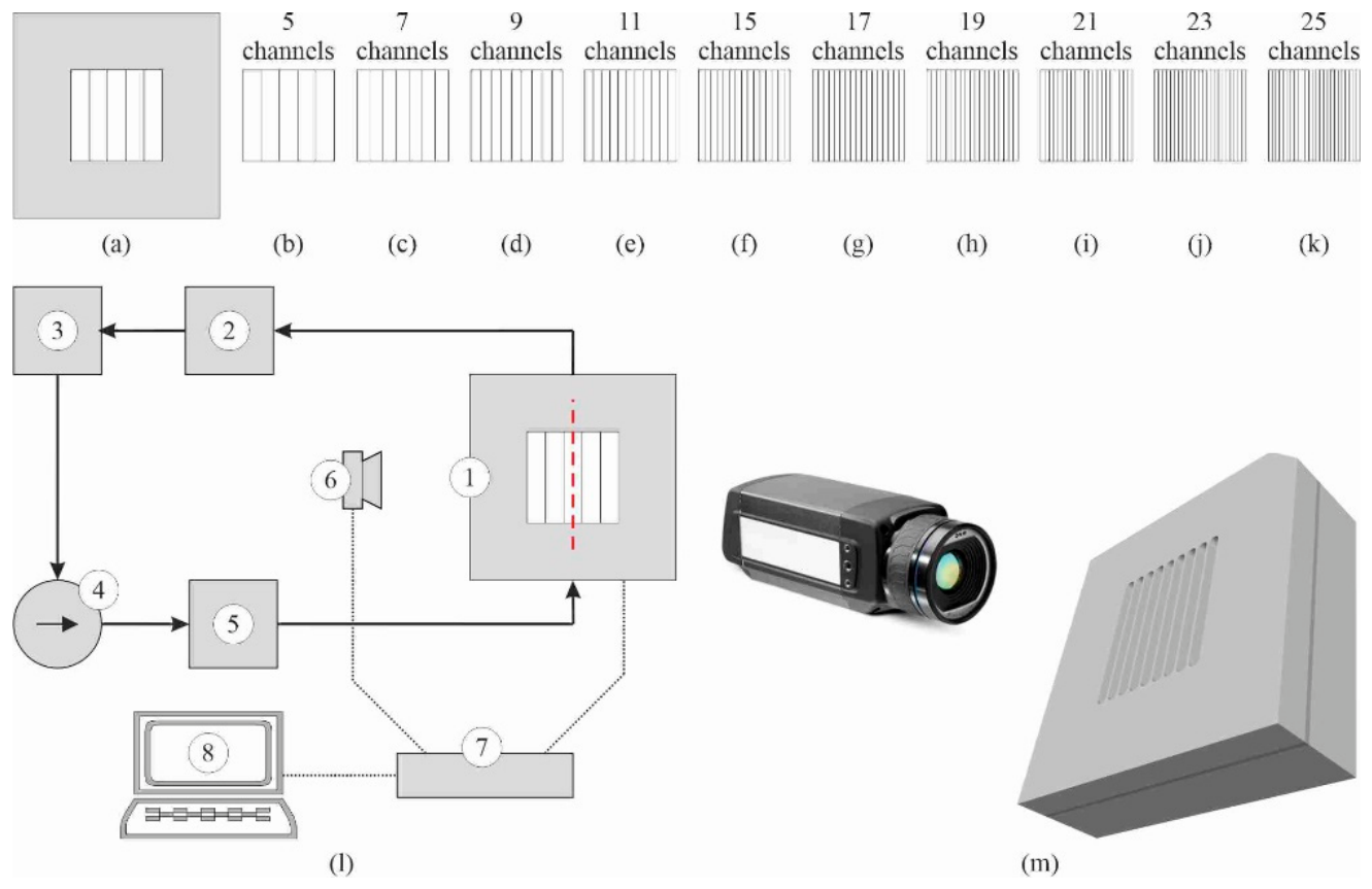
Figure 2.
Traceable processing chain: clean infrared profile → deterministic integrity checks and profile descriptors → supervised anomaly score → retain, review, possible reversible correction, or rejection; retained profiles proceed to downstream thermal reconstruction.
Figure 2.
Traceable processing chain: clean infrared profile → deterministic integrity checks and profile descriptors → supervised anomaly score → retain, review, possible reversible correction, or rejection; retained profiles proceed to downstream thermal reconstruction.
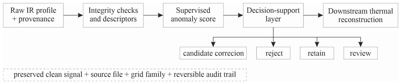
Figure 3.
Representative clean and synthetically modified profiles for the eight primary anomaly morphologies and the global-offset challenge. In the anomaly panels, the dashed blue curve denotes the clean reference profile and the solid orange curve denotes the synthetically modified profile.
Figure 3.
Representative clean and synthetically modified profiles for the eight primary anomaly morphologies and the global-offset challenge. In the anomaly panels, the dashed blue curve denotes the clean reference profile and the solid orange curve denotes the synthetically modified profile.
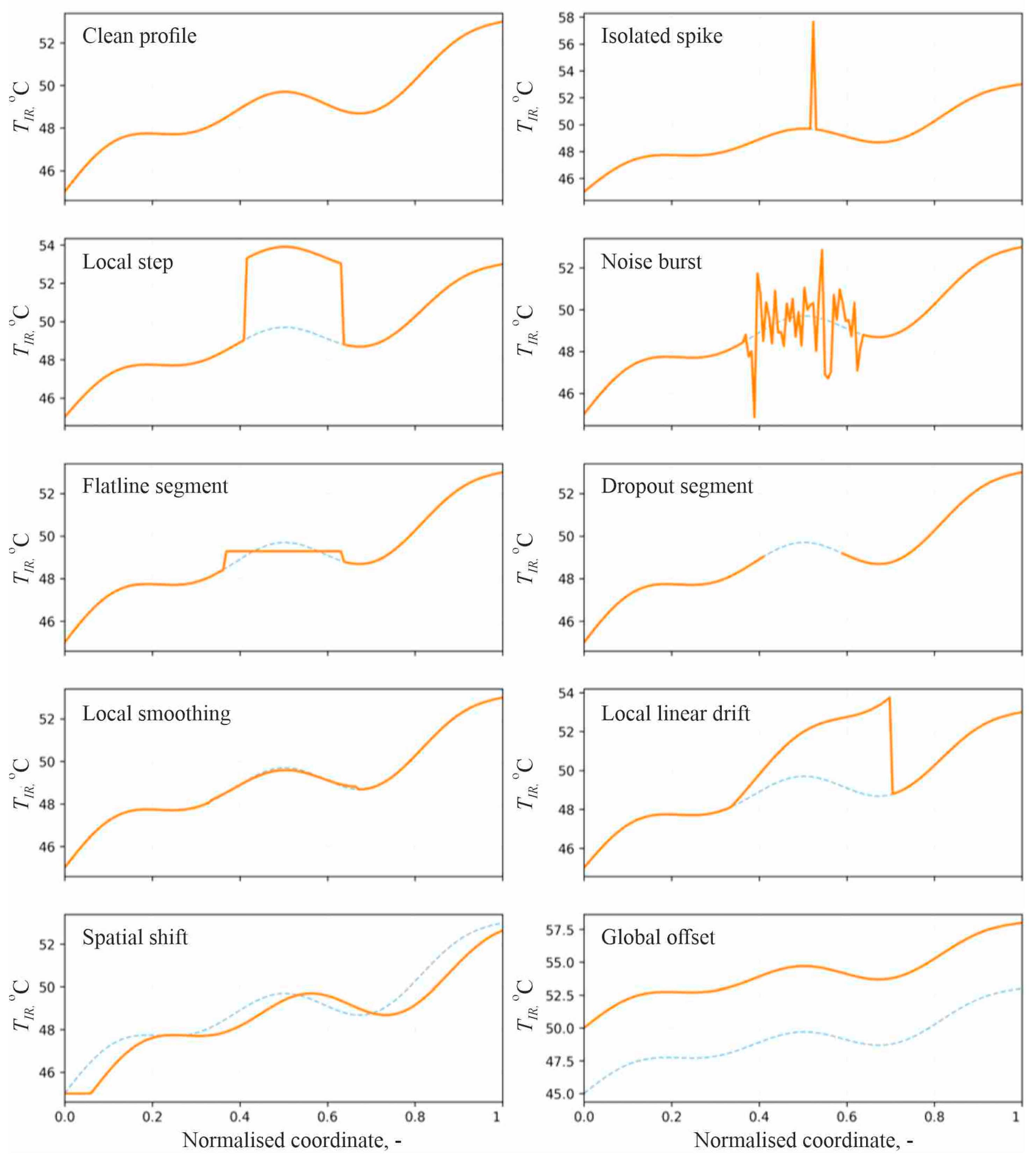
Figure 4.
Leakage-safe development protocol: source-file grouping, train-only fitting, validation-only model and threshold selection, one-time locked test evaluation, and external-grid transfer assessment.
Figure 4.
Leakage-safe development protocol: source-file grouping, train-only fitting, validation-only model and threshold selection, one-time locked test evaluation, and external-grid transfer assessment.
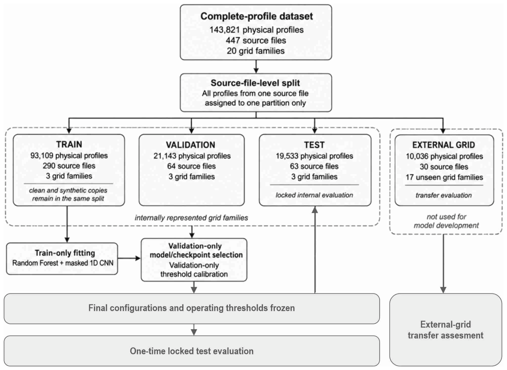
Figure 5.
Receiver operating characteristic and precision-recall curves for the primary synthetic-anomaly benchmark. Panels (a) and (c) show the locked test set, while panels (b) and (d) show the external-grid evaluation. Values in parentheses denote AUROC for ROC panels and AUPRC for precision-recall panels.
Figure 5.
Receiver operating characteristic and precision-recall curves for the primary synthetic-anomaly benchmark. Panels (a) and (c) show the locked test set, while panels (b) and (d) show the external-grid evaluation. Values in parentheses denote AUROC for ROC panels and AUPRC for precision-recall panels.
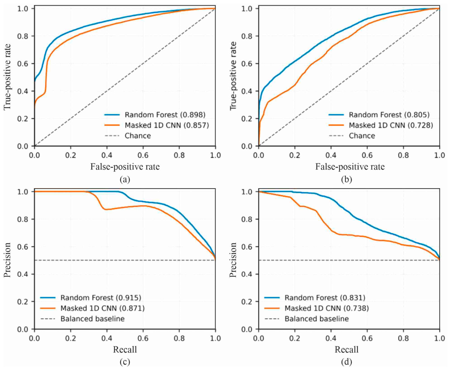
Figure 6.
Weighted sensitivity of the Random Forest and masked 1D CNN for the eight primary anomaly types on (a) the test set and (b) the external-grid set. Low, medium, and high intensities are combined using the number of evaluated physical profiles as weights.
Figure 6.
Weighted sensitivity of the Random Forest and masked 1D CNN for the eight primary anomaly types on (a) the test set and (b) the external-grid set. Low, medium, and high intensities are combined using the number of evaluated physical profiles as weights.
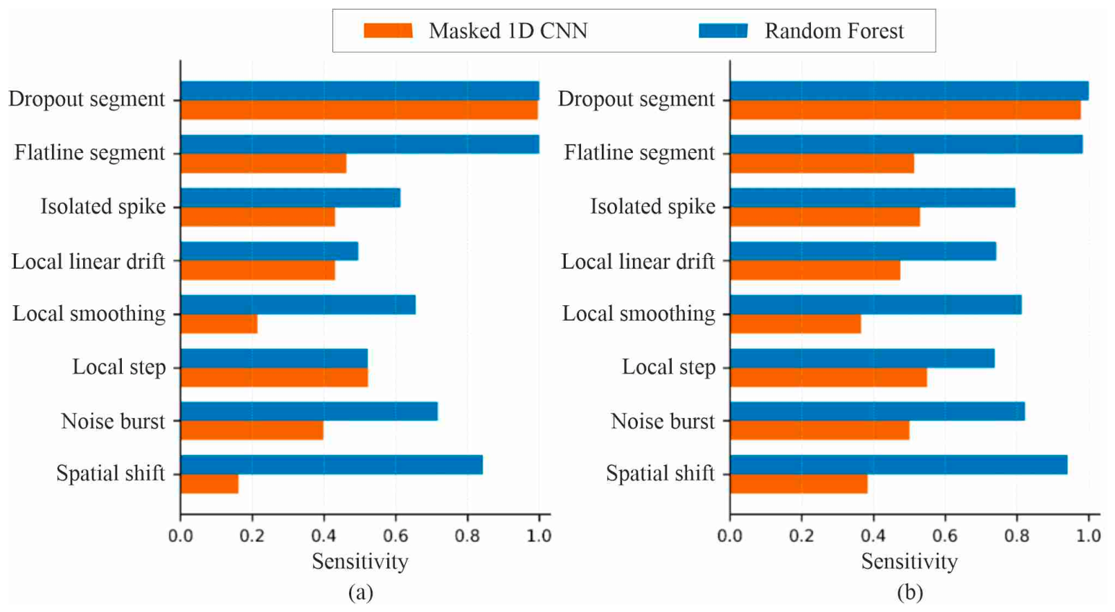
Figure 7.
Transfer characteristics of the masked 1D CNN. Panel (a) compares AUPRC, sensitivity, and FPR for short, intermediate, and long external profile-length classes. Panels (b) and (c) show family-level AUPRC and FPR versus nominal profile length. Marker area is proportional to the number of physical profiles; selected labels identify diagnostic and extreme grid families.
Figure 7.
Transfer characteristics of the masked 1D CNN. Panel (a) compares AUPRC, sensitivity, and FPR for short, intermediate, and long external profile-length classes. Panels (b) and (c) show family-level AUPRC and FPR versus nominal profile length. Marker area is proportional to the number of physical profiles; selected labels identify diagnostic and extreme grid families.
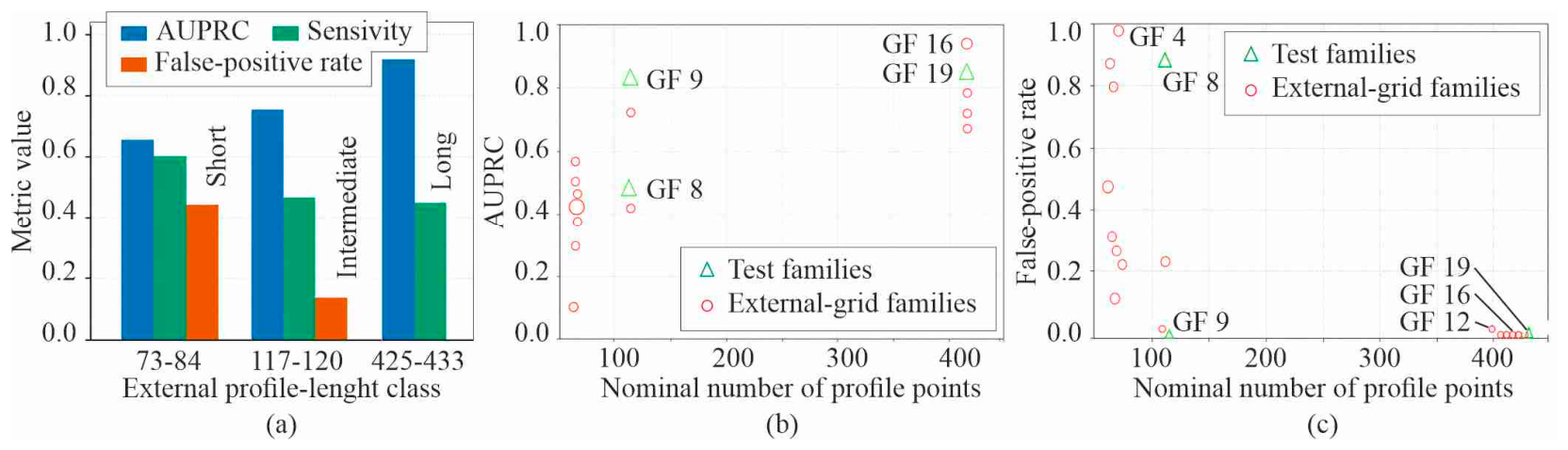
Figure 8.
Additional diagnostic results. Panel (a) shows weighted sensitivity by anomaly intensity on the test and external-grid sets. Panel (b) shows AUROC for the global-temperature-offset challenge relative to the chance level of 0.5.
Figure 8.
Additional diagnostic results. Panel (a) shows weighted sensitivity by anomaly intensity on the test and external-grid sets. Panel (b) shows AUROC for the global-temperature-offset challenge relative to the chance level of 0.5.
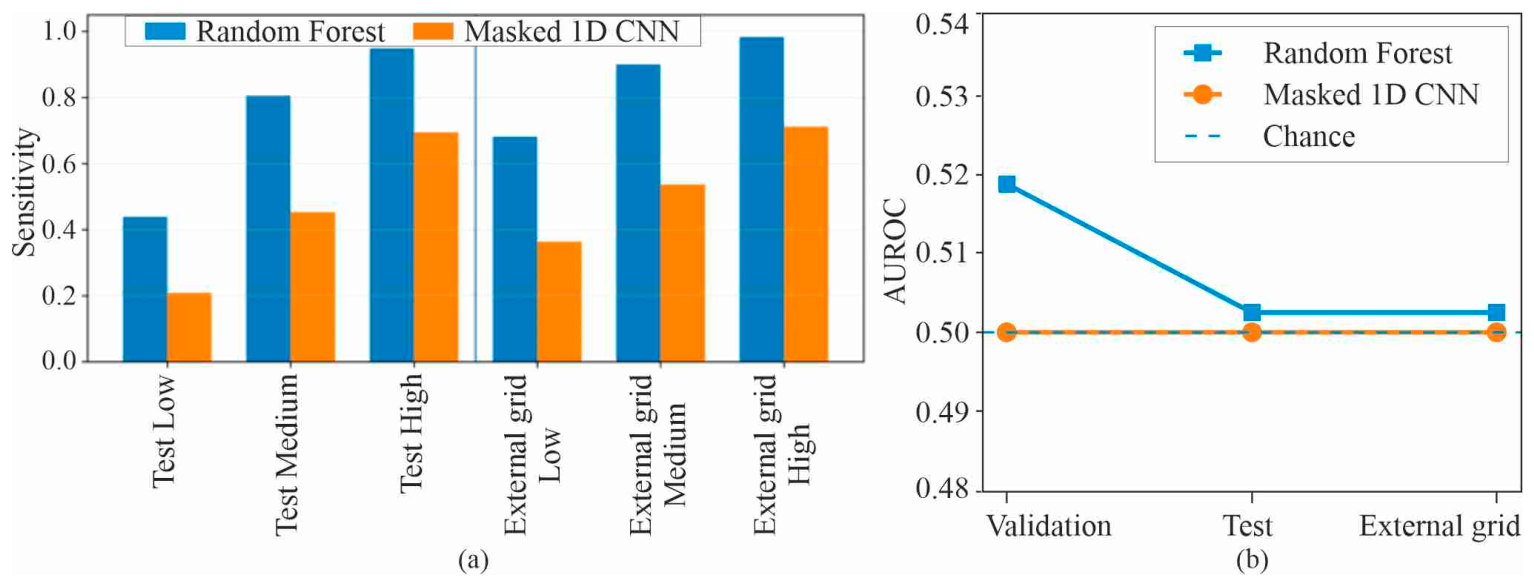

Table 1.
Specifications of the FLIR A655sc infrared camera and thermographic acquisition, radiometric, environmental, and longitudinal-profile extraction settings for the analysed 2021–2022 experimental series.
Table 1.
Specifications of the FLIR A655sc infrared camera and thermographic acquisition, radiometric, environmental, and longitudinal-profile extraction settings for the analysed 2021–2022 experimental series.
| Parameter | Value or configuration represented in the analysed series | Primary verification source |
|---|---|---|
| Infrared camera | FLIR A655sc, A600-Series | Camera identification / manufacturer documentation |
| Detector type and spectral range | Focal-plane array, uncooled microbolometer; spectral range 7.5–14 µm | Manufacturer specification |
| Detector resolution | 640 × 480 px | Manufacturer specification / camera metadata |
| Temperature measurement range and stated accuracy | −40–150 °C; stated accuracy ±2 °C or ±2% of reading | Manufacturer specification |
| Thermal sensitivity / noise-equivalent temperature difference (NETD) | <30 mK at 30 °C | Manufacturer specification |
| Acquisition frequency / frame rate | Full-frame acquisition: 50 Hz | Camera acquisition files / manufacturer specification |
| Lens and field of view | IR lens, focal length 24.6 mm; field of view 25° × 19°; instantaneous field of view 0.68 mrad; f/1.0 |
Lens marking / manufacturer specification |
| Surface coating and emissivity setting | The external, air-facing surface of the heating foil observed by the infrared camera was coated with LCR Hallcrest SPBB (Sprayable Black Backing) black paint of known emissivity, ε = 0.98. The emissivity value was used as a radiometric input parameter. | Experimental protocol / coating identification / previous experimental documentation |
| Radiometric input parameters | Surface emissivity, camera-to-surface distance, ambient-air relative humidity, and ambient-air temperature were specified before infrared acquisition. Their numerical values were assigned for the individual experimental series rather than treated as one common fixed setting for the complete archive. | Published experimental protocol / laboratory records |
| Ambient and optical laboratory conditions | Ambient-air temperature and relative humidity remained stable during individual experiments. The analysed series were acquired in 2021–2022, before installation of the laboratory air-conditioning system. Laboratory shading blinds were closed during experiments to limit changes in external illumination, while the artificial room-lighting conditions remained unchanged across the analysed campaigns. | Experimental protocol / laboratory records |
| Camera-to-surface distance and viewing angle | The camera-to-surface distance varied slightly between experimental series owing to test-module installation and removal; the typical working distance was approximately 0.30–0.40 m. The camera was positioned front-on, with its optical axis approximately normal to the observed foil surface. | Laboratory setup / experimental records |
| Camera self-calibration | The infrared camera performed automatic self-calibration after switch-on before measurements. | Published experimental protocol |
| Thermographic observation arrangement | Temperature distributions were recorded from the external, smooth, air-facing surface of the heated foil. When flow visualisation was performed simultaneously, the high-speed camera observed the test section from the opposite side. | Experimental protocol |
| Central-line extraction rule | A central longitudinal temperature profile was selected from the thermogram along the streamwise direction of the heated foil. | Published experimental protocol / processed-data workflow |
| Profile size in the processed database | 73–434 ordered spatial points, depending on grid family | Frozen profile metadata |
| Thermogram analysis and profile-processing software | Researcher IR 4.0 was used for thermogram analysis and selection of the central longitudinal temperature distribution. | Published experimental protocol |
Table 2.
Principal data blocks linked to each thermographic line profile.
| Data block | Representative variables | Role |
|---|---|---|
| Thermography | Central-line external foil temperature; streamwise coordinate |
Primary diagnostic signal |
| Electrical | Current, voltage, wall/net heat-flux terms |
Thermal consistency checks |
| Boundary conditions | Inlet/outlet temperature; ambient conditions when available |
Reference and plausibility checks |
| Hydraulic | Mass flow; local or reconstructed pressure | Operating context |
| Metadata | Source file; fluid; surface; orientation; geometry |
Provenance and grouped validation |
| Derived quantities | Reconstructed wall temperature; α; Nu; regime/ quality-control (QC) fields |
Downstream thermal analysis |
Table 3.
Source-file-level partition of the complete profile dataset.
| Partition | Physical profiles | Source files | Grid families | Role |
|---|---|---|---|---|
| Train | 93,109 | 290 | 3 | Model fitting |
| Validation | 21,143 | 64 | 3 | Model and threshold selection |
| Test | 19,533 | 63 | 3 | Locked internal evaluation |
| External grid | 10,036 | 30 | 17 | Unseen grid-family transfer |
| Total | 143,821 | 447 | 20 | Frozen complete dataset |
Table 4.
Evidence layers in the traceable quality-assessment framework.
| QC layer | Representative indicators | Possible action |
|---|---|---|
| Data integrity | Missing values; duplicate x; broken profile key | Repair metadata or reject |
| Spatial consistency | First/second differences; flatline; spike; roughness | Flag or review |
| Profile consistency | Global shape; local step; drift; edge behaviour | Flag or review |
| Operating context | Power, flow, neighbouring states, geometry | Support interpretation |
| Optional post-reconstruction consistency | Unstable reconstructed wall temperature, α, or Nu |
Secondary review or candidate exclusion |
| Supervised score | Random Forest or masked 1D CNN anomaly probability | Prioritise review |
Table 5.
Synthetic anomaly taxonomy used for controlled profile-level evaluation.
| Benchmark | Anomaly morphology | Intensity levels | Profile operation |
|---|---|---|---|
| Primary | Isolated spike | Low / medium / high | Signed impulse over 1–3 points |
| Primary | Local step | Low / medium / high | Signed offset over a local segment |
| Primary | Noise burst | Low / medium / high | Local increase in high-frequency noise |
| Primary | Flatline segment | Low / medium / high | Local constant-value segment |
| Primary | Dropout segment | Low / medium / high | Local missing-value segment |
| Primary | Local smoothing | Low / medium / high | Local loss of spatial detail |
| Primary | Local linear drift | Low / medium / high | Local monotonic drift |
| Primary | Spatial shift | Low / medium / high | Displacement of the profile along x |
| Challenge | Global offset | Low / medium / high | Uniform temperature shift |
Table 6.
Final supervised benchmark configurations.
| Model | Input representation | Model size/configuration | Frozen threshold |
|---|---|---|---|
| Random Forest | 64 engineered profile descriptors |
240 trees; depth 22; min leaf 2; max_features 0.50 | 0.68350612 |
| Masked 1D CNN | Five channels, right-padded to 448 points | 1,892,673 parameters; best epoch 12 |
0.99998927 |
Table 7.
Locked primary-benchmark performance of the Random Forest and Masked 1D CNN.
| Evaluation | Model | AUPRC | AUROC | Sensitivity | FPR | Balanced accuracy |
|---|---|---|---|---|---|---|
| Test | Random Forest | 0.915 | 0.898 | 0.731 | 0.082 | 0.824 |
| Test | Masked 1D CNN | 0.871 | 0.857 | 0.452 | 0.063 | 0.695 |
| External grid | Random Forest | 0.831 | 0.805 | 0.855 | 0.487 | 0.684 |
| External grid | Masked 1D CNN | 0.738 | 0.728 | 0.537 | 0.257 | 0.640 |
Table 8.
Weighted sensitivity by anomaly morphology.
| Anomaly morphology | RF test | CNN test | RF external | CNN external |
|---|---|---|---|---|
| Dropout segment | 1.000 | 0.997 | 1.000 | 0.978 |
| Flatline segment | 1.000 | 0.463 | 0.984 | 0.514 |
| Isolated spike | 0.614 | 0.431 | 0.795 | 0.530 |
| Local linear drift | 0.496 | 0.431 | 0.743 | 0.475 |
| Local smoothing | 0.656 | 0.215 | 0.814 | 0.366 |
| Local step | 0.522 | 0.523 | 0.738 | 0.550 |
| Noise burst | 0.717 | 0.398 | 0.822 | 0.501 |
| Spatial shift | 0.844 | 0.162 | 0.943 | 0.384 |
Table 9.
Masked 1D CNN performance by external profile-length class.
| Length class | Families | Profiles | AUPRC | Sensitivity | FPR |
|---|---|---|---|---|---|
| Short profiles, 73-84 points | 8 | 5624 | 0.660 | 0.601 | 0.443 |
| Intermediate profiles, 117-120 points | 2 | 624 | 0.759 | 0.470 | 0.139 |
| Long profiles, 425-433 points | 7 | 3788 | 0.922 | 0.453 | 0.000 |
Disclaimer/Publisher’s Note: The statements, opinions and data contained in all publications are solely those of the individual author(s) and contributor(s) and not of MDPI and/or the editor(s). MDPI and/or the editor(s) disclaim responsibility for any injury to people or property resulting from any ideas, methods, instructions or products referred to in the content. |
© 2026 by the authors. Licensee MDPI, Basel, Switzerland. This article is an open access article distributed under the terms and conditions of the Creative Commons Attribution (CC BY) license (http://creativecommons.org/licenses/by/4.0/).
Copyright: This open access article is published under a Creative Commons CC BY 4.0 license, which permit the free download, distribution, and reuse, provided that the author and preprint are cited in any reuse.