
Submitted:
07 September 2026
Posted:
08 September 2026
You are already at the latest version
Abstract
Background: Public policies are increasingly judged not only by their support for production but by how they shape trade structure, value distribution and resilience to shocks. Romania's sheep sector has expanded since EU accession, yet whether this has translated into higher-value exports or more resilient trade destinations remains unclear. Methods: Using UN Comtrade, FAOSTAT and Eurostat data for 2003–2024, four dimensions — production base, trade orientation, value structure and geographical concentration — were examined via descriptive indicators, Kendall trend tests, permutation Kruskal–Wallis comparisons across five policy periods, and one-sided sign and Wilcoxon tests, with robustness checks in constant prices. Results: The sheep population grew 42.8% (2003–2024), but slaughter and meat production did not follow proportionally, and the Slaughter Rate fell from 83.6% to 51.1%. Live Export Value Share exceeded 50% every year (median 92.2%), and live export value exceeded meat export value in all 22 years (median ratio 11.8). Eight of fourteen indicators differed significantly across policy periods, and geographical concentration was confirmed for meat but not live-animal exports. Conclusions: The sector combines an expanding productive base with a persistently live-animal-centric export structure; policy should complement production support with investment in slaughter and processing capacity, quality classification and market diversification, rather than restricting live exports.
Keywords:
sheep sector
; live animal exports
; value creation
; trade resilience
; agricultural policy
; export concentration
; Romania
1. Introduction
Contemporary agri-food systems operate in an environment characterized by increasing economic interdependencies, price volatility, climate pressures, geopolitical tensions and frequent disruptions to supply chains. In this context, public policies can no longer be evaluated solely on their ability to support agricultural production. Equally important is how they influence the structure of trade, the distribution of value along agri-food chains, producers’ access to markets and the capacity of agricultural sectors to absorb and overcome external shocks. The resilience of a food system involves not only maintaining the availability of products, but also preserving essential economic, social and institutional functions in times of crisis [1,2]. At the same time, the capacity of supply chains to adapt to disruptions depends on the diversity of sources, the flexibility of trade relations and the existence of internal infrastructures capable of supporting production, processing and distribution [3].
International trade helps balance the gap between production and consumption, facilitates access to larger markets and offers producers opportunities for capitalisation. However, expanding trade can also generate new vulnerabilities: integration into international trading systems does not automatically guarantee resilience, especially when exports depend on few products or partner countries. Geographic diversification can improve supply stability, but growing trade dependence can reduce the autonomy of the national food system [4]. Concentrated trade flows and interdependent markets can also favour the rapid transmission of shocks across regions [5,6]. From this perspective, assessing trade performance must go beyond the volumes and values exported to include export structure, market concentration and the national economy’s capacity to retain the value created.
This issue is particularly important in the livestock sectors, where the same productive potential can be exploited through very different business models: animals can be exported live, with slaughter, processing and marketing of the meat taking place in the importing country, or slaughtered and processed domestically for export as chilled or frozen meat, edible organs, hides and other products. These models are not equivalent from the perspective of the agri-food chain’s economic organization. The literature on food chains shows that rural development depends not only on primary production but on the relationships between producers, processors, distributors and final markets [7]. Value-chain analysis identifies the activities through which a product acquires higher economic value and how that value is distributed among participants [8,9].
Participation in international trade can take the form of integration into segments with different levels of processing and complexity. Exporting primary products can provide immediate income and meet well-defined external demand, but the activities contributing most to a product’s final value may take place outside the exporting economy. Studies on global supply-chain fragmentation demonstrate that the gross value of exports is not equivalent to the value added retained in the economy of origin [10,11]. For the livestock sector, this distinction is essential: a high value of live animal exports may indicate commercial success without demonstrating the development of domestic slaughtering, cutting, refrigeration, packaging, certification and marketing activities.
Live animal exports should not, however, be interpreted simplistically as valueless for the national economy: for farmers they offer a quick route to capitalise on production, absorb seasonal domestic demand, and secure liquidity, helping sustain farms and jobs where domestic slaughter capacity or demand for sheepmeat is limited. The public policy question is therefore not whether live exports should be eliminated, but whether the current trade structure balances farmers’ incomes with domestic processing, market diversification and sector resilience.
Sheep farming is of particular economic, social and ecological importance in many European regions: sheep systems make use of pastures unsuited to intensive crop production, help maintain agricultural activity in mountainous and disadvantaged areas, and support the conservation of traditional rural landscapes. At the same time, the sector faces unstable incomes, an ageing farming population, labour shortages, farm fragmentation, high costs and demand fluctuations. Its sustainability therefore depends on harmonising economic objectives with social, environmental and animal-welfare objectives [12,13]. Appropriate technologies, improved management and more efficient marketing channels can support productivity, but results also depend on the institutional framework and public interventions [14].
At EU level, the sheep and goat sector is recognized for its role in maintaining agricultural activity in vulnerable territories, but also for structural difficulties including low producer incomes, limited consumption and dependence on public support [15]. The Common Agricultural Policy influences the sector through direct payments, coupled support, rural development measures, investments, environmental standards and animal welfare conditionality, though its effects are not uniform across Member States or farm types: comparative assessments of European sheep and goat farms highlight important differences in economic, social and environmental performance [16]. The experience of shared pastures in Romania likewise shows that CAP effects are mediated by local institutions, user rights and communities’ ability to access available tools [17].
The Common Agricultural Policy is subject to permanent tension between supporting farm incomes, competitiveness, environmental protection and territorial development, and recent literature shows its instruments need to be more firmly adapted to sustainability objectives and farming-system specificities [18]. Public support can contribute to farm viability [19], but maintaining primary production does not automatically consolidate processing chains, diversify markets, or increase the value retained in rural areas — so evaluating sectoral policies must include effects on the commercial structure, not only on livestock and production.
Romania’s 2007 EU accession profoundly changed the institutional framework of national agriculture. Access to the single market, European standards and CAP instruments created opportunities for modernization, but also highlighted structural differences from the agricultural models prevalent in other Member States [20]. Romanian agriculture has significant productive potential, but commercial performance and competitiveness are shaped by farm fragmentation, processing infrastructure, productivity and operators’ capacity to meet market demands [21] — aspects particularly relevant for the sheep sector, where herd size is not always matched by a proportional capacity for processing and marketing meat.
Quality standardization and carcass grading are mechanisms through which the market can more clearly communicate its requirements to producers. The EUROP classification system’s application in the Romanian cattle sector has highlighted the link between carcass quality, producer payment and a common commercial language [22]; although not directly transferable, this demonstrates the institutional infrastructure needed to move from animal marketing to a standardized, quality-differentiated product. Similarly, rural development policy must manage trade-offs between economic performance, resource use and acceptable environmental impact [23]. Consolidating in-house processing should therefore be conceived not only as economic growth, but as part of responsible rural development.
The issue of value retained in the national economy is also linked to food security. A purely quantitative approach, focused on production or export volume, does not capture how benefits and costs are distributed among producers, processors, consumers and communities: food security also implies institutional responsibility, equity and agri-food systems’ capacity to use resources compatibly with present and future needs [24]. Analyses for Romania and neighboring countries show that agricultural performance coexists with structural vulnerabilities, territorial differences and unequal adaptive capacity [25], and the resource losses associated with meat consumption highlight the need for more efficient use of land, water, energy and raw materials [26]. Value creation must therefore be assessed not only as commercial income, but also in relation to responsible resource use and the sustainable development of rural communities.
Live animal exports also have an ethical and welfare dimension that cannot be fully separated from economic analysis. Sheep transport involves risks from handling, loading density, journey time, water and feed availability, and temperature and resting conditions; the EFSA assessment on small-ruminant transport identifies potential welfare consequences including heat stress, thirst, prolonged hunger, fatigue and restricted movement [27]. Commercial transport of live animals in the EU is regulated by requirements on fitness for transport, means of transport, journey planning and operators’ responsibilities [28]. Journey time significantly influences animal welfare [29], and heat stress is a major risk during long-distance transport in adverse climatic conditions [30].
This dimension does not automatically make live animal exports unjustifiable, but it does require public policy to weigh costs not directly reflected in trade values. A sectoral strategy based predominantly on animal exports must be assessed jointly against farmers’ incomes, trade security, animal welfare, domestic processing capacity and downstream job creation, rather than judged a success on export volume alone.
The need for such an analysis became more evident after the disruptions caused by the COVID-19 pandemic: movement restrictions, labour shortages, temporary closures and changed consumption channels exposed important vulnerabilities in food chains [31]. The Russia–Ukraine conflict subsequently amplified uncertainty around energy, feed, transport and input costs, generating new pressures on trade and food security [32]. These shocks show that trade specialization can be advantageous in stable periods, but becomes a source of vulnerability when a sector depends on few markets, sensitive logistical routes, or a single exported product type.
Despite the economic importance of the Romanian sheep sector, its productive base, live animal exports, meat trade, value retention and geographical concentration of markets have not been analysed together: existing studies typically treat herd evolution, farm performance, CAP support, external trade and animal welfare separately, leaving open whether export expansion has been matched by domestic processing development and whether trade geography provides resilience or dependency.
Starting from this gap, the study assesses the transformation of the Romanian sheep sector over 2003–2024 by relating the evolution of the productive base to the structure of foreign trade, comparing live sheep and mutton exports in volume, value and unit value, and examining the geographical concentration of destination markets, with particular attention to Romania’s EU accession, the successive stages of the Common Agricultural Policy, the COVID-19 pandemic and the recent period of economic and geopolitical instability.
To achieve the stated objective, the study aims to answer four research questions:
- RQ1. To what extent is the Romanian sheep sector oriented towards the export of live animals, compared to the export of sheep meat?
- RQ2. How did the relationship between live sheep exports and mutton exports change during the main periods of agricultural policy and market instability between 2003 and 2024?
- RQ3. To what extent are Romania’s exports of live sheep and mutton geographically concentrated and what implications does this concentration have for trade resilience?
- RQ4. What indications do the volume, value and unit value of exports provide regarding Romania’s capacity to create and retain value within the national sheep chain?
The contribution of the study lies in explicitly differentiating animal exports from value exports: it does not assume meat exports are always superior to live animal exports, nor equate export value with value added retained nationally. The aim is to identify the current structure of commercial valorization and assess whether it balances farmers’ access to external markets, the development of domestic processing and sector resilience — providing an empirical basis for policies aimed at modernizing slaughter and processing units, improving product classification and differentiation, diversifying commercial destinations, and consolidating the position of Romanian producers in agri-food chains.
2. Materials and Methods
2.1. Research Design and Analytical Framework
The research was conceived as a longitudinal quantitative study, with an exploratory and explanatory nature, dedicated to the evolution of the sheep sector in Romania and the way in which it has integrated into international trade systems. The analysis follows the period 2003–2024 and starts from a relevant issue for agricultural policies and rural development: the orientation of Romanian exports towards live animals, compared to the export of sheep meat, which involves additional processing stages before external marketing. The choice of Romania as a case study is justified by the importance of the sheep sector in national animal husbandry, by its role in the economy of some rural regions and by the particularities of the integration of Romanian agriculture into the European single market [17,20,21].
The analytical approach was built around the question of whether the development of foreign trade in sheep was also accompanied by a greater capacity to capitalize on production within the national economy. The export of live animals and the export of meat represent two distinct ways of integration into agri-food chains. The first facilitates the rapid capitalization of production and access of breeders to external demand, especially when the domestic market is limited or seasonal. The second involves the carrying out in the country of origin of activities such as slaughtering, cutting, refrigeration, packaging, certification, storage and marketing. These activities can extend the value chain and distribute income among a larger number of economic operators [7,8,9,10,11].
The distinction between the two trade flows has not been treated as a simple opposition between a favorable and an unfavorable option. Livestock exports can support farmers’ incomes, facilitate market access for farms that lack domestic marketing alternatives, and help maintain livestock activities in rural areas. At the same time, dependence on a single type of exported product or on a limited number of markets can increase the sector’s exposure to sanitary and veterinary restrictions, changes in demand, logistical difficulties, and geopolitical instability [4,5,6]. The research therefore aims to assess the balance between farmers’ immediate access to external markets, the development of domestic processing, and the resilience of the trade structure.
The analytical framework brings together four complementary dimensions. The first dimension is the productive base of the sector and reflects the resources that support economic and commercial activity. The second is the orientation of foreign trade and concerns the relationship between the marketing of live sheep and the marketing of sheepmeat. The third dimension refers to the value structure of exports and the indications it provides on Romania’s positioning in the value chain. The fourth dimension is trade resilience, analyzed through the diversity and geographical concentration of destination markets. These dimensions are examined together because a significant productive base does not automatically lead to the development of processing, and a high value of exports does not guarantee the existence of a diversified and resilient trade structure.
In the study, value creation and retention are approached through the lens of trade structure and domestic processing potential. These concepts are not equivalent to gross value added in the accounting sense. The available data do not include production and processing costs, operator margins, logistics costs or the distribution of income between participants in the value chain. Consequently, the research does not estimate the value added that could have been obtained if the exported animals had been slaughtered and processed in Romania. Export values and unit values are used as indirect indicators of trade orientation and the sector’s positioning in the value chain, in line with the distinction between gross export value and value effectively retained in the economy of origin [10,11].
The policy dimension was integrated by relating sectoral developments to institutional moments and market shocks that marked the period under review. Romania’s accession to the European Union, the successive application of the Common Agricultural Policy instruments, the COVID-19 pandemic and recent economic and geopolitical disruptions provide benchmarks for comparing the evolution of production and trade [17,18,19,20,21,31,32]. This approach does not assume that all observed changes were produced exclusively by the policies or events corresponding to each interval. Prices, exchange rates, external demand, climatic conditions, the sanitary-veterinary situation, processing capacity and operators’ decisions can act simultaneously. Differences between periods are therefore interpreted as temporal and institutional associations, not as definitive evidence of a causal relationship.
In line with the research questions presented in the Introduction, the empirical framework was organized around four hypotheses:
- H1, associated with RQ1, assumes that the Romanian sheep sector is predominantly oriented towards the export of live animals, compared to the export of sheep meat.
- H2, associated with RQ2, assumes that major periods of agricultural policy and market instability are associated with significant changes in production, trade orientation, and export structure.
- H3, corresponding to RQ3, assumes the existence of a relevant geographical concentration of export markets, which may amplify the sector’s vulnerability to external shocks.
- H4, associated with RQ4, assumes that the value of live sheep exports is significantly higher than the value of mutton exports, indicating a trade structure oriented mainly towards the sale of the live animal and less towards the export of the processed product. In the case of H4, the difference between the two values is interpreted as an indication of trade positioning, not as a direct measurement of the value added retained in Romania.
By bringing these dimensions together, the research design allows examining the sheep sector not only in terms of the evolution of livestock, production or total value of trade, but also in terms of how production is capitalized, the markets to which it is oriented and the vulnerabilities associated with this orientation. The proposed framework thus provides a basis for evaluating policies related to supporting farmers, developing slaughtering and processing capacities, standardizing quality, diversifying export destinations and strengthening the resilience of trade chains.
2.2. Data Sources and Study Period
The empirical basis of the research was built by integrating statistical series from four international sources: FAOSTAT, Our World in Data, UN Comtrade and Eurostat. For the robustness analysis of trade values in constant prices, the consumer price index from the United States published by the US Bureau of Labor Statistics was additionally used. The choice of these sources aimed to combine coverage of the production sector with detailed information on trade flows, export destinations and price developments. The main observation unit is Romania–year, and for the analysis of the geographical concentration of exports the base was extended to the Romania–year–trading partner level.
FAOSTAT was the main source for the productive base of the sheep sector. From the Crops and livestock products domain, the series on sheep numbers, number of animals slaughtered for meat and sheep meat production were extracted. The database also contains some auxiliary series on by-products, kept for consistency checks and possible further analyses. The values were imported together with the units of measurement and quality indicators reported by FAOSTAT, so that official, estimated, imputed or other observations from other sources could be identified in the audit phase and in sensitivity analyses [33].
The files downloaded through Our World in Data were used to access easily processed historical series and to cross-check livestock, slaughter and production. Since the metadata of these indicators indicate FAOSTAT as the original source, the Our World in Data observations were not treated as an independent statistical source and were not duplicated in the master database. When the same variable was available in both sources, the FAOSTAT series and its quality indicators took precedence, and the Our World in Data file performed a check for concordance and temporal continuity [34].
The data on foreign trade come from UN Comtrade and include the annual flows reported by Romania for imports and exports, both to the world as a whole and to each trading partner. For each observation, the year, direction of flow, partner, product code, quantity, net weight, primary trade value and flags regarding the reported, estimated or aggregated nature of the record were kept. Trade values are expressed in current US dollars, net weight in kilograms and the quantity of live sheep in heads. World data were used as the benchmark for the annual totals, while information on partners was used to calculate the geographical structure and audit the totals [35]. Tariff codes and aggregation rules are presented separately in section 2.3.
Eurostat provided three sets of complementary indicators. The apro_mt_pann set was used for the number and weight of sheep slaughtered in slaughterhouses, expressed in thousands of heads and thousands of tonnes respectively. The apri_pi_outa set provided nominal and real indices of agricultural production prices for the Live sheep and goats category, with the year 2020 equal to 100. From the economic accounts for agriculture, the aact_eaa01 set, the value of production at basic prices for the same category, expressed in millions of euros, was taken. These series are available in the analysed database for the period 2020–2025 and have a complementary role: they support the interpretation of recent developments and robustness checks, but do not replace the FAOSTAT series on total animals slaughtered, as Eurostat statistics refer to slaughtering reported by slaughterhouses [36].
The main study window is 2003–2024. The interval starts four years before Romania’s accession to the European Union, allowing the construction of a pre-accession reference period, and ends with the most recent year for which the production and trade series used in the main comparisons could be treated as sufficiently complete at the time of download. Although the trade files also include the year 2002, there are no import observations for the eight selected HS6 sheep meat items for that year. The year 2002 was therefore kept in the raw sheets for traceability, but excluded from the symmetric import–export comparisons and from the tests applied to the common window. This decision avoids interpreting the absence of reporting as zero trade value.
Observations are available for 2025 in the UN Comtrade and Eurostat files, but they have been treated as recent and potentially subject to revision or completion. In addition, the FAOSTAT series defining the productive base do not provide the same coverage for 2025 as is necessary to calculate all annual indicators. Consequently, 2025 has not been included in the main estimates, in comparisons between periods or in hypothesis testing. The values for this year can only be presented separately, with descriptive and provisional status, and are not used to formulate inferential conclusions.
For robustness analysis, trade values expressed in current US dollars were converted to constant 2024 dollars using the annual CPI-U series (US city average, all items, not seasonally adjusted; series ID CUUR0000SA0). The use of a dollar deflator is consistent with the currency in which UN Comtrade reports the value of trade and allows for partial separation of nominal growth from the effect of general inflation. This adjustment does not eliminate the influence of the exchange rate nor specific price variations in the sheep sector, limitations discussed in section 2.8 [37].
In the harmonisation process, missing values were kept distinct from zero values and were not filled in by interpolation. Zero was retained only when explicitly stated in the original source and was checked against the available detailed records. Only observations that met the established definitions and units were used for the annual aggregations, and any discrepancies between the World total and the sum of partners were recorded in a data quality register and dealt with by explicit rules. Only one quantitative correction was required in the main series: for the 2024 export of HS code 020430, the World net weight was reported as zero, although the sum of the records by partners was 398,161.072 kg; for the calculation of the aggregate volume, the sum of the partners was used, while the World trade value was retained. The detailed selection, aggregation and harmonisation procedures are presented in section 2.3.
Data Availability Statement: The data were downloaded and verified between 28 May and 4 September 2026. The master database keeps the raw sheets, the harmonised series, the variable dictionary and the quality issues register separately, so that each indicator can be traced back to the observations in the original source. This organisation reduces the risk of mixing up statistical definitions and allows the reproduction of the calculations presented in the following sections.
2.3. Commodity Coverage and Data Harmonization
The product coverage was set so that the trade analysis would capture separately the export of live sheep and the export of the main forms of sheep meat, excluding goat meat. The selection was made at the six-digit level of the Harmonized System (HS), using the codes and descriptions provided by UN Comtrade [35]. The live sheep category is represented by the HS code 010410, and the analytical category sheep meat was constructed by bringing together eight HS6 codes, which differentiate fresh or chilled meat from frozen meat, as well as carcasses from bone-in cuts and boneless meat. The exact structure is presented in Table 1.
HS code 020450, which covers fresh, chilled or frozen goat meat, has been explicitly excluded. This delimitation is necessary because some international series present sheepmeat and goatmeat together, although the two sectors are not equivalent in terms of production base, trade channels or prices. In the master base, the combined sheep and goat meat series from Our World in Data were retained only as auxiliary verification sources and were not used in the construction of the main trade indicators. Similarly, the Eurostat category Live sheep and goats was used only as a complement to the interpretation of prices and production value, not as a substitute for sheep-specific trade or production variables.
The UN Comtrade series for the period under review are reported in several successive versions of the HS nomenclature, identified in the files by the classification codes H2, H3, H4, H5 and H6. Before aggregation, the product codes were converted into a six-digit textual format by filling in the leading zero where it had been removed by the numerical format of the spreadsheet. It was then verified that the nine codes included in the selection retain their relevant economic meaning in the successive versions found in the downloaded database. Therefore, temporal harmonization did not require conversions between different products, but standardization of the code format and the use of the same operational definition throughout the period.
The trade files were filtered for Romania as a reporter, with an annual frequency and a second partner fixed to World. Only the standard Import and Export flows were kept. The Re-import and Re-export categories were not selected in the download used and were not subsequently added to the main flows. Imports and exports were processed separately, so that neither their values nor their quantities were offset. For live sheep, the main quantity was expressed in heads, and the net weight was kept as an additional variable. For meat, the trade volume was measured by net weight, expressed in kilograms, and the primary value, expressed in current US dollars, was used as a value measure [35].
The annual sheep meat total was obtained by summing the values and net weights for the eight HS6 codes included, separately for each year and each direction of flow. At the level of national totals, records where World was the partner were used with priority, as these represent the total reported by Romania to UN Comtrade. The partners’ sum was not added to the World total, which would have produced double counting. Instead, it was calculated separately and used as a tool to check the consistency of the values, quantities and weights reported.
For the geographical analysis, the rule was reversed: all records with a partner equal to World were removed before calculating the indicators by destination. The remaining observations were aggregated on the year–partner–flow combination, and in the case of sheep meat also on all eight HS6 codes. Thus, the same destination appears only once each year for the live sheep category and only once for the sheep meat category. The partners’ shares were calculated from the value of exports, not their weight, to maintain the link with the value dimension of trade. Only the Export flow was used in the analysis of the concentration of destination markets; imports remained available for the balance indicators and descriptive checks.
The duplicate control was performed in two stages. First, identical records were searched for in all imported fields. Then, the combinations of year, flow, partner, second partner and HS code were checked, completed with the corresponding descriptive fields. The final files used for live sheep and mutton did not contain exact duplicates. In situations where multiple rows appeared for the same year and partner because they referred to different HS6 codes, these were not treated as duplicates, but as distinct components of the sheep meat category and were summed only after validation of the product code.
The check of totals compared, for each year, stream and code, the World values with the sums resulting from the partner records. The World total was retained as the primary source when it was available and had a plausible value. Deviations were documented in the data quality register and were not automatically corrected. This rule is important because minor differences between the two levels can arise from rounding, statistical confidentiality, unspecified partners or updates to the database, and systematically replacing the reported total with the sum of partners would introduce an arbitrary rule.
An explicit exception was applied to HS code 020430 for the 2024 export. The World record indicated a quantity equal to zero and the net weight field was blank, although the rows by partner totaled 398,161.072 kg. The World trade value of USD 3,765,343.87 coincided with the sum of the values reported by partners. Consequently, the sum of the weights of the partners was used for the quantity component of the total sheep meat, and the primary value World was retained. The intervention is not a trend-based imputation, but a reconciliation of two levels of the same trade reporting; the year, code, affected field and replacement value were recorded in the audit log.
In the final stage, the harmonised trade series were joined to the production variables by the year key. The units were kept distinct, head for livestock, slaughter and live trade; kilograms for net meat weight; tonnes for meat production; current USD for trade values, and conversions were only made in the indicator formulas that required them. Missing values were left blank, and divisions were not calculated when the denominator was missing or equal to zero. Through this sequence of filtering, standardisation, aggregation and auditing, each indicator in the master database can be traced back to the flow, product code and partner level from which it originates.
2.4. Production, Trade Orientation and Value-Creation Indicators
The indicators were constructed to capture three components of the sheep sector: the use of the productive base, the orientation of trade flows and the value structure of exports. The calculations were performed annually, for Romania, using the harmonized series described in sections 2.2 and 2.3. In the formulas, the index represents the year, and the results of the rate or weight type are expressed as a percentage. The indicators were not calculated when the denominator was absent or equal to zero.The first component of the analysis tracks the relationship between sheep stock, slaughterings, and meat production. The level variables—Sheep Stock (), Sheep Slaughtered (), and Sheep Meat Production ()—were initially analyzed as annual series because their changes provide distinct information about herd size, utilization, and productive output. Two derived indicators were calculated to compare series with different scales.Slaughter Rate () expresses the share of animals slaughtered for meat in the sheep herd in the same year:
where is the number of sheep slaughtered for meat, expressed in heads, and represents the sheep population, also in heads. The indicator is used as a measure of the annual intensity of capitalization through slaughter. It should not be interpreted as an individual probability of slaughter nor as a strict biological rate, since the population is a stock variable, while slaughters constitute an annual flow; animal movements and differences between reporting times can affect the ratio.
Carcass Yield () approximates the average amount of meat produced for each animal reported as slaughtered:
where is the sheep meat production expressed in tonnes, and multiplication by 1000 converts tonnes to kilograms. The result is expressed in kg/head. The indicator combines two FAOSTAT series and should be interpreted as apparent average yield, not as individual weight measured directly in the slaughterhouse. It may reflect the structure by animal category, slaughter weight and the particularities of statistical reporting.
The orientation towards live animal exports was measured by Live Export Intensity (), defined as the ratio between the number of live sheep exported and the national livestock:
where represents Live Export Quantity, expressed in heads. The indicator shows what proportion of the annual productive base is equivalent to the volume of live animal exports. As in the case of the Slaughter Rate, the numerator is a flow and the denominator a stock; therefore, the indicator describes the trade intensity, not the individual route of animals in the herd.
To capture the net trade position, the quantitative balances for live animals and meat were calculated separately. Live Trade Balance () is expressed in heads:
where represents Live Import Quantity. A positive value indicates a quantitative surplus of live sheep exports, and a negative value indicates a volume of imports greater than that of exports.
Meat Trade Balance() is expressed in kilograms:
where and represent Meat Export Net Weight and Meat Import Net Weight, respectively. The two balances have not been summed and have not been directly compared in physical units, since one is expressed in heads and the other in kilograms. Their role is to show Romania’s trade position separately on the two segments. Unit values were calculated as the ratio of the commercial value to the corresponding quantity or weight.
For live sheep, Live Export Unit Value per Head () was defined as follows:
where represents the Live Export Value, expressed in current USD. The result, expressed in USD/head, provides an apparent average value for an exported animal.
Since UN Comtrade also reports the net weight of live animals, the Live Export Unit Value per Kilogram () was additionally calculated:
where represents Live Export Net Weight. The result is expressed in USD/kg. This indicator facilitates a prudent comparison with the unit value of meat, but does not convert the live animal into a meat equivalent: live weight includes components that do not become a marketable product after slaughter, and processing costs and yields are not observed in the basis used.
For sheep meat, the Meat Export Unit Value () was calculated by relating the value of exports to the net weight exported:
where represents Meat Export Value. Similarly, Meat Import Unit Value () was calculated to verify the value profile of imports:
where represents Meat Import Value. Both indicators are expressed in USD/kg. The unit values calculated from UN Comtrade are apparent average values, obtained by dividing the total value by the total quantity, and not observed prices for perfectly homogeneous contracts or products. Their change can simultaneously reflect price variation, HS6 code composition, quality, destination, seasonality and costs included in trade reporting [35].
The value structure of exports was assessed by two complementary weights. Live Value Share () measures the share of live sheep exports in the cumulative value of live sheep and mutton exports:
Meat Value Share () represents the share of meat exports in the same total:
By construction, the two weights satisfy the relationship:
These indicators allow the assessment of the change in the structure of exports without the total size of the sector dominating the comparison. A high value of a indicates that external trade revenues come mainly from the sale of live animals, while an increase in signals a higher participation of sheep meat in the exported value. However, do not directly measure the value added created or retained in Romania. Raw trade data do not separate the cost of the animal, processing, logistics services, intermediaries’ margins and the value of intermediate imports. Consequently, the term value creation is operationalized in this research through proxy indicators of processing and trade structure, in line with the distinction between the gross value of exports and domestic value added [10,11].
For hypothesis testing, the indicators were used in a complementary manner. , and describe the relative orientation towards live or meat exports; , and capture the profile of unit values; and and show the net trade position of each segment. The common interpretation of these measures reduces the risk that a single series (e.g., total export value) is considered sufficient to characterize the performance and value creation capacity of the sheep sector
2.5. Export Market Concentration and Trade Resilience Indicators
The geographical concentration of exports was analysed separately for live sheep and mutton, as the two categories may have different destinations, logistical conditions and degrees of trade dependency. The calculations used annual UN Comtrade records at partner level, after removing aggregated rows where the partner was World. In the case of mutton, the values of the eight HS6 codes were summed for each year–partner combination, before calculating market shares. The indicators were constructed based on the value of exports in current USD, not quantities or weights, to measure the distribution of foreign trade revenues across destinations [35].
The common notation starts from , which represents Export Value to partner i, for trade category x, in year t. The category x takes the value L for live sheep and M for sheep meat alternatively. The total value of exports of the respective category was calculated as follows:
The value share of each partner in the annual total, , was defined by the relationship:
Consequently, ,and the sum of the partners’ shares is equal to 1. Only destinations with a positive export value have been retained in the distribution. The residual categories reported by UN Comtrade, such as Areas, nes (“not elsewhere specified”) and Other Europe, nes, have not been eliminated, as their values are part of the reported trade total. For this reason, partner is used in the sense of reported trade destination and does not always designate an individual country.
Number of Export Partners () represents the number of destinations with positive exports for the category x in the year t:
where is an indicator function, equal to 1 when the condition is met and 0 otherwise. A higher value of indicates a broader geographical base of exports, but does not alone demonstrate the existence of a diversified structure. A high number of partners can coexist with dependence on one or a few dominant destinations; therefore, it was interpreted together with concentration indicators.
To calculate Concentration Ratios, the partners’ shares were ordered in descending order, so that . Concentration Ratio for the Largest Partner () measures the share of the most important destination:
Concentration Ratio for the Three Largest Partners () represents the cumulative weight of the first three destinations:
Similarly, the Concentration Ratio for the Five Largest Partners () was calculated as follows:
Using the function allows the calculation of indicators even if less than three or five destinations are reported in a year. The values of , and are between 0 and 100%. A high value shows that a significant part of the export value is dependent on a small group of markets. Unlike , these indicators do not include the full distribution of shares outside the selected group; however, their advantage is the direct interpretation of the dependence on the first, the first three or the first five partners.
Herfindahl–Hirschman Index () integrates the odds of all partners and gives greater weight to dominant destinations by squaring the odds [38,39]:
In this research, it is expressed on a scale of 0–1. For a given number of partners, the theoretical minimum value is and occurs when exports are equally distributed, and the maximum value is 1 and corresponds to the situation where the entire value is directed towards a single destination. An increase in the index signals a greater concentration, while its decrease indicates a more balanced distribution of the value of exports.
To facilitate comparative interpretation, three categories were established before examining the results: indicates low concentration; indicates moderate concentration; and indicates high concentration. These limits correspond to the thresholds of 1500 and 2500 used in the HHI convention on the 0–10,000 scale [40]. The classification is used in the article as a heuristic reference for describing the concentration of export destinations. It does not represent a legal assessment of competition and does not assume that trading partners are equivalent to the firms analyzed in antitrust policy. To avoid conclusions dependent solely on thresholds, continuous values of are reported together with the assigned category.
Commercial resilience was interpreted by reading the five indicators together. A structure with higher and lower , and was considered relatively more diversified and therefore less exposed to the loss of a single market. Conversely, a dominant share or high value.
2.6. Public-Policy and Market-Shock Periodization
To capture the changes in the Romanian sheep sector in distinct institutional and economic contexts, the 2003–2024 time series has been divided into five sub-periods. The delimitation combines milestones of European integration and the Common Agricultural Policy with two major external shocks, the COVID-19 pandemic and the inflationary and geopolitical instability triggered since 2022. The choice does not aim to arbitrarily fragment the series, but to provide a coherent framework for comparing production, trade orientation, value creation and export resilience under different policy and market conditions.
The first sub-period, 2003–2006, was defined as the Pre-EU Accession Period. This represents the baseline situation prior to accession, marked by the preparation for integration into the single market, the progressive harmonisation of the institutional framework and the adaptation of the agricultural sector to Community requirements. At this stage, Romania did not yet benefit from the full application of the Common Agricultural Policy (CAP) instruments, and the performance of the sheep sector mainly reflects the productive and commercial structure existing before accession [20,21].
The second sub-period, 2007–2013, was called Early EU Membership and First CAP Implementation Period. Romania became a member state of the European Union in 2007 [41], and the period covers the first years of the sheep sector operating within the single market and the first full cycle of application of CAP instruments in Romania. Trade integration, access to direct payments and rural development measures, and adaptation to European standards could simultaneously modify production capacity, the choice between live animal and meat exports, and the geographical distribution of trade flows. The name does not suggest that this was the first historical stage of the CAP at Union level, but rather the first period of its implementation for Romania as a member state.
The third sub-period, 2014–2019, has been defined as the CAP 2014–2020 Pre-Pandemic Period. It corresponds to the years of application of the CAP architecture established for the 2014–2020 cycle, including the rules on direct payments [42], but ends in 2019 to avoid including the exceptional effects of the pandemic in the same analytical window. Therefore, the year 2020 formally belongs to the CAP 2014–2020 programming period, but is separated here on the basis of the market shock. This convention allows for a comparison of a relatively homogeneous phase, prior to the pandemic, with the years in which health and logistical restrictions affected agri-food chains.
The fourth sub-period, 2020–2021, was named the COVID-19 Disruption Period. The interval focuses on the years in which the pandemic disrupted mobility, transport, HoReCa activity, and the functioning of some markets and supply chains, with potential effects on the timing and destination of live animal and meat exports [31,32]. The window includes only two annual observations and, for this reason, the means and differences calculated for this sub-period are interpreted with caution. It is not treated as a stable structural regime, but as an episode of acute disruption.
The fifth sub-period, 2022–2024, was defined as the Inflationary and Geopolitical Shock Period. The delimitation captures the overlap between the consequences of Russia’s invasion of Ukraine, the increase in energy, feed and other input costs, inflationary pressures and uncertainty regarding trade routes and conditions. The European Commission has identified these developments as risks to food security and the resilience of agri-food systems [43]. In the same interval, on 1 January 2023, the CAP 2023–2027 began to be applied through national strategic plans, including the Romanian CAP Strategic Plan [44]. The sub-period label therefore highlights the dominant market shock, without ignoring the change in the policy framework produced within the interval.

Table 2.
Analytical periodization of the study period.
| Years | n | Period label | Analytical reasoning |
| 2003–2006 | 4 | Pre-EU Accession Period | Pre-accession reference; institutional alignment and preparation for European integration. |
| 2007–2013 | 7 | Early EU Membership and First CAP Implementation Period | The first years in the single market and the first complete CAP implementation cycle in Romania. |
| 2014–2019 | 6 | CAP 2014–2020 Pre-Pandemic Period | Application of the CAP 2014–2020 framework before the disruptions associated with the pandemic. |
| 2020–2021 | 2 | COVID-19 Disruption Period | Window of sanitary, logistical and commercial shock; results interpreted with caution. |
| 2022–2024 | 3 | Inflationary and Geopolitical Shock Period | Inflationary and geopolitical pressures, coinciding with the start of the CAP 2023–2027. |
In the sub-period analysis, descriptive statistics were calculated for each indicator for the years available in each window. The sub-periods have different lengths (n = 4, 7, 6, 2, and 3 years, respectively), reflecting the actual duration of institutional stages and shock episodes. This asymmetry is taken into account in the choice and interpretation of the tests presented in Section 2.7; in particular, the estimates for 2020–2021 are not considered equivalent in precision to those obtained for longer intervals.
Periodization has an analytical and institutional function, not one of causal identification. The temporal association between a change in indicators and the onset of a sub-period does not demonstrate that the change was produced by a particular public policy or a single shock. The effects of CAP, trade integration, pandemic, inflation and geopolitical tensions may overlap with technological, climatic, demographic and demand developments that are not isolated by this design. Consequently, comparisons between periods are used to identify differences, ruptures and regularities compatible with changing policy and market contexts, and the results are formulated as temporal associations, not as causal effects.
The same cut-off is applied to all indicators to maintain internal comparability of the analysis. When an indicator is not available for the entire interval, the actual number of observations is reported and the missing data is not filled by interpolation. The sensitivity of the conclusions to the definition of the periods and to the use of commercial values expressed in constant prices is examined separately in the robustness analysis described in Section 2.8.
From a trade resilience perspective, a higher HHI value indicates greater geographical dependence and potential vulnerability to sanitary and veterinary restrictions, regulatory changes, logistical disruptions or geopolitical shocks in key destinations. This interpretation captures a structural dimension of resilience, not the actual observed capacity to recover from each shock.
Annual changes in the indicators were examined both as levels and as a direction of evolution during periods of public policy and market shock defined in section 2.6. The increase in the number of destinations was considered evidence of diversification only if it was accompanied by a reduction in the share of dominant partners or a . Similarly, temporary decreases in concentration were not automatically interpreted as an effect of public policy, since the distribution of exports can be influenced simultaneously by external demand, prices, sanitary-veterinary access, transport costs and the emergence or disappearance of trade agreements.
2.7. Statistical Analysis
The statistical analysis was performed for the annual series 2003–2024. The unit of observation was the calendar year, and the values were grouped, when the analysis required it, into the five sub-periods defined in Section 2.6. The processing followed three complementary levels: describing the distribution and variability of the indicators, comparing the policy and shock sub-periods, and testing the direction or intensity of the relationships formulated by the study hypotheses. No observations were eliminated simply because they had extreme values; each value was checked against the source and kept if it represented a valid record.
2.7.1. Descriptive Statistics and Rates of Change
For each indicator, the number of observations (n), arithmetic mean, median, standard deviation (SD), minimum, maximum and coefficient of variation (CV) were calculated. The mean was used to describe the average level, and the median was reported in parallel because it is less sensitive to exceptional years and asymmetric distributions. For a series x with n observations, the arithmetic mean and sample standard deviation were calculated as follows:
Relative variability was expressed by coefficient of variation, calculated only when the mean was different from zero. In the tables, CV was reported as a percentage:
The change between the first and last year of a period was expressed as a percentage change. For strictly positive indicators, the compound annual growth rate (CAGR) was also calculated:
where x₀ and xₜrepresent the values at the beginning and end of the interval, and T is the number of years between the two observations.
Means, medians, SDs, and CVs were calculated separately for each subperiod, using all available observations. Missing values were not imputed or interpolated; the actual number of observations was retained for each outcome. Given the unequal length of the subperiods, comparisons were based on annual distributions rather than equal weighting of the five intervals.
2.7.2. Distributional Assessment and Selection of Statistical Tests
The normality of the distributions was examined by the Shapiro–Wilk test [45], both for the complete series and within sub-periods where there were at least three observations. For the 2020–2021 interval, which contains only two annual values, a normality test is not informative and was not applied. The result of the Shapiro–Wilk test was interpreted together with the median, dispersion and graphical inspection, not as a single mechanical criterion for choosing the inferential procedure.
Although some complete series did not deviate significantly from normality, the groups were small and unequal (n = 4, 7, 6, 2, and 3), and several commercial indicators showed asymmetry and years with large variations. For this reason, decisions regarding hypotheses were based primarily on nonparametric tests and permutation procedures. Parametric tests were not used as the main basis for accepting or rejecting hypotheses. This choice reduces the dependence of the conclusions on the assumption of normality, but does not eliminate the limitation generated by the small number of observations and the temporal nature of the data.
2.7.3. Period Comparisons and Multiple Testing
The overall differences between the five sub-periods were assessed with the Kruskal–Wallis rank-sum test [46]. Since the group sizes are small and unbalanced, the significance of the H statistic was established by a permutation procedure with 20,000 rearrangements of observations between groups and with a random seed fixed at 20260902, for reproducibility. The null hypothesis was that the distributions of the analyzed indicator do not differ between the five sub-periods. The test was applied to the main indicators of production, commercial orientation, unit value and concentration.
For the family of tests for differences between periods, p-values were corrected using the Benjamini–Hochberg false discovery rate procedure [50]. The conclusion regarding H2 was established based on the adjusted p-values. The magnitude of the overall differences was expressed using the rank-based eta-squared:
where H is the Kruskal–Wallis statistic, k is the number of groups, and N is the total number of valid observations.
Negative values that may arise from this formula in very small samples are interpreted as a null effect and reported as zero. Descriptive differences between sub-periods were presented as means, medians, percentage change, and CAGR. Due to only two observations from the pandemic period, no causal conclusions were made nor firm statements were made regarding individual pairs of periods solely based on a post-hoc comparison.
2.7.4. Hypothesis-Specific Testing
The hypotheses were operationalized before interpreting the results, so that each decision could be traced back to an indicator and an explicit statistical rule. Directional tests were used only when the direction was stated in the hypothesis.
Table 2.
Statistical operationalization of the research hypotheses.
| Hypothesis | Tested component | Operational indicator | Primary test | Null hypothesis |
| H1 | Predominance of live animal exports | Live export value share > 0.50; number of years in which live export value exceeds meat export value. | One-sided exact sign test; median share and annual frequency. | H₀: the probability of annual prevalence is not greater than 0.50. |
| H2 | Differences between periods | Main indicators compared across the five sub-periods. | Permutation Kruskal–Wallis test; Benjamini–Hochberg adjustment; η²H. | H₀: the distributions do not differ between sub-periods. |
| H3 | Geographical concentration of exports | HHI compared to the 0.25 threshold, separately for live sheep and sheep meat; CR1, CR3, CR5 and NEP. | One-sided one-sample Wilcoxon signed-rank test; concentration classes and shares. | H₀: the median HHI does not exceed 0.25. |
| H4 | The difference between the value of live exports and the value of meat exports | Annual live export value versus annual sheep meat export value, paired by year. | One-sided paired Wilcoxon signed-rank test; rank-biserial correlation. | H₀: live export value is not greater than meat export value. |
For H1, dominance was defined as an annual Live Export Value Share greater than 0.50. The frequency of years meeting this condition was assessed by a one-sided exact sign test, with a reference probability of 0.50. The median of the share was reported as a measure of the intensity of dominance. H1 and H4 are conceptually close, but not identical: H1 tests for the persistence of the sector’s orientation towards live animals across years, while H4 tests the magnitude and direction of pairwise annual differences between the two export values.
For H3, the HHI was compared with the threshold of 0.25, corresponding to a highly concentrated market according to the interpretation rule set out in Section 2.5 [40]. The one-sided one-sample Wilcoxon signed-rank test [47] was applied separately to the HHI series for live sheep exports and sheep meat exports. CR1, CR3, CR5, NEP and regional distribution were used as complementary structural evidence; thus, a conclusion on concentration was not based on a single indicator.
For H4, the values of live animal and sheep meat exports in the same year were treated as paired observations. A one-sided paired Wilcoxon signed-rank test [47] was applied, with the alternative Live Export Value > Sheep Meat Export Value. The effect size was expressed by rank-biserial correlation:
where W⁺ is the sum of the ranks of the positive differences, and n is the number of non-zero pairs.
R-valuesᵣᵦclose to 1 indicate a consistent dominance of the value of live animal exports, values close to −1 indicate dominance of the value of meat exports, and values close to zero indicate differences without a consistent direction.
2.7.5. Trend and Structural-Change Analysis
Monotonic trends over the entire period 2003–2024 were assessed by Kendall’s tau-b correlation between Year and Indicator [48]. The test was two-sided, as the analysis tracked both upward and downward trends. The τ coefficient served simultaneously as an association statistic and as a measure of the strength and direction of the trend.
where C and D are the numbers of concordant and discordant pairs, and Tₓ and Tᵧrepresents the adjustments for equalities.
To examine whether EU accession coincided with a change in level or slope, an interrupted segmented regression model with a breakpoint in 2007 was additionally estimated:
The variable Time represents the annual trend since 2003; Post2007 has the value 0 before 2007 and 1 since 2007; TimeAfter2007 is 0 before accession and increases annually since 2007. The coefficient β₂ expresses the immediate change in level, and β₃ the change in slope after accession. For strictly positive indicators, the natural logarithm transformation was used. Standard errors were calculated with the Newey–West heteroskedasticity and autocorrelation consistent covariance estimator, with lag 1 [49]. Due to the small number of years before accession and the absence of a control group, the segmented regression was treated as an associative analysis and not as the identification of a causal effect.
2.7.8. Significance Level, Reporting and Software
The statistical significance level was set at α = 0.05. P values were reported two-sided, except for directional tests specified for H1, H3, and H4. Results with p < 0.05 were considered statistically significant, but interpretation also took into account the effect size, the stability of the result in the robustness analysis, and the economic relevance. Very small p values were reported as p < 0.001, and other values to three decimal places, without equating the lack of statistical significance with the absence of an effect.
The analysis was performed in Python 3.12.13, using pandas 2.2.3 for data organization, NumPy 2.3.5 for numerical operations, and SciPy 1.17.0 for statistical tests [51]. Permutation procedures and segmented regression estimation with Newey–West HAC(1) were reproducibly implemented in the analysis scripts. All calculations were performed both on the basis on nominal commercial values and, where relevant, on the basis of values expressed in constant 2024 USD, according to the robustness analysis presented in Section 2.8.
2.8. Robustness Analysis and Methodological Limitations
The robustness analysis aimed to determine whether the main conclusions depended on the monetary expression of trade flows, the presence of exceptional years, the inclusion of provisional data for 2025, or the correction of a quantitative mismatch. The checks were applied to the same indicators and statistical decision rules presented in Section 2.7. Robustness was defined as the maintenance of the direction of the result, the conclusion on statistical significance and, where relevant, the hypothesis framing after controlled changes to a single methodological choice. Full methodological details and the complete robustness and sensitivity results (Table S1–S3, Figure S1) are provided in the Supplementary Materials.
2.8.1. Methodological Limitations
Several methodological limitations apply throughout the analysis and are discussed together with their implications in Section 4.6: export unit values are aggregate ratios rather than observed prices for a homogeneous product; the database does not include farm-, slaughterhouse- or processor-level cost and margin data needed to estimate value added; comparable data on slaughterhouse capacity, utilisation and territorial distribution are not available; the underlying data sources differ in coverage, definitions and revision practice; and the annual, unequal-length sub-periods may mask seasonal patterns and reduce the power to detect short-term disruptions.
3. Results
3.1. Evolution of the Romanian Sheep Production Base
Between 2003 and 2024, the production base of the Romanian sheep sector followed a divergent evolution. The sheep population expanded almost continuously, but this growth was not accompanied by a comparable increase in the number of animals slaughtered or in meat production. Figure 1 highlights the gradual separation between the size of the herd and the productive outcomes associated with slaughter.
The sheep population increased from 7.312 million heads in 2003 to 10.443 million in 2024, which represents an increase of 42.83%, calculated according to Equation (23). The value in 2003 was the minimum of the entire series, and that in 2024, the maximum. The trend, assessed by Kendall’s tau-b according to Equation (27), was strongly upward and statistically significant (τ = 0.861; p < 0.001). The average population, calculated according to Equation (20), rose steadily across all five periods, from 7.449 million heads before accession to 10.330 million in 2022–2024 (Table 3). The differences between the five sub-periods, tested by the Kruskal–Wallis permutation procedure described in Section 2.7, were significant (H = 18.316; adjusted p < 0.001), and the rank-based effect size, calculated according to Equation (25), was high (η²H = 0.842).
In contrast, the number of animals slaughtered did not show a significant monotonic trend, based on Kendall’s tau-b calculated according to Equation (27) (τ = 0.108; p = 0.503). The series started from 6.115 million heads in 2003 and reached 5.334 million in 2024, resulting in a 12.76% decrease between the ends of the interval, according to Equation (23). The maximum level, 7.737 million heads, was recorded in 2016, after which slaughters decreased noticeably. The average increased from 5.392 million heads in the period 2003–2006 to 6.028 million in 2007–2013 and 6.256 million in 2014–2019, but dropped to 5.305 million during the pandemic years. In the period 2022–2024, the average partially recovered to 5.590 million head, without returning to the level of the period 2014–2019. The overall comparison of the five sub-periods was not significant after correction for multiple testing (H = 6.279; adjusted p = 0.245; η²H = 0.134); the effect size η²H was determined according to Equation (25).
Sheep meat production was more volatile than livestock. It decreased from 62,100 tons in 2003 to 51,690 tons in 2024, or 16.76%, based on the percentage change defined by Equation (23). The minimum of the series, 41,993 tons, was recorded in 2006, and the maximum, 77,375 tons, in 2016. Over the entire interval, there was no significant monotonic trend, assessed according to Equation (27) (τ = 0.091; p = 0.577). The overall differences between the five sub-periods were also not significant after correction for multiple testing (H = 3.392; adjusted p = 0.576; η²H = −0.036), η²H being calculated according to Equation (25). The average production reached its highest level in 2014–2019, at approximately 64.44 thousand tons, but decreased to 52.07 thousand tons in 2020–2021 and remained at only 54.85 thousand tons in the period 2022–2024.
The divergence between livestock numbers and their productive use is summarized by the Slaughter Rate, calculated according to Equation (1). The ratio of slaughtered animals to total livestock decreased from 83.63% in 2003 to 51.08% in 2024, a decrease of 32.55 percentage points. The downward trend, assessed according to Equation (27), was significant (τ = −0.420; p = 0.006). The average of the indicator progressively decreased from 72.47% in 2003–2006 and 70.45% in 2007–2013 to 64.09% in 2014–2019 and 52.11% during the pandemic period. The recovery to 54.13% in 2022–2024 was modest compared to previous levels. The global test indicated differences between the subperiodic distributions before correction, but these did not remain significant after the Benjamini–Hochberg adjustment described in Section 2.7 (H = 8.464; adjusted p = 0.084; η²H = 0.263); the effect size was calculated according to Equation (25).
Carcass Yield, calculated according to Equation (2), remained relatively stable at the aggregate level. The indicator varied between 8.15 kg/head in 2006 and 12.83 kg/head in 2004, and the values at the beginning and end of the period were close: 10.16 kg/head in 2003 and 9.69 kg/head in 2024. No significant monotonic trend was identified based on Equation (27) (τ = −0.022; p = 0.911). The overall differences between the five sub-periods were also not significant (H = 1.276; adjusted p = 0.886; η²H = −0.160), the effect size being determined according to Equation (25). The sub-periodic averages were within a narrow range, between 9.81 and 10.25 kg/head, which shows that the reduction in meat production in relation to the expansion of the herd was not mainly determined by a sustained deterioration in the average yield per slaughtered animal.
Overall, the results depict a numerically expanding livestock base, but with a decreasing conversion of livestock into slaughter and meat production. At the end of the period, Romania had more sheep than at the beginning, but slaughtered fewer animals and produced less meat. This discrepancy provides the quantitative context for the analysis of the orientation towards live animal exports presented in Section 3.2.
Table 4.
Trend and between-period tests for the Romanian sheep production-base indicators, 2003–2024.
Table 4.
Trend and between-period tests for the Romanian sheep production-base indicators, 2003–2024.
| Indicator | τ | Trend p | H | Adjusted p | η²H | Statistical conclusion |
| Sheep stock | 0.861 | <0.001 | 18,316 | <0.001 | 0.842 | Increasing trend; significant period differences |
| Sheep slaughtered | 0.108 | 0.503 | 6,279 | 0.245 | 0.134 | No significant trend or period differences |
| Sheep meat production | 0.091 | 0.577 | 3,392 | 0.576 | −0.036 | No significant trend or period differences |
| Slaughter Rate | −0.420 | 0.006 | 8,464 | 0.084 | 0.263 | Decreasing trend; period differences not significant after adjustment |
| Carcass Yield | −0.022 | 0.911 | 1,276 | 0.886 | −0.160 | No significant trend or period differences |
Notes: N = 22 for all indicators. Trend p-values correspond to Kendall’s τ calculated according to Equation (27). Adjusted p-values for permutation Kruskal–Wallis tests were obtained using the Benjamini–Hochberg procedure described in Section 2.7 across the complete family of 14 between-period comparisons. η²H is the rank-based effect-size estimate calculated according to Equation (25). Negative η²H estimates may occur when H < k − 1 and are interpreted as no detectable effect. Statistical significance was assessed at p < 0.05.
3.2. Live Sheep versus Sheep Meat Export Orientation
The analysis of trade flows confirms that the expansion of the production base presented in Section 3.1 has been accompanied by a persistent external orientation towards the trade of live animals. However, this orientation has not remained unchanged in all its dimensions. Mutton exports have increased substantially compared to the level at the beginning of the period, while the intensity of live sheep exports has fluctuated and decreased in recent years. Figure 2 separates the two planes of comparison: the volume and intensity of live animal exports, and the value structure of live sheep and mutton exports, respectively.
The number of live sheep exported ranged from 1.519 million heads in 2006 to 2.995 million in 2019. Although the 2024 value of 1.771 million heads was 4.98% lower than that of 2003, the series presented a significant monotonic upward trend over the 22 years (τ = 0.515; p < 0.001), evaluated according to Equation (27). This seemingly contradictory combination is explained by the high levels reached in the middle and end of the range, followed by the decline in 2024. Annual average exports rose from 1.739 million head before accession to a peak of 2.576 million during the pandemic years, before easing to 2.131 million in 2022–2024 (Table 5).
Live Export Intensity, calculated according to Equation (3), shows that live animal exports represented annually the equivalent of 17.0–28.9% of the national livestock. The average of the indicator ranged from 23.37% before accession to a high of 25.31% during the pandemic years, before dropping to 20.65% in 2022–2024; the 2024 value of 16.96% was the lowest in the entire series. However, the monotonic trend for the full period was not significant (τ = 0.195; p = 0.217). Therefore, the increase in the livestock and value of live animal exports cannot be interpreted as a linear and continuous intensification of the share of the livestock oriented towards exports.
Sheep meat exports increased from 458.9 tonnes in 2003 to 4,433.3 tonnes in 2024, corresponding to an increase of 866.10%, calculated according to Equation (23). The trend in the exported volume was positive and significant (τ = 0.506; p < 0.001). The highest average, 7,079.9 tonnes per year, was recorded during the period 2014–2019, when exports reached a maximum of 9,470.7 tonnes in 2019. Subsequently, the average decreased to 3,504.1 tonnes during the pandemic years and to 2,977.7 tonnes in the period 2022–2024. The result shows that Romania has expanded its capacity to export meat compared to the beginning of the period, but this evolution has not been stable and has not replaced the commercial dominance of live animals.
The value structure provides the most direct verification of the orientation formulated by H1. Live Export Value Share, calculated according to Equation (10), exceeded the 50% threshold in each of the 22 years analyzed. The annual values ranged from 81.80% in 2015 to 97.67% in 2003, and the median for the entire period was 92.20%. In addition, Meat Export Value Share, defined by Equation (11), did not exceed 18.20% in any year. One-sided exact sign test confirmed that the frequency of years in which Live Export Value Share was higher than 0.50 significantly exceeded the reference probability of 0.50 (22 out of 22 years; p < 0.001). Consequently, H1 is supported.
The dominance of live animals was persistent, but its value intensity varied between sub-periods. The average share of live exports decreased from 94.33% before accession to 85.45% in 2014–2019, when meat exports had the largest relative contribution, before recovering to 93.61% and 92.68% in the two most recent periods. The overall differences between the five sub-periods were significant after the Benjamini–Hochberg adjustment described in Section 2.7 (permutation Kruskal–Wallis H = 9.689; adjusted p = 0.045; η²H = 0.335), the effect size being calculated according to Equation (25). However, for the entire series no significant monotonic trend in the weight was identified (τ = −0.203; p = 0.197).
Table 6.
Trend and hypothesis tests for export-orientation indicators, 2003–2024.
| Indicator / test | N | Statistical | p | Adjusted p | η²H | Statistical conclusion |
| Live sheep export quantity – Kendall trend | 22 | τ = 0.515 | <0.001 | - | - | Significant increasing trend |
| Sheep meat export volume – Kendall trend | 22 | τ = 0.506 | <0.001 | - | - | Significant increasing trend |
| Live Export Intensity – Kendall trend | 22 | τ = 0.195 | 0.217 | - | - | No significant monotonic trend |
| Live Export Value Share – Kendall trend | 22 | τ = −0.203 | 0.197 | - | - | No significant monotonic trend |
| Live Export Value Share - period comparison | 22 | H = 9.689 | 0.025 | 0.045 | 0.335 | Significant period differences |
| H1 – one-sided exact sign test | 22 | 22/22 > 0.50 | <0.001 | - | - | H1 supported |
Notes: Kendall’s τ was calculated according to Equation (27). The adjusted p-value for the period comparison belongs to the complete family of 14 permutation Kruskal–Wallis tests and was obtained using the Benjamini–Hochberg procedure described in Section 2.7. η²H was calculated according to Equation (25). H1 used the annual predominance threshold Live Export Value Share > 0.50. Statistical significance was assessed at p < 0.05.
Taken together, the results indicate an incomplete transformation of the trade profile. The increase in meat exports, especially in the period 2014–2019, shows that the processed segment may gain greater relevance. However, the fact that over four-fifths of the combined value of exports came from live sheep each year demonstrates the persistence of a live-animal-centric trade model. This finding describes the way in which the sector accesses external markets; it does not directly measure the value added retained in Romania. The differences between the values and unit values of the two flows are analyzed separately in Section 3.3.
3.3. Export Unit Values and Value-Creation Proxies
The analysis of trade values and unit values completes the picture of export orientation presented in Section 3.2. However, the two dimensions must be separated. The total value of exports shows the monetary magnitude of each flow, while export unit value relates the declared value to the quantity exported. Figure 3 shows the evolution of the two categories of indicators, and the delimitation of sub-periods allows the observation of changes associated with different institutional and market contexts.
The nominal value of live sheep exports increased from USD 81.93 million in 2003 to USD 282.72 million in 2024, an increase of 245.09%, calculated according to Equation (23). The trend was strongly upward and statistically significant (Kendall’s τ = 0.861; p < 0.001), based on Equation (27). The annual average rose from USD 90.87 million before accession to a peak of USD 295.41 million in the pandemic years, then held at USD 289.86 million in 2022–2024 (Table 7). The differences between subperiods were significant and had a very large effect size (H = 18.449; adjusted p < 0.001; η²H = 0.850).
Sheep meat exports started from a much lower base, but had a larger relative increase: from 1.95 million USD in 2003 to 39.61 million USD in 2024, respectively +1,927.38%, according to Equation (23). The trend was positive and significant (τ = 0.550; p < 0.001). Average meat exports peaked at 34.94 million USD in 2014–2019 before declining to 19.78 and 23.19 million USD in the two most recent periods. The comparison between periods indicated significant differences, with a large effect (H = 15.365; adjusted p < 0.001; η²H = 0.669). The growth of the meat segment is therefore visible, but it has not eliminated the gap with live animal exports.
The gap between the two flows is summarized by the Live-to-Meat Export Value Ratio. The ratio decreased from 41.94 in 2003 to 7.14 in 2024, i.e., by 82.98%, and the median for the entire period was 11.81. The ratio’s lowest average, 6.25, occurred in 2014–2019, when meat exports acquired the greatest relative importance, before returning to 15.31 and 15.63 in the two most recent periods. The reduction compared to the initial year indicates some diversification towards meat, but in each year the value of live sheep exports remained higher than the value of meat exports.
Live Export Unit Value per Head, calculated according to Equation (6), increased from 43.96 USD/head in 2003 to 159.65 USD/head in 2024 (+263.19%). The trend was strongly upward (τ = 0.792; p < 0.001), and the differences between periods were significant, with a large effect size (H = 16.671; adjusted p < 0.001; η²H = 0.745). The average of the indicator increased progressively from 52.90 USD/head before accession to 137.85 USD/head in 2022–2024. This result reflects the increase in the declared value per exported animal, without allowing the separation of the price effect from changes in the weight, breed, quality or destination of the animals.
Sheep Meat Export Unit Value, calculated according to Equation (8), increased from 4.26 USD/kg in 2003 to 8.93 USD/kg in 2024 (+109.85%). Unlike the indicator for live animals, the series did not show a significant monotonic trend for the entire period (τ = 0.126; p = 0.434), as the increase in the first years after accession was followed by a decrease in the period 2014–2019 and a recovery after 2020. However, the overall differences between the sub-periods were significant (H = 13.426; adjusted p = 0.002; η²H = 0.554), and the highest average, 7.39 USD/kg, was observed in 2022–2024.
Table 8.
Trend, between-period and paired-value tests for export-value indicators, 2003–2024.
| Indicator / test | N | Statistical | p | Adjusted p | Effect size | Statistical conclusion |
| Live export value – Kendall trend | 22 | τ = 0.861 | <0.001 | - | τ = 0.861 | Significant increasing trend |
| Meat export value – Kendall trend | 22 | τ = 0.550 | <0.001 | - | τ = 0.550 | Significant increasing trend |
| Live Export Unit Value – Kendall trend | 22 | τ = 0.792 | <0.001 | - | τ = 0.792 | Significant increasing trend |
| Meat Export Unit Value – Kendall trend | 22 | τ = 0.126 | 0.434 | - | τ = 0.126 | No significant monotonic trend |
| Live export value - period comparison | 22 | H = 18,449 | <0.001 | <0.001 | η²H = 0.850 | Significant period differences |
| Meat export value - period comparison | 22 | H = 15.365 | <0.001 | <0.001 | η²H = 0.669 | Significant period differences |
| Live Export Unit Value - period comparison | 22 | H = 16.671 | <0.001 | <0.001 | η²H = 0.745 | Significant period differences |
| Meat Export Unit Value - period comparison | 22 | H = 13.426 | 0.001 | 0.002 | η²H = 0.554 | Significant period differences |
| H4 – paired live versus meat export value | 22 | W = 253.0 | <0.001 | - | r_rb = 1,000 | H4 supported |
Notes: Kendall’s τ was calculated according to Equation (27). Adjusted p-values for permutation Kruskal–Wallis tests were obtained using the Benjamini–Hochberg procedure described in Section 2.7 across the complete family of 14 between-period comparisons. η²H and rank-biserial correlation (r_rb) were calculated according to Equations (25) and (26), respectively. H4 used a one-sided paired Wilcoxon signed-rank test with the alternative Live Export Value > Sheep Meat Export Value. Statistical significance was assessed at p < 0.05.
The pairwise comparison of annual values provides a direct test of H4. In all 22 years, Live Export Value was higher than Sheep Meat Export Value. One-sided paired Wilcoxon signed-rank test confirmed the difference (W = 253.0; p < 0.001), and the rank-biserial correlation calculated according to Equation (26) was r_rb = 1.000, indicating the same direction of the difference for all annual pairs. Therefore, H4 is supported. This result is distinct from H1: H1 verified the persistence of the share of live animals above 50% in the combined value, while H4 directly compares the magnitude of the values of the two flows in paired annual observations.
The results describe an increase in the trade value associated with both forms of export, but also the persistence of a net value advantage of the flow of live animals. However, export values and export unit values are only proxies for the form of value creation and trade. They do not measure the value added retained in Romania and do not include costs, margins, processing yields or revenues from by-products. Consequently, the dominance of the value of live exports does not demonstrate that this option maximizes domestic economic value, nor that full transformation into meat would automatically produce higher net gains. It shows that, in the observed trade structure, most of the exported value left the sector in the form of live animals. The geographical dimension and resilience of this structure are analyzed in Section 3.4.
3.4. Geographical Concentration and Trade Resilience
The trade resilience of the sheep sector depends not only on the volume of exports but also on their distribution across markets. A larger number of partners can expand trade options, but does not guarantee diversification when a dominant part of the value remains concentrated in a few destinations. In this section, the Number of Export Partners (NEP), CR1, CR3, CR5 and HHI have been used together to assess the geographical exposure of live sheep and sheepmeat exports. Figure 4 shows the evolution of the HHI and the number of partners.
For live sheep exports, the NEP calculated according to Equation (15) increased from 16 partners in 2003 to 23 in 2024, and the trend was positive and significant (Kendall’s τ = 0.593; p < 0.001), based on Equation (27). The maximum of 32 partners was reached in 2019. However, the expansion of the trade network was not accompanied by a monotonic reduction in concentration. The HHI, calculated according to Equation (19), ranged between 0.130 in 2019 and 0.357 in 2013, with no significant trend over the entire period (τ = 0.056; p = 0.738). The 2024 value of 0.199 indicates a moderate level of concentration following the thresholds set out in Section 2.5.
Concentration ratio indicators confirm that the diversification of live exports remained incomplete. In 2024, the main partner, Jordan, absorbed 37.88% of the export value, according to CR1 defined by Equation (16). The top three destinations concentrated 65.53% of the value, and the top five 79.39%, based on Equations (17) and (18). These shares were lower than in 2003, when CR3 was 75.40%, and CR5 86.50%, but the dependence on a small group of markets remained relevant. The average CR3 exceeded 68% in all five sub-periods and rose to 82.87% during the pandemic years (Table 9).
The most obvious change for live animals was regional. The share of EU-27 markets decreased from 81.41% in 2003 to 24.54% in 2024, and the trend was downward and significant (τ = −0.584; p < 0.001). In the opposite direction, the MENA share increased from 15.48% to 74.29% (τ = 0.541; p < 0.001). The transition from Greece and Italy to Libya, Jordan and, temporarily, Saudi Arabia reduced dependence on the EU market, but created greater exposure to the demand, logistics and geopolitical conditions of MENA markets. From a resilience perspective, this represents a reorientation of risk, not its elimination.
Meat exports started from a much more concentrated structure. In 2003, Greece represented 82.27% of the exported value, CR3 reached 99.57%, CR5 reached 99.80%, and the HHI was 0.706. By 2024, the number of partners had increased from 9 to 25, CR1 had decreased to 40.04%, CR3 to 67.40%, CR5 to 84.43%, and the HHI to 0.222. The trends indicated a significant increase in the number of partners (τ = 0.574; p < 0.001) and a significant reduction in HHI (τ = −0.498; p < 0.001), CR1 (τ = −0.403; p = 0.008) and CR3 and CR5 (each, τ = −0.688; p < 0.001). As a result, meat exports have experienced substantial geographical diversification, although indicators in recent years show that the process has not been linear.
The regional orientation of meat remained closer to the EU market than that of live animals. The EU-27 share decreased from 99.64% in 2003 to 82.54% in 2024, with a significant downward trend (τ = −0.463; p = 0.002). The MENA share increased over the period (τ = 0.357; p = 0.021), but varied strongly and represented only 9.23% in 2024. Italy was the main partner in 2024. The alternation between EU and MENA destinations, together with the expansion of the number of partners, provides a more diversified base than at the beginning of the period, but the still high levels of CR3 and CR5 indicate dependence on a few major markets.
Table 10.
Trend, between-period and H3 tests for geographical concentration, 2003–2024.
| Indicator / test | N | Statistical | p | Adjusted p | Effect size | Statistical conclusion |
| Live HHI – Kendall trend | 22 | τ = 0.056 | 0.738 | - | τ = 0.056 | No significant monotonic trend |
| Meat HHI – Kendall trend | 22 | τ = −0.498 | <0.001 | - | τ = −0.498 | Significant decreasing trend |
| Live HHI - period comparison | 22 | H = 4.252 | 0.399 | 0.466 | η²H = 0.015 | No significant period differences |
| Meat HHI – period comparison | 22 | H = 10.161 | 0.019 | 0.039 | η²H = 0.362 | Significant period differences |
| Live CR3 - period comparison | 22 | H = 6.008 | 0.198 | 0.252 | η²H = 0.118 | No significant period differences |
| Meat CR3 – period comparison | 22 | H = 13,940 | <0.001 | 0.002 | η²H = 0.585 | Significant period differences |
| H3 – Live HHI > 0.25 | 22 | W = 74.0 | 0.957 | - | Median = 0.237 | Not supported for live exports |
| H3 – Meat HHI > 0.25 | 22 | W = 205.0 | 0.005 | - | Median = 0.311 | Supported for meat exports |
Notes: Kendall’s τ was calculated according to Equation (27). Adjusted p-values for permutation Kruskal–Wallis tests were obtained using the Benjamini–Hochberg procedure described in Section 2.7 across the complete family of 14 comparisons. η²H was calculated according to Equation (25). H3 was evaluated separately for the two export flows using one-sided one-sample Wilcoxon signed-rank tests against HHI = 0.25. Statistical significance was assessed at p < 0.05.
Formal testing of H3 leads to a different conclusion. For live sheep exports, the median HHI was 0.237, and the one-sided one-sample Wilcoxon signed-rank test did not show that the annual level of concentration exceeds the threshold of 0.25 (W = 74.0; p = 0.957). H3 is therefore not supported for this flow based on the established HHI criterion. For meat exports, the median HHI was 0.311, and the test confirmed that the threshold was exceeded (W = 205.0; p = 0.005); H3 is supported for meat exports. At the sector-wide level, the hypothesis is partially supported.
This conclusion should not be interpreted as an absence of risk for live animals. The HHI aggregates the distribution of all destinations, while CR3 and CR5 show that a large part of the value remains concentrated in a few markets. In our view, this distinction is essential for public policy: the formal multiplication of partners is not enough if effective market access, logistics infrastructure and certification continue to depend on a limited number of destinations. Resilience would require both geographical diversification and the strengthening of domestic processing capacity and access to higher value segments. The differences between the five periods are summarized comparatively in Section 3.5.
3.5. Differences across Public-Policy and Market-Shock Periods
The comparison of the five sub-periods provides an overview of how the production base, trade orientation, value indicators and geographical concentration have evolved in different institutional and economic contexts. The period averages, calculated according to Equation (20), are summarized in Figure 5 as indices with the base 2003–2006 = 100. This standardization allows for the comparison of indicators expressed in different units, without changing the results of statistical tests. As noted in Section 2.6, the delimitation of periods has an analytical and institutional role; the observed differences cannot be causally attributed to a specific policy or a single shock.
Figure 5 indexes the period means for the production-base and export-value indicators to 2003–2006 = 100, allowing indicators expressed in different units to be compared directly. The indexed series confirm the pattern already described in Section 3.1, Section 3.2, Section 3.3 and Section 3.4: livestock, export values and unit values increased steadily across successive periods and reached their highest levels in 2020–2024, while slaughterings, physical meat production and the geographical concentration of exports followed a less regular, non-monotonic path. Table 11 consolidates the permutation Kruskal–Wallis test results for all 14 indicators included in the between-period comparison family.
Kruskal–Wallis permutation tests confirmed differences between periods for eight of the 14 indicators after Benjamini–Hochberg adjustment (Table 11), with the largest effect sizes for Live Export Value, Sheep Stock and Live Export Unit Value. The results show that the delimitation of periods primarily captures changes in the economic size of trade flows, unit values and geography of meat exports. Differences were not significant for the number of sheep slaughtered, physical meat production, Slaughter Rate, Carcass Yield, or the HHI and CR3 of live animal exports; this absence of statistical significance does not imply that these series remained unchanged, but that the variation between periods was not sufficiently systematic in relation to the annual variation and the low number of observations in some sub-periods, in particular 2020–2021.
Therefore, H2 is partially supported. The institutional and shock periods are clearly differentiated by livestock, export value, unit values, value share of live animals and concentration of meat exports, but not by all components of domestic production and processing. Cumulatively, the results suggest that European integration and the succession of market shocks were accompanied by an increase in the economic size of the sector and changes in trade destinations, without an equally robust transformation of the capacity to convert livestock into domestic meat production. The integrated analysis of hypotheses and robustness checks in constant prices are presented in Section 3.6.
3.6. Hypothesis Testing and Robustness Results
The results presented in Section 3.1, Section 3.2, Section 3.3, Section 3.4 and Section 3.5 were integrated to evaluate the four hypotheses and to check the robustness of the conclusions against the methodological alternatives defined in Section 2.8. Table 12 summarizes the main statistical evidence. The interpretation of the hypotheses is based simultaneously on the direction of the effect, statistical significance, effect size, and the consistency of the complementary indicators, not on a single p-value.
H1 is unambiguously supported by the persistence of the value predominance of live animals (Table 12): Live Export Value Share exceeded the 0.50 threshold in every year analyzed, and the one-sided exact sign test rejected the hypothesis of a chance predominance. The result shows that the orientation towards live-animal exports was not an isolated episode, but a structural feature of the entire analyzed interval.
H2 is partially supported: after Benjamini–Hochberg correction, eight of the 14 comparisons between periods were significant, chiefly for sheep stock, export values, export unit values, Live Value Share and meat export concentration (Table 11). The segmented analysis, estimated according to Equation (28), identified in 2007 a significant immediate increase in the level for Sheep Stock (β = 0.068; p = 0.024) and Sheep Meat Production (β = 0.371; p = 0.004), but not for export values. Therefore, temporal changes are compatible with the change in the institutional context, but do not form causal evidence of the effect of accession or the CAP.
For H3, the result differs between the two trade flows (Table 12): live animal exports did not systematically exceed the HHI threshold of 0.25, while meat exports remained significantly above this threshold over the entire period. CR3 and CR5, however, show that live exports also depend on a few dominant destinations, which justifies the aggregate verdict of partial support.
H4 is fully supported (Table 12): the value of live sheep exports was higher than the value of meat exports in every year, and the rank-biserial correlation of 1.000 indicates a full directional effect. The median ratio of 11.81 shows the magnitude of the difference, but should be interpreted as an expression of the trade structure, not as a direct measure of the added value that could have been retained through domestic processing.
Robustness checks confirmed the stability of the main findings; full results are reported in the Supplementary Materials (Table S1–S3, Figure S1). All four period-comparison tests for the main monetary indicators remained significant after deflation to constant 2024 USD, and H4 retested at constant prices produced an identical result (W = 253.0; p < 0.001; rrb = 1.000). The segmented regressions were likewise stable: no significant immediate change was identified for Live Export Value after 2007, while the post-2007 slope reduction for Sheep Meat Export Value remained significant in both nominal and real terms. Leave-one-year-out analysis confirmed that H1 and H4 do not depend on any single observation, and separate exclusion of 2018, 2020 and 2021, as well as the supplementary inclusion of 2025, left the direction of all main conclusions unchanged; for H2, six of the strongest indicators retained their decision under this test, while Live Value Share and Sheep Meat Export HHI were more sensitive, consistent with the “partially supported” verdict. Verification of the HS 020430 correction confirmed that the 2024 Meat Export Unit Value estimate (8.934 versus an uncorrected 9.815 USD/kg) does not change the period-comparison decision. Overall, these checks show that the central conclusions — the predominance of live-animal export value and its structural, not inflation-driven, persistence — are robust to alternative monetary specifications, influential observations, and the identified data correction.
4. Discussion
The results outline a more nuanced evolution than the increase in the sheep herd or the increase in the value of exports would suggest, separately. Between 2003 and 2024, Romania expanded its biological production base and consolidated its presence on external markets, but this expansion was not accompanied by a proportional development of slaughter and domestic meat production. At the same time, the dominant form of external valorization remained the live animal. H1 and H4 were fully supported, while H2 and H3 received only partial support. This combination is important for interpretation: the sector can neither be described as lacking commercial performance, nor as one that has fully transformed its productive advantage into domestic processing activities and exports of products with a higher degree of processing.
From this perspective, the study is directly related to the issue of the relationship between public policies, agri-food security, market prices and trade systems. The case of the Romanian sheep sector shows that the same public instruments and market conditions can be associated with different outcomes along the chain: livestock and trade value can expand without domestic meat production, diversification of destinations and processing capacity evolving at the same pace. Therefore, the performance of the policy should not be assessed only by the number of animals or the gross value exported, but also by the stability of market access, the transmission of price signals, the exploitation options available to producers and the capacity of the system to absorb shocks.
4.1. Expansion of the Productive Base and the Gap with Domestic Processing
The 42.82% increase in the sheep population between 2003 and 2024, supported by a strong positive trend, shows that Romania has preserved and developed an important productive resource. However, the number of animals slaughtered and the physical meat production did not follow a comparable upward trend, and the Slaughter Rate decreased from 83.63% to 51.08%. The relative stability of the Carcass Yield suggests that the divergence cannot be explained primarily by a systematic deterioration in the yield per animal. Rather, the data indicate a progressive separation between the size of the herd and the capacity of the domestic chain to transform this base into meat for the market.
This result is consistent with the literature that describes the European sheep sector as one with important economic, social and environmental functions, but also with vulnerabilities related to income, farm organisation, market access and adaptive capacity [12,13,14,15,16]. In Romania, the effects of institutional changes and Common Agricultural Policy instruments are filtered by farm structure, local institutions and effective access to resources and markets [17,18,19,20,21]. Public support can contribute to maintaining herds and farm viability, but it does not automatically generate competitive slaughterhouses, cold chains, stable contracts or access to differentiated commercial segments [18,19]. From this perspective, herd growth is a necessary condition for the development of the sector, but not sufficient evidence of its vertical integration.
The finding does not imply that all additional animals should have been slaughtered in Romania. The decision between selling the live animal and processing it internally depends on relative prices, seasonal demand, religious and sanitary-veterinary requirements, transport costs, slaughterhouse capacity and the distribution of margins between chain participants. The aggregate series does not allow for the assessment of these choices at farm level. However, it shows that the expansion of the productive base was not followed by a systematic increase in physical indicators of internal transformation. This is the first signal of a trajectory in which upstream and commercial performance do not fully translate into a consolidation of the downstream stages.
4.2. Live Animal Exports and the Issue of Value Created in the Country
The evidence for trade orientation is particularly clear. Live Export Value Share exceeded 50% in each of the 22 years, with a median of 92.20%, and the value of live sheep exports was greater than the value of meat exports in each year. The median ratio between the two flows was 11.81, and the paired test indicated a full directional effect. The stability of these results in constant prices and after successive removal of each year confirms that the predominance of live animals is not the product of inflation or a single extreme observation, but a structural feature of the period under analysis.
Economic interpretation requires caution, however. The gross value of exports is not equivalent to the value added retained in the national economy [10,11]. In the case of live animals, breeding, feeding and part of the associated services take place in Romania, and exports can provide farmers with liquidity, access to solvent demand and an alternative to an insufficiently developed domestic market. Therefore, the results do not justify presenting the export of live animals as a valueless activity, nor recommending its general restriction. Such a measure, adopted in the absence of competitive domestic buyers, could reduce the bargaining power and income of producers.
At the same time, slaughtering, cutting, chilling or freezing, packaging, certification, valorization of by-products and building a trademark are activities that can generate additional income, jobs and skills along the value chain [7,8,9]. When the animal is exported live, these subsequent stages are mainly carried out in the country of destination. The study does not measure the margins and costs necessary to demonstrate how much added value could be retained in Romania, but it shows how low the share of meat exports in the combined commercial value remained. Therefore, the expression “exporting value” should be understood here as a matter of structure and valorization options, not as an accounting estimate of an automatic gain from processing.
The evolution of export unit values reinforces the idea that both flows have acquired greater economic importance, even after deflation. However, these unit values are not prices for perfectly homogeneous products. They may reflect changes in animal weight, quality, composition of commercial codes, destination or contractual conditions. Consequently, their increase cannot be attributed exclusively to quality improvements or public policy. For a more transparent valorization, consistent carcass classification, quality standards and payment mechanisms that transmit market information to producers would be useful. The experience of the EUROP system shows the role of a common classification in communicating quality and in the commercial relationship between producers and processors [22].
4.3. Geographic Concentration and the Meaning of Trade Resilience
The results for H3 show that the number of destinations and the effective concentration should be analysed together. For live animals, the median HHI was 0.237 and did not systematically exceed the threshold of 0.25. Formally, the high concentration hypothesis was not confirmed for this flow. However, the CR3 and CR5 values show that a large proportion of exports continued to depend on a few dominant destinations. In addition, the reduction in the share of the EU-27 and the strong increase in the share of MENA indicate a shift in the centre of trade dependence. The sector reduced its relative exposure to EU markets, but became more sensitive to access conditions, demand, logistics and geopolitical risks specific to the Middle East and North Africa markets.
For meat, the trajectory was different. The number of partners increased, and HHI, CR1, CR3 and CR5 decreased significantly from the very high levels at the beginning of the period. Diversification is real, but the median HHI of 0.311 remained significantly above the threshold used, which is why H3 was supported for this flow. The aggregate conclusion of partial support captures precisely this asymmetry. More partners do not necessarily mean a balanced distribution of sales, just as an HHI value below the threshold does not exclude operational dependence on the first three or five markets [40].
The literature on the resilience of agri-food systems emphasizes the role of diversity, flexibility and internal adaptive capacity [1,2,3,4,5,6]. Applied to the sheep sector, resilience does not mean withdrawing from international trade, but rather having multiple options when a route, market or product form is affected. The disruptions of COVID-19 and the pressures associated with the war in Ukraine have shown how quickly shocks can be transmitted through transport, energy, feed and trade relations [31,32]. A resilient portfolio would combine destinations in multiple regions with the ability to sell live animals, chilled carcasses, frozen products and different meat categories. Internal processing capacity thus becomes not only a potential source of value but also an option for adaptation when live exports are temporarily disrupted.
4.4. Interpreting Public Policy and Shock Periods
H2 was only partially supported, as eight of the 14 indicators showed robust differences across periods. The largest effects were observed for Live Export Value, Sheep Stock and Live Export Unit Value. In contrast, slaughterings, physical meat production, Slaughter Rate, Carcass Yield and live export concentration did not differ significantly across all five sub-periods. This distribution of results suggests that institutional changes and market shocks were more strongly associated with herd size and trade value than with the physical transformation of production within the country.
The segmented regression complements this interpretation. Significant immediate increases in the level of Sheep Stock and Sheep Meat Production were observed in 2007, but not for export values. For Sheep Meat Export Value, the immediate change was not significant, and the slope after 2007 decreased in both nominal and real terms. These results do not support a simple explanation in which EU accession produced, by itself, the expansion of exports or an automatic transition to processed meat. Accession changed the regulatory framework, market access and support instruments [20,41], but the observed effects were likely mediated by demand, investment, farm structure and the capacity of operators to meet trade requirements.
The same caution is needed for the CAP 2014–2020, the pandemic and the inflationary and geopolitical period. CAP instruments can support incomes and business continuity, including through direct payments and rural development measures [18,19,42]. However, the fact that the period 2014–2019 had the lowest average share of live animals and the highest average meat production does not demonstrate that a single measure produced this convergence towards processing. Similarly, the return to live exports in 2020–2021 is compatible with the pandemic disruptions, and the high nominal levels in 2022–2024 are compatible with inflation and geopolitical tensions [31,32,43], without these associations allowing causal attribution. However, the stability of the tests in constant prices shows that the monetary differences are not reduced to the general price increase.
From a policy perspective, the results argue for complementing support to the production base with instruments geared towards the functioning of the entire chain. Priority could be given to investments in economically viable regional slaughterhouses, mobile units where density and distances justify them, chilling and freezing capacities, certification for third markets, traceability systems and producer organisations able to negotiate volumes and standards. Quality grading and transparent contracts can improve the transmission of market signals to farmers [22]. In parallel, the promotion of meat exports must be built on verified demand, competitive costs and sanitary-veterinary access, not on the assumption that any domestic processing is automatically profitable.
The dimension of market prices must be approached with the same attention. The increase in export unit values, also confirmed in constant prices, indicates a real change in the average value associated with trade flows, but does not separate the effect of price from the effects of quality, weight or destination structure. Consequently, market policies should aim not only at increasing unit value, but also at making price formation transparent: publishing comparable benchmarks, carcass classification, differentiated reporting by category and contracts that explicitly reward quality. In this way, trade indicators would become more useful for farmers’ decisions, and public support could be targeted at bottlenecks that prevent the transmission of value along the chain.
4.5. Implications for Agri-Food Security, Rural Development and Animal Welfare
For agri-food security, the relevance of the results goes beyond the trade balance. A large livestock population contributes to the availability of resources, but resilience also depends on the capacity to slaughter, store, distribute and redirect production when bottlenecks occur [1,2,3,24]. A country that can effectively market multiple forms of the product has a greater margin for adaptation than one that is dependent on a single trade route. At the same time, domestic processing can distribute economic activity towards veterinary services, logistics, packaging and by-product valorization, which are relevant for rural employment and incomes [7,8,9,25].
This orientation must be linked to resource use and environmental constraints. Expanding processing is not an objective in itself if it generates unused capacity, losses or disproportionate public costs. Investments should be assessed against available volumes, seasonality, distances, energy and water consumption, by-product management and realistic market access. A more complete use of carcasses and by-products can reduce losses and improve the material efficiency of the chain [26]. In this sense, rural policy must balance competitiveness, territorial cohesion and environmental constraints, rather than pursuing a single growth indicator [23].
Live animal exports also have an ethical dimension that cannot be separated from trade policy. European literature and assessments highlight welfare risks associated with journey times, handling, density and thermal stress, especially for long journeys [27,28,29,30]. The results of the study do not allow for the measurement of these effects and do not justify their attribution to all journeys. However, they show that Romania is structurally dependent on a flow for which the enforcement of transport rules, control of journey times, plans for extreme temperatures and monitoring up to destination are of major economic and ethical importance [28]. Developing competitive export alternatives in the form of meat could reduce some of the exposure, while maintaining farmers’ access to external markets.
4.6. Limits of Interpretation and Future Research Directions
The main limitation of the study is the aggregate nature of the data. Export unit values combine different products, qualities, weights and contracts and cannot be treated as pure prices. The analysis also does not include the costs and margins of farmers, traders, transporters and processors, cutting yields, by-product income or the level of slaughterhouse utilisation. For this reason, the difference between live and meat exports describes the form of commercial exploitation, but does not quantify the net value added that would have been retained under an alternative scenario. Differences in coverage and reporting between FAOSTAT, Our World in Data, UN Comtrade and Eurostat, as well as annual aggregation, may hide seasonality and compositional changes.
A second limitation concerns policy inference. The five periods were defined to organize institutional and economic comparison, not to identify an exogenous treatment. Several policies, demand changes, and shocks overlap, and the pandemic subperiod includes only two observations. While segmented analysis and robustness tests reduce the risk of conclusions driven by inflation or single years, they do not eliminate omitted variables and do not transform associations into causal effects.
Future research should combine trade series with farm, slaughterhouse and contract level microdata to estimate the distribution of margins and the break-even points of domestic processing. Mapping the capacity, location and utilisation of slaughterhouses would allow for the assessment of real distances and investment requirements. Monthly data could capture seasonality in demand and the effect of religious holidays, and information on carcass quality and grading would better separate price from compositional effects. Comparative models with similar countries, including difference-in-differences or synthetic-control designs, are recommended for policy evaluation, when identification assumptions and available series allow. Partner network analysis, route disruption scenarios, life cycle assessment and welfare indicators would extend the concept of resilience beyond the value of exports.
Overall, the study does not advocate the administrative replacement of live animal exports, but rather the building of a real capacity for choice. The Romanian sheep sector has demonstrated that it can maintain a broad productive base and respond to external demand. The challenge for public policy is to complement this performance with infrastructure, coordination, price transparency and market access, so that farmers and rural businesses can competitively value both the live animal and the meat and associated services. Such diversification would allow Romania to export not only more, but in more forms, with a larger share of economic activities carried out in the country and with better resilience to changing trade destinations and external shocks. The broader contribution of the study is to demonstrate that agri-food security, market stability and trade resilience are interdependent outcomes: a policy that supports primary supply, but not processing options, price information and trade diversification, can strengthen production without reducing all vulnerabilities of the system.
5. Conclusions
The analysis of the period 2003–2024 highlights a structural contradiction in the Romanian sheep sector: the productive base expanded and the value of foreign trade increased, but slaughter and domestic meat production did not advance at a comparable pace. The advantage represented by the large sheep herd was exploited on foreign markets mainly through the export of live animals, not through a proportional increase in meat exports.
H1 and H4 were fully supported, as live animal exports dominated the trade value in each year analysed, and their value consistently exceeded the value of meat exports. H2 was partially supported: periods of agricultural policy and market instability differed mainly in livestock, trade values and unit values, but not in all components of domestic processing. H3 was also partially supported, as concentration was formally confirmed for meat exports, but not for live animals, although the high weights of the main destinations indicate vulnerabilities in both flows. These conclusions were maintained after deflating monetary values and in the main sensitivity tests.
From a policy perspective, the results do not support administrative restrictions on the export of live animals. This flow ensures farmers’ access to external demand and represents an important component of the sector’s income. The priority should be to expand the options for valorization through economically viable slaughter and processing capacities, refrigeration infrastructure, certification for different markets, transparent quality classification, producer associations and diversification of destinations. Such an approach could improve the transmission of price signals, retain more economic activities in rural areas and increase the capacity of the chain to respond to trade disruptions.
In this context, agri-food security, market stability and trade resilience depend not only on the volume of primary production, but also on the sector’s capacity to transform, differentiate and market the product in multiple forms. As the aggregated data do not directly measure costs, margins or value added retained in Romania, the results should be interpreted as evidence of trade orientation, not as an estimate of the net benefit of an alternative scenario. The central challenge for the Romanian sheep sector is therefore to keep the export advantages alive, while simultaneously developing the competitive capacity to export even more value.
Supplementary Materials
The following supporting information can be downloaded at the website of this paper posted on Preprints.org.
Author Contributions
Conceptualization, A.G.A. and I.P.; methodology, L.V.; software, N.M.M.; validation, A.G.A. and I.P.; formal analysis, L.V.; investigation, N.M.M..; resources, I.P.; data curation, L.V..; writing—original draft preparation, A.G.A and I.P..; writing—review and editing, L.V.; visualization, N.M.M.; supervision, I.P.; project administration, A.G.A.; funding acquisition, A.G.A. All authors have read and agreed to the published version of the manuscript.
Funding
This research received no external funding.
Institutional Review Board Statement
Not applicable.
Data Availability Statement
No new data were created.
Conflicts of Interest
The authors declare no conflicts of interest.
References
- Béné, C. Resilience of local food systems and links to food security—A review of some important concepts in the context of COVID-19 and other shocks. Food Security 2020, 12, 805–822. [CrossRef]
- Tendall, D.M.; Joerin, J.; Kopainsky, B.; Edwards, P.; Shreck, A.; Le, Q.B.; Kruetli, P.; Grant, M.; Six, J. Food system resilience: Defining the concept. Global Food Security 2015, 6, 17–23. [CrossRef]
- Davis, K.F.; Downs, S.; Gephart, J.A. Towards food supply chain resilience to environmental shocks. Nature Food 2021, 2, 54–65. [CrossRef]
- Kummu, M.; Kinnunen, P.; Lehikoinen, E.; Porkka, M.; Queiroz, C.; Röös, E.; Troell, M.; Weil, C. Interplay of trade and food system resilience: Gains on supply diversity over time at the cost of trade independency. Global Food Security 2020, 24, 100360. [CrossRef]
- Puma, M.J.; Bose, S.; Chon, S.Y.; Cook, B.I. Assessing the evolving fragility of the global food system. Environmental Research Letters 2015, 10, 024007. [CrossRef]
- Fair, K.R.; Bauch, C.T.; Anand, M. Dynamics of the global wheat trade network and resilience to shocks. Scientific Reports 2017, 7, 7177. [CrossRef]
- Marsden, T.; Banks, J.; Bristow, G. Food supply chain approaches: Exploring their role in rural development. Sociologia Ruralis 2000, 40, 424–438. [CrossRef]
- Trienekens, J.H. Agricultural value chains in developing countries: A framework for analysis. International Food and Agribusiness Management Review 2011, 14, 51–83. [CrossRef]
- Gereffi, G. Global Value Chains and Development: Redefining the Contours of 21st Century Capitalism; Cambridge University Press: Cambridge, UK, 2018. [CrossRef]
- Timmer, M.P.; Erumban, A.A.; Los, B.; Stehrer, R.; de Vries, G.J. Slicing up global value chains. Journal of Economic Perspectives 2014, 28, 99–118. [CrossRef]
- Johnson, R.C. Five facts about value-added exports and implications for macroeconomics and trade research. Journal of Economic Perspectives 2014, 28, 119–142. [CrossRef]
- Montossi, F.; Font-i-Furnols, M.; del Campo, M.; San Julián, R.; Brito, G.; Sañudo, C. Sustainable sheep production and consumer preference trends: Compatibilities, contradictions, and unresolved dilemmas. Meat Science 2013, 95, 772–789. [CrossRef]
- Bernués, A.; Ruiz, R.; Olaizola, A.; Villalba, D.; Casasús, I. Sustainability of pasture-based livestock farming systems in the European Mediterranean context: Synergies and trade-offs. Livestock Science 2011, 139, 44–57. [CrossRef]
- Simões, J.; Abecia, J.A.; Cannas, A.; Delgadillo, J.A.; Lacasta, D.; Voigt, K.; Chemineau, P. Review: Managing sheep and goats for sustainable high yield production. Animal 2021, 15, 100293. [CrossRef]
- European Parliament. European Parliament resolution of 3 May 2018 on the current situation and future prospects for the sheep and goat sectors in the EU (2017/2117(INI)). Official Journal of the European Union 2020, C 41, 50–63. Available online: https://eur-lex.europa.eu/legal-content/EN/TXT/?uri=CELEX:52018IP0203 (accessed on 6 September 2026).
- Paraskevopoulou, C.; Theodoridis, A.; Johnson, M.; Ragkos, A.; Arguile, L.; Smith, L.; Vlachos, D.; Arsenos, G. Sustainability assessment of goat and sheep farms: A comparison between European countries. Sustainability 2020, 12, 3099. [CrossRef]
- Sutcliffe, L.M.E.; Paulini, I.; Jones, G.; Marggraf, R.; Page, N. Pastoral commons use in Romania and the role of the Common Agricultural Policy. International Journal of the Commons 2013, 7, 58–72. [CrossRef]
- Pe’er, G.; Bonn, A.; Bruelheide, H.; Dieker, P.; Eisenhauer, N.; Feindt, P.H.; Hagedorn, G.; Hansjürgens, B.; Herzon, I.; Lomba, Â.; Marquard, E.; Moreira, F.; Nitsch, H.; Oppermann, R.; Perino, A.; Röder, N.; Schleyer, C.; Schindler, S.; Wolf, C.; Zinngrebe, Y.; Lakner, S. Action needed for the EU Common Agricultural Policy to address sustainability challenges. People and Nature 2020, 2, 305–316. [CrossRef]
- Guth, M.; Smędzik-Ambroży, K.; Czyżewski, B.; Stępień, S. The economic sustainability of farms under Common Agricultural Policy in the European Union countries. Agriculture 2020, 10, 34. [CrossRef]
- Ciutacu, C.; Chivu, L.; Andrei, J.V. Similarities and dissimilarities between the EU agricultural and rural development model and Romanian agriculture: Challenges and perspectives. Land Use Policy 2015, 44, 169–176. [CrossRef]
- Andrei, J.V.; Popescu, G.H.; Nica, E.; Chivu, L. The impact of agricultural performance on foreign trade concentration and competitiveness: Empirical evidence from Romanian agriculture. Journal of Business Economics and Management 2020, 21, 317–343. [CrossRef]
- Petroman, C.; Bălan, I.M.; Petroman, I.; Orboi, M.D.; Băneş, A.; Trifu, C.; Marin, D. National grading of quality of beef and veal carcasses in Romania according to ‘EUROP’ system. Journal of Food, Agriculture & Environment 2009, 7, 173–174. Available online: https://www.wflpublisher.com/Abstract/2490 (accessed on 6 September 2026).
- Sălășan, C.; Bălan, I.M. The environmentally acceptable damage and the future of the EU’s rural development policy. In Economics and Engineering of Unpredictable Events: Modelling, Planning and Policies; De Lucia, C.; Borri, D.; Kubursi, A.; Khakee, A., Eds.; Routledge: Abingdon, UK, 2022; pp. 49–56. [CrossRef]
- Bălan, I.M.; Trașcă, T.I.; Mateoc-Sîrb, N.; Rădoi, B.P.; Rujescu, C.I.; Ocnean, M.; Bob, F.; Tămaș, L.A.; Gencia, A.D.; Jadăneanț, A. Claiming food ethics as a pillar of food security. Foods 2026, 15, 255. [CrossRef]
- Trașcă, T.I.; Bălan, I.M.; Fîntîneru, G.; Tiu, J.V.; Mateoc-Sîrb, N.; Rujescu, C.I. Sustainable food security in Romania and neighboring countries—Trends, challenges, and solutions. Foods 2025, 14, 1309. [CrossRef]
- Trașcă, T.I.; Ocnean, M.; Gherman, R.; Lile, R.A.; Bălan, I.M.; Brad, I.; Tulcan, C.; Firu Negoescu, G.A. Synergy between the waste of natural resources and food waste related to meat consumption in Romania. Agriculture 2024, 14, 644. [CrossRef]
- EFSA Panel on Animal Health and Welfare (AHAW); Nielsen, S.S.; Alvarez, J.; Bicout, D.J.; Calistri, P.; Canali, E.; Drewe, J.A.; Garin-Bastuji, B.; Gonzales Rojas, J.L.; Gortázar Schmidt, C.; Michel, V.; Miranda Chueca, M.A.; Padalino, B.; Pasquali, P.; Roberts, H.C.; Spoolder, H.; Stahl, K.; Velarde, A.; Viltrop, A.; Winckler, C.; Earley, B.; Edwards, S.; Faucitano, L.; Marti, S.; Miranda de La Lama, G.C.; Nanni Costa, L.; Thomsen, P.T.; Ashe, S.; Mur, L.; Van der Stede, Y.; Herskin, M. Welfare of small ruminants during transport. EFSA Journal 2022, 20, 7404. [CrossRef]
- Council of the European Union. Council Regulation (EC) No 1/2005 of 22 December 2004 on the protection of animals during transport and related operations. Official Journal of the European Union 2005, L 3, 1–44. Available online: https://eur-lex.europa.eu/eli/reg/2005/1/oj/eng (accessed on 6 September 2026).
- Nielsen, B.L.; Dybkjær, L.; Herskin, M.S. Road transport of farm animals: Effects of journey duration on animal welfare. Animal 2011, 5, 415–427. [CrossRef]
- Caulfield, M.P.; Cambridge, H.; Foster, S.F.; McGreevy, P.D. Heat stress: A major contributor to poor animal welfare associated with long-haul live export voyages. The Veterinary Journal 2014, 199, 223–228. [CrossRef]
- Aday, S.; Aday, M.S. Impact of COVID-19 on the food supply chain. Food Quality and Safety 2020, 4, 167–180. [CrossRef]
- Jagtap, S.; Trollman, H.; Trollman, F.; Garcia-Garcia, G.; Parra-López, C.; Duong, L.; Martindale, W.; Munekata, P.E.S.; Lorenzo, J.M.; Hdaifeh, A.; Hassoun, A.; Salonitis, K.; Afy-Shararah, M. The Russia–Ukraine conflict: Its implications for the global food supply chains. Foods 2022, 11, 2098. [CrossRef]
- Food and Agriculture Organization of the United Nations (FAO). FAOSTAT: Crops and Livestock Products. Available online: https://www.fao.org/faostat/en/#data/QCL (accessed on 28 August 2026).
- Our World in Data. Global Food and Agriculture Datasets; Series Based on FAOSTAT Data. Available online: https://ourworldindata.org/agricultural-production (accessed on 28 August 2026).
- United Nations, Department of Economic and Social Affairs, Statistics Division. UN Comtrade Database. Available online: https://comtradeplus.un.org/ (accessed on 2 September 2026).
- Eurostat. Data Browser: apro_mt_pann, apri_pi_outa and aact_eaa01 datasets. Available online: https://ec.europa.eu/eurostat/databrowser/ (accessed on 2 September 2026).
- U.S. Bureau of Labor Statistics. Consumer Price Index for All Urban Consumers (CPI-U), U.S. city average, all items, not seasonally adjusted, series CUUR0000SA0. Available online: https://data.bls.gov/timeseries/CUUR0000SA0 (accessed on 3 September 2026).
- Rhoades, S.A. The Herfindahl–Hirschman Index. Federal Reserve Bulletin 1993, 79, 188–189. Available online: https://fraser.stlouisfed.org/title/federal-reserve-bulletin-62/march-1993-20850?page=25 (accessed on 4 September 2026).
- Hirschman, A.O. The paternity of an index. American Economic Review 1964, 54, 761–762. Available online: https://www.jstor.org/stable/1818582 (accessed on 4 September 2026).
- U.S. Department of Justice; Federal Trade Commission. Horizontal Merger Guidelines; Washington, DC, USA, 2010; Section 5.3. Available online: https://www.justice.gov/atr/file/810276/dl?inline= (accessed on 4 September 2026).
- European Union. EU Countries: When Countries Joined. Available online: https://european-union.europa.eu/principles-countries-history/eu-countries_en (accessed on 4 September 2026).
- European Parliament and Council. Regulation (EU) No 1307/2013 of 17 December 2013 establishing rules for direct payments to farmers under support schemes within the framework of the Common Agricultural Policy. Official Journal of the European Union 2013, L 347, 608–670. Available online: https://eur-lex.europa.eu/eli/reg/2013/1307/oj/eng (accessed on 4 September 2026).
- European Commission. Safeguarding Food Security and Reinforcing the Resilience of Food Systems; COM(2022) 133 final; European Commission: Brussels, Belgium, 2022. Available online: https://eur-lex.europa.eu/legal-content/EN/TXT/?uri=CELEX:52022DC0133 (accessed on 4 September 2026).
- European Commission. Romania—CAP Strategic Plan. Available online: https://agriculture.ec.europa.eu/cap-my-country/cap-strategic-plans/romania_en (accessed on 4 September 2026).
- Shapiro, S.S.; Wilk, M.B. An analysis of variance test for normality (complete samples). Biometrika 1965, 52, 591–611. [CrossRef]
- Kruskal, W.H.; Wallis, W.A. Use of ranks in one-criterion variance analysis. Journal of the American Statistical Association 1952, 47, 583–621. [CrossRef]
- Benjamini, Y.; Hochberg, Y. Controlling the false discovery rate: A practical and powerful approach to multiple testing. Journal of the Royal Statistical Society: Series B 1995, 57, 289–300. [CrossRef]
- Wilcoxon, F. Individual comparisons by ranking methods. Biometrics Bulletin 1945, 1, 80–83. [CrossRef]
- Kendall, M.G. A new measure of rank correlation. Biometrika 1938, 30, 81–93. [CrossRef]
- Newey, W.K.; West, K.D. A simple, positive semi-definite, heteroskedasticity and autocorrelation consistent covariance matrix. Econometrica 1987, 55, 703–708. [CrossRef]
- Virtanen, P.; Gommers, R.; Oliphant, T.E.; et al. SciPy 1.0: Fundamental algorithms for scientific computing in Python. Nature Methods 2020, 17, 261–272. [CrossRef]
Figure 1.
Evolution of sheep stock, sheep slaughtered and sheep meat production in Romania, 2003–2024. Shaded areas correspond to the five analytical periods defined in Section 2.6.
Figure 1.
Evolution of sheep stock, sheep slaughtered and sheep meat production in Romania, 2003–2024. Shaded areas correspond to the five analytical periods defined in Section 2.6.
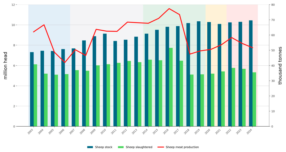
Figure 2.
Live-sheep export orientation and export-value structure in Romania, 2003–2024. (a) Live-sheep export quantity and Live Export Intensity; (b) shares of live sheep and sheep meat in their combined export value. The dashed line marks the 50% predominance threshold used for H1.
Figure 2.
Live-sheep export orientation and export-value structure in Romania, 2003–2024. (a) Live-sheep export quantity and Live Export Intensity; (b) shares of live sheep and sheep meat in their combined export value. The dashed line marks the 50% predominance threshold used for H1.
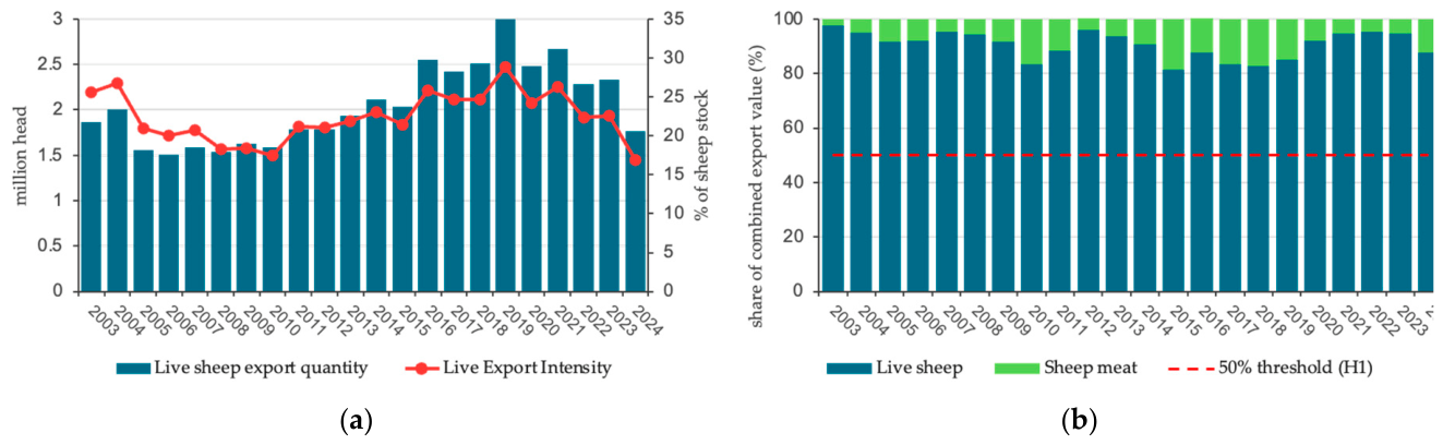
Figure 3.
Export values and export unit values for Romanian live sheep and sheep meat, 2003–2024. (a) Nominal export values; (b) Live Export Unit Value expressed in USD/head and Sheep Meat Export Unit Value expressed in USD/kg. Shaded areas correspond to the five analytical periods defined in Section 2.6. The two unit-value series use different measurement units and should not be interpreted as directly comparable product prices.
Figure 3.
Export values and export unit values for Romanian live sheep and sheep meat, 2003–2024. (a) Nominal export values; (b) Live Export Unit Value expressed in USD/head and Sheep Meat Export Unit Value expressed in USD/kg. Shaded areas correspond to the five analytical periods defined in Section 2.6. The two unit-value series use different measurement units and should not be interpreted as directly comparable product prices.
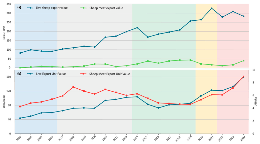
Figure 4.
Export-market concentration and partner diversification in the Romanian sheep sector, 2003–2024. (a) Herfindahl–Hirschman Index for live sheep and sheep meat exports; (b) Number of Export Partners. The dashed line indicates the HHI = 0.25 threshold defined in Section 2.5. Shaded areas correspond to the five analytical periods defined in Section 2.6.
Figure 4.
Export-market concentration and partner diversification in the Romanian sheep sector, 2003–2024. (a) Herfindahl–Hirschman Index for live sheep and sheep meat exports; (b) Number of Export Partners. The dashed line indicates the HHI = 0.25 threshold defined in Section 2.5. Shaded areas correspond to the five analytical periods defined in Section 2.6.
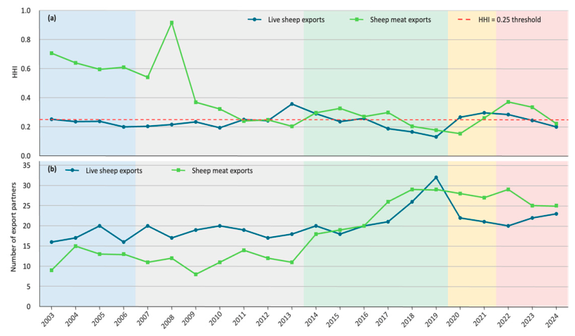
Figure 5.
Indexed mean indicators across public-policy and market-shock periods (2003–2006 = 100). (a) production-base indicators; (b) export-value and export-unit-value indicators. Period means were calculated according to Equation (20).
Figure 5.
Indexed mean indicators across public-policy and market-shock periods (2003–2006 = 100). (a) production-base indicators; (b) export-value and export-unit-value indicators. Period means were calculated according to Equation (20).
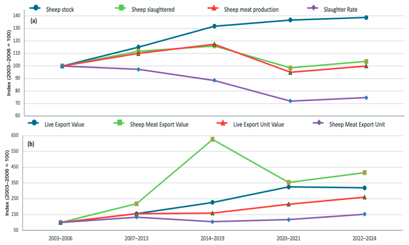
Table 1.
Coverage of commercial products included in the analysis.
| HS code | Commodity description | Analytical category |
| HS 010410 | Sheep; live | Live sheep |
| HS 020410 | Lamb carcasses and half-carcasses, fresh or chilled | Sheep meat |
| HS 020421 | Sheep carcasses and half-carcasses, excluding lamb, fresh or chilled | Sheep meat |
| HS 020422 | Sheep cuts with bone in, excluding carcasses and half-carcasses, fresh or chilled | Sheep meat |
| HS 020423 | Boneless sheep meat, fresh or chilled | Sheep meat |
| HS 020430 | Lamb carcasses and half-carcasses, frozen | Sheep meat |
| HS 020441 | Sheep carcasses and half-carcasses, excluding lamb, frozen | Sheep meat |
| HS 020442 | Sheep cuts with bone in, excluding carcasses and half-carcasses, frozen | Sheep meat |
| HS 020443 | Boneless sheep meat, frozen | Sheep meat |
| HS 020450 | Goat meat, fresh, chilled or frozen | Excluded |
Note: Descriptions have been condensed for presentation; selection and calculations used HS6 codes and full descriptions from UN Comtrade. HS 020450 was not included in the trade indicators.
Table 3.
Mean production-base indicators by analytical period.
| periodically | Sheep stock (million head) | Sheep slaughtered (million head) | Meat production (thousand t) | Slaughter rate(%) | Carcass yield(kg/head) |
| 2003–2006 | 7,449 | 5,392 | 54,883 | 72.47 | 10.17 |
| 2007–2013 | 8,565 | 6,028 | 60,326 | 70.45 | 9.97 |
| 2014–2019 | 9,812 | 6,256 | 64,438 | 64.09 | 10.25 |
| 2020–2021 | 10,184 | 5,305 | 52,065 | 52.11 | 9.81 |
| 2022–2024 | 10,330 | 5,590 | 54,853 | 54.13 | 9.81 |
Table 5.
Mean export-orientation indicators by analytical period.
| periodically | Live sheep exports (million head) | Sheep meat exports (thousand t) | Live Export Intensity(%) | Live Export Value Share(%) | Live-to-Meat ExportValue Ratio |
| 2003–2006 | 1,739 | 1,120 | 23.37 | 94.33 | 21.42 |
| 2007–2013 | 1,700 | 1,887 | 19.88 | 92.03 | 14.50 |
| 2014–2019 | 2,440 | 7,080 | 24.80 | 85.45 | 6.25 |
| 2020–2021 | 2,576 | 3,504 | 25.31 | 93.61 | 15.31 |
| 2022–2024 | 2,131 | 2,978 | 20.65 | 92.68 | 15.63 |
Table 7.
Mean export-value and export-unit-value indicators by analytical period.
| Periodically | Live export value (million USD) | Meat export value (million USD) | Live-to-Meat ExportValue Ratio | Live Export Unit Value (USD/head) | Meat Export Unit Value (USD/kg) |
| 2003–2006 | 90.87 | 5.58 | 21.42 | 52.90 | 4.85 |
| 2007–2013 | 141.03 | 12.21 | 14.50 | 81.90 | 6.50 |
| 2014–2019 | 205.92 | 34.94 | 6.25 | 84.80 | 5.08 |
| 2020–2021 | 295.41 | 19.78 | 15.31 | 114.37 | 5.72 |
| 2022–2024 | 289.86 | 23.19 | 15.63 | 137.85 | 7.39 |
Table 9.
Mean export-market concentration indicators by analytical period.
| Trade flow | periodically | NEP | CR1 (%) | CR3 (%) | CR5 (%) | HHI |
| Live sheep | 2003–2006 | 17.25 | 37.10 | 75.27 | 86.62 | 0.231 |
| Live sheep | 2007–2013 | 18.57 | 37.02 | 77.28 | 89.48 | 0.242 |
| Live sheep | 2014–2019 | 22.83 | 34.34 | 68.79 | 85.53 | 0.211 |
| Live sheep | 2020–2021 | 21.50 | 41.23 | 82.87 | 92.19 | 0.280 |
| Live sheep | 2022–2024 | 21.67 | 38.51 | 76.81 | 87.62 | 0.242 |
| Sheep meat | 2003–2006 | 12.50 | 76.49 | 99.43 | 99.80 | 0.637 |
| Sheep meat | 2007–2013 | 11.29 | 49.52 | 89.54 | 96.97 | 0.406 |
| Sheep meat | 2014–2019 | 23.50 | 41.30 | 78.10 | 87.96 | 0.262 |
| Sheep meat | 2020–2021 | 27.50 | 36.59 | 65.36 | 78.12 | 0.206 |
| Sheep meat | 2022–2024 | 26.33 | 48.88 | 75.85 | 85.92 | 0.309 |
Table 11.
Permutation Kruskal–Wallis tests for differences across the five analytical periods.
| Indicator | N | H | Permutation p | Adjusted p | η²H | Conclusion |
| Live Export Value | 22 | 18,449 | <0.001 | <0.001 | 0.850 | Significant |
| Sheep Meat Export Value | 22 | 15,365 | <0.001 | <0.001 | 0.669 | Significant |
| Live Value Share | 22 | 9,689 | 0.025 | 0.045 | 0.335 | Significant |
| Live Export Unit Value | 22 | 16,671 | <0.001 | <0.001 | 0.745 | Significant |
| Sheep Meat Export Unit Value | 22 | 13,426 | <0.001 | 0.002 | 0.554 | Significant |
| Live Export HHI | 22 | 4,252 | 0.399 | 0.466 | 0.015 | Not significant |
| Live Export CR3 | 22 | 6,008 | 0.198 | 0.252 | 0.118 | Not significant |
| Sheep Meat Export HHI | 22 | 10,161 | 0.019 | 0.039 | 0.362 | Significant |
| Sheep Meat Export CR3 | 22 | 13,940 | <0.001 | 0.002 | 0.585 | Significant |
| Sheep Stock | 22 | 18,316 | <0.001 | <0.001 | 0.842 | Significant |
| Sheep Slaughtered | 22 | 6,279 | 0.175 | 0.245 | 0.134 | Not significant |
| Sheep Meat Production | 22 | 3,392 | 0.535 | 0.576 | 0.000 | Not significant |
| Slaughter Rate | 22 | 8,464 | 0.054 | 0.084 | 0.263 | Not significant |
| Carcass Yield | 22 | 1,276 | 0.886 | 0.886 | 0.000 | Not significant |
Notes: Period differences were tested using permutation Kruskal–Wallis tests. Adjusted p-values were obtained with the Benjamini–Hochberg procedure across the family of 14 comparisons. η²H was calculated according to Equation (25); negative sample estimates were reported as zero because they indicated no detectable effect. Statistical significance was assessed at adjusted p < 0.05.
Table 12.
Integrated hypothesis-testing results.
| H | Tested proposition | Primary test | Statistical evidence | Decision |
| H1 | Predominance of live-animal exports | One-sided exact sign test | 22/22 years with Live Value Share > 0.50; median = 0.922; p < 0.001 | Supported |
| H2 | Differences across policies and shock periods | 14 permutation Kruskal–Wallis tests; BH correction | 8/14 adjusted significant tests; strongest effects for Live Export Value, Sheep Stock and Live Export Unit Value | Partially supported |
| H3 | Geographical concentration of export markets | One-sided one-sample Wilcoxon versus HHI = 0.25 | Live: median = 0.237, W = 74.0, p = 0.957; meat: median = 0.311, W = 205.0, p = 0.005 | Partially supported |
| H4 | Live export value exceeds sheep-meat export value | One-sided paired Wilcoxon signed-rank test | W = 253.0; p < 0.001; median live-to-meat ratio = 11.81; rrb = 1,000 | Supported |
Note: BH = Benjamini–Hochberg; HHI = Herfindahl–Hirschman Index; rrb = rank-biserial correlation calculated according to Equation (26). Statistical significance was assessed at p < 0.05.
Disclaimer/Publisher’s Note: The statements, opinions and data contained in all publications are solely those of the individual author(s) and contributor(s) and not of MDPI and/or the editor(s). MDPI and/or the editor(s) disclaim responsibility for any injury to people or property resulting from any ideas, methods, instructions or products referred to in the content. |
© 2026 by the authors. Licensee MDPI, Basel, Switzerland. This article is an open access article distributed under the terms and conditions of the Creative Commons Attribution (CC BY) license (http://creativecommons.org/licenses/by/4.0/).
Copyright: This open access article is published under a Creative Commons CC BY 4.0 license, which permit the free download, distribution, and reuse, provided that the author and preprint are cited in any reuse.