Dual-Axis Structure of the Uncertainty Principle: No-Common-Reduction and a Total-Variance Bound

1. Introduction

In 1927, Heisenberg used the microscope thought experiment to expose a trade-off between spatial resolution and momentum disturbance [1]. Kennard soon established the standard-deviation relation for position and momentum [2]. Robertson extended the result to an arbitrary pair of self-adjoint operators [3], and Schrödinger added the covariance term that completes the variance inequality [4]. The resulting uncertainty relations are not empirical approximations. They follow rigorously from positivity of the Hilbert-space inner product and from operator noncommutativity.

The word uncertainty, nevertheless, is used for physically distinct propositions. It may refer to the statistical spreads of two quantities in one preparation, to the accuracy limits of a joint measurement, or to the disturbance of a later measurement by an earlier one. Ozawa’s universally valid error–disturbance relation and subsequent measurement theory demonstrate that preparation uncertainty cannot be identified with error and disturbance [5,6]. The foundation of $\Delta Q\Delta P\ge \hslash /2$ is therefore not the claim that a position measurement mechanically “kicks” the particle. The variance relation holds in the prepared state even when no prior measurement has occurred.

This distinction leaves open a question about the formation of empirical facts. An experiment does not return a value detached from its conditions; it returns a record formed in a definite state of the observer system. The PhysObser Axiom expresses this fact-generating structure through two irreducible coordinates: a physical state and a physically instantiated observational state,

$$\iota :\mathcal{B}\hookrightarrow \mathcal{X}\times \mathcal{S},R:\mathcal{B}⟶\mathcal{O},r=R(x,s).$$

(1)

Here s is the objective state of the observer system. It is neither consciousness nor a synonym for instrumental noise. A fact arises where the two axes meet. A single-axis description is adequate only if s can be eliminated without changing the feasible domain, the conditional responses, or the composition of transport.

The uncertainty principle can now be asked in a different form: can position facts and momentum facts be compressed simultaneously into two sharp coordinates on one physical axis? This paper gives three connected answers. First, after an explicit quantum closure, the two fact interfaces pull back to self-adjoint operators on a joint space. Zero variance requires common eigensupport, while a nonzero central commutator excludes such support. Second, when the observational state becomes a readable classical register, fibrewise quantum spread and the variation of conditional means along the observational axis jointly determine the total uncertainty. These contributions enter a single product bound rather than remaining separate terms in a variance decomposition. Third, when fact observables generate covariant transport in physical and observational directions, the mixed curvature enters both their commutator and their uncertainty bound.

The derivation follows the chain

$$\begin{array}{cc}\hfill \mathrm{dual}-\mathrm{axis}\mathrm{fact}\mathrm{formation}& ⟶\mathrm{quantum}\mathrm{fact}\mathrm{operators},\hfill \\ \hfill & ⟶\mathrm{fibrewise}\mathrm{and}\mathrm{total}-\mathrm{variance}\mathrm{bounds},\hfill \\ \hfill & ⟶\mathrm{curvature}\mathrm{form}.\hfill \end{array}$$

(2)

The dual-axis structure explains why uncertainty belongs to an obstruction among fact interfaces. Complex Hilbert structure, positivity, and projective-unitary transport supply the quantum closure. The central scale of the Weyl cocycle finally fixes ℏ. These levels unfold along one argument while retaining their distinct logical roles.

2. The PhysObser Axiom and the Fact Interface

2.1. The Dual-Axis Premise

The PhysObser Axiom is the starting point of the present argument. Its consequence for quantum uncertainty, rather than its independent foundation, is the subject of this paper.

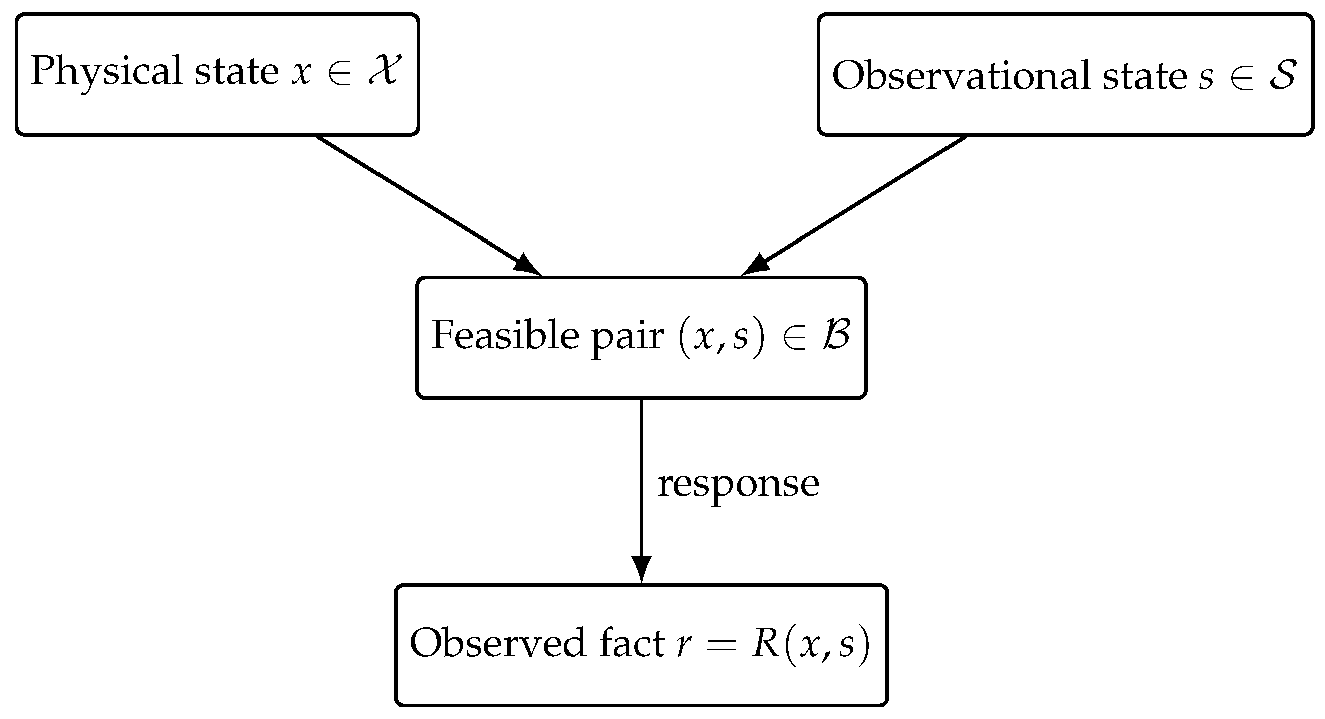
PhysObser Axiom 1 (Physical–observational dual-axis structure)An empirical fact is jointly generated by a physical state $x\in \mathcal{X}$ and a physically instantiated observational state $s\in \mathcal{S}$. Its domain is a feasible typed relation and its response is

$$\iota :\mathcal{B}\hookrightarrow \mathcal{X}\times \mathcal{S},R:\mathcal{B}⟶\mathcal{O},r=R(x,s).$$

(3)

Neither coordinate is in general reducible to the other without loss of fact-forming distinctions.

Here $\mathcal{X}$ is the physical-state space, while $\mathcal{S}$ is the state space of the observer system. The latter denotes neither consciousness nor instrumental noise. The feasible relation $\mathcal{B}$ need not fill $\mathcal{X}\times \mathcal{S}$: it records which physical and observational states can coexist in a fact-forming event. The response space $\mathcal{O}$ may contain deterministic records or probability laws. Thus $\mathcal{B}$ answers which pairings can occur, whereas R answers what fact an admissible pairing forms.

For fixed s, $R_s\left(x\right)=R(x,s)$ is a conditional fact on the physical axis. For fixed x, $R_x\left(s\right)=R(x,s)$ follows one physical state across observational states. These sections induce the conditional equivalences

$$\begin{array}{cc}\hfill x_1{\sim }_s{x}_2& \iff R(x_1,s)=R(x_2,s),\hfill \end{array}$$

(4)

$$\begin{array}{cc}\hfill s_1{\sim }_x{s}_2& \iff R(x,s_1)=R(x,s_2).\hfill \end{array}$$

(5)

The first identifies physical differences unresolved at s; the second identifies observational differences to which x is insensitive. These are response-dependent equivalences, not definitions of the two axes themselves.

The relevance to uncertainty is now immediate but not yet quantitative. A fact associated with A is formed on an observational section $s_A$; a fact associated with B is formed on a section $s_B$. Treating both as simultaneously sharp properties of x alone amounts to replacing these two interfaces by one common sharp section over the physical axis. The PhysObser Axiom identifies what such a reduction would have to erase. Quantum closure will determine whether the reduction is mathematically possible.

Figure 1. A fact is not read from the physical axis alone. It is formed on a feasible physical–observational pairing.

Figure 1. A fact is not read from the physical axis alone. It is formed on a feasible physical–observational pairing.

2.2. The Comparison Problem

Once s is allowed to vary, the conditional facts $R_s$ belong to different observational sections. Comparing them requires a rule for carrying fact descriptions from one section to another. The PhysObser Axiom makes this problem unavoidable without yet selecting a Hilbert space, a unitary transport law, a connection, or a quantum of action. The dual-axis premise poses the problem; quantum closure gives it a specifically quantum answer.

3. Quantum Closure and Joint Fact Operators

3.1. Additional Closure Conditions

To reach quantum uncertainty relations, the following closure conditions are added to the dual-axis structure:

1.

Every admissible observational fibre carries a complex Hilbert space, and the joint system is represented by ${\mathcal{H}}_{\mathrm{PO}}$. In a separable realization one may take ${\mathcal{H}}_{\mathrm{PO}}={\mathcal{H}}_{\mathrm{P}}\otimes {\mathcal{H}}_{\mathrm{O}}$.

2.

A joint state is a positive trace-one operator ${\rho }_{\mathrm{PO}}$, and outcome statistics are described by positive-operator-valued measures.

3.

Reversible fibre comparisons preserve probability pairings and are therefore implemented by unitary or projective-unitary transport.

4.

Sharp fact quantities are represented by self-adjoint operators on appropriate domains in ${\mathcal{H}}_{\mathrm{PO}}$.

The PhysObser Axiom concerns the formation of facts. These conditions add the complex linearity, positivity, and reversible transport that distinguish a quantum theory of facts.

3.2. Quantum Comparison and Mixed Curvature

Under the third closure condition, observational fibres are compared by unitary maps

$$U(s_2\leftarrow s_1):{\mathcal{H}}_{s_1}⟶{\mathcal{H}}_{s_2}.$$

(6)

On a smooth region of $\mathcal{B}$ where the physical and observational projections define complementary local directions, consistent comparison induces a connection. With the Hermitian convention used here,

$$\nabla =\mathrm{d}-i\mathcal{A},\mathcal{A}={\mathcal{A}}_{\mathcal{X}}+{\mathcal{A}}_{\mathcal{S}}.$$

(7)

Its curvature is

$$\mathcal{F}=\mathrm{d}\mathcal{A}-i\mathcal{A}\wedge \mathcal{A}={\mathcal{F}}_{\mathcal{X}\mathcal{X}}+{\mathcal{F}}_{\mathcal{X}\mathcal{S}}+{\mathcal{F}}_{\mathcal{S}\mathcal{S}}.$$

(8)

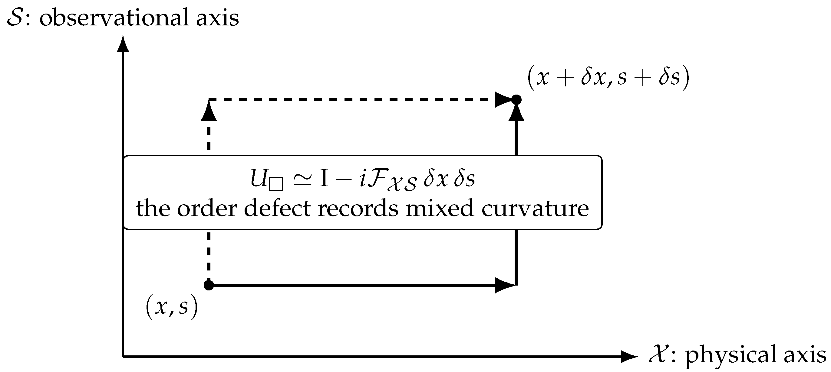
The mixed component ${\mathcal{F}}_{\mathcal{X}\mathcal{S}}$ measures the order defect between changing the physical state and changing the observational state. Around an infinitesimal mixed loop $\square (u,v)$,

$$U_{\square }=\mathrm{I}-i\mathcal{F}(u,v)\delta x\delta s+O\left({\parallel (\delta x,\delta s)\parallel }^3\right).$$

(9)

The two-axis structure first makes comparison necessary. Once comparison is unitary and smooth, a connection follows; when the two orders of transport fail to agree, their residual is curvature.

3.3. Joint Fact Operators

If an observational interface is implemented by a joint unitary $V_A$ and an observational pointer $M_A$, its fact operator pulled back to a common initial section is

$$\mathbb{A}=V_A^{†}({\mathrm{I}}_{\mathrm{P}}\otimes M_A)V_A.$$

(10)

A second interface similarly gives $\mathbb{B}$. Equation (10) does not demote the observational state to instrumental error. Rather, it places the object, the observational state, and their coupling in the same joint space. An ideal measurement merely makes $\mathbb{A}$ reproduce the statistics of $A\otimes {\mathrm{I}}_{\mathrm{O}}$ on a specified preparation subspace.

For the joint state $\rho ={\rho }_{\mathrm{PO}}$, define

$$\begin{array}{cc}\hfill {\langle \mathbb{A}\rangle }_{\rho }& =Tr\left(\rho \mathbb{A}\right),\hfill \end{array}$$

(11)

$$\begin{array}{cc}\hfill {\left({\Delta }_{\rho }\mathbb{A}\right)}^2& =Tr\left[\rho {(\mathbb{A}-{\langle \mathbb{A}\rangle }_{\rho })}^2\right].\hfill \end{array}$$

(12)

This variance belongs to the joint statistics of an already formed fact. It should not be assigned in advance wholly to either axis.

3.4. The Uncertainty Theorem on the Joint Space

Theorem 1 

(Robertson–Schrödinger relation for joint facts). Let $\mathbb{A}$ and $\mathbb{B}$ be bounded self-adjoint fact operators on ${\mathcal{H}}_{\mathrm{PO}}$. For every density operator ρ,

$$\begin{array}{cc}\hfill {\left({\Delta }_{\rho }\mathbb{A}\right)}^2{\left({\Delta }_{\rho }\mathbb{B}\right)}^2\ge & {\displaystyle \frac{1}{4}}{\left|Tr\left(\rho [\mathbb{A},\mathbb{B}]\right)\right|}^2\hfill \\ \hfill & +{\displaystyle \frac{1}{4}}{\left|Tr\left(\rho \{\delta \mathbb{A},\delta \mathbb{B}\}\right)\right|}^2,\hfill \end{array}$$

(13)

where $\delta \mathbb{A}=\mathbb{A}-{\langle \mathbb{A}\rangle }_{\rho }$ and $\delta \mathbb{B}=\mathbb{B}-{\langle \mathbb{B}\rangle }_{\rho }$. For unbounded operators, the same conclusion holds on a common dense domain on which all second moments and the relevant product quadratic forms are defined.

Proof. 

First let $\rho =|\Psi \rangle \langle \Psi |$ and set

$$|u\rangle =\delta \mathbb{A}|\Psi \rangle ,|v\rangle =\delta \mathbb{B}|\Psi \rangle .$$

(14)

The Cauchy–Schwarz inequality gives

$${\left(\Delta \mathbb{A}\right)}^2{\left(\Delta \mathbb{B}\right)}^2=\langle u|u\rangle \langle v|v\rangle \ge {\left|\langle u|v\rangle \right|}^2.$$

(15)

Moreover,

$$\begin{array}{cc}\hfill \Re \langle u|v\rangle & ={\displaystyle \frac{1}{2}}\langle \{\delta \mathbb{A},\delta \mathbb{B}\}\rangle ,\hfill \end{array}$$

(16)

$$\begin{array}{cc}\hfill \Im \langle u|v\rangle & ={\displaystyle \frac{1}{2i}}\langle [\mathbb{A},\mathbb{B}]\rangle .\hfill \end{array}$$

(17)

Adding the squares of the real and imaginary parts proves Eq. (13). For a mixed state, take $u=\delta \mathbb{A}\sqrt{\rho }$ and $v=\delta \mathbb{B}\sqrt{\rho }$ in Hilbert–Schmidt space and apply Cauchy–Schwarz once more. □

Dropping the nonnegative covariance term gives the Robertson form

$${\Delta }_{\rho }\mathbb{A}{\Delta }_{\rho }\mathbb{B}\ge {\displaystyle \frac{1}{2}}\left|{\langle [\mathbb{A},\mathbb{B}]\rangle }_{\rho }\right|.$$

(18)

The formula is identical to the standard quantum relation, but its mathematical setting is different. Here $\mathbb{A}$ and $\mathbb{B}$ are operators pulled back from two fact interfaces to the joint physical–observational space. They are not postulated as properties suspended on the physical axis independently of observational state.

4. The No-Common-Reduction Theorem

4.1. A Necessary Condition for Jointly Exact Facts

Definition 2 

(Common sharpening). For a normalized state $|\Psi \rangle$, two facts arejointly sharp in the stateif ${\Delta }_{\Psi }\mathbb{A}={\Delta }_{\Psi }\mathbb{B}=0$. They possess acommon sharp section on a closed subspace Kif there is a joint projection-valued measure whose marginals are the spectral measures of ${\mathbb{A}|}_K$ and ${\mathbb{B}|}_K$. The former is state-dependent; the latter is a uniform statement on a subspace.

Theorem 2 

(No common single-axis reduction). Let $\mathbb{A}$ and $\mathbb{B}$ be self-adjoint fact operators, and let

$${\mathcal{D}}_{AB}:=Dom\left(\mathbb{A}\mathbb{B}\right)\cap Dom\left(\mathbb{B}\mathbb{A}\right).$$

(19)

If a normalized vector $|\Psi \rangle \in {\mathcal{D}}_{AB}$ makes the two facts jointly sharp,

$${\Delta }_{\Psi }\mathbb{A}=0,{\Delta }_{\Psi }\mathbb{B}=0,$$

(20)

then $|\Psi \rangle$ is a common eigenstate and

$$\langle \Psi \left|\right[\mathbb{A},\mathbb{B}\left]\right|\Psi \rangle =0.$$

(21)

Suppose further that a nonzero closed subspace K reduces both operators. Define

$${\mathcal{D}}_K:=K\cap {\mathcal{D}}_{AB},$$

(22)

and assume that ${\mathcal{D}}_K$ is dense in K and that, on ${\mathcal{D}}_K$,

$$[\mathbb{A},\mathbb{B}]{|}_{{\mathcal{D}}_K}=ic{\mathrm{I}}_{{\mathcal{D}}_K},c\ne 0.$$

(23)

Then no normalized vector in ${\mathcal{D}}_K$ makes the two facts jointly sharp.

Proof. 

The equality ${\Delta }_{\Psi }\mathbb{A}=0$ is equivalent to

$${\parallel (\mathbb{A}-\langle \mathbb{A}\rangle )|\Psi \rangle \parallel }^2=0,$$

(24)

and hence $\mathbb{A}|\Psi \rangle =a|\Psi \rangle$. Likewise, $\mathbb{B}|\Psi \rangle =b|\Psi \rangle$. Because $|\Psi \rangle \in {\mathcal{D}}_{AB}$, both products are defined, and $\langle \Psi \left|\mathbb{A}\mathbb{B}\right|\Psi \rangle =ab$ while $\langle \Psi \left|\mathbb{B}\mathbb{A}\right|\Psi \rangle =ba$. This proves Eq. (21). If $|\Psi \rangle \in {\mathcal{D}}_K$ and Eq. (23) holds, the same expectation value equals $ic\ne 0$, a contradiction. □

The theorem turns “impossibility of simultaneous exactness” into a support statement on the dual-axis space. Sharpening fact A belongs to the fibre selected by an observational state $s_A$; sharpening fact B belongs to the fibre selected by $s_B$. If these local sharpenings could be assembled into one section, they would require common eigensupport. A nonzero central commutator prevents precisely this assembly.

Proposition 1 

(Criterion for a common sharp measure). Let $P^A$ and $P^B$ be the spectral measures of two self-adjoint fact operators. A joint projection-valued measure with marginals $P^A$ and $P^B$ exists if and only if every pair of spectral projections commutes:

$$[P^A\left(\Delta \right),P^B\left(\Gamma \right)]=0\mathrm{for}\mathrm{all}\mathrm{Borel}\mathrm{sets}\Delta ,\Gamma .$$

(25)

Proof. 

If a joint projection-valued measure G exists, then

$$P^A\left(\Delta \right)=G(\Delta \times \mathbb{R}),P^B\left(\Gamma \right)=G(\mathbb{R}\times \Gamma ).$$

(26)

Projections in the range of one projection-valued measure commute, and $P^A\left(\Delta \right)P^B\left(\Gamma \right)=G(\Delta \times \Gamma )$; hence Eq. (25). Conversely, if all spectral projections commute, define

$$G(\Delta \times \Gamma )=P^A\left(\Delta \right)P^B\left(\Gamma \right)$$

(27)

on measurable rectangles. Countable additivity and the standard extension theorem for commuting spectral measures give a unique projection-valued measure on the product Borel $\sigma$-algebra, with marginals $P^A$ and $P^B$. □

Noncommutativity therefore does not indicate simultaneous values that remain to be supplied; it is the operator criterion for the absence of a common sharp fact space. In particular, Eq. (23) prevents ${\mathbb{A}|}_K$ and ${\mathbb{B}|}_K$ from commuting, and Proposition 1 excludes a common sharp section on K. This conclusion concerns sharp observables. Unsharp POVMs can be measured jointly at the price of added noise, subject to a different class of error and joint-measurability bounds [6].

4.2. Position and Momentum

Under canonical quantum closure,

$$[Q,P]=i\hslash \mathrm{I}.$$

(28)

Restricting the joint fact operators $\mathbb{Q}$ and $\mathbb{P}$ to an ideal-measurement preparation subspace, and requiring them to reproduce the statistics of Q and P, Eq. (18) immediately yields

$$\Delta Q\Delta P\ge {\displaystyle \frac{\hslash }{2}}.$$

(29)

In dual-axis language, Eq. (29) does not say that a particle was merely “blurred” before measurement, nor that the experimenter lacked information. It says that the position-fact interface and the momentum-fact interface cannot both be compressed into two sharp coordinates on one physical axis. The observational state is neither an observer’s consciousness nor instrumental noise. It is an objective state coordinate that co-occurs with the physical state in fact formation and can be controlled and compared.

4.3. Physical Meaning of the Dual-Axis Reading

For one physical preparation x, position and momentum facts are formed through different conditional interfaces,

$$(x,s_Q)⟼R_Q(x,s_Q),(x,s_P)⟼R_P(x,s_P).$$

(30)

Sharpness is defined within each interface. To assert simultaneous exactness, however, is to demand more: after both interfaces are pulled back to a common preparation space, their spectral measures must be marginals of one sharp measure. Proposition 1 shows that this is possible exactly when the corresponding spectral projections commute. The canonical commutator excludes that common section.

The uncertainty product therefore measures a failure of common reduction. It is not produced by ignorance of x, by a fluctuating observer, or by an unavoidable mechanical disturbance during readout. Even with a perfectly specified physical preparation and a calibrated observational state, the two fact interfaces remain noncommutative. What cannot be made exact is not either local interface by itself, but their proposed identification as two simultaneously sharp coordinates of one observationally independent physical description.

The constant $\hslash /2$ adds the quantitative scale. The PhysObser Axiom supplies the two-axis grammar of fact formation; Hilbert-space positivity converts incompatibility into a variance bound; and the central normalization of the Weyl relation fixes the elementary action scale. The physical meaning and the numerical magnitude of the uncertainty relation therefore arise at different, consecutive levels of the argument.

5. How Variance Decomposes Across the Two Axes

5.1. A Classicalized Observational Register

When observational states have decohered into a distinguishable classical register, let $(\mathcal{S},\Sigma ,\nu )$ be a probability space and ${\left\{{\mathcal{H}}_s\right\}}_{s\in \mathcal{S}}$ a measurable field of Hilbert spaces. The appropriate algebra of block-diagonal observables is the decomposable von Neumann algebra

$$\mathfrak{M}={\int }_{\mathcal{S}}^{\oplus }\mathcal{B}\left({\mathcal{H}}_s\right)\mathrm{d}\nu \left(s\right)\mathrm{on}{\mathcal{H}}_{\mathrm{PO}}={\int }_{\mathcal{S}}^{\oplus }{\mathcal{H}}_s\mathrm{d}\nu \left(s\right).$$

(31)

Let $s\mapsto {\rho }_s$ be a measurable field of positive trace-class operators with $Tr{\rho }_s=1$ almost everywhere. It defines the normal state

$$\omega \left(X\right)={\int }_{\mathcal{S}}Tr\left({\rho }_s{X}_s\right)\mathrm{d}\nu \left(s\right),X={\int }_{\mathcal{S}}^{\oplus }{X}_s\mathrm{d}\nu \left(s\right)\in \mathfrak{M}.$$

(32)

The functional extends by monotone convergence to positive operators affiliated with $\mathfrak{M}$. We write ${\mathbb{E}}_S\left[f\left(S\right)\right]={\int }_{\mathcal{S}}f\left(s\right)\mathrm{d}\nu \left(s\right)$ and use ${Var}_S$ for variance with respect to $\nu$. For a discrete or countable register, Eq. (32) is equivalent to the familiar density operator ${⨁}_s{p}_s{\rho }_s$. Unlike a decomposable density-operator formula, it remains valid for a non-atomic register.

Let the fact observables be self-adjoint decomposable operators affiliated with $\mathfrak{M}$,

$$\mathbb{A}={\int }_{\mathcal{S}}^{\oplus }{A}_s\mathrm{d}\nu \left(s\right),\mathbb{B}={\int }_{\mathcal{S}}^{\oplus }{B}_s\mathrm{d}\nu \left(s\right),$$

(33)

and assume throughout this section that the required second moments are finite. Write

$$m_A\left(s\right)=Tr\left({\rho }_s{A}_s\right),v_A\left(s\right)=Tr\left[{\rho }_s{(A_s-m_A\left(s\right))}^2\right].$$

(34)

Proposition 2 

(Dual-axis law of total variance). Under Eq. (33), the variance of the joint fact decomposes exactly as

$${Var}_{\omega }\left(\mathbb{A}\right)={\mathbb{E}}_S\left[v_A\left(S\right)\right]+{Var}_S\left[m_A\left(S\right)\right].$$

(35)

Proof. 

Equations (32) and (33) give

$$\omega \left({\mathbb{A}}^2\right)=\int Tr\left({\rho }_s{A}_s^2\right)\mathrm{d}\nu \left(s\right)={\mathbb{E}}_S[v_A\left(S\right)+m_A{\left(S\right)}^2].$$

(36)

Subtracting $\omega {\left(\mathbb{A}\right)}^2={\mathbb{E}}_S{\left[m_A\left(S\right)\right]}^2$ proves Eq. (35). □

Define $m_B\left(s\right)$ and $v_B\left(s\right)$ analogously. On each observational fibre, let

$$\begin{array}{cccc}\hfill \delta A_s& =A_s-m_A\left(s\right){\mathrm{I}}_s,\hfill & \hfill \delta B_s& =B_s-m_B\left(s\right){\mathrm{I}}_s,\hfill \end{array}$$

(37)

$$\begin{array}{cccc}\hfill c\left(s\right)& ={\displaystyle \frac{1}{2i}}Tr\left({\rho }_s[A_s,B_s]\right),\hfill & \hfill k\left(s\right)& ={\displaystyle \frac{1}{2}}Tr\left({\rho }_s\{\delta A_s,\delta B_s\}\right),\hfill \end{array}$$

(38)

and set

$$\chi \left(s\right)=\sqrt{c{\left(s\right)}^2+k{\left(s\right)}^2}.$$

(39)

Both $c\left(s\right)$ and $k\left(s\right)$ are real. The fibrewise Robertson–Schrödinger relation is

$$v_A\left(s\right)v_B\left(s\right)\ge \chi {\left(s\right)}^2\mathrm{for}\mathrm{almost}\mathrm{every}s.$$

(40)

Theorem 3 

(Dual-axis total uncertainty). Let $s\mapsto ({\rho }_s,A_s,B_s)$ be a measurable field as above, with $A_s$ and $B_s$ self-adjoint almost everywhere. Assume that the conditional commutator and anticommutator forms are defined on the support of ${\rho }_s$, and that all quantities appearing below are integrable. Then

$${\Delta }_{\omega }\mathbb{A}{\Delta }_{\omega }\mathbb{B}\ge {\mathbb{E}}_S\left[\chi \left(S\right)\right]+\sqrt{{Var}_S\left[m_A\left(S\right)\right]{Var}_S\left[m_B\left(S\right)\right]}.$$

(41)

Proof. 

Put

$$a={\mathbb{E}}_S\left[v_A\left(S\right)\right],b={Var}_S\left[m_A\left(S\right)\right],c={\mathbb{E}}_S\left[v_B\left(S\right)\right],d={Var}_S\left[m_B\left(S\right)\right].$$

The total-variance identity gives

$${\Delta }_{\omega }\mathbb{A}{\Delta }_{\omega }\mathbb{B}=\sqrt{(a+b)(c+d)}.$$

(42)

Because $a,b,c,d\ge 0$,

$$(a+b)(c+d)-{(\sqrt{ac}+\sqrt{bd})}^2={(\sqrt{ad}-\sqrt{bc})}^2\ge 0,$$

(43)

and therefore

$$\sqrt{(a+b)(c+d)}\ge \sqrt{ac}+\sqrt{bd}.$$

(44)

The Cauchy–Schwarz inequality and Eq. (40) further imply

$$\sqrt{ac}\ge {\mathbb{E}}_S\left[\sqrt{v_A\left(S\right)v_B\left(S\right)}\right]\ge {\mathbb{E}}_S\left[\chi \left(S\right)\right].$$

(45)

Combining Eqs. (44) and (45) proves Eq. (41). □

The inequality places two inequivalent sources of spread within one lower bound. The first is irreducible quantum spread inside each observational fibre. The second is the joint variation of conditional means along the observational axis. The latter is not an assumed measurement error; it is the contribution retained by aggregate statistics when $R(x,s)$ changes with s. Recording outcomes without s folds this variation into an apparent object spread. Conversely, resolving s does not remove the conditional quantum contribution.

Proposition 3 

(Equality conditions). Equality holds in Eq. (41) if and only if all of the following conditions hold:

1.

Almost every fibre saturates the Robertson–Schrödinger relation: $v_A\left(s\right)v_B\left(s\right)=\chi {\left(s\right)}^2$.

2.

The nonnegative functions $\sqrt{v_A}$ and $\sqrt{v_B}$ are linearly dependent in $L^2(\mathcal{S},\nu )$. If both ${\mathbb{E}}_S\left[v_A\right]$ and ${\mathbb{E}}_S\left[v_B\right]$ are nonzero, this is equivalent to the existence of a constant $\lambda >0$ such that $v_A\left(s\right)={\lambda }^2{v}_B\left(s\right)$ almost everywhere.

3.

Mean conditional spread and observational-axis variation have the same inter-axis ratio:

$${\mathbb{E}}_S\left[v_A\left(S\right)\right]{Var}_S\left[m_B\left(S\right)\right]={\mathbb{E}}_S\left[v_B\left(S\right)\right]{Var}_S\left[m_A\left(S\right)\right].$$

(46)

This formulation includes degenerate zero-variance cases and requires no limiting prescription.

Proof. 

Condition 1 characterizes equality in the second inequality of Eq. (45). Condition 2 is precisely the linear-dependence condition for equality in its first, Cauchy–Schwarz, inequality. Condition 3 is equivalent to $ad=bc$, which characterizes equality in Eq. (44). The total bound is saturated exactly when all three steps are saturated. □

Corollary 1 

(Canonical conditional fibres). Suppose that, on almost every fibre, $A_s$ and $B_s$ possess a measurable common invariant core on which

$$[A_s,B_s]=i\hslash {\mathrm{I}}_s$$

(47)

holds in the quadratic-form sense, and suppose that the conditional states have finite second moments. Then

$${\Delta }_{\omega }\mathbb{A}{\Delta }_{\omega }\mathbb{B}\ge {\displaystyle \frac{\hslash }{2}}+\sqrt{{Var}_S\left[m_A\left(S\right)\right]{Var}_S\left[m_B\left(S\right)\right]}.$$

(48)

Proof. 

The canonical commutation relation gives $\left|c\right(s\left)\right|=\hslash /2$, so $\chi \left(s\right)\ge \hslash /2$. Substitution into Eq. (41) completes the proof. □

If at least one conditional mean is constant in s, Eq. (48) returns to the standard $\hslash /2$ lower bound. When both means vary with observational state, the observational-axis contribution enters the product as a nonnegative term. Aggregate single-axis statistics obscure its source; dual-axis conditional statistics separate it.

5.2. Coherent Observational States

The normal state $\omega$ describes the block-diagonal, hence classicalized, observational register. If the joint state retains coherence between distinct values of s, it is a state on the full joint algebra rather than merely on $\mathfrak{M}$; off-diagonal observables can then contribute to its moments. Equation (35) applies only after restriction to the classical register (or after decoherence in S). The joint-operator relation (13) requires no such restriction and is therefore the more general statement.

This distinction also shows why the second axis is not a renamed classical hidden variable. If s were only a classical parameter carrying every predetermined outcome, one would return to a common numerical-value assignment. The dual-axis theory instead requires an objective observational state and relations among its fibres, which may include coherence, noncommuting transport, and curvature.

6. How Mixed Curvature Enters the Uncertainty Bound

6.1. Transport-generator Theorem

Let u be a direction along the physical axis and v a direction along the observational axis, with $[u,v]=0$ in a local coordinate chart. Assume that ${\nabla }_u$ and ${\nabla }_v$ preserve a common dense core $\mathcal{D}$. Under the convention of Eq. (7), the curvature identity on $\mathcal{D}$ is

$$[{\nabla }_u,{\nabla }_v]=-i{\mathcal{F}}_{uv}.$$

(49)

On $\mathcal{D}$, define

$$G_u=-i\alpha {\nabla }_u,G_v=-i\beta {\nabla }_v,\alpha ,\beta >0,$$

(50)

and assume that these symmetric operators have self-adjoint closures, denoted by the same symbols. The boundary conditions are part of this assumption; without them a formal differential expression need not define an observable.

Theorem 4 

(Mixed-curvature uncertainty bound). Under these conditions, the commutator identity

$$[G_u,G_v]=i\alpha \beta {\mathcal{F}}_{uv},$$

(51)

holds on $\mathcal{D}$. For every normalized state $|\Psi \rangle \in \mathcal{D}$ with finite variances and a defined curvature expectation,

$${\Delta }_{\Psi }{G}_u{\Delta }_{\Psi }{G}_v\ge {\displaystyle \frac{\alpha \beta }{2}}\left|\langle \Psi \left|{\mathcal{F}}_{uv}\right|\Psi \rangle \right|.$$

(52)

Retaining the covariance term strengthens this bound according to Eq. (13).

Proof. 

Equations (50) and (49) give

$$[G_u,G_v]=(-i\alpha )(-i\beta )[{\nabla }_u,{\nabla }_v]=i\alpha \beta {\mathcal{F}}_{uv}.$$

(53)

Taking the expectation in $|\Psi \rangle$ and applying the Robertson inequality proves the result. □

Equation (52) is the direct geometric bridge between the dual-axis structure and uncertainty. When two fact quantities generate transport along different directions of the joint space, their failure to commute is the mixed curvature itself. Closed-loop holonomy and the uncertainty lower bound are then governed by the same ${\mathcal{F}}_{uv}$.

Figure 2. Two paths share the same endpoints but can yield different transports. Nonzero mixed curvature is a local obstruction to global single-axis reduction.

Figure 2. Two paths share the same endpoints but can yield different transports. Nonzero mixed curvature is a local obstruction to global single-axis reduction.

6.2. The Origin and Logical Boundary of $\hslash /2$

Equation (52) gives a general relation between curvature and uncertainty; its numerical scale is fixed only by the specific quantum closure. For canonical position and momentum, spatial translations and momentum boosts form a projective Weyl representation [7],

$$T\left(a\right)=e^{-iaP/\hslash },B\left(b\right)=e^{ibQ/\hslash },$$

(54)

with

$$T\left(a\right)B\left(b\right)=e^{-iab/\hslash }B\left(b\right)T\left(a\right).$$

(55)

Differentiating Eq. (55) near $a=b=0$ gives $[Q,P]=i\hslash \mathrm{I}$ and therefore Eq. (29). Geometrically, the exponential factor is the central holonomy of an elementary phase-space loop; its normalization supplies the minimum action scale.

Three levels must therefore be distinguished:

$$\begin{array}{cc}\hfill \mathrm{PhysObser}\mathrm{Axiom}\text{:}& \mathrm{facts}\mathrm{have}\mathrm{two}\mathrm{irreducible}\mathrm{inputs};\hfill \\ \hfill \mathrm{quantum}\mathrm{closure}\text{:}& \mathrm{fact}\mathrm{fibres}\mathrm{carry}\mathrm{complex}\mathrm{linearity}\mathrm{and}\mathrm{positivity},\hfill \\ \hfill & \mathrm{together}\mathrm{with}\mathrm{projective}-\mathrm{unitary}\mathrm{transport};\hfill \\ \hfill \mathrm{canonical}\mathrm{normalization}\text{:}& \mathrm{the}\mathrm{central}\mathrm{scale}\mathrm{of}\mathrm{the}\mathrm{Weyl}\mathrm{cocycle}\mathrm{is}\hslash .\hfill \end{array}$$

(56)

The first level explains why observational conditions cannot be removed without loss. The second generates a noncommutative fact algebra. The third fixes the exact numerical value $\hslash /2$. Without the second and third levels, the dual-axis structure alone neither derives quantum mechanics nor turns an arbitrary classical two-input system into a quantum system.

7. Relation to Established Quantum Measurement Theory

7.1. Preparation Uncertainty and Error–Disturbance Relations

The Robertson–Schrödinger relation concerns the statistical spreads of two fact quantities in one prepared state; it is already valid before measurement. Error–disturbance relations concern the measurement process itself: how accurately an interface is realized and how it changes a subsequent interface. The dual-axis structure accommodates both without identifying them. The joint state ${\rho }_{\mathrm{PO}}$ and fact operators $\mathbb{A},\mathbb{B}$ determine preparation uncertainty, whereas the couplings $V_A,V_B$ and pointer readouts determine measurement error and sequential disturbance. Thus “incompatible facts cannot be jointly sharpened” and “measuring A first changes a later measurement of B” are adjacent but distinct propositions.

7.2. Sharp and Unsharp Joint Measurements

Proposition 1 gives the complete criterion for a sharp joint measurement: two PVMs are marginals of one joint PVM exactly when their spectral projections commute. After sufficient unsharpness is introduced, incompatible observables may admit a joint POVM, at the price of reduced resolution or increased noise. Such an unsharp joint measurement does not restore the jointly exact values excluded by the canonical commutation relation; it redistributes error across a broader fact interface. The total-uncertainty bound (41) describes the sources of aggregate variance, while error–disturbance relations and POVM joint-measurability bounds constrain the quality of an interface realization. The three statements operate at different levels.

7.3. Variance and Entropic Uncertainty

Variance is not suitable for every quantum state; heavy-tailed states may have divergent second moments. Entropic uncertainty relations constrain outcome entropies through the overlap of measurement bases [8] and are more natural in such cases. The total-uncertainty theorem assumes finite second moments. Its role is to separate conditional quantum spread from observational-axis variation and then recombine them in one bound, not to replace entropic theory. Decomposing entropy along the dual axis into conditional entropy and information carried by the observational state provides a parallel direction for future development.

8. Experimental Criteria Along the Observational Axis

Equation (41) turns observational state from a background condition into a variable accessible to statistical testing. An experiment first maintains a common physical preparation while recording the observational state s together with each fact outcome. Conditional samples at fixed s estimate $m_A\left(s\right),m_B\left(s\right),v_A\left(s\right),v_B\left(s\right)$ and, where operationally accessible, $c\left(s\right),k\left(s\right)$. These quantities determine the fibrewise lower bound $\chi \left(s\right)$ and the variation along the observational axis. The aggregated data must satisfy both the total-variance identity (35) and the total-uncertainty relation (41). If marginalizing over s increases total variance and conditioning on s accounts for that increase through ${Var}_S\left[m_A\right]$ and ${Var}_S\left[m_B\right]$, the observational-axis contribution has been separated directly.

A geometric test compares orders of operation. Choose a physical direction u and an observational direction v, construct two transport paths with common endpoints, and measure the group commutator

$$W_{uv}=U_v^{-1}{U}_u^{-1}{U}_v{U}_u.$$

(57)

In the small-loop limit,

$$W_{uv}=\mathrm{I}-i{\mathcal{F}}_{uv}\delta x\delta s+O\left({\parallel (\delta x,\delta s)\parallel }^3\right).$$

(58)

The loop remainder determines ${\mathcal{F}}_{uv}$, while an independent measurement of $\Delta G_u\Delta G_v$ must satisfy Eq. (52). Statistical decomposition and closed-loop transport thus cross-check one another: the former reveals whether the observational axis enters the variance; the latter tests whether that dependence can be removed by a flat reparametrization.

If every conditional distribution and loop remainder can be absorbed simultaneously by the same reparametrization of a single x, the second axis is reducible on the experimental domain. If, for one physical path, observational-path holonomy is stable, reproducible, and obeys the composition law of transport, a single physical axis cannot supply a global fact description. The structural criterion tests whether the second axis is eliminable. A specified dual-axis action, through ${\mathcal{F}}_{\mathcal{X}\mathcal{S}}(x,s)$ or a parameter-free invariant, must then provide the numerical discrimination among competing dynamical theories.

9. Discussion

9.1. Uncertainty Is Not Subjective Ignorance

The observational state s is an objective state of the observer system, not a human mental state. Including it in the fact structure does not make quantum law subjective. On the contrary, what is usually grouped under the vague phrase “observational conditions” is assigned a calibratable, controllable, and transportable state position. The testable proposition is always $R(x,s)$. A detached expression $R\left(x\right)$ is valid only when s can be eliminated without loss.

9.2. The Second Axis Is Not a Classical Hidden Variable

Suppose the second axis were merely a classical variable $\lambda$ carrying predetermined results. Both facts could then be written as numerical functions $A(x,\lambda )$ and $B(x,\lambda )$, so the theory would still presuppose a common sharp section. Canonical noncommutativity excludes exactly this unconditional common sharpening. The dual-axis structure introduces not a hidden table of answers, but objective relations among observational fibres and the transport and curvature induced by those relations.

9.3. The Structural Meaning of Uncertainty

Single-axis language often asks, “Why can a particle not possess an exact position and an exact momentum at once?” The dual-axis structure changes the grammar of the question. Position and momentum are not two numbers removed from one fact section. They are two kinds of facts formed when the physical state enters two observational interfaces. They can be compared in a joint space, yet under a nonzero central commutator they cannot be assembled into one global sharp section. The logical core is

$$\begin{array}{cc}\hfill {|}_{{\mathcal{D}}_K}=ic{\mathrm{I}}_{{\mathcal{D}}_K},c\ne 0& ⟹\mathrm{no}\mathrm{common}\mathrm{sharp}\sec \mathrm{tion}\mathrm{exists}\mathrm{on}K,\hfill \\ \hfill & ⟹\mathrm{no}\mathrm{common}\sin \mathrm{gle}-\mathrm{axis}\mathrm{reduction}.\hfill \end{array}$$

(59)

For a readable observational register, this structure gives more than a prohibition. It yields the quantitative bound

$${\Delta }_{\omega }\mathbb{A}{\Delta }_{\omega }\mathbb{B}\ge {\mathbb{E}}_S\left[\chi \left(S\right)\right]+\sqrt{{Var}_S\left[m_A\left(S\right)\right]{Var}_S\left[m_B\left(S\right)\right]}.$$

(60)

If both fact quantities generate covariant transport along dual-axis directions u and v, then $[G_u,G_v]=i\alpha \beta {\mathcal{F}}_{uv}$. Algebraic incompatibility and geometric holonomy are expressed by the same mixed curvature. A nonzero curvature operator may have zero expectation in a particular state; in that case the covariance term in Eq. (13), or higher-order and state-independent relations, may still impose nontrivial constraints. The Robertson bound contains the curvature expectation, not a state-free sign test.

10. Conclusions

The PhysObser Axiom places facts on $\mathcal{B}\hookrightarrow \mathcal{X}\times \mathcal{S}$, where $R(x,s)$ is jointly generated by a physical state and a physically instantiated observational state. Taking this dual-axis structure as the foundational premise, the paper has derived its consequence for quantum uncertainty. Quantum closure pulls incompatible observational interfaces back to fact operators on a joint mathematical setting. Hilbert-space positivity gives the Robertson–Schrödinger relation, while a nonzero central commutator excludes a common sharp section. Position–momentum uncertainty therefore acquires a precise physical meaning: position and momentum facts cannot simultaneously be compressed into two sharp coordinates on one physical axis.

The main quantitative result is Eq. (41). It follows directly from the law of total variance and the fibrewise quantum inequality, combining conditional quantum spread with observational-axis variation in one product bound. Equation (46) and its companion conditions characterize exactly when the bound is attained. When every conditional fibre satisfies the canonical commutation relation, Eq. (48) shows that $\hslash /2$ is the irreducible fibrewise floor, while the joint variation of both conditional means adds a nonnegative contribution to the aggregate lower bound.

A connection makes different observational fibres comparable; mixed curvature converts the loop remainder of changing comparison order into the commutator of transport generators. No-common-reduction, the total-variance bound, and mixed curvature are the algebraic, statistical, and geometric expressions of the same structure. The dual-axis principle governs fact formation, quantum closure supplies a noncommutative algebra, and Weyl central normalization fixes ℏ. The resulting account is precise in both its reach and its limit: distinct fact interfaces admit consistent transport and statistical comparison, but they cannot be flattened into one physical coordinate system while their quantum structure is preserved.

References

- Heisenberg, W. Über den anschaulichen Inhalt der quantentheoretischen Kinematik und Mechanik. Z. Für Phys. vol. 43, 172–198, 1927. [CrossRef]
- Kennard, E. H. Zur Quantenmechanik einfacher Bewegungstypen. Z. Für Phys. vol. 44, 326–352, 1927. [CrossRef]
- Robertson, H. P. The Uncertainty Principle. Phys. Rev. vol. 34, 163–164, 1929. [CrossRef]
- Schrödinger, E. Zum Heisenbergschen Unschärfeprinzip. Sitzungsberichte Der Preuss. Akad. Der Wiss. Phys.-Math. Kl. 1930, 296–303. [Google Scholar]
- Ozawa, M. Universally valid reformulation of the Heisenberg uncertainty principle on noise and disturbance in measurement. Phys. Rev. A 2003, vol. 67, 042105. [Google Scholar] [CrossRef]
- Busch, P.; Lahti, P.; Werner, R. F. Colloquium: Quantum root-mean-square error and measurement uncertainty relations. Rev. Mod. Phys. 2014, vol. 86, 1261–1281. [Google Scholar] [CrossRef]
- Weyl, H. The Theory of Groups and Quantum Mechanics; Methuen: London, 1931.
- Maassen, H.; Uffink, J. B. M. Generalized entropic uncertainty relations. Phys. Rev. Lett. 1988, vol. 60, 1103–1106. [Google Scholar] [CrossRef] [PubMed]
Disclaimer/Publisher’s Note: The statements, opinions and data contained in all publications are solely those of the individual author(s) and contributor(s) and not of MDPI and/or the editor(s). MDPI and/or the editor(s) disclaim responsibility for any injury to people or property resulting from any ideas, methods, instructions or products referred to in the content. |
© 2026 by the authors. Licensee MDPI, Basel, Switzerland. This article is an open access article distributed under the terms and conditions of the Creative Commons Attribution (CC BY) license (http://creativecommons.org/licenses/by/4.0/).
Copyright: This open access article is published under a Creative Commons CC BY 4.0 license, which permit the free download, distribution, and reuse, provided that the author and preprint are cited in any reuse.