

Submitted:
07 September 2026
Posted:
08 September 2026
You are already at the latest version
Abstract
Beam Hopping (BH) technology is adopted in satellite communication systems primarily to address the rigid resource allocation issue of traditional fixed beam coverage. By dynamically adjusting beam pointing and dwell time, it achieves efficient utilization and flexible allocation of resources. This paper addresses the beam hopping scheduling problem in Low-Earth-Orbit (LEO) satellite networks for high-priority and time-sensitive services. We establish a system gain maximization model and propose a heuristic beam scheduling algorithm (HBSA) that pre-schedules critical traffic and greedily allocates remaining resources under interference and fairness constraints. We further extend the framework with a graph reinforcement learning beam-hopping scheduling scheme (GRL-BHS) that captures structural network dependencies for near-optimal adaptive scheduling. Extensive simulations against seven benchmarks demonstrate that HBSA delivers near-optimal gain (within 2% of MWC and GRL-BHS), ensures high-priority satisfaction, maintains a Jain fairness index above 0.84 under heavy load, and reduces signaling overhead by an order of magnitude, while preserving a low polynomial complexity of O(T × J × K). GRL-BHS offers the highest gain at the cost of offline training. HBSA thus emerges as the most balanced and practically deployable solution, providing a solid foundation for future intelligent BH scheduling in mega constellations.
Keywords:
beam-hopping scheduling
; Low Earth Orbit (LEO) satellite networks
; high-priority services
; time-sensitive services
; system gain maximization
; heuristic algorithm
; graph reinforcement learning
1. Introduction
In recent years, low-cost rocket launch and advanced manufacturing technology have paved the way for the deployment of satellite Internet, especially LEO satellites based. The low orbit altitude of the LEO satellite makes the space-ground transmission delay very short. It is more suitable for delay-sensitive services and application scenarios, such as multimedia entertainment, Internet of Vechile (IoV) and realtime control. LEO satellites also achieve terminal miniaturization due to the low propagation loss. At the same time, dense constellation deployment ensures seamless and global coverage. Therefore, mega LEO satellite costellation networks have been highly valued by some governments and global industry, and deployed extensively in recent years.
In satellite communication systems, the traditional fixed beam coverage mode has the problem of rigid resource allocation, which cannot flexibly adapt to the dynamic changes of business requirements in time and space. Beam Hopping (BH) technology, as a key technology for next-generation high-throughput satellites and low-orbit networks, solves this problem by dynamically adjusting beam pointing and dwell time. It has the advantages of dynamically matching business needs, improving resource utilization, reducing system costs, and being compatible with future communication technologies. The primary advantages of beam hopping technology are as follows,
- Dynamically matching business requirements. There are significant differences in communication requirements in different regions at different times. BH technology can concentrate beams in high-demand areas by perceiving real-time needs, avoiding resource waste in low-activity areas. In addition, it can quickly adjust beam allocation to cope with local traffic surges caused by temporary events (such as competitions and disasters), thereby improving system capacity.
- Improving resource utilization. Traditional fixed beams need to continuously cover all areas, resulting in scattered power. BH only activates target areas, concentrates transmission power to improve signal-to-noise ratio and spectrum efficiency, and shares frequency and power resources through time-division multiplexing, avoiding idleness caused by fixed allocation.
- Reducing system costs. Compared with multi-beam full-coverage systems, BH can replace a large number of fixed beams with a small number of reconfigurable beams using phased array antennas, reducing the hardware cost and weight of satellites. At the same time, dynamic power allocation reduces ineffective radiation and lowers energy consumption.
- Being compatible with future communication technologies. The high-speed movement of LEO satellites leads to frequent changes in coverage. BH can switch quickly to maintain continuous services, and can match the slicing and dynamic requirements of ground networks, supporting space-ground integrated resource scheduling. In addition, the pseudo-random hopping mode of BH technology enhances anti-interference capability, which is particularly important in military communications. Although it introduces challenges such as scheduling complexity, with the optimization of intelligent algorithms, BH has become a core technology driving satellite communications towards high-efficiency, intelligence, and on-demand services, laying the foundation for space-ground integrated networks.
However, in the application of high-priority and time-sensitive services, BH technology faces challenges such as delay jitter, beam switching synchronization, and increased mobility management complexity. And the challenges of beam hopping technology in high-priority and time-sensitive services are as follows,
- Delay jitter and deterministic service challenges. The beam dwell time of LEO beam-hopping networks is only at the millisecond level. The discontinuous coverage caused by beam switching leads to intermittent interruptions in traffic transmission and increased delay jitter. Coupled with the inherent long propagation delay of satellite communications, it is very challenging to meet the services with ultra-low latency QoS requirements.
- Beam switching synchronization and signaling overhead. Frequent beam switching requires strict synchronization between terminals and satellites. Signaling interactions (such as beam switching commands and channel state feedback) occupy the already limited bandwidth, thereby reducing the efficiency of effective data transmission, especially for small-packet services (such as IoT).
- Increased complexity of mobility management. High-speed moving users (such as fighter jets and high-speed rail) require more frequent beam switching, which may exceed the system switching capability, leading to an increase in link interruption probability and switching failure rate.
Existing beam hopping scheduling algorithms mostly focus on business distribution and its dynamic changes, aiming to maximize business throughput while considering user fairness, inter-beam interference suppression, and link status, but rarely take user priority and low-latency requirements into account, which limits the application capability of time-sensitive services in LEO BH satellite communication networks. Therefore, this paper proposes beam scheduling methods for high-priority and time-sensitive services in LEO satellite networks, which takes the satisfaction of high-priority and time-sensitive services as an important goal, and optimizes the beam hopping pattern while considering interference suppression, business distribution, and fairness principles.
The remainder of this paper is organized as follows. Section II reviews related work on resource management in satellite communication systems and space information networks, highlighting the gap in existing studies regarding high-priority and time-sensitive services. Section III analyzes the key influencing factors of beam hopping scheduling, including service characteristics, resource constraints, channel conditions, user mobility, and scheduling strategies. Section IV establishes the system model, defines the notation, and formulates the beam hopping scheduling problem as a system-gain maximization under constraints of fairness, interference, minimum slot allocation, and delay-guarantee for high-priority services. Section V details the proposed heuristic beam scheduling algorithm, including the computation of cell weights and costs, the determination of beam hopping intervals for time-sensitive traffic, and the beam pointing calculation, followed by an illustrative example. The details of graph-reinforcement-learning based bean scheduling approach has been proposed in Section VI. Section VII presents simulation results that evaluate the system gain, user satisfaction, Jain’s fairness index and system overhead, with a focus on quality-of-service guarantee for high-priority and time-sensitive services. Finally, Section VIII concludes the paper and discusses several directions for future work, such as adaptive beam hopping pattern design, deep reinforcement learning based distributed scheduling, and integration with advanced transmission techniques.
2. Related Works
In recent years, beam hopping scheduling for LEO satellites has become a research hotspot in the field of satellite communication. This paper reviews the existing literature, summarizes the research progress, analyzes key technologies and challenges, and investigates future development directions.
2.1. Performance Analysis of Beam-Hopping
In [1], the authors analyze uplink performance in beam-hopping satellite systems using discrete-time queueing theory. Two modes (probabilistic and deterministic) are modeled via Markov chains, deriving explicit expressions for throughput, buffer occupancy, packet loss and delay via numerical fixed-point iteration. The key findings of this paper include performance inflection points with beam resource and lower deterministic-mode delay near saturation. However, the present study acknowledges several limitations, including the reliance on ideal hopping patterns, the disregard for inter-beam interference, and the assumption that each time slot accommodates at most one packet.
2.2. Beam-Hopping with Interference Management
Sun et al. [2] proposed the energy-efficient maximal traffic satisfaction beam hopping (EEMTS-BH) strategy for geosynchronous orbit (GSO) and non-geosynchronous orbit (NGSO) coexistence scenarios, aiming to balance quality of service (QoS) and energy-efficient (EE). They decomposed the joint multi-satellite beam hopping optimization problem into four sequential sub-problems, including satellite-cell assignment and power allocation. Simulation results show this strategy outperforms existing ones in traffic satisfaction rate and energy consumption, achieving an optimal trade-off between the two key performance indicators.
The authors in [3] proposes a three-step multi-satellite beam-hopping method for NGSO systems: load balancing via mixed integer linear programming (MILP)/greedy, single-satellite pattern design using spatially isolated patterns and MILP, and inter-satellite interference avoidance by scheduling patterns with minimum distance penalty. Simulations show load gap reduction and satisfaction rate, outperforming seven benchmarks.
The letter [4] proposes a low-complexity multi-satellite beam hopping algorithm for interference mitigation under tilted beams. It models satellite-cell association (SCA) and BH slot assignment (BHSA) as a dynamic graph coloring problem and solves it via minimum-cost maximum-flow (MCMF) plus tabu search and graph coloring (joint optimization). Simulations on a 10800-satellite constellation show near-optimal performance with far lower complexity than baselines.
Paper [5] proposes throughput-driven beam hopping (TDBH) and satisfaction-rate-driven beam hopping (SDBH) for interference avoidance in integrated satellite-terrestrial networks under given interference patterns. TDBH optimizes throughput with adjustable traffic via relaxation and slot allocation; SDBH maximizes satisfaction rate via genetic algorithm with unserved-time fairness. Simulations show TDBH outperforms random scheduling; SDBH with genetic algorithm (GA) achieves average satisfaction, higher than genetic algorithm beam hopping (GABH).
Across [3-5], common limitations include fixed power allocation, plus algorithm-specific issues: exponential complexity and simplified interference ([3]), offline pre-solving ([4]), and pre-known patterns with independent scheduling ([5]). Although [2] reports no explicit drawbacks, its sequential decomposition may compromise global optimality. Collectively, these works lack adaptive power control, real-time adaptability, and mutual interference handling, calling for more integrated dynamic frameworks.
2.3. Beam-Hopping with Precoding
In [6], the authors propose an angle-based multicast user selection, beam selection, and precoding scheme for LEO satellite systems using only elevation and azimuth information, without relying on full channel state information (CSI). A low-complexity greedy algorithm and closed-form precoding are developed. Simulations show performance comparable to CSI-based methods, demonstrating robustness and feasibility for practical beam-hopping satellite communications.
A priority-based Viterbi algorithm (PBVA) has been proposed in [7] for beam hopping in LEO satellite systems with hybrid precoding, minimizing transmit power under non-uniform rate demands. Candidate snapshots are pre-filtered using inter-cell distances. Cells are prioritized by demand, and path lengths correspond to Minimum Mean Square Error (MMSE)-based precoding power. priority-based viterbi algorithm (PBVA) outperforms the greedy baseline by and approaches the lower bound within .
Jointly optimizes linear precoding, beam hopping, and DVB-S2X (Digital Video Broadcasting - Second Generation Extensions) MODCOD (MODulation and CODing) selection for GEO satellites to minimize payload power under user demand constraints has been presented in [8]. It relaxes discrete rates and sparsity via fitting and reweighted -norm, and proposes a window-based iterative algorithm. Two two-phase methods (heuristic and Deep Neuron Network (DNN)) are also provided. Simulations show power reduction.
In [9], PBVA and Priority-Based Greedy Algorithm (PBGA) for regular and irregular beam-hopping patterns in LEO satellites with hybrid precoding has been proposed, minimizing transmit power under rate constraints. Regular patterns use Viterbi on a trellis; irregular patterns use greedy allocation based on demand weights. PBVA outperforms GABH by , within of lower bound. Irregular patterns further improve by .
A dynamic beam illumination framework with selective precoding for GEO beam-hopping systems has been proposed in [10], allowing adjacent high-demand beams to be activated and precoded only when needed. Demand constraints are converted to slot counts via expectation maximization (EM)-based estimation. Three binary quadratic programming (BQP) solvers are proposed: Semi-Definition Programming (SDP) relaxation, Multiplier Penalty and Majorization-Minimization (MPMM), and greedy. Simulations show superior demand matching and lower precoding complexity than conventional BH and cluster hopping.
Despite their contributions, the reviewed works share several shortcomings. Most rely on oversimplified channel models (e.g., LOS-only, perfect or even future CSI), which are impractical for dynamic LEO environments. Traffic is typically assumed static, ignoring real-world burstiness. Computational complexity is prohibitive for many methods, particularly those based on window-based iteration or SDP/MPMM, rendering them unsuitable for onboard scheduling. Additionally, the single-user-per-cell/beam abstraction neglects intra-cell interference, and the optimality of heuristic approaches (e.g., PBGA) remains unproven. These gaps highlight the need for a low-complexity, adaptive scheme that accommodates time-varying traffic and imperfect CSI-a need that motivates our proposed framework.
2.4. Beam-Hopping with Resource Management
In [11], resource allocation in multi-beam LEO satellite integrated sensing and communications (ISAC) systems under full frequency reuse has been presented. It proposes a two-stage beam hopping method based on multi-agent actor-critic reinforcement learning. The first stage optimizes beam patterns to maximize throughput and minimize packet loss while avoiding inter-beam interference. The second stage allocates power to each beam according to traffic demand, improving resource utilization. Simulation results demonstrate effective interference avoidance, increased system throughput, reduced latency, and on-demand power allocation compared to benchmark schemes.
Paper [12] proposes low-complexity user density-based beam position design (LCUD-BPD) to minimize beam positions under a radius constraint, and low-complexity CCI-free beam hopping design (LCCF-BHD) to minimize time slots under traffic and interference constraints. LCUD-BPD iteratively finds the sparsest user and determines its best beam position (BP) via a user selection and smallest radius algorithm. Duplicated user removal further reduces BP radius. LCCF-BHD prioritizes large-radius or high-demand BPs. Simulations show near-optimal performance with complexity reduction.
Article [13] addresses dynamic beam hopping and resource allocation for NGSO satellite systems with non-uniform traffic. Using Lyapunov optimization, it minimizes a per-slot cost that includes capacity-demand gap and energy/handover penalty. The online Long-Term Joint Optimization for Beam Hopping, Bandwidth Allocation and Power Control (LO-BBP) algorithm combines matching theory (for beam hopping and bandwidth) with convex approximation (for power control). Theoretical analysis shows an trade-off between cost and queue backlog. Simulations demonstrate reduced backlog and energy versus benchmarks.
Paper [14] maximizes energy efficiency (EE) in LEO beam-hopping downlink under minimum offered-capacity-to-demand ratio (OCDR) constraints. It transforms the multi-slot problem into per-slot subproblems: power allocation (iterative Karush-Kuhn-Tucker (KKT)-based) and user selection (priority-based for EE maximization). Simulations show the proposed Energy Efficient User Selection-Energy Efficient Power Allocation (EEUS-EEPA) outperforms baselines in EE and OCDR.
In [15], authors jointly optimize beam scheduling and power allocation in LEO beam-hopping systems to minimize offered-demand mismatch. Beam scheduling is modeled as an exact potential game with Nash equilibrium reached via best-response, while power is optimized via penalty interior-point. Multiple sink nodes per beam position are considered. Simulations show joint beam scheduling and power optimization beam hopping (JBSPO-BH) outperforms greedy, round-robin, Max-SINR (Signal-to-Interference-plus-Noise Ratio), and GA-based schemes in throughput and fairness with lower complexity.
In [16], a mixed-integer linear programming (MILP) framework has been proposed to jointly optimize illumination, bandwidth, and power for LEO beam-hopping systems, minimize unserved capacity (UC), extra-served capacity (EC), and time-to-serve (TTS). A time-split variant reduces complexity by solving sequential sub-windows. Simulations show time-split MILP outperforms demand-based and genetic algorithms: UC improves by (reduced) and (enlarged), TTS halves.
The authors in [17] propose multi-satellite dynamic beam coverage-beam hopping (MSDBC-BH) for dual-layer LEO constellations, achieving two-dimensional load balancing via dynamic beam coverage (cell splitting based on traffic density) and game-matching-based cell-satellite assignment. Simulations show beam load gap reduced from to , satellite load gap reduced by , throughput improved by over Random BH (R-BH).
In [18], the authors propose an non-orthogonal multiple access (NOMA)-based collaborative beam hopping scheme for LEO satellites. It designs hopping patterns with interference threshold distance, pairs cell-edge user (CEU) with cellcenter user (CCU) into NOMA clusters using SCA-based power allocation, and applies Q-Learning for carrier selection. Simulations show NOMA outperforms timedivision multiple access (TDMA) in rate and outage probability.
In [19], the authors propose a cognitive LEO beam-hopping satellite-terrestrial network with underlay spectrum sharing. It introduces power allocation competition (PAC) for satellite pattern/power optimization, dynamic-ratio threshold (DRT) for reliable SST detection, and adaptive resource adjustment (ARA) for terrestrial CCI suppression. PAC complexity is far lower than Particle Swarm Optimization (PSO)/GA. Simulations validate QoS improvement and CCI control.
Despite these advances, several common limitations persist across the reviewed resource management schemes, include oversimplified channel models (LOS-only, static, or perfect/future CSI) and time-invariant traffic assumptions, which ignore real-world dynamics. Computational complexity is prohibitive for MILP, KKT, and game-theoretic approaches, especially in large-scale constellations. Many adopt narrow abstractions (e.g., single-user-per-cell, fixed power, single-satellite), neglecting interference and coordination. Heuristics and Q-learning lack scalability and optimality guarantees; reliance on commercial solvers, perfect CSI, or long-term statistics further hinders deployability. These gaps motivate our low-complexity, adaptive framework.
2.5. Beam-Hopping with Machine Learning
A multi-agent deep reinforcement learning (DRL) framework for joint beam pattern and bandwidth allocation in GEO beam-hopping systems has been presented in [20]. Each beam is split into two agents (illumination and bandwidth) to reduce action space. Agents share global state and reward, trained via independent DDQN. Simulations show throughput gains of over baselines and improved delay fairness. Generalization beyond training traffic range is demonstrated.
The paper [21] addresses joint power and beam scheduling in LEO satellite Internet of Things (IoT) with beam hopping. It decomposes the multi-objective problem into convex power optimization and DRL-based scheduling. The proposed action masking multiobjective double deep Q network (AMM-DDQN) uses Chebyshev scaling and action masking to handle multiple objectives and large action spaces. Simulations show real time delay reduced by over baselines, with improved throughput and fairness.
The authors in [22] propose a cooperative multi-agent Value-Decomposition Networks with Dueling Double Deep Q-Learning Network (VDN-D3QN) framework for dynamic beam hopping in LEO satellite systems with non-uniform traffic. Centralized training and distributed execution avoid inter-satellite information exchange. Each agent controls one satellite, and VDN decomposes the joint Q-value. The multi-objective reward balances throughput and delay fairness. Simulations show improved performance over baselines.
In [23], the letter proposes DeepBeam, a DRL-based joint optimization of beam-hopping scheduling and coverage control for multibeam GEO satellites. It dynamically selects each beam’s center cell and coverage radius to maximize throughput. To reduce action space, it trains a single agent and applies it to all beams with pseudo-state updates. Simulations show throughput gain and lower packet loss versus heuristics.
A two-stage satellite-terrestrial coordinated multi-satellite beam hopping framework has been proposed in [24]. Network operation control center (NOCC) solves long-term cell-satellite association via greedy+iteration to balance load; each satellite uses offline-trained QMIX (centralized training, distributed execution) for real-time traffic-driven scheduling with spatial isolation and parameter sharing. Simulations show load-gap reduction, delay reduction, average delay, and inference time.
In [25], the authors propose DeepMBS, a parameterized DRL framework for joint beam hopping (discrete) and power allocation (continuous) in multi-beam satellite systems. It extends deep Q-network (DQN) with a parameterized action space, where a policy network outputs continuous power for each discrete cell choice. An experience filtering mechanism accelerates convergence. Simulations show throughput gain and energy efficiency improvement over baselines.
A user-level dynamic beam hopping scheme for LEO satellite networks in [26], jointly optimizing beam pattern and access control based on real-time per-user traffic. A user-oriented Markov Decision Process (MDP) converts the long-term problem to short-term Q-value maximization. A deep reinforcement learning assisted enhanced genetic (DRL-EG) algorithm estimates Q-values via Sarsa and solves scheduling via enhanced genetic algorithm. Simulations show throughput and capacity gains over cell-level baselines.
The authors in [27] propose multiagent proximal policy optimization-beam pattern and resource allocation (MAPPO-BPRA) for multi-LEO satellite systems, jointly optimizing beam pattern, bandwidth, power, and precoding to maximize minimum traffic satisfaction. Each satellite is an agent with hybrid actions (discrete beam/bandwidth, continuous power/precoding), trained via centralized critic with decentralized execution. Simulations show superior satisfaction and throughput over other approaches.
An attention-based multi-agent communication framework for NGSO multi-satellite beam hopping has been studied in [28]. It decouples the problem into user-level load balancing and real-time BH scheduling via MAPPO with self-attention and periodic inter-satellite communication. Self-attention handles dynamically visible cells; communication via learned attention weights enables topology-adaptive coordination. Simulations show throughput gain over MLP-based MADRL with ISL overhead.
Despite the promise of DRL-based approaches, common limitations persist across these works. Most rely on small-scale simulations (e.g., 2-3 satellites, 35 beams), fixed power allocation, and oversimplified channel models (e.g., LOS-only or perfect CSI), which fail to reflect real-world LEO dynamics. Many schemes adopt single-satellite scenarios, neglecting inter-satellite coordination, or suffer from limited generalization beyond training traffic ranges. Action space simplifications (e.g., discrete radii, independent agents without explicit coordination) and two-stage suboptimality further constrain performance. Online DRL training overhead and reliance on CVX-based optimization onboard remain impractical. Collectively, these gaps highlight the need for scalable, generalizable, and coordination-aware scheduling frameworks.
2.6. Beam-Hopping with Beamforming
Paper [29] proposes a hybrid beamforming (HBF) design for beam-hopping LEO SatComs to maximize sum-rate under illumination and rate constraints. It first designs illumination patterns via random search and fractional programming (FP) under fully-digital beamforming (FDBF), then optimizes HBF by generating candidate analog beamformers and solving digital ones via FP. Simulations show HBF approaches FDBF performance. Limitations include random analog beamformers, single illumination per beam position, and time-invariant channel assumption.
In [30], the hybrid beamforming for beam-hopping LEO SatComs to maximize sum-rate under HBF and rate constraints has been investigated. It proposes FDBF-IPRS (FDBF and illumination pattern random search) and FDBF-IPAO (FDBF and illumination pattern alternating optimization) to design illumination patterns and fully-digital beamformers, then HBF-AM (HBF alternating minimization) to design hybrid beamformers. IPAO significantly reduces complexity versus IPRS. Simulations show HBF approaches FDBF performance. Limitations include single-illumination per beam position and time-invariant channels.
The hybrid beamforming schemes rely on random analog beamformers, single illumination per beam position, and time-invariant channel assumptions, which fail to capture the dynamic nature of LEO satellite environments. These simplifications limit practical applicability and motivate the need for more adaptive and robust beamforming designs.
2.7. Beam-Hopping with Multiple Access
Paper [31] jointly designs beam-hopping and multiple access for integrated satellite-terrestrial communication network (ISTCN). It proposes cognitive radio-beam hopping (CR-BH), which schedules beams based on both traffic demand and available spectrum, and adaptive dynamic multiple access (ADMA), which adaptively adjusts the overload factor. Multi-satellite joint service handles beam-edge interference. Simulations show CR-BH+ADMA outperforms conventional BH and fixed multiple access. However, the proposed method relies on a simplified priority model, idealistic spectrum sensing, and an underdeveloped optimisation strategy, which collectively limit its practical applicability.
Despite significant contributions across various domains-including performance analysis, interference management, precoding, resource allocation, machine learning, beamforming, and multiple access-the reviewed works share several common limitations. Most rely on oversimplified channel models (e.g., LOS-only, perfect or future CSI) and static traffic assumptions, failing to capture real-world LEO dynamics. Computational complexity remains prohibitive for many optimization-based schemes, while DRL approaches suffer from small-scale simulations, limited generalization, and fixed power allocation. Many adopt narrow abstractions such as single-user-per-cell, single-satellite scenarios, or independent optimization of individual resources, neglecting holistic network-wide coordination. These gaps collectively motivate the need for a unified, low-complexity, and adaptive resource management framework for multi-layer satellite communication systems.
3. Influencing Factors of Beam Hopping Scheduling
The beam hopping scheduling of satellite communication systems is affected by multiple factors, which need to comprehensively consider physical environment, business requirements, system resources, scheduling strategies and other aspects.
3.1. Business Requirement Characteristics
Spatio-temporal Distribution Heterogeneity. This is the fundamental reason for the existence of BH. The data traffic requirements of users, terminals, or different geographical areas vary significantly in time (such as peak hours) and space (such as cities vs. oceans, densely populated areas vs. sparsely populated areas). Scheduling algorithms must perceive and respond to these dynamically changing demand hotspots in real time.
Service Type and QoS Requirements. Different services (such as voice, video, IoT/connected car data, and broadband internet access) have different QoS requirements for latency, jitter, packet loss rate, bandwidth, and reliability. Real-time services require shorter scheduling cycles and more reliable connections, while best-effort services can tolerate more delays. BH scheduling must give priority to guaranteeing high-QoS services.
Traffic Burstiness. User behavior or specific events may cause traffic bursts. The scheduling system needs to have rapid response capabilities to switch beam resources to areas with surging demand in a timely manner.
3.2. System Resource Constraints
Total power constraint. The energy of satellites mainly comes from solar panels, and the total available power is limited. The transmission power of beams directly affects the coverage area and signal quality (SNR). Scheduling algorithms must balance power allocation (determining the transmission power of each beam) and beam activation to ensure efficient use of power resources without exceeding limits.
Beamforming capability. Phased array antennas or multi-beam antennas can form a limited number of beams at the same time. Scheduling determines which beams to activate and their pointing at any scheduling time slot, and the available number of beams limits the number of areas the system can serve simultaneously.
Spectrum resources. Spectrum resources for satellite communications are scarce and expensive. BH scheduling needs to be closely combined with spectrum reuse strategies. Scheduling schemes must consider co-channel/adjacent-channel interference (especially when adjacent beams use the same frequency) to maximize spectrum reuse efficiency and control interference.
On-board processing and switching capability. For satellites with on-board processing capabilities, the capacity of the switching matrix and the computing power of the baseband processing unit limit the forwarding rate and processing complexity of data between beams, affecting the execution efficiency of scheduling decisions.
Beam switching time. Beam pointing switching (including antenna pointing adjustment, frequency switching, timing synchronization, etc.) requires a certain time (millisecond level). Frequent switching or excessively long switching time will occupy effective communication time and reduce system throughput. Scheduling algorithms need to optimize switching sequences and dwell time to minimize switching overhead.
3.3. Channel Conditions and Propagation Environment
Path loss and atmospheric attenuation. Signals attenuate with the increase of propagation distance (free space loss) and are affected by rainfall, clouds, atmospheric absorption, etc. During scheduling, the actual channel quality of user links in different areas must be considered. It may be necessary to allocate more resources (such as power and time) to users with poor channel conditions or adjust modulation and coding schemes.
Multipath fading and shadowing effect. Especially in mobile scenarios or urban environments, signals may experience fast fading or slow fading (such as being blocked by buildings). Scheduling algorithms need a certain degree of robustness or dynamic resource allocation combined with channel state information.
Doppler shift. High-speed moving satellites (especially low-orbit satellites) or user terminals will cause significant Doppler shift, affecting signal reception and demodulation. The scheduling system needs to consider frequency offset compensation capabilities.
3.4. User Characteristics and Mobility
User distribution density. High-density user areas require smaller beams (higher beam gain) or more frequent services to meet capacity requirements, affecting beam size and dwell time allocation.
User mobility. The movement of ground users (such as vehicle-mounted and ship-mounted terminals) or the movement of satellites themselves (LEO/MEO constellations) will cause rapid changes in the relative position of users to satellites. Scheduling algorithms need to predict user positions (or use position reports) to ensure that beams can continuously cover moving users and handle switching between beams.
Terminal capabilities. The transmission power, antenna gain, and supported modulation and coding methods of user terminals also affect the quality of the uplink and the achievable rate, indirectly affecting the downlink resource scheduling strategy.
3.5. Scheduling Strategies and Algorithms
Optimization objectives. The design objectives of scheduling algorithms directly affect decisions. Common objectives include maximizing total system throughput, maximizing user fairness (such as proportional fairness), meeting specific QoS constraints, minimizing latency, and minimizing power consumption. Different objectives may lead to different scheduling results.
Scheduling cycle and time slot structure. The update frequency (cycle length) of scheduling decisions and the time slot division method (fixed/variable duration) affect the response speed of the system and the flexibility of resource allocation.
Information acquisition and prediction. The accuracy, real-time performance, and acquisition delay of the information relied on by scheduling algorithms (such as current queue status, channel status, user position, and future demand prediction) directly affect scheduling performance. The more accurate the prediction, the more effective the proactive scheduling.
Algorithm complexity. Optimal scheduling is usually an NP-hard problem. Practical systems need to balance scheduling performance (approaching the optimal solution) and computational complexity/real-time performance, and select heuristic algorithms (such as polling, maximum carrier-to-interference ratio, proportional fairness) or intelligent algorithms based on machine learning.
Interference management mechanism. How scheduling combines with interference coordination, power control, beamforming nulling and other technologies to suppress co-channel interference is the key to affecting system capacity.
3.6. Space-Ground Collaboration and Network Architecture
Feeder link resources. The feeder link bandwidth between satellites and ground gateway stations is the bottleneck of on-board data sources. The downlink scheduling of BH needs to be considered in coordination with the resource allocation of feeder links to avoid on-board buffer overflow or feeder link congestion.
Inter-satellite links. In LEO constellation networks, the existence of inter-satellite links enables data to be relayed. Scheduling strategies need to consider how data is routed between satellite nodes and how it affects the final downlink beam scheduling.
Centralized vs. distributed scheduling. Whether scheduling decisions are made centrally on the ground (with long control latency) or distributed on satellites (with limited computing power) affects the response speed of the system and the complexity of the architecture.
In summary, beam hopping scheduling is a highly complex dynamic resource optimization problem. Its performance is jointly affected by dynamically changing business requirements, strict on-board resource constraints, time-varying channel environments, user mobility, and the adopted scheduling algorithms. Designing an efficient beam hopping scheduling scheme must comprehensively consider and balance these interrelated and even mutually restrictive factors.
4. System Model
4.1. Optimization Problem Formulation
Considering the above influencing factors, this paper formulates the beam scheduling problem of beam-hopping satellite communication systems for high-priority and delay-sensitive services as a system gain maximization optimization problem under the aforementioned constraints.
Definition 1: From the perspective of revenue and cost, system gain of cell k is defined as the difference between the revenue obtained from serving users and the cost incurred within one beam-hopping cycle in a beam-hopping satellite communication system, which can be expressed as:
The degree of user demand satisfaction is mainly reflected by the traffic volume generated by serving users and the level of meeting users’ QoS requirements. The resource usage cost mainly refers to the estimated cost of satellite resource consumption, including resource overhead such as power and channel resources to meet service demands, as well as signaling overhead caused by satellite-ground interaction, beam switching and satellite handover. Based on this definition, a beam scheduling scheme achieves desirable performance if it enables the system to serve more users with better quality and achieve higher traffic volume through better channel conditions and lower system overhead within a beam-hopping period. Therefore, under the constraints of inter-beam interference mitigation, user fairness and minimum time slot allocation, this paper maximizes the system gain on the premise of guaranteeing high-priority and delay-sensitive services.
For beam-hopping scheduling, the final form of the scheduling result is a set of triples , indicating that beam j illuminates spot k in time slot t. Accordingly, this paper formulates the beam-hopping scheduling problem for LEO satellite networks serving high-priority and delay-sensitive services as the following optimization problem,
s.t.
In the above formulation, Constraint (3) is the fairness constraint, which ensures that cells with larger traffic volume and higher gain can be allocated more time slots. Equation (4) maintains the practically available satellite beams and ensures that any cell is illuminated by at most one beam in a given time slot. Constraint (5) indicates that the angle between any two beams is greater than the co-channel interference angle threshold between beams. Constraint (6) is the minimum time slot constraint to guarantee the minimum number of access time slots for a cell to the satellite within one beam-hopping period. Constraint (7) ensures the priority beam coverage and scheduling for high-priority and delay-sensitive services, so that they can be completed within their QoS time requirements. Constraint (8) specifies that the parameter is a binary variable of 0 or 1. Constraint (9) stipulates that the communication cost and overhead are non-negative. Constraint (10) requires that the system gain of scheduling a beam to illuminate cell k is not less than its cost or expense; otherwise, it will be regarded as an invalid scheduling.
5. Heuristic Beam Scheduling
When calculating the weight of each cell, the importance, delay requirements and channel conditions of non-high-priority and non-delay-sensitive services within the cell are mainly considered, where the channel conditions include link loss and multipath effects. When accounting for the communication cost of each cell, the energy consumption and signaling overhead during service communication are mainly taken into account.
In this paper, the weighting method for cells is given by the following equation,
where denotes the traffic volume to be served in cell k, and is the traffic weight determined by the traffic importance. represents the average delay requirement of the traffic to be served in cell k, and is the delay weight determined by the delay significance. stands for the average channel response gain from the satellite to cell k, and is the channel weight determined by the significance of transmission efficiency brought by channel gain. The channel response gain mainly takes into account path loss, multipath fading, rain attenuation and other factors.
The cost calculation mainly takes into account the service bandwidth, energy consumption and signaling overhead, and its calculation method is given by the following formula,
where denotes the bandwidth required by the satellite to provide services for cell k, and is the bandwidth weight determined by bandwidth scarcity or spectrum pricing, i.e., the spectrum cost. represents the energy consumed by the satellite to serve cell k, and is the energy weight determined according to the remaining energy of the satellite. stands for the signaling overhead generated by scheduling beams to serve cell k, and is the overhead weight determined by the magnitude of signaling overhead. The signaling overhead mainly includes beam-hopping pattern distribution, beam switching and satellite switching overhead.
5.1. Beam Interval Calculation for High-Priority and Delay-Sensitive Services
To meet the requirements of high-priority and low-latency services, the minimum illumination interval for cell k is calculated as follows,
where denotes the generation rate of high-priority and time-sensitive data within cell k, and represents the maximum transmission rate that can be provided by beam j.
Therefore, for high-priority and low-latency service requirements, the maximum number of beam-hopping intervals for illuminating cell k is given by,
where denotes the beam-hopping time interval.
5.2. Calculation of Beam Transmit Azimuth and Elevation Angles
The algorithm and procedure for calculating the transmit azimuth and elevation angles of the beam are as follows,
1. Convert the longitude, latitude and altitude of the satellite and the center of the cell to Cartesian coordinates in the Earth-Centered Earth-Fixed (ECEF) frame, where the satellite coordinate vector is denoted as and the beam center coordinate vector as .
2. The vector pointing from the cell center to the satellite in the Earth-fixed frame (e-frame) is denoted as .
3. Transform this vector into the local north-east-up (n-frame) with the cell center as the origin, and the corresponding coordinate is denoted as , where , and are the latitude, longitude and altitude of the cell center, respectively. The n-frame is defined with its origin at the beam center, the x-axis pointing to true north, the y-axis pointing east, and the z-axis along the normal of the local Earth ellipsoid, where,
4. The vector obtained above is denoted as .
5. The corresponding elevation angle and azimuth angle can be obtained as:
where is the elevation angle from the beam center to the satellite, and is the azimuth angle from the beam center to the satellite. The azimuth angle is defined to be positive when rotating eastward from true north and negative when rotating westward.
6. The beam pointing azimuth from the satellite to the center of the cell is obtained via angle transformation,
7. The geocentric angle between the beam center and the satellite is calculated using their ECEF coordinates,
8. The elevation angle of the satellite with respect to the beam center is derived from the geocentric angle,
9. Given the cell m and n, the outgoing unit vectors and from the satellite to each beam center are obtained respectively according to the calculated beam transmit elevation angles and azimuth angles from the satellite to the beam centers as described above.
10. The angle between the two beams is finally derived as,
5.3. Heuristic Algorithm for Beam Scheduling
For beam-hopping scheduling targeting high-priority and time-sensitive services, the satellite must first meet the requirements of such traffic. By calculating the required beam-hopping time interval, the slots for cells containing these services can be pre-scheduled or prioritized. Subsequently, the beam-hopping patterns for other services within these cells can be optimally scheduled. Here, we assume that the required number of slots with high-priority/time-sensitive service doesn’t exceed the total number of available ones.
In summary, the heuristic computation of the maximum-gain beam-hopping pattern for high-priority and time-sensitive services is presented in Algorithm 1. The algorithm first schedules high-priority and time-sensitive services to prioritize the service demands of cells carrying such traffic; heuristic approaches are then adopted to schedule the remaining services. To achieve a more balanced workload distribution across beams, the beam indices can be adjusted either periodically or aperiodically.
| Algorithm 1:Heuristic Beam Scheduling Algorithm (HBSA) |
|
5.4. Performance Analysis
Let denote the generation rate of high-priority data in cell k, and let be the maximum service rate that a single beam can provide. To ensure system stability (i.e., to prevent the queue from growing without bound), the necessary and sufficient condition is
where .
Derivation: From Equations (13) and (14), the maximum tolerable beam-hopping interval is obtained as , and the normalized demand is given by
Performance upper bound (delay bound): In the proposed algorithm, high-priority cell r is served at least once every time slots (enforced by line 8 of Algorithm 1). Assuming a first-in-first-out (FIFO) queuing discipline, the maximum queuing delay of a data packet satisfies:
where is the one-way propagation delay of the LEO satellite link (typically ). Substituting the expression for into the inequality for yields
which, in turn, can be bounded further given the definition of . This demonstrates that, as long as the algorithm forcibly inserts service for high-priority cells, the worst-case delay is strictly constrained to the millisecond level, thereby providing a deterministic guarantee for time-sensitive services.
Owing to the co-channel interference constraint (Constraint (5)), the cells can be mapped to a conflict graph, where the vertices represent the cells, and edges connect pairs of cells whose angular separation is less than . The scheduling problem is then equivalent to finding a maximum weighted independent set (MWIS) on this conflict graph in each time slot.
The MWIS problem is NP-hard in general graphs. In the proposed algorithm, a greedy maximum-weight-first strategy is adopted in lines .
Proof of the performance bound: Let denote the total system gain of an optimal solution in a given time slot, and let denote the total gain obtained by the greedy solution. Let the first vertex chosen by the greedy algorithm be , with weight . Since the greedy choice is the one with the globally maximum weight, it at least eliminates all conflicting neighbours of that are present in the optimal solution. Although the classical greedy algorithm for MWIS has a worst-case bound of (where ▵ is the maximum degree), the geometric constraint expressed in Equation (5), combined with the fact that the beamwidth of the satellite antenna is finite, implies that the maximum number of conflicting neighbours ▵ for any cell is bounded by the ratio of the satellite coverage area to the minimum beam area (which is a constant). Consequently, the per-slot system gain of the proposed algorithm is bounded below as follows:
Since ▵ is determined by the physical antenna parameters (e.g., beamwidth), it remains unchanged when the number of beams J increases while the coverage area is fixed. This indicates that the proposed algorithm maintains a favourable approximation performance even in large-scale constellations, while its complexity is far lower than that of the brute-force MWC algorithm.
Our proposed algorithm (HBSA) consists primarily of three nested loops, corresponding to the number of time slots T, the number of beams J, and the number of cells K (in the worst case, the while loop in line 20 iterates over all cells).
The worst-case complexity of the proposed algorithm is . For comparison, the Round-Robin scheme has a complexity of (as it does not involve weight computation), while the MWC algorithm, which is based on clique search, incurs a worst-case complexity of , i.e., exponential in the number of cells.
The high mobility of LEO satellites renders frequent signalling interactions a performance bottleneck. The proposed algorithm adopts a centralised pre-computation approach, in which the hopping pattern is calculated at the ground station; control signalling of only bits is transmitted once at the beginning of each scheduling cycle, as only the triplets need to be broadcast. In contrast to the online deep reinforcement learning scheme in [24], which requires frequent Q-value exchanges, the signalling overhead of the proposed method is reduced by an order of magnitude. Its normalised overhead is given by , which is physically consistent with the trend observed in Figure 5, where the overhead growth rate decelerates as the traffic demand increases.
Substituting Equation (1), i.e., into the objective function, and noting that includes the bandwidth and energy , the greedy algorithm updates the remaining traffic demand in each round (from the second round onward, as shown in line 26. This implies that decreases linearly with the number of times cell K is served, exhibiting diminishing marginal returns. Consequently, the algorithm is guaranteed to converge to a local optimum within the finite time horizon T. Moreover, owing to the convexity of the diminishing-return function, the total gain curve generated by this greedy strategy grows logarithmically and eventually flattens, which is in perfect agreement with the trend observed in the simulation results of Figure 3.
6. Graph Reinforcement Learning Based Scheduling
6.1. Graph-Based Modeling
As presented above, the beam-hopping scheduling problem can be formulated as solving the maximum weighted independent set (MWIS) on a conflict graph at each time slot. However, because MWIS is NP-hard and the LEO network topology evolves rapidly over time, conventional heuristic algorithms are generally unable to find the global optimum. To overcome this difficulty, this section introduces a graph reinforcement learning (GRL) framework that models the scheduling problem as a structured Markov Decision Process (MDP).
Definition of Graph: In the graph reinforcement learning (GRL)-based beam-hopping scheduling framework, the K cells within the satellite coverage area are modeled as a dynamic graph , where:
- denotes the set of nodes, with each node corresponding to a cell;
- is the edge set, which consists of both interference edges and auxiliary edges.
The graph structure is dynamically updated at each scheduling time slot t to reflect variations in satellite positions, changes in beam coverage relationships, and fluctuations in traffic distribution.
The feature vector of each cell node at time slot t is designed as:
All features are Z-score normalized prior to Graph Neural Network (GNN) input to remove scale differences.
Definition of interference edge : connect cell pairs that cannot be illuminated concurrently within the same time slot t, which is defined as,
Here, denotes the beam angle between cells m and n at time slot t, as computed by Eq. (20), and is the co-channel interference threshold. When the angular separation between two cells, as seen from the satellite, is smaller than , simultaneous illumination would incur unacceptable co-channel interference. Consequently, such cell pairs are subject to a conflict constraint, which is represented by edges in the graph. Owing to the high-speed motion of the satellite, varies over time, and thus the interference edge set is time-varying.
Definition of auxiliary edge : Auxiliary edges are incorporated into the graph structure in addition to interference edges, and are intended to augment information propagation.
To enhance the information propagation capability of the graph, three types of auxiliary edges are introduced as follows.
- Traffic association edges connect cell pairs whose traffic demands exhibit strong temporal correlations (e.g., adjacent cities or cells within the same service area), thereby enabling the GNN to capture the spatiotemporal synergies in traffic patterns.;
- Handover association edges connect cell pairs that may exhibit user handover relationships. In LEO satellite networks, users frequently undergo handovers between adjacent cells due to satellite passage. Such auxiliary edges facilitate the model in learning the continuity of handover patterns..
- Spatial proximity edges is constructed based on the geographic distances between cells, so as to ensure the connectivity of the graph structure, avoid isolated nodes, and facilitate the propagation of spatial local information.
6.2. Dynamic Graph Update
In the LEO satellite beam-hopping scheduling scenario, the graph structure is not static but evolves dynamically with satellite motion, channel variations, and traffic distribution. To this end, a comprehensive dynamic graph update mechanism must be designed to ensure that the graph neural network (GNN) obtains an accurate structured state representation at each time slot. The following provides a detailed exposition from five aspects: update trigger conditions, node feature updates, edge relationship updates, update strategy, and complexity analysis.
(1) Conditions for Triggering Graph Updates
The graph is updated at each scheduling time slot t. The update triggering conditions are classified into two categories: mandatory updates and conditional updates.
- Mandatory updates are triggered at every time slot. The time-dependent components of the node features, such as the traffic demand , queue length , and service interval , must be updated at each slot to reflect the real-time network state.
- Conditional updates are triggered only when specific conditions are met. The interference edge set is recomputed only when the satellite position change exceeds a threshold; the auxiliary edge set is updated when the variation in traffic correlation or handover probability surpasses a threshold.
(2) Node Feature Updates
Among the components of the node feature matrix , where d is the feature dimension of each node. According to the graph construction defined in the preceding section, the feature vector of each node consists of 8 components; therefore, . The update frequencies and manners differ across distinct components, which is presented as the following table.

Table 1.
Node Feature Updates.
| Feature components | Symbols | Update approaches | Update frequency |
|---|---|---|---|
| Traffic demand | Acquired or predicted in real time from the ground gateway |
Each time slot | |
| Proportion of high-priority traffic | Calculated based on queue statistics | Each time slot | |
| Buffer queue length | Updated dynamically based on the service state and arrival process |
Each time slot | |
| The service interval, i.e., the number of time slots elapsed since cell k was last served |
if not served; 0 if served |
Each time slot | |
| Channel gain | Derived from satellite positions and propagation models |
At each time slot or over a longer period |
|
| Maximum tolerable interval | Static parameter and is not updated over time |
Constant | |
| Weight for fairness | Static parameter and is not updated over time |
Constant | |
| Previous-slot service status | (sliding update) | Each time slot |
The queue length is updated according to the following equation,
where is the volume of new data arrivals to cell k in time slot t, is the service rate provided by a single beam to cell k at time slot t and denote the service indicator, with 1 indicating that cell k is served at time slot t, and 0 otherwise.
The update equation for the service interval is given as follows,
This update guarantees that the condition specified in Constraint (7) is monitored in real time.
The channel gain is updated as follows,
where denotes the downlink channel coefficient of the n-th user in cell k during time slot t, which comprehensively accounts for path loss, shadow fading, and multipath effects.
(3) Edge Relationship Updates
Update of the interference edge set : the interference edge set depends on the satellite position and is therefore time-varying. At each time slot t, the beam angles between all cell pairs must be recalculated according to the current satellite ephemeris,
where is the satellite position vector, and are the position vectors of the cell centers.
The update rule for the interference edges is as follows,
If the satellite position change between adjacent time slots is sufficiently small, i.e., , then the interference edge set remains unchanged so as to reduce computational overhead.
Update of the auxiliary edge set : auxiliary edges are classified into two categories: static and dynamic. The geographic proximity edges in are static auxiliary edges, which are precomputed based on the fixed cell positions and are not updated. The traffic association edges are dynamic auxiliary edges, which are recomputed every time slots based on sliding-window correlation. The handover association edges are also dynamic auxiliary edges, which are updated every time slots based on the user mobility model.
The traffic association edges are updated based on the Pearson correlation coefficient as Eqution (33),
If , a traffic association edge is established between cells m and n.
In our paper, a soft update strategy is adopted, in which the magnitudes of variations in node features and edge relationships are examined at each time slot, and graph reconfiguration is triggered only when the change exceeds a preset threshold.
where denotes the preset threshold for triggering node feature updates, and denotes the threshold for triggering updates in response to changes in edge relationships.
When any of the conditions is satisfied, the graph structure is updated; otherwise, the graph structure from the previous time slot is inherited, and only the time-dependent components of the node features are updated.
The computational overhead of dynamic graph updates primarily arises from the recomputation of edges. By adopting the soft update strategy, the frequency of interference edge recomputation is reduced from every time slot to only when the satellite position change exceeds a threshold, thereby lowering the average complexity to , where denotes the time-interval ratio for position changes that exceed the threshold. For LEO satellites (with a typical visibility duration of about minutes), is generally on the order of , which substantially reduces the computational burden.
6.3. Graph Adjacency Matrix and Message Passing
In the graph , the adjacency matrix is a numerical representation of the graph topology, whose entries are defined as follows,
A self-loop is added to each node in the graph to ensure that the node’s own feature information is not diluted or lost during the message-passing process.
The adjacency matrix is formed by combining the following three sub-matrices,
where is the identity matrix (corresponding to self-loops), is the interference adjacency matrix, with if and only if , is the auxiliary adjacency matrix, with if and only if there exists a traffic association, handover association, or geographic proximity relationship.
Taking the simulation scenario with cells, where cells 11 and 31 are designated as high-priority cells, as an example, assume that the adjacency matrix structure at a given time slot is as follows,
Row 1: cell 1 has a self-loop and an interference edge with cell 2; Row 3: cell 3 has a self-loop and an auxiliary edge with cell 37. The matrix is symmetric (the graph is undirected).
Graph neural networks propagate information and update features on the graph structure through the message-passing mechanism. Each layer of message passing consists of three core steps as follows,
Step 1: Message computation
Each node collects information from its neighboring nodes and generates a message,
where denotes the feature vector of node at the l-th layer; is the feature vector of the neighbor node ; is the edge feature of edge (optional); and is a learnable message function.
The edge feature can be used to encode the type of edge (interference or auxiliary), though it is not mandatory; information may also be propagated purely via the graph topology.
Step 2: Feature aggregation
Each node collects the messages from all its neighboring nodes and aggregates them into a consolidated representation,
The aggregation function AGG can take one of the following forms,
- Sum aggregation:
- Mean aggregation:
- Max aggregation:
- Attention-based aggregation: a weighted sum, where the weights are learned via an attention.
Step 3: Node Feature Update
The aggregated information is combined with the node’s own features to update the node representation,
The update function commonly takes one of the following forms,
- A linear transformation with a non-linear activation:
- or using a gated architecture such as a GRU:
In this paper, we adopt the Graph Attention Network (GAT) as the graph encoder, whose core idea is to introduce learnable attention weights, enabling each node to adaptively attend to more important neighbors when aggregating information from its neighbors.
Step 1: Attention coefficient computation
At the l-th layer of the GAT, the attention coefficient of node to its neighbor node is computed as Equation (47), where denotes the vector concatenation operation; is the learnable attention parameter vector; is the learnable weight matrix; and LeakyReLU is the nonlinear activation function (with the negative slope typically set to ).
Step 2: Message aggregation and node update
Based on the attention coefficients, node aggregates information from its neighbors via a weighted sum,
Multi-head attention is employed to improve the expressive power,
where H is the number of attention heads.
Step 3: Multi-layer message passing and node embedding
After L layers of GAT message passing, the final embedding of each node aggregates the structural information and node features within its L-hop neighborhood. To obtain a global representation of the entire graph (which serves as the state input to the policy network), a pooling operation is performed over all node embeddings,
The pooling operations can take the following forms,
- Mean pooling:
- Max pooling:
- Attention pooling: a learnable weighted combination.
6.4. Graph Reinforcement Learning Algorithm
6.4.1. Definitions of State, Action, and Reward
The state space is defined as the state observed by the agent at time slot t,
where denotes the node embedding matrix extracted by the graph neural network, is the scheduling decision of the previous time slot (a K-dimensional binary vector), represents the queue lengths of all cells, is the time elapsed since the last service for each cell, and denotes the satellite position/ephemeris information.
Action Space: The action is a K-dimensional binary vector indicating which cells are illuminated in the current time slot. It must satisfy the following constraints,
- The number of activated cells satisfies (available beam constraint);
- The angular separation between any two activated cells satisfies (interference constraint (5)).
Reward Function: The reward design should be consistent with the objective function in Eq. (2),
where is the system gain as defined in Definition 1; is the penalty for high-priority service timeout, i.e., violation of Constraint (7); denotes the cost of beam switching overhead.
6.4.2. Graph Neural Network Architecture
We adopt the Graph Attention Network (GAT) as the encoder to map the raw node features into structured embeddings,
The attention coefficient is computed as,
The final node embeddings are pooled to obtain the graph-level representation .
6.4.3. Graph Reinforcement Learning Algorithm
We propose a graph reinforcement learning (GRL) framework to address the beam-hopping scheduling problem in low-earth-orbit (LEO) satellite networks. The scheduling problem is formulated as a structured Markov decision process (MDP) on a dynamic graph, where each cell corresponds to a node, and edges represent interference constraints (interference edges) as well as auxiliary relationships (traffic, handover, and spatial proximity) that facilitate information propagation.
At each time slot, the agent observes a state composed of node embeddings extracted by a Graph Attention Network (GAT) encoder, previous scheduling decisions, queue lengths, service intervals, and satellite ephemeris. The GAT computes attention coefficients to adaptively aggregate neighbourhood information, and multi-layer message passing yields node embeddings that are pooled into a graph-level representation. The action is a binary vector indicating which cells are illuminated, subject to beam and interference constraints. The reward function combines system gains, a severe penalty for high-priority service timeouts, and a switching overhead penalty, thereby aligning with the original optimisation objective. The policy network is trained via reinforcement learning to maximise cumulative rewards, enabling adaptive and near-optimal scheduling decisions under time-varying topologies and traffic conditions.
|
Algorithm 2: Graph Reinforcement Learning Based Scheduling Algorithm (GRL-BHS)
|
|
6.4.4. Constraint Handling Mechanism
To ensure that the scheduling decisions satisfy all the hard constraints proposed in this paper, an action masking strategy is adopted,
Masking unavailable beams: If beam j has already been assigned to another cell at time slot t, the corresponding action is masked.
Masking high-priority timeout cells: If cell k has reached time slots since its last service, it is forced into the candidate set (corresponding to Constraint (7)).
Masking interference-conflicting cells: If the angular separation between cell k and any already activated cell in the current time slot is less than , cell k is removed from the action space (corresponding to Constraint (5)).
Masking cells that have reached the maximum allocation limit: If cell k has already been allocated time slots, no further allocation is made (corresponding to Constraint (3)).
This masking mechanism ensures that the action output by the agent is always physically feasible, without requiring any post-processing correction.
6.5. Theoretical Analysis of Performance
6.5.1. Stability Condition
We adopt the Lyapunov optimization framework and define a virtual queue as,
where is the service rate. If , the system is stable in the mean sense, and the queue lengths are bounded.
6.5.2. Convergence Analysis
Under standard reinforcement learning assumptions (learning rates satisfying the Robbins-Monro conditions, a finite action space, and bounded rewards), the policy evaluation and policy improvement steps of the GRL-BHS algorithm converge in probability to the optimal action-value function and the optimal policy, respectively.
6.5.3. Complexity Analysis
Forward inference complexity: The GAT encoder incurs complexity, while the policy network requires . The overall complexity is therefore .
Comparison with HBSA: The online inference complexity of GRL is approximately , which is significantly lower than the complexity of HBSA. The training phase is performed offline, but once trained, the model can be rapidly deployed.
6.5.4. Approximate Performance Bound
Owing to the ability of graph neural networks to capture global structural information, the GRL policy can theoretically achieve a approximation ratio to the MWIS solution (under the submodularity condition), which outperforms the bound of greedy algorithms as given in Eq. (25).
7. Example and Simulation Results
Within a given hopping beam cycle, there exists a set of time slots. A total of six full-band beams are configured, with Beam 1 to Beam 6 corresponding to red, yellow, orange, green, blue and purple respectively. With a 1 GHz spectrum bandwidth, one time slot of the hopping beam can satisfy one unit of service demand. The beam position configuration is illustrated in Figure 2(a), and the corresponding service demand of each beam position is presented in Figure 2(b). The service weight set is expressed as {12, 38, 1, 17, 15, 30, 31, 7, 19, 17, 25, 28, 30, 11, 27, 26, 6, 4, 19, 0, 13, 5, 8, 30, 10, 20, 27, 35, 0, 21, 22, 8, 10, 33, 10, 32, 9}. The corresponding weight proportion set is {0.0183, 0.0579, 0.0015, 0.0259, 0.0229, 0.0457, 0.0473, 0.0107, 0.0290, 0.0259, 0.0381, 0.0427, 0.0457, 0.0168, 0.0412, 0.0396, 0.0091, 0.0061, 0.0290, 0, 0.0198, 0.0076, 0.0122, 0.0457, 0.0152, 0.0305, 0.0412, 0.0534, 0, 0.0320, 0.0335, 0.0122, 0.0152, 0.0503, 0.0152, 0.0488, 0.0137}. For non-adjacent illuminated cells, the included angle between corresponding beams is consistently greater than the interference threshold. cell 11 and 31 bear high-priority and time-sensitive service requirements, which are marked with shaded areas in Figure 1(b). Specifically, the maximum beam-hopping interval of cell 11 is limited to 1, while the maximum beam-hopping interval of cell 31 is restricted to 0. The system gain obtained by activating each cell is positively proportional to its service weight, and the system gain set is assumed as {1.2, 3.8, 0.1, 1.7, 1.5, 3.0, 3.1, 0.7, 1.9, 1.7, 2.5, 2.8, 3.0, 1.1, 2.7, 2.6, 0.6, 0.4, 1.9, 1.2, 3.8, 0.1, 1.7, 1.5, 3.0, 3.1, 0.7, 1.9, 1.7, 2.5, 2.8, 3.0, 1.1, 2.7, 2.6, 0.6, 0.4, 1.9}.
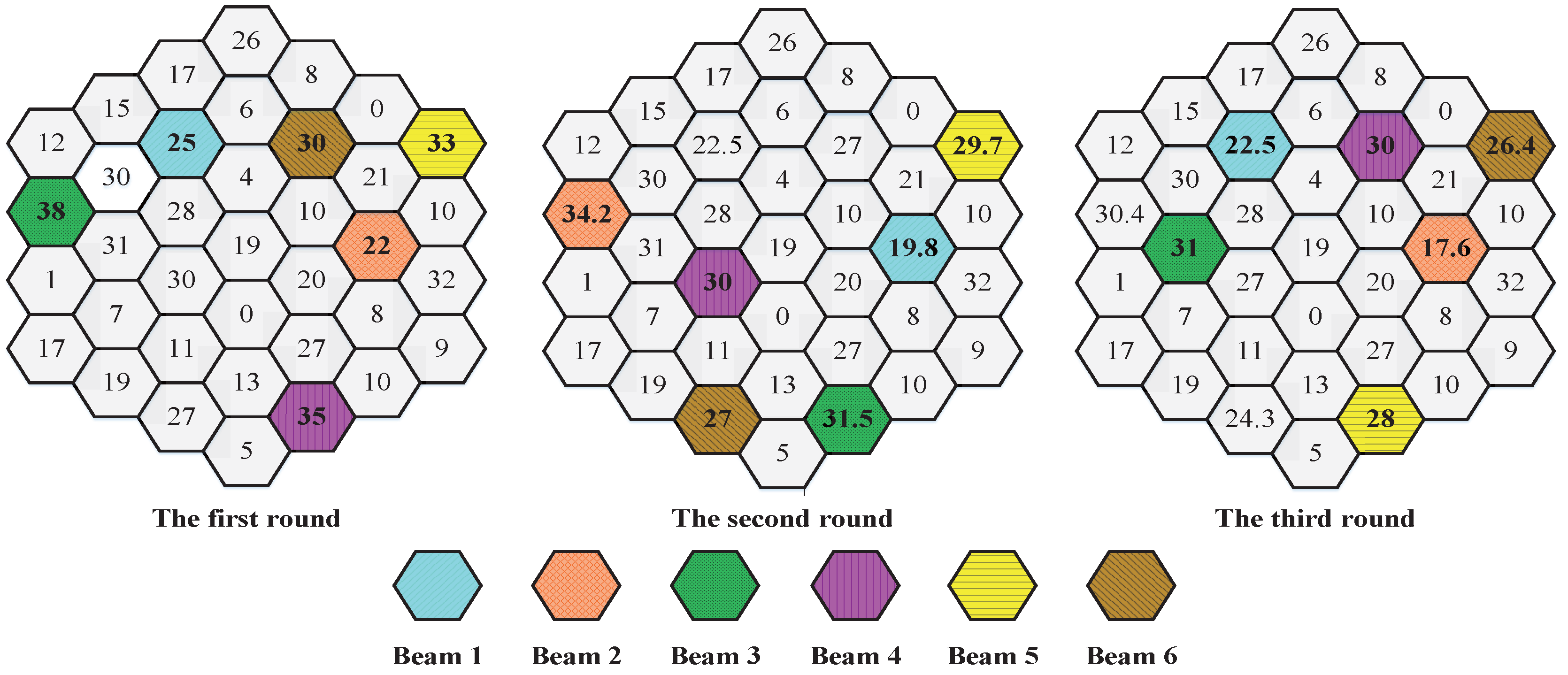
Upon receiving all input conditions, the beam-hopping pattern can be calculated via Algorithm 1. Figure 2 illustrates the results of the first three rounds of beam-hopping scheduling. Each beam (Beam 1 to Beam 6) is represented by a distinct pattern for clear identification. Assuming 20 beam-hopping time slots within each scheduling cycle, the six beams collectively occupy 120 time slots in total.
In the first round of scheduling, Beams 1 and 2 are first deployed to serve cells 11 and 31, respectively, which are assigned with high priority and carry time-sensitive traffic. The remaining cells are then scheduled by adopting a heuristic scheduling algorithm. Starting from cell 2, which yields the maximum weighted gain, Beams 3, 4, 5, and 6 are sequentially assigned to serve cells 2, 26, 34, and 23, while taking into account factors such as inter-beam co-channel interference and fairness.
After updating the weighted gains of all cells, the second round of scheduling is initiated. Since cell 11 can be re-served after an interval of one time slot, Beam 1 is preferentially allocated to serve cell 31. The remaining cells are served by Beams 2 to 6 based on their updated weighted gains.
Subsequently, the third round of scheduling commences. As both cells 11 and 31 require priority service in this round, Beam 1 is first dispatched to serve cell 11, followed by Beam 2 for cell 31, according to their respective weighted gains. The remaining cells are then covered by Beams 3 to 6 using the aforementioned heuristic algorithm.
Figure 2.
Example of beam-hopping scheduling.
In view of the practical application scenarios of the beam-hopping system for LEO constellations, this paper adopts the aforementioned beam-hopping scheduling scheme oriented to high-priority and time-sensitive services. On this basis, beams are scheduled preferentially to guarantee the transmission requirements of high-priority and time-sensitive services. Meanwhile, by conducting benefit-cost accounting, the system gain of the beam-hopping system is formally defined. Furthermore, a novel beam-hopping scheduling algorithm based on system gain is proposed in LEO satellite networks. The proposed method enables beam scheduling that better conforms to actual engineering operation conditions.
With the experimental scenario and parameter settings depicted in Figure 1, simulation experiments are carried out to analyze the system gain and user satisfaction, with a particular focus on the QoS guarantee performance of high-priority and time-sensitive services. It should be noted that the same hard constraint applied to the HBSA is also imposed on the round-robin and MWC schemes, ensuring a fair basis for performance comparison.
Figure 3 depicts the system gain versus the total service demand for the seven considered scheduling schemes. As the service demand increases from 200 to 2000 units, all algorithms exhibit a monotonic increase in system gain, yet with markedly different growth rates and saturation levels. The proposed HBSA consistently outperforms the Round-Robin, EDF, ACO, and GA schemes across the entire demand range. Notably, HBSA achieves a system gain of at low demand (200 units), which is approximately twice that of Round-Robin () and EDF (), and it maintains a stable lead of about over these baseline schemes as demand grows. When compared with the near-optimal MWC algorithm, HBSA achieves comparable performance at moderate to high loads (e.g., vs. at 1200, and vs. at 2000), while incurring significantly lower computational complexity. The GRL-BHS scheme, leveraging graph reinforcement learning, provides the highest system gain across all load levels (from at 200 to at 2000), slightly surpassing both MWC and HBSA. However, the performance gap between GRL-BHS and HBSA remains within for most load conditions, confirming that HBSA achieves near-optimal gain with much lower implementation overhead. These results validate the effectiveness of the proposed HBSA in delivering high system gain while maintaining practical feasibility for LEO satellite networks.
Figure 3.
Simulaiton result of system gain vs. service requirements.
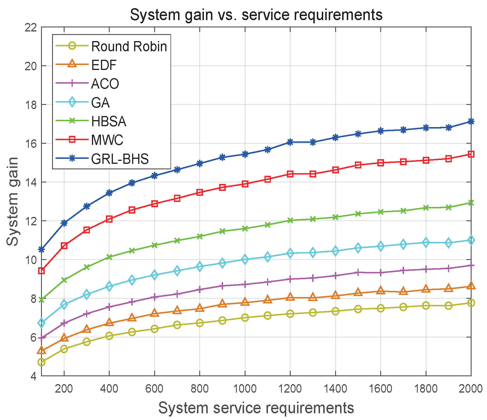
Figure 4 illustrates the user satisfaction level across 37 cells for the seven considered scheduling schemes. As shown in the table, the vast majority of cells achieve satisfaction under all algorithms, indicating that each scheme is capable of meeting user demands in most cells under the given simulation settings. However, notable exceptions are observed in Cell 1, where the Round-Robin scheme yields a satisfaction of only , while all other algorithms (EDF, ACO, GA, HBSA, MWC, and GRL-BHS) achieve between and . This significant discrepancy suggests that Round-Robin, lacking any priority or load-awareness mechanism, fails to allocate sufficient resources to this particular cell, which presumably has a disproportionately high traffic demand or unfavourable channel conditions. In contrast, the proposed HBSA achieves satisfaction in Cell 1, comparable to MWC and GRL-BHS, confirming its ability to adapt to non-uniform traffic distributions. Another interesting observation is Cell 29, where GA attains satisfaction, which may indicate an overservice scenario where the algorithm allocates more resources than strictly required, reflecting the less efficient resource utilisation of evolutionary approaches. Overall, Figure 4 demonstrates that HBSA consistently delivers satisfaction levels on par with the near-optimal MWC and GRL-BHS schemes across all cells, while substantially outperforming Round-Robin in challenging cells, thereby validating its effectiveness in ensuring user-level quality of service.
Figure 5 depicts the system overhead versus the total service demand for the seven considered scheduling schemes. The overhead values are presented on a logarithmic scale, with all algorithms exhibiting a general increasing trend as the demand grows from 200 to 2000 units. However, the growth rates differ considerably among the schemes. The proposed HBSA consistently maintains the lowest overhead across the entire demand range, with values around across all load levels, demonstrating its stable and efficient resource utilisation. In contrast, the MWC algorithm, while achieving near-optimal system gain, incurs substantially higher overhead, with its overhead increasing from at low demand to over at high demand (as indicated by the parenthetical values), reflecting the exponential complexity of its clique-search-based optimisation. The Round-Robin and EDF schemes maintain relatively constant overhead, yet their overhead levels are consistently higher than that of HBSA, due to inefficient beam utilisation and increased signalling interactions. The GRL-BHS scheme, leveraging graph reinforcement learning, achieves performance comparable to HBSA in terms of overhead (around for most load conditions), confirming its practical feasibility for onboard deployment, provided that the inference engine is appropriately optimised. Overall, Figure 5 demonstrates that HBSA strikes the most favourable balance between system performance and operational overhead, particularly under heavy-load conditions, where its overhead growth rate is significantly slower than that of MWC and other benchmark algorithms, thereby confirming its practical deployability in resource-constrained LEO satellite platforms.
In addition, the proposed scheme achieves a favorable balance of time slot allocation between low-gain and high-gain regions, thereby generating greater system benefits. Furthermore, it boosts the overall system gain and enhances the satisfaction of high-priority and time-sensitive users. Meanwhile, the system overhead is reduced, and an optimal comprehensive performance balance of the entire system is realized.
To quantify the fairness of resource allocation among cells for different algorithms, we adopt the Jain’s fairness index, defined as,
where denotes the number of time slots allocated to cell k during the scheduling period. The index ranges from to 1, with a value closer to unity indicating a more equitable distribution of resources.
Figure 5.
Simulaiton result of system overheads vs. service requirements.
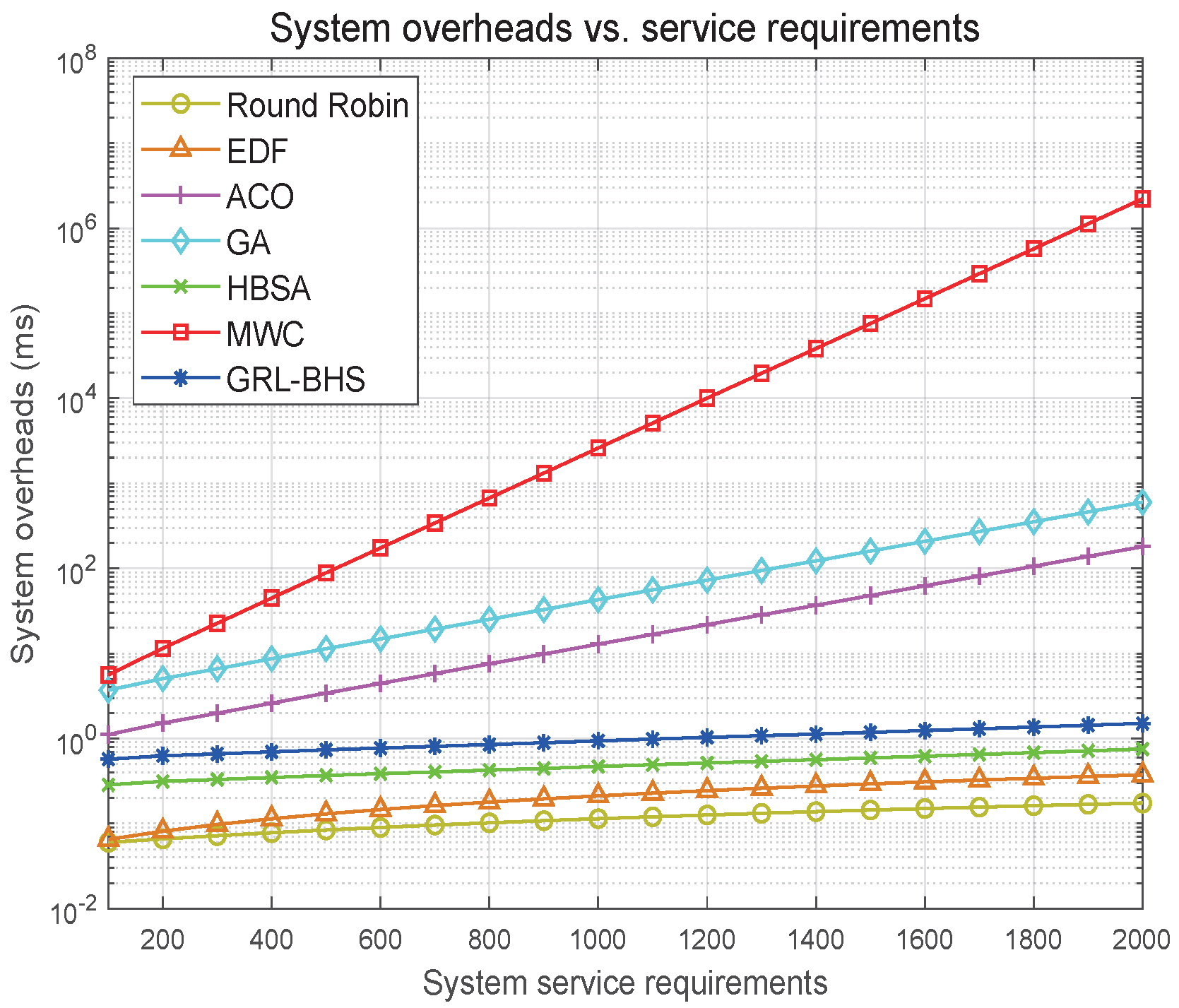
Figure 6 presents the Jain fairness index versus the normalized traffic load for the seven considered scheduling schemes. As the traffic load increases from to , all algorithms exhibit a declining trend in fairness, yet with considerably different rates of decrease. The Round-Robin scheme maintains an almost perfect fairness index of approximately across all load levels, as it allocates resources in a strictly round-robin manner regardless of traffic variations. The EDF scheme follows closely, with a gradual decline from to , reflecting its deadline-aware prioritisation which still preserves reasonable fairness. The proposed HBSA achieves a fair index of at low load, decreasing to at high load, which represents a well-balanced trade-off between system gain and fairness. The GRL-BHS scheme exhibits a slightly lower fairness index than HBSA, ranging from to , because its reinforcement learning policy tends to favour high-gain cells more aggressively in pursuit of higher system gain. The GA and ACO schemes show moderate fairness degradation, from and down to and , respectively, due to their inherent stochastic search biases. The MWC algorithm, which exclusively maximises total weighted gain, yields the lowest fairness across all load levels (from to ), confirming that its greedy preference for high-weight cells inevitably sacrifices equity among cells. Overall, Figure 6 demonstrates that HBSA strikes a favourable balance between fairness and system gain, achieving competitive fairness comparable to GRL-BHS and GA, while substantially outperforming MWC, thereby validating its effectiveness in ensuring equitable resource allocation across cells with non-uniform traffic demands.
8. Conclusion and Future Works
8.1. Conclusion
This paper has addressed the beam hopping scheduling problem in LEO satellite networks with a focus on high-priority and time-sensitive services by establishing a system gain maximization model and proposing a heuristic beam scheduling algorithm (HBSA) that pre-schedules time-critical traffic and greedily allocates remaining resources under interference and fairness constraints, achieving a desirable trade-off between performance and complexity. Extensive simulations, benchmarked against Round-Robin, EDF, ACO, GA, MWC, and an extended graph-reinforcement-learning scheme (GRL-BHS), demonstrate that HBSA delivers near-optimal system gain (comparable to MWC and GRL-BHS with a gap of less than under most load conditions), ensures satisfaction for high-priority services, maintains a Jain fairness index above even under heavy load, and reduces signalling overhead by an order of magnitude compared to online learning approaches, all while preserving a low polynomial complexity of that is practically deployable on resource-constrained LEO platforms. While the GRL-BHS extension offers the highest gain at the cost of offline training and moderate overhead, HBSA stands out as the most balanced and immediately viable solution for real-world LEO satellite systems, providing a solid foundation for future intelligent and adaptive beam-hopping scheduling in mega-constellations.
8.2. Future Works
Although the proposed heuristic algorithm shows promising performance, several aspects can be further explored to enhance the beam-hopping scheduling in LEO mega-constellations.
Adaptive Beam-Hopping Pattern Design:The current model assumes a fixed number of beams and time slots. Future research can extend it to an adaptive framework that dynamically adjusts the beam-hopping pattern according to real-time traffic prediction and satellite mobility. This would enable the system to better match time-varying service demands and channel conditions, further improving resource utilization.
Deep Reinforcement Learning for Distributed Scheduling: The heuristic algorithm presented in this paper relies on centralized ground control. Future work can integrate deep reinforcement learning (DRL) techniques, allowing each satellite or even each beam to act as an agent that learns an optimal scheduling policy in a distributed manner. Such an approach would reduce signaling overhead, enhance scalability, and improve robustness against dynamic constellation topologies.
Coordination with Non-Orthogonal Multiple Access and Full-Duplex Communication: The synergy between beam-hopping and advanced transmission schemes, such as non-orthogonal multiple access (NOMA) and full-duplex communication, remains largely unexplored. Future studies can investigate joint optimization of beam-hopping patterns with NOMA clustering and power allocation, as well as full-duplex operation, to further boost spectral efficiency and reduce latency for high-priority services.
Impact of Inter-Satellite Links on Beam Hopping Scheduling: In mega-constellations, inter-satellite links (ISLs) enable data relaying among satellites and may significantly affect traffic flow and resource allocation. Future work should incorporate ISL constraints and opportunities into the beam hopping scheduling model, considering end-to-end delay, multi-hop routing, and load balancing across the whole network.
Experimental Validation Using Hardware-in-the-Loop or Real Satellite Testbeds: While simulation results demonstrate the effectiveness of the proposed method, practical fading, handover procedures, and signaling delays can affect real-world performance. Future efforts should focus on experimental validation using hardware-in-the-loop (HIL) platforms or actual satellite testbeds, thereby assessing the algorithm’s feasibility and robustness under realistic operational conditions.
Author Contributions
Conceptualization, Liang Gou; Methodology, Liang Gou; Software, Yulei Nie and Wei Sun; Validation, Yulei Nie; Investigation, Liang Gou; Resources, Wei Sun and Gengxin Zhang; Data curation, Wei Sun and Ziwei Liu; Writing – review & editing, Ziwei Liu; Visualization, Dapeng Qi; Supervision, Dapeng Qi; Funding acquisition, Gengxin Zhang. All authors have read and agreed to the published version of the manuscript.
Funding
This work was supported by the National Natural Science Foundation of China (NSFC) under Grant U21A20450.
Institutional Review Board Statement
Not applicable.
Informed Consent Statement
Not applicable.
Data Availability Statement
The original contributions presented in this study are included in the article. Further inquiries can be directed to the corresponding author.
Conflicts of Interest
The authors declare no conflicts of interest.
References
- Feng, Y. Z.; Sun, Y. H.; Peng, M. G. Performance Analysis in Satellite Communication With Beam Hopping Using Discrete-Time Queueing Theory. IEEE Internet Things J. 2024, vol. 11(no. 7), 11679–11692. [Google Scholar] [CrossRef]
- Sun, H.; Jing, W. P.; Lu, Z. M.; Wen, X. M.; Li, W. An Energy-Efficient Beam Hopping Strategy in Interference Coexistence Satellite Systems. Proc. 2024 - IEEE/CIC International Conference on Communications in China (ICCC Workshops), Hangzhou, China, 2024; pp. 711–716. [Google Scholar]
- Lin, Z. Y.; Ni, Z. Y.; Kuang, L. L.; Jiang, C. X.; Huang, Z. Multi-Satellite Beam Hopping Based on Load Balancing and Interference Avoidance for NGSO Satellite Communication Systems. IEEE Trans. Commun. 2023, vol. 71(no. 1), 282–295. [Google Scholar] [CrossRef]
- Liu, Zijun; Wang, Yafei; Wang, Wenjin; Sun, Yi; Yan, Hong; Sun, Zhili. Multi-Satellite Coordinated Beam Hopping for Interference Mitigation Under Tilted Beam Effects: A Graph-Theoretic Approach. IEEE Wirel. Commun. Lett. 2026, vol. 15, 2313–2317. [Google Scholar] [CrossRef]
- Deng, H. M.; Ying, K.; Feng, D. Q.; Gui, L.; He, Y. Z.; Xia, X. G. Satellites Beam Hopping Scheduling for Interference Avoidance. IEEE J. Sel. Areas Commun. 2024, vol. 42(no. 12), 3647–3658. [Google Scholar] [CrossRef]
- Shi, T.; Liu, Y. Y.; Kang, S. L.; Sun, S. H.; Liu, R. K. Angle-Based Multicast User Selection and Precoding for Beam-Hopping Satellite Systems. IEEE Trans. Broadcast. 2023, vol. 69(no. 4), 856–871. [Google Scholar] [CrossRef]
- Han, Z. H.; Yang, T.; Liu, R. K.; Jiao, S. Beam Hopping Pattern Design using Viterbi Algorithm for Satellite Communication Systems. Proc. 2023 - IEEE International Conference on Communications (ICC2023), Hangzhou, China, 2024; pp. 711–716. [Google Scholar]
- Ha, V. N.; Nguyen, T. T.; Lagunas, E.; Duncan, J. C. M.; Chatzinotas, S. GEO Payload Power Minimization: Joint Precoding and Beam Hopping Design. Proc. 2022 IEEE Global Communications Conference, Rio de Janeiro, Brazil, 2023; pp. 6445–6450. [Google Scholar]
- Han, Z. H.; Yang, T.; Liu, R. K. On Beam Hopping Pattern Design for Satellite Communication Systems With Hybrid Precoding. IEEE Trans. Veh. Technol. 2024, vol. 73(no. 1), 1364–1369. [Google Scholar] [CrossRef]
- Chen, L.; Ha, V. N.; Lagunas, E.; Wu, L. L.; Chatzinotas, S.; Ottersten, B. The Next Generation of Beam Hopping Satellite Systems: Dynamic Beam Illumination With Selective Precoding. IEEE Trans. Wirel. Commun. 2023, vol. 22(no. 4), 2666–2682. [Google Scholar] [CrossRef]
- Liu, H. Y.; Zhang, R. H.; Jing, X. J. Beam Hopping for Multi-Beam LEO Satellite Systems with Integrated Sensing and Communications. Proc. 2024 - IEEE Wireless Communications and Networking Conference (WCNC2024), Dubai, United Arab Emirates, 2024; pp. 1–6. [Google Scholar]
- Lyu, L. Y.; Qi, C. H. Beam Position and Beam Hopping Design for LEO Satellite Communications. China Commun. 2023, vol. 20(no. 7), 29–42. [Google Scholar] [CrossRef]
- Jia, H. Q.; Wang, Y.; Peng, H. X.; Li, W. Dynamic Beam Hopping and Resource Allocation for Non-Uniform Traffic Demand in NGSO Satellite Communication Systems. IEEE Trans. Veh. Technol. 2025, vol. 74(no. 1), 816–830. [Google Scholar] [CrossRef]
- Zhang, X.; Zhao, L.; Gao, P. Z.; Li, J. W. Energy Efficient Downlink Resource Allocation in Beam Hopping LEO Satellite Communication Systems. Proc. 2024 IEEE/CIC International Conference on Communications in China (ICCC Workshops), Hangzhou, China, 2024; pp. 675–680. [Google Scholar]
- Zheng, S.; Zhang, X.; Wang, P.; Wang, W. B. Joint Beam Scheduling and Power Optimization for Beam Hopping LEO Satellite Systems. China Commun. 2024, vol. 21(no. 10), 1–14. [Google Scholar] [CrossRef]
- S. M. Zamacola, N. P.; Rodríguez-Osorio, R. M.; Cameron, B. G. Joint Illumination, Power, and Band Allocation for Multi-Beam LEO Satellites With Beam-Hopping Using Mixed-Integer Linear Programming. IEEE Trans. Wirel. Commun. 2026, vol. 25, 15710–15724. [Google Scholar] [CrossRef]
- Zhao, X. Y.; Wang, C.; Cai, S. S.; Chen, R. Q.; Wen, J. R.; Xu, L. X. Multi-Satellite Cooperative Load-Balancing Scheme Based on Dynamic Beam Coverage for LEO Beam Hopping Systems. IEEE Wirel. Commun. Lett. 2024, vol. 13(no. 10), 2892–2896. [Google Scholar] [CrossRef]
- Zheng, F.; Pi, Z.; Zhou, Z.; Ye, M.; Qiu, H. B. NOMA-based collaborative beam hopping frequency allocation mechanism for future LEO satellite systems. China Commun. 2023, vol. 20(no. 6), 321–338. [Google Scholar] [CrossRef]
- Li, T.; Yao, R. G.; Fan, Y.; Zuo, X. Y.; Miridakis, N. I.; Tsiftsis, T. A. Pattern Design and Power Management for Cognitive LEO Beaming Hopping Satellite-Terrestrial Networks. IEEE Trans. Cogn. Commun. Netw. 2023, vol. 9(no. 6), 1531–1545. [Google Scholar] [CrossRef]
- Lin, Z. Y.; Ni, Z. Y.; Kuang, L. L.; Jiang, C. X.; Huang, Zhen. Dynamic Beam Pattern and Bandwidth Allocation Based on Multi-Agent Deep Reinforcement Learning for Beam Hopping Satellite Systems. IEEE Trans. Veh. Technol. 2022, vol. 71(no. 4), 3917–3930. [Google Scholar] [CrossRef]
- Zheng, S.; Zhang, X.; Zhang, J. X.; Wang, P.; Wang, W. B. Traffic-Aware Resource Management of Beam Hopping in Satellite-Enabled Internet of Things. IEEE Internet Things J. 2024, vol. 11(no. 21), 34504–34518. [Google Scholar] [CrossRef]
- Meng, M.; Hu, B.; Chen, S. Z.; Kang, S. L. Dynamic Beam Pattern Based on Cooperation Multi-Agent VDN-D3QN for LEO Satellite Communication System. IEEE Trans. Green Commun. Netw. 2025, vol. 9(no. 2), 725–738. [Google Scholar] [CrossRef]
- Xu, G. L.; Tan, F.; Ran, Y. Y.; Zhao, Y. Y.; Luo, J. T. Joint Beam-Hopping Scheduling and Coverage Control in Multibeam Satellite Systems. IEEE Wirel. Commun. Lett. 2022, vol. 12(no. 2), 267–271. [Google Scholar] [CrossRef]
- Lin, Z. Y.; Ni, Z. Y.; Kuang, L. L.; Jiang, C. X.; Huang, Z. Satellite-Terrestrial Coordinated Multi-Satellite Beam Hopping Scheduling Based on Multi-Agent Deep Reinforcement Learning. IEEE Trans. Wirel. Commun. 2024, vol. 23(no. 8), 10091–10103. [Google Scholar] [CrossRef]
- Ran, Y. Y.; Tan, F.; Chen, S. W.; Lei, J. Z.; Luo, J. T. Towards Beam Hopping and Power Allocation in Multi-Beam Satellite Systems With Parameterized Reinforcement Learning. IEEE Trans. Veh. Technol. 2024, vol. 73(no. 9), 14050–14055. [Google Scholar] [CrossRef]
- Liu, H. T.; Wang, Y. C.; Wang, T.; Li, P. X. User-Level Dynamic Beam Hopping Design for LEO Satellite Networks Based on Deep Reinforcement Learning Assisted Enhanced Genetic Algorithm. Proc. 2024 IEEE 99th Vehicular Technology Conference (VTC2024-Spring), Singapore, Singapore, 2024; pp. 1–7. [Google Scholar]
- Tesfaw, B. A.; Juang, R. T. Multiagent DRL-Based Dynamic Beam Hopping and Resource Allocation in LEO Satellite Communication Systems. IEEE Trans. Aerosp. Electron. Syst. 2026, vol. 62, 9908–9923. [Google Scholar] [CrossRef]
- Wen, R. Q.; Jin, J.; Lin, Z. Y.; Kuang, L. L. Attention-Based Cooperative Beam Hopping Scheduling via Multi-Agent Communication in NGSO Satellite Networks. IEEE Trans. Wirel. Commun. 2026, vol. 25, 17709–17723. [Google Scholar] [CrossRef]
- Wang, J.; Qi, C. H.; Yu, Shui. Hybrid Beamforming Design for Beam-Hopping LEO Satellite Communications. Proc. 2023 IEEE Global Communications Conference (GLOBECOM 2023), Kuala Lumpur, Malaysia, 2023; pp. 3959–3964. [Google Scholar]
- Wang, J.; Qi, C. H.; Yu, S.; Mao, S. W. Joint Beamforming and Illumination Pattern Design for Beam-Hopping LEO Satellite Communications. IEEE Trans. Wirel. Commun. 2024, vol. 23(no. 12), 18940–18950. [Google Scholar] [CrossRef]
- Li, Z. Q.; Wang, S. J.; Han, S.; Meng, W. X.; Li, C. Joint Design of Beam Hopping and Multiple Access Based on Cognitive Radio for Integrated Satellite-Terrestrial Network. IEEE Netw. 2023, vol. 37(no. 1), 36–43. [Google Scholar] [CrossRef]
Figure 1.
Configuration and initial service traffic of cells. (a) Configuration of cells. (b) Initial service traffic of cells.
Figure 1.
Configuration and initial service traffic of cells. (a) Configuration of cells. (b) Initial service traffic of cells.
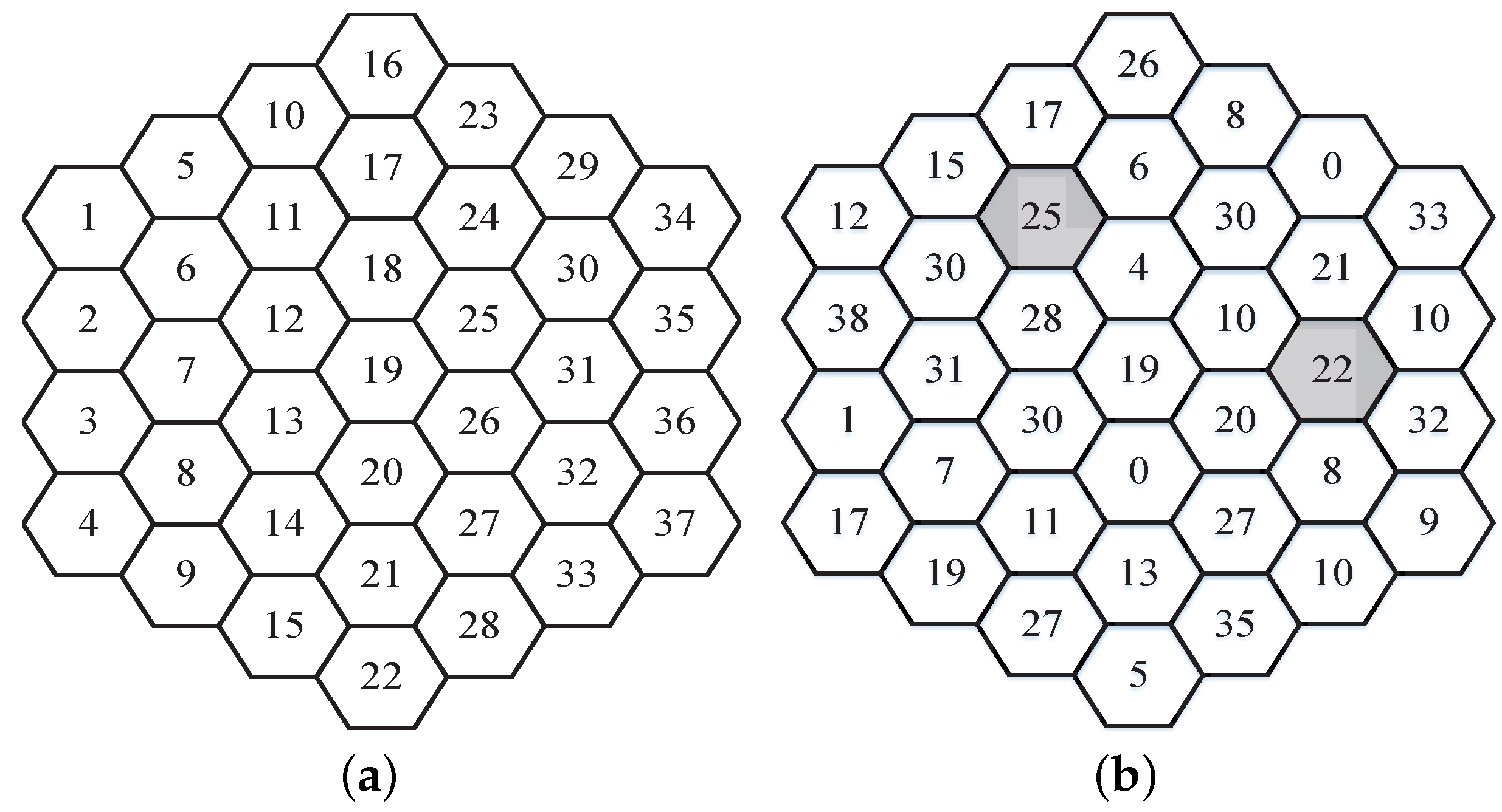
Figure 4.
Simulaiton result of user satisfaction vs. cell number.
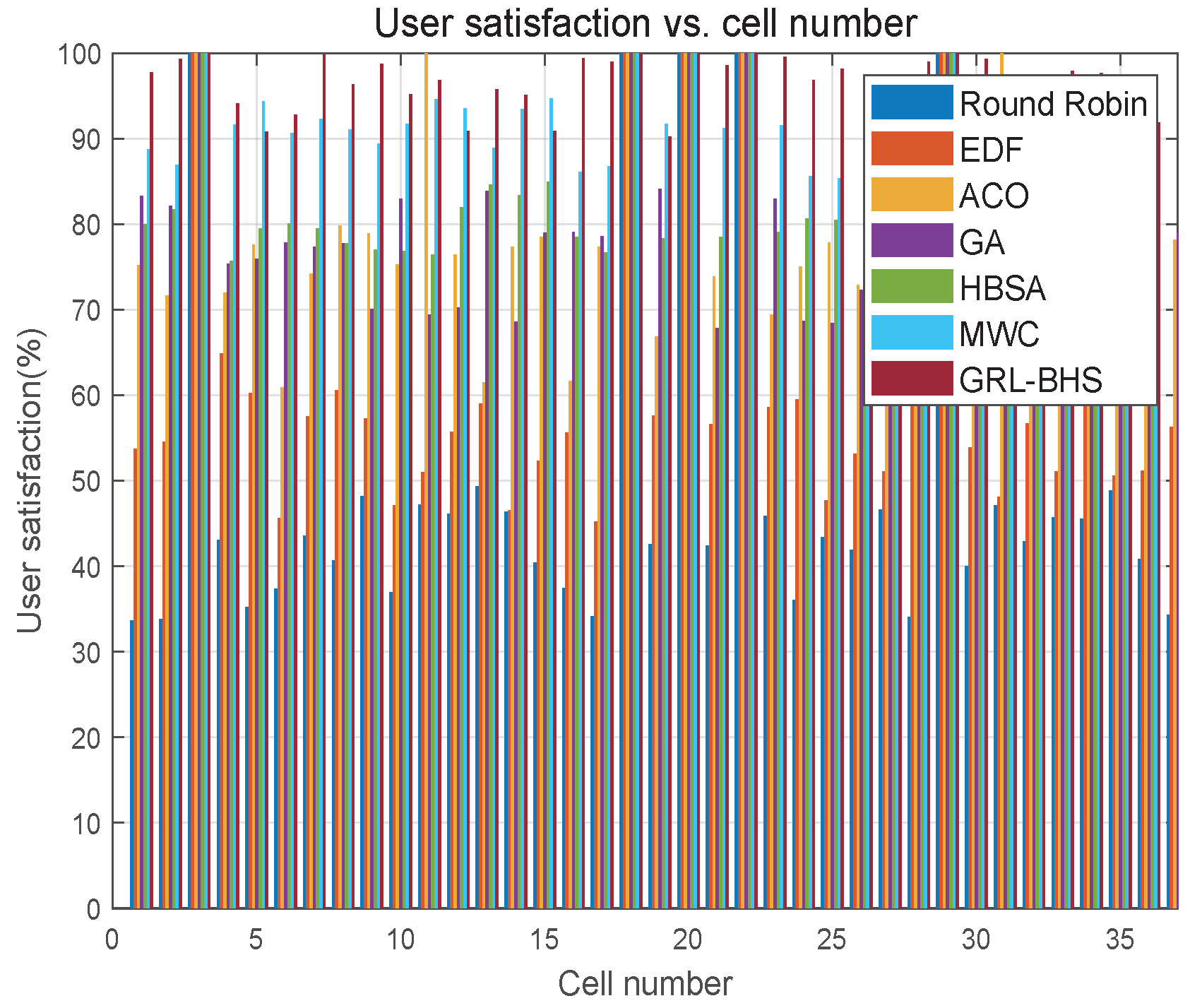
Figure 6.
Simulaiton result of Jain’s fairness index vs. normalized traffic load.
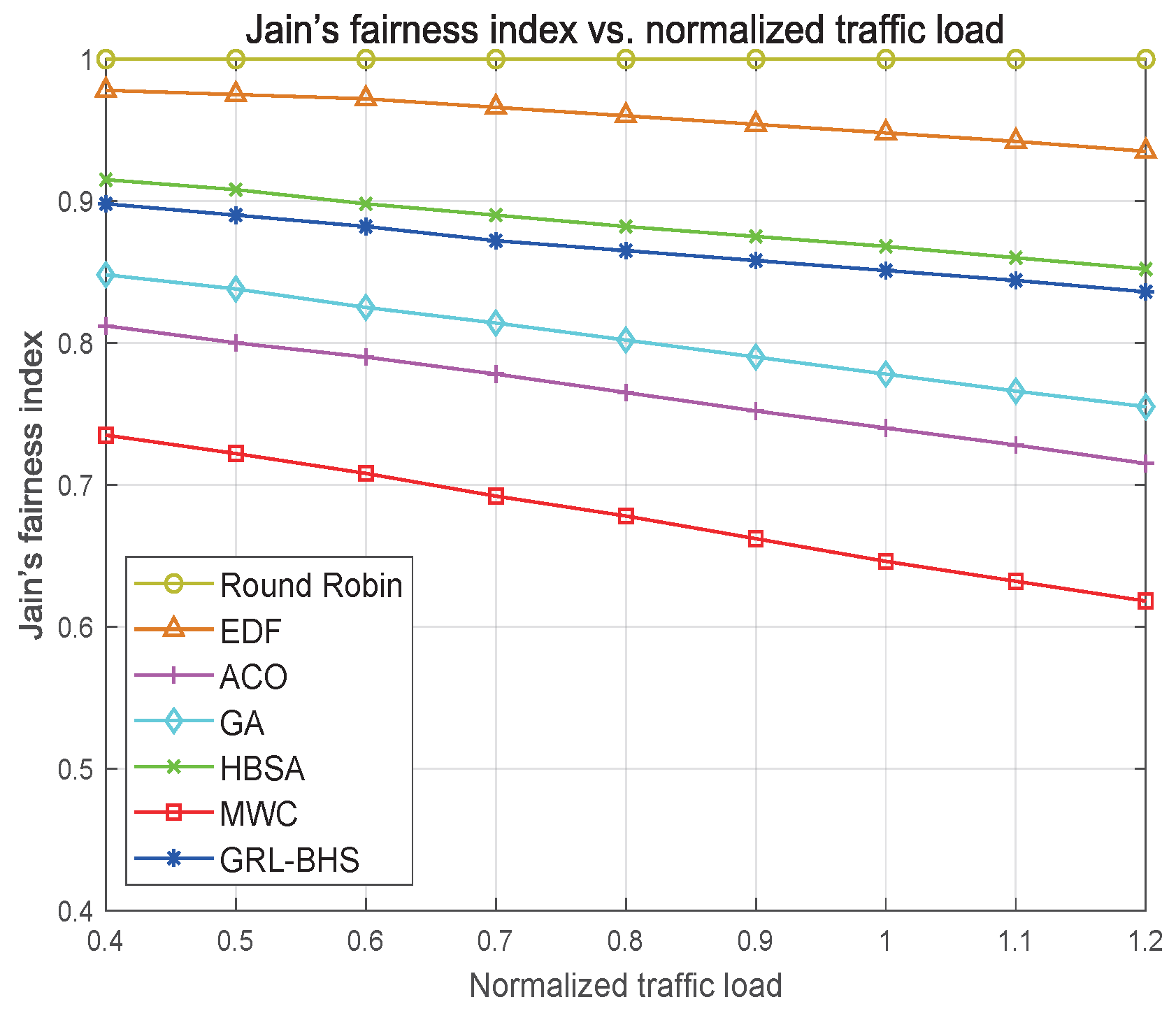
Disclaimer/Publisher’s Note: The statements, opinions and data contained in all publications are solely those of the individual author(s) and contributor(s) and not of MDPI and/or the editor(s). MDPI and/or the editor(s) disclaim responsibility for any injury to people or property resulting from any ideas, methods, instructions or products referred to in the content. |
© 2026 by the authors. Licensee MDPI, Basel, Switzerland. This article is an open access article distributed under the terms and conditions of the Creative Commons Attribution (CC BY) license (http://creativecommons.org/licenses/by/4.0/).
Copyright: This open access article is published under a Creative Commons CC BY 4.0 license, which permit the free download, distribution, and reuse, provided that the author and preprint are cited in any reuse.