Relational Observability of Semantic Timing: What Pooling Erases and Temporal Compression Preserves

1. Introduction: The Object Lost in the Average

Language research routinely pools the observers whose timing generated the effect. In the present data, pooling preserved the familiar semantic-negativity response and eliminated the observer-level timing–localization relation. These outcomes are not contradictory. They are different estimands.

1.1. The Group Effect and the Observer Relation

A group-average ERP asks whether a semantic effect exists and where it appears on average. It combines participant-level signals into a population profile and identifies the temporal region in which an experimental contrast is expressed most clearly. For semantic processing, this approach has made the N400 one of the most stable and recognizable effects in cognitive neuroscience [13,14].

An observer-paired relation asks a different question. It asks whether independently estimated properties of the response recur together across individuals. In the present study, those properties are timing and temporal localization. The empirical object is the across-observer relation between when a participant’s semantic-negativity profile peaks and where that participant’s response is concentrated across the analysis window.

The population effect and the observer relation are not interchangeable. A stable average waveform does not determine whether participants who peak later also express later temporal localization. Likewise, a structured observer relation does not require the group-average waveform to vary across participants in an obvious or visually dramatic way. The two objects occupy different statistical coordinates [6,17].

This distinction is central to individual-differences research. Tasks that produce stable population effects do not automatically provide reliable measures of between-person variation, because the conditions that stabilize a mean can reduce or obscure the variance required for correlational inference [10]. Observer-level claims therefore require a psychometric treatment of participant effects rather than an assumption that a replicable experimental contrast is automatically suitable for individual-differences analysis [19].

The relation studied here requires observer identity as a coordinate. Each participant contributes a timing estimate and a localization estimate. The relation exists across the correctly paired set of those estimates. Once observer identity is removed, the relation is not weakened or blurred. Its defining coordinate no longer exists.

1.2. Pooling Transforms the Estimand

Pooling preserves the mean waveform because averaging retains the signal components shared across participants. When a semantic-negativity effect is broadly aligned in polarity and temporal region, the pooled profile can remain canonical even if participants differ in the exact timing and allocation of that effect.

Pooling also removes the participant axis. The resulting waveform contains one value at each time point rather than a set of observer-indexed timing and localization estimates. Between-observer covariance cannot be reconstructed after the observers have been collapsed.

This is loss of the estimand, not merely loss of precision.

For population contrasts, averaging can improve the visibility and stability of a shared effect. For an observer-paired relation, the same operation removes the coordinate on which the relation is defined. The order of operations therefore matters: construct the observer-level quantities and their relation while observer correspondence remains intact, then aggregate the evidence. Aggregating observers first changes the scientific object.

1.3. Disjoint Reconstruction as the Decisive Test

A second problem arises if timing and localization are extracted from the same waveform. Measures derived from the same samples can correlate because they share noise, shape, amplitude, or algebraic structure. A later peak may mechanically shift a localization estimate even when no stable observer organization exists beyond that waveform.

The decisive test is therefore reconstruction across disjoint observations.

For each participant, eligible trials are divided into disjoint condition-stratified halves. One half supplies the timing estimate. The other supplies the temporal-localization estimate. The analysis is then reversed: localization is estimated from the first half and timing from the second. The two directional relations are transformed to Fisher z, averaged, and returned to correlation scale as a symmetric cross-fit estimate.

This procedure separates the samples used to estimate the two quantities. Any recurring relation must cross the trial split. It cannot be generated solely by shared trial noise within one waveform.

Observer identity then becomes the reconstruction key. The timing estimate from one half is paired with the localization estimate from the other half for the same participant. The shared observer-pairing null breaks that correspondence by applying the same reassignment of observer labels across the dependent directional analyses. The null preserves the marginal timing and localization values while destroying the participant-level mapping between them.

This design distinguishes a waveform identity from a recurring observer relation. A same-waveform correlation may reflect the geometry of one profile. A cross-fit observer-paired correlation requires the relation to survive sample separation and correct identity matching.

Repeated trial allocations extend the same logic. They test whether the relation recurs across many admissible partitions rather than depending on one convenient split. These allocations are dependent stability checks, not independent replications, but they reveal whether the primary result is tied to a fragile assignment of trials.

1.4. Contributions

This paper tests and revises ODER through three contributions. First, it reconstructs the observer-paired timing organization predicted by ODER across disjoint neural and behavioral observations and shows that recovery depends on correct observer correspondence. Second, it identifies a transformation profile: pooling, reassignment, desynchronization, and gradient erasure remove coordinates required by the tested relations, while severe temporal compression and removal of ERP rectification preserve recovery; signed temporal allocation reveals the strongest behavioral organization. Third, it establishes relational observability as a measurement principle and supplies a pre-analysis test of whether a retained dataset preserves the observer-indexed measurement object required by the claim. A transformation can discard many values while preserving a scientific relation, or retain a detailed signal while eliminating the relation’s defining coordinate.

A population effect, an individual timing estimate, and a relation among independently estimated observer measures are different scientific objects. Language-processing pipelines must preserve the coordinates required by the object they intend to measure.

2. The ODER Prediction and Relational Observability

ODER treats semantic access as observer-indexed temporal organization. The empirical test is whether timing and localization estimated from separate observations can be reunited through correct observer identity.

2.1. Access Under Observer Constraints

Observer-Dependent Entropy Retrieval begins from a simple claim about access. Linguistic structure does not become available to every observer at the same moment or through the same temporal organization. Access unfolds over observer-indexed time, under finite attention, memory, familiarity, interference, and measurement constraints.

This makes timing part of the phenomenon.

On a temporally resolved neural surface, observer-specific access organization must appear through temporal form. Onset, width, asymmetry, gradient, peak placement, and early–late distribution are therefore not automatically external confounds. They are candidate observable expressions of how access unfolds. The empirical problem is to distinguish stable temporal organization that recurs through the observer from algebraic coupling, response magnitude, sample-specific noise, and other properties that do not survive disjoint estimation or correct-pairing tests. Variation in latency or temporal allocation cannot be classified as residual noise before testing whether it carries stable observer structure. Some variation will reflect measurement error, waveform morphology, exposure, or general processing speed. The theory predicts that another component may arise from how access unfolds for a particular observer.

This observer-indexed prediction follows the bounded-access formulation of ODER [3]. The empirical question is therefore narrower than a complete theory of comprehension. It does not ask whether one timing measure directly reveals retrieval, or whether a single neural or behavioral surface identifies the mechanism that produced it. It asks whether temporal properties recur in an observer-indexed way across independently observed data.

Under this prediction, an observer who expresses a later timing estimate should also tend to express a later temporal localization or allocation estimate, even when those quantities are constructed from separate observations. The relevant structure is relational. Neither timing nor localization alone is the primary object. The object is their recurrence through observer identity.

This prediction can be tested on different measurement surfaces. In ERP data, timing and localization are properties of a participant-specific semantic-negativity profile. In self-paced reading, timing and allocation are expressed through the distribution of reading-time structure across current and downstream positions. The operators differ across modalities, but the test remains the same: does temporal organization recur when independently estimated quantities are reunited through the correct observer?

2.2. The Observer-Paired Empirical Object

Let i index observers. For each observer, define a timing estimate

$$T_i,$$

and a temporal localization or allocation estimate

$$L_i.$$

The observer-paired relation is

$$R(T,L)=corr\left({\left\{T_i\right\}}_{i=1}^N,{\left\{L_i\right\}}_{i=1}^N\right).$$

The relation is calculated across observers, but its components are constructed within observers. Each $T_i$ belongs to a particular participant or reader, and each $L_i$ belongs to that same participant or reader. Observer identity supplies the mapping between the two sets of estimates.

For observer-defined relations of the present kind, observer identity functions as more than a grouping label. It supplies the correspondence rule that makes timing and localization estimates constructed from disjoint observations belong to the same scientific unit. Removing that coordinate does not simply weaken their association. It removes the pairing required to define it.

In the ERP analysis, the two quantities are built from disjoint trial halves. Let

$$T_i^{\left(A\right)}$$

denote timing estimated from trial half A, and let

$$L_i^{\left(B\right)}$$

denote localization estimated from trial half B. One directional relation is

$$R_{A\to B}=corr\left({\left\{T_i^{\left(A\right)}\right\}}_{i=1}^N,{\left\{L_i^{\left(B\right)}\right\}}_{i=1}^N\right).$$

The reverse direction is

$$R_{B\to A}=corr\left({\left\{T_i^{\left(B\right)}\right\}}_{i=1}^N,{\left\{L_i^{\left(A\right)}\right\}}_{i=1}^N\right).$$

The two directional coefficients are transformed to Fisher z, averaged, and converted back to correlation scale. This yields the symmetric cross-fit estimate

$$R_{\mathrm{sym}}=tanh\left[{\displaystyle \frac{atanh\left(R_{A\to B}\right)+atanh\left(R_{B\to A}\right)}{2}}\right].$$

The same logic applies to the behavioral analyses, with disjoint story partitions replacing trial halves and reader-specific temporal operators replacing ERP operators.

Correct pairing reunites the estimates through observer identity. The timing value for observer i is paired with the localization value for observer i. Random reassignment breaks this correspondence. If $\pi$ is a permutation of observer labels, the reassigned relation is

$$R_{\pi }=corr\left({\left\{T_i\right\}}_{i=1}^N,{\left\{L_{\pi \left(i\right)}\right\}}_{i=1}^N\right).$$

The reassignment preserves the marginal timing and localization distributions. It changes only which observer’s timing is paired with which observer’s localization. A relation that depends on correct pairing should exceed the distribution generated by these reassigned mappings.

The empirical object is therefore neither a waveform feature nor a generic correlation among derived quantities. It is a relation that must survive sample separation and depend on correct observer correspondence.

2.3. Measurement Operators Preserve Different Coordinates

The experiments compare transformations that remove different properties of the measurement surface. Their effects cannot be understood through a single scale of information loss.

Table 1. Conceptual transformation map. Each operation changes a different coordinate of the measurement surface.

Transformation	Coordinate changed	Coordinate retained	Scientific test
Pooling	Observer identity	Group temporal profile	Whether the observer relation remains estimable after aggregation
Observer reassignment	Correct correspondence	Marginal timing and localization values	Whether recovery depends on the correct observer
Desynchronization	Temporal alignment	Observer identity and measured values	Whether the original temporal correspondence carries recovery
Gradient erasure	First-order temporal shape	Observer identity and residual variation	Whether temporal shape carries recovery on the tested surface
Temporal binning	Native cardinality and precision	Broad order and observer identity	Whether fine timing distinctions are required
Rectification removal	Nonnegative ERP geometry	Polarity orientation and operators	Whether the zero floor is required
Signed behavioral construction	Nonnegative concentration	Temporal direction and allocation	Whether signed lag structure carries reader organization

Table 1. Conceptual transformation map. Each operation changes a different coordinate of the measurement surface.

Transformation	Coordinate changed	Coordinate retained	Scientific test
Pooling	Observer identity	Group temporal profile	Whether the observer relation remains estimable after aggregation
Observer reassignment	Correct correspondence	Marginal timing and localization values	Whether recovery depends on the correct observer
Desynchronization	Temporal alignment	Observer identity and measured values	Whether the original temporal correspondence carries recovery
Gradient erasure	First-order temporal shape	Observer identity and residual variation	Whether temporal shape carries recovery on the tested surface
Temporal binning	Native cardinality and precision	Broad order and observer identity	Whether fine timing distinctions are required
Rectification removal	Nonnegative ERP geometry	Polarity orientation and operators	Whether the zero floor is required
Signed behavioral construction	Nonnegative concentration	Temporal direction and allocation	Whether signed lag structure carries reader organization

The behavioral surfaces require one additional distinction. The locked family represents lag structure as nonnegative concentration after clipping. The signed family uses operators designed for signed profiles and represents temporal allocation. They retain different coordinates and expose different relations.

2.4. Loss of Detail and Loss of Relation

Information loss is not one-dimensional. Pooling can retain the full sampled group waveform while removing observer identity. Three-bin compression can discard most native timing distinctions while preserving observer identity and broad temporal placement. The relevant question is which coordinates remain available for the relation being estimated. Smoothing, averaging, binning, normalization, rectification, clipping, and temporal warping therefore change the set of recoverable relations, not simply the amount of detail.

2.5. Predictions

The empirical program began with four predictions.

First, correct observer pairing should produce stronger recovery than observer reassignment. If timing and localization recur through stable observer organization, the correctly paired relation should exceed a null distribution that preserves the marginal estimates while breaking their correspondence.

Second, pooling should remove the observer relation while preserving the group-level effect. The pooled representation should retain the canonical semantic-negativity profile and the gross behavioral cost structure, but it should no longer support a relation defined across observers.

Third, auxiliary same-profile operator recovery should collapse under targeted temporal transformations. Desynchronization should disrupt the original temporal correspondence. Temporal-gradient erasure should remove the first-order temporal organization required to relate timing and localization on that tested surface. These transformations should weaken or eliminate same-profile operator recovery even when other properties of the signal remain.

Fourth, finer native timing was expected to support stronger recovery than severe temporal compression. The original prediction treated native temporal precision as part of the structure carrying the observer relation. Reducing timing to three broad categories was therefore expected to attenuate recovery.

The final prediction failed.

Three-bin timing preserved the relation. The result also persisted after zero rectification was removed. The failure of the native-resolution prediction changed the explanatory target. Fine timing precision was not the property that distinguished preservation from destruction. Observer identity, temporal alignment, broad order, sign, and allocation emerged as separate coordinates whose preservation had to be tested directly.

3. Experimental Progression and Analysis Status

The empirical program contains five inferential layers. Their status was fixed by when the analysis was declared and by the scientific question it answers.

Table 2. Experimental progression and inferential status. The complete analysis registry appears in Supplementary Appendix A.

Layer	Status	Scientific question	Primary evidence
ERP reconstruction	Locked primary	Do timing and localization recur across disjoint trial estimates through correct participant identity?	Symmetric cross-fit, observer bootstrap, pairing null
Natural Stories concentration	Locked primary	Do reader timing and nonnegative concentration recur across complementary story partitions?	Dependent family median, reader bootstrap, pairing null
ERP temporal compression	Prospectively frozen	Does severe reduction of timing cardinality weaken observer recovery?	Paired native-minus-three-bin contrast and resolution ladder
ERP and SPR operator sensitivities	Prospectively specified secondary	Are ERP recovery and behavioral organization carried by rectification or clipping?	Unrectified ERP, clipping audit, signed allocation family
Selected and post-diagnostic checks	Diagnostic	Does the concentration relation recur where clipping is inactive, and can tie handling explain the compression result?	Clipping-inactive subset and tie sensitivities

Table 2. Experimental progression and inferential status. The complete analysis registry appears in Supplementary Appendix A.

Layer	Status	Scientific question	Primary evidence
ERP reconstruction	Locked primary	Do timing and localization recur across disjoint trial estimates through correct participant identity?	Symmetric cross-fit, observer bootstrap, pairing null
Natural Stories concentration	Locked primary	Do reader timing and nonnegative concentration recur across complementary story partitions?	Dependent family median, reader bootstrap, pairing null
ERP temporal compression	Prospectively frozen	Does severe reduction of timing cardinality weaken observer recovery?	Paired native-minus-three-bin contrast and resolution ladder
ERP and SPR operator sensitivities	Prospectively specified secondary	Are ERP recovery and behavioral organization carried by rectification or clipping?	Unrectified ERP, clipping audit, signed allocation family
Selected and post-diagnostic checks	Diagnostic	Does the concentration relation recur where clipping is inactive, and can tie handling explain the compression result?	Clipping-inactive subset and tie sensitivities

The locked ERP analysis includes repeated trial allocations, pooling, observer reassignment, desynchronization, temporal-gradient erasure, and a descriptive amplitude-controlled estimate. Repeated allocations assess stability across admissible splits of the same data; they do not create independent replications. The amplitude-controlled estimate is descriptive because it was not assigned a separate interval or pairing test.

The locked Natural Stories family contains 1,250 dependent estimates across 125 scored partitions and ten eligible specifications. Its family median summarizes recurrence across a shared 96-reader measurement surface. The signed family answers a different operator question and retains secondary status. The clipping-inactive analysis uses smaller strata of 31 to 33 readers and retains selected-profile status.

The frozen compression test designated the native-versus-three-bin Fisher-z contrast before outcome inspection. Bin definitions, temporal boundaries, peak rules, tie handling, and shared resampling mappings were fixed with the prediction. The unrectified compression analysis repeated that structure as a prospectively specified secondary sensitivity.

Detailed operators, strata, seeds, resampling units, dependency structures, and artifact paths are reported in Methods and the supplementary registries. Analyses developed after inspection of the relevant outcome are labeled post-diagnostic and cannot alter the locked or frozen inference.

The sequence was adversarial by construction rather than an accumulation of favorable specifications. ODER would be weakened if the relation failed to cross disjoint estimates, if incorrect observer pairing performed similarly to correct pairing, if observer erasure or targeted disruption preserved the declared relation, or if recovery depended on rectification, clipping, or one convenient partition. The frozen compression experiment created an additional theoretical risk by testing the proposed role of native temporal precision. That prediction failed. The results therefore distinguish empirical support for observer-indexed recovery from revision of the theory’s proposed carrier.

4. Methods

This section defines the datasets, measurement operators, observer-pairing procedures, transformations, and inferential rules used across the primary ERP and Natural Stories analyses, the prospectively frozen temporal-compression experiment, and the secondary rectification and clipping sensitivities.

4.1. Shared Statistical Framework

Pearson correlation was the primary measure of association. Spearman correlation was reported as a secondary rank-based summary for the ERP analysis. Where an operator pair had a negative predicted direction, the observed coefficient was multiplied by the declared sign before family aggregation. For observed correlation r and predicted direction $d\in \{-1,+1\}$, the signed coefficient was

$$\tilde{r}=dr.$$

This convention aligned all declared relations so that positive values supported the predicted temporal organization. “Signed” in this context refers to predicted-direction alignment, not to a separate correlation estimator.

Timing and localization were estimated from disjoint observations. Let $T_i^{\left(A\right)}$ denote the timing estimate for observer i from portion A, and let $L_i^{\left(B\right)}$ denote localization from portion B. The first directional relation was

$$r_{A\to B}=corr\left({\left\{T_i^{\left(A\right)}\right\}}_{i=1}^N,{\left\{L_i^{\left(B\right)}\right\}}_{i=1}^N\right).$$

The reverse relation was

$$r_{B\to A}=corr\left({\left\{T_i^{\left(B\right)}\right\}}_{i=1}^N,{\left\{L_i^{\left(A\right)}\right\}}_{i=1}^N\right).$$

The two directional coefficients were transformed to Fisher z,

$$z_{A\to B}=atanh\left(r_{A\to B}\right),z_{B\to A}=atanh\left(r_{B\to A}\right),$$

and combined as

$$z_{\mathrm{sym}}={\displaystyle \frac{z_{A\to B}+z_{B\to A}}{2}}.$$

The symmetric correlation was

$$r_{\mathrm{sym}}=tanh\left(z_{\mathrm{sym}}\right).$$

This construction prevented either arbitrary cross-fit direction from carrying the result.

Observer-sampling uncertainty was estimated by bootstrap. The ERP analyses used 2,000 participant resamples with replacement. One participant draw was shared across both directions and, for the compression analyses, across all resolutions. The locked Natural Stories analysis resampled the common reader stratum across the complete dependent specification family. The secondary signed and no-clipping analyses implemented the same shared-reader logic through Poisson bootstrap weights, with one weight map propagated across partitions, directions, reading-time transforms, and operator pairs.

Observer-pairing nulls preserved the measured timing and localization values while breaking their correspondence. For ERP, one participant permutation was shared across both cross-fit directions and all compared resolutions. For Natural Stories, one reader random-key map was restricted to each common stratum and propagated across all partitions, directions, transforms, and operator pairs within that iteration. This maintained the dependency structure of the analysis while removing correct observer pairing.

Predicted-direction tests were one-sided. For observed statistic $S_{\mathrm{obs}}$, B permutation draws, and b null statistics at least as large as the observed value, the finite probability was

$$p={\displaystyle \frac{b+1}{B+1}}.$$

No zero probability was reported. Comparisons with no frozen direction, including the paired rectified-minus-unrectified ERP comparison, used two-sided percentile bootstrap intervals rather than a directional permutation probability.

For a declared specification family, the primary summary was the median symmetric predicted-sign-aligned Fisher z across the eligible partition-specification estimates. The reported family correlation was obtained by transforming that median back to correlation scale. This procedure retained the declared dependency structure and prevented densely overlapping partitions from being treated as independent observations.

Repeated trial splits were interpreted as stability analyses. They test whether an observer relation recurs across alternative admissible allocations of the same trials. They are not independent experiments, cross-session replications, or additional participant samples.

4.2. ERP CORE Data and Provenance

The ERP analysis used the continuous ERP CORE N400 dataset in BIDS form, corresponding to OpenNeuro accession ds003068, release 1.0.0, and obtained through the ERP CORE Open Science Framework project, DOI 10.18115/D5JW4R [11]. The accompanying resource article describes ERP CORE’s design and validation [12]. Data were acquired at 1024 Hz with a BioSemi ActiveTwo system using the CMS/DRL acquisition configuration. The BIDS metadata reports no acquisition software filter.

The distributed records consist of continuous EEGLAB .set and .fdt files classified as raw BIDS data. Their EEGLAB histories record channel-selection and external-channel repair commands performed during BIDS preparation. No ICA weights are present. The analysis loader applied no filtering, resampling, ICA, or additional rereferencing.

Numeric event codes beginning with 21 identified expected critical words, and codes beginning with 22 identified unexpected critical words. Complete epochs were extracted from $-200$ to 800 ms relative to critical-word onset. Each trial was baseline corrected using the $-200$ to 0 ms interval. FCz, Cz, CPz, and Pz were averaged within trial before condition-level aggregation.

All 40 distributed participants were retained. Each contributed 60 expected and 60 unexpected trials. The locked split used seed 2026071221 and assigned 30 trials from each condition to half A and 30 to half B.

The operation order was fixed:

1.

identify eligible events and extract complete epochs;

2.

baseline correct each trial;

3.

average FCz, Cz, CPz, and Pz within trial;

4.

split expected and unexpected trials separately;

5.

average each condition within each half;

6.

form the unexpected-minus-expected contrast;

7.

reverse polarity and, for the primary surface, rectify at zero;

8.

restrict operator extraction to 300–500 ms;

9.

calculate the two cross-fit directions and symmetric statistic.

Because channel averaging and baseline subtraction are linear, reversing their order would not change the resulting trial waveform. Rectification, temporal compression, and operator extraction are nonlinear and were therefore applied only at their declared positions in the pipeline.

The fixed split, complete trial assignments, assignment audit, software environment, and output checksums are reported in Supplementary Appendix B and the reproducibility record. The assignment audit contains all 4,800 trial rows and reproduces the registered event-index hashes for every participant-condition half.

4.3. Primary ERP Measurement Surface

Let $U_{ih}\left(t\right)$ and $E_{ih}\left(t\right)$ denote the unexpected and expected condition averages for participant i, half h, and time t. The unexpected-minus-expected contrast was

$$D_{ih}\left(t\right)=U_{ih}\left(t\right)-E_{ih}\left(t\right).$$

Because the semantic-negativity effect is negative-going in this contrast, polarity was reversed:

$$X_{ih}\left(t\right)=-D_{ih}\left(t\right)=-\left[U_{ih}\left(t\right)-E_{ih}\left(t\right)\right].$$

The primary measurement surface applied zero rectification:

$$X_{ih}^{+}\left(t\right)=max\left\{-\left[U_{ih}\left(t\right)-E_{ih}\left(t\right)\right],0\right\}.$$

Rectification represented the magnitude of negative-going semantic activity on a nonnegative surface. It did not change the expected polarity of the contrast.

The declared analysis interval was 300–500 ms. The canonical timing operator was the latency of the first native-sample maximum within that interval, following the declared ERP scoring rules [2,16]:

$$T_{ih}=min\left\{t\in [300,500]:X_{ih}^{+}\left(t\right)=\underset{u\in [300,500]}{max}{X}_{ih}^{+}\left(u\right)\right\}.$$

At 1024 Hz, native timing lies on a 0.9765625-ms sampling lattice.

The canonical localization operator compared late with early semantic-negativity allocation:

$$L_{ih}={\overline{X_{ih}^{+}\left(t\right)}}_{380–500}-{\overline{X_{ih}^{+}\left(t\right)}}_{300–380}.$$

Positive localization values indicate greater average semantic negativity in the late portion of the interval than in the early portion.

The declared amplitude covariate was mean semantic negativity across the full analysis interval:

$$A_{ih}={\overline{X_{ih}^{+}\left(t\right)}}_{300–500}.$$

The predicted direction was positive. Participants with later peak timing were expected to show greater late relative to early allocation.

Timing and localization were estimated from separate halves because the two operators share the same profile geometry when extracted from one waveform. Disjoint estimation requires the relation to recur across disjoint trial sets rather than arise entirely from shared samples, noise, or algebra within one waveform.

4.4. ERP Cross-Fit and Inference

Expected and unexpected trials were shuffled separately within participant under the locked seed and divided evenly into halves A and B. The first directional coefficient paired timing from half A with localization from half B:

$$r_{A\to B}=corr\left({\left\{T_{iA}\right\}}_{i=1}^{40},{\left\{L_{iB}\right\}}_{i=1}^{40}\right).$$

The reverse coefficient paired timing from half B with localization from half A:

$$r_{B\to A}=corr\left({\left\{T_{iB}\right\}}_{i=1}^{40},{\left\{L_{iA}\right\}}_{i=1}^{40}\right).$$

The symmetric estimate was calculated in Fisher space as defined in Section 4.1.

Correct pairing matched each participant’s timing estimate with that participant’s localization estimate. The shared-pairing null applied one random reassignment of participant identity to the localization side and used that same reassignment in both directions. Five thousand permutations were generated with seed 2026071223.

The participant bootstrap used 2,000 draws with seed 2026071222. Each draw resampled the 40 participants with replacement and recomputed both directional coefficients and the symmetric statistic.

The descriptive amplitude-controlled analysis residualized each directional timing and localization variable against the relevant half-specific amplitude covariates. For $A\to B$, timing from half A was residualized against $A_{iA}$, and localization from half B was residualized against $A_{iB}$. The procedure was reversed for $B\to A$. The two residual correlations were then combined in Fisher space.

Two hundred additional condition-stratified trial allocations began at seed 2026071230. Each allocation reproduced the primary split size, cross-fit directions, and symmetric statistic. Their distribution measured sensitivity to the arbitrary assignment of trials.

4.5. Pooling and Destructive ERP Transformations

4.5.1. Pooling

The pooling diagnostic averaged participant-level expected and unexpected responses before observer-level metrics were constructed. The pooled condition contrast retained the group semantic-negativity profile and its temporal course.

Pooling removed the participant axis. The resulting representation contained one timing profile and one localization profile, not 40 paired observer estimates. Between-participant timing–localization covariance was therefore undefined after pooling.

Pooling preserved the canonical group effect and destroyed the coordinate required to estimate the observer relation.

4.5.2. Observer Reassignment

The shared observer-pairing permutation preserved the observed timing values, localization values, trial split, operator definitions, and marginal distributions. It replaced the correct participant correspondence with a common random reassignment across both cross-fit directions.

This transformation isolated observer identity. Everything except the timing-to-localization mapping remained intact.

4.5.3. Temporal Desynchronization

The desynchronization control shifted timing and localization operators out of their original temporal correspondence by $\pm 250$ ms. Participants, trial assignments, signal amplitudes, and the operator family remained fixed. The shift changed which temporal region supplied one side of the relation relative to the other.

Desynchronization preserved observer identity and the underlying ERP data. It destroyed the aligned temporal relationship between timing and localization.

4.5.4. Temporal-Gradient Erasure

The temporal-gradient control removed first-order temporal structure from each strict-window ERP profile before the timing and localization operators were recalculated. Linear detrending was applied within the declared analysis interval, leaving participant identity, trial assignment, analysis window, and residual higher-order variation intact.

The transformation removed the early-to-late linear gradient that could organize peak timing and temporal localization. It tested whether recovery survived after that first-order temporal structure had been erased.

4.6. Removal of Zero Rectification

The rectified surface remained the primary ERP measurement:

$$X_{ih}^{+}\left(t\right)=max\left\{-\left[U_{ih}\left(t\right)-E_{ih}\left(t\right)\right],0\right\}.$$

The secondary sensitivity removed only the zero floor:

$$X_{ih}^{\pm }\left(t\right)=-\left[U_{ih}\left(t\right)-E_{ih}\left(t\right)\right].$$

Polarity reversal was retained. Positive values continued to indicate negative-going semantic activity, while values in the opposite direction remained signed rather than being set to zero.

All participants, trials, channels, windows, split assignments, operator formulas, cross-fit directions, resampling mappings, compression rules, and tie rules remained fixed. Only the zero floor changed.

The unrectified primary reconstruction used the same 2,000 bootstrap draws and 5,000 observer-pairing permutations as the primary ERP analysis. Native and three-bin recovery were then compared on the signed surface.

The paired rectified-minus-unrectified comparison used participant-level paired bootstrap draws and a two-sided percentile interval. No directional difference between the two surfaces was predicted. The analysis tested whether recovery required rectification, not whether the surfaces were statistically equivalent.

4.7. Natural Stories Data and Reading-Time Construction

Expectation-based and surprisal accounts motivate the lagged reading-time construction [9,15,20]. The behavioral analysis used the processed self-paced reading data from the Natural Stories corpus [7,8]. The corpus contains ten narratives designed to combine extended discourse with syntactic constructions that are comparatively rare in ordinary text.

The aligned analysis table contained ten stories, 180 readers, and 848,875 canonical reading-time rows before construction of the cross-fit strata. Reading times below 80 ms or above 3,000 ms were excluded. Nonfinite reading times and rows lacking an aligned surprisal value were not used. Values were not imputed.

Raw reading time and log reading time were analyzed as separate transforms:

$$g_{\mathrm{raw}}\left(RT\right)=RT,g_{log}\left(RT\right)=log\left(RT\right).$$

Temporal profiles were constructed across the current word and two downstream positions, indexed by lags

$$k\in \{0,1,2\}.$$

Lagged reading times were shifted only within story. A predictor at position t was never paired with a reading time from another story.

The ten stories were divided into all 126 unique complementary five-story partitions. To avoid counting each partition twice, story 1 was fixed on side A, and four of the remaining nine stories completed that side. The other five stories formed side B.

For each partition, timing was estimated on side A and localization on side B, then the direction was reversed. Metrics required at least 30 readers who were finite across every required direction, transform, and operator pair. Partition P001 retained only 19 common readers and was registered but unscored. The remaining 125 partitions formed a 96-reader common stratum for the locked and signed-safe analyses.

Membership in the common stratum required calculable metrics on both partition sides. It did not require every reader to contribute every story. Complete five-story exposure occurred in 7.25 percent of reader-partition rows on side A and 7.36 percent on side B.

4.8. Surprisal Artifact and Token Alignment

The fixed surprisal artifact contains 12,373 returned token rows generated with checkpoint davinci:2020-05-03, with one preserved record for each Natural Stories narrative. Token offsets restart within story, and no truncation was visible in the aligned artifact. Its path, checksum, scoring record, and historical provenance boundary are reported in Supplementary Appendix C.

The exact returned token strings were retained. Alignment proceeded greedily within story. Case and punctuation were preserved, and only leading spaces were stripped from returned tokens. Display-word surprisal was calculated as the negative sum of finite subtoken log probabilities aligned to that word:

$$s_t=-\sum _{j\in \mathcal{T}\left(t\right)}log{p}_j.$$

Across 10,256 displayed words, 10,255 aligned exactly. One word, peaked in story 2, zone 749, required an edit-distance-one match. No displayed word failed alignment.

The first returned token in each story has missing log probability. A first display word consisting of that single token therefore received missing surprisal. When the first display word contained multiple returned tokens, finite later subtokens were summed and the unscored initial subtoken was omitted. Rows lacking finite display-word surprisal were excluded by the relevant specification filters and were not imputed.

The artifact does not record the logarithm base. The implementation performs no base conversion and interprets the returned log probabilities under the natural-log convention. Rows without finite display-word surprisal were excluded rather than imputed.

4.9. Locked Clipped Concentration Surface

For reader i, partition side q, reading-time transform g, and lag $k\in \{0,1,2\}$, the raw surprisal-linked slope was

$$b_{iqk}={\displaystyle \frac{Cov\left[s_t,g\left(R{T}_{i,t+k}\right)\right]}{Var\left(s_t\right)}}.$$

The covariance was estimated through centered products across all finite observations on the declared partition side. Each slope required at least five finite aligned observations and positive surprisal variance.

The locked surface clipped negative slopes to zero:

$$c_{iqk}=max\{0,b_{iqk}\}.$$

The resulting profile was

$${\mathbf{c}}_{iq}=(c_{iq0},c_{iq1},c_{iq2}).$$

Let

$$C_{iq}=c_{iq0}+c_{iq1}+c_{iq2}.$$

Profiles with $C_{iq}\le 0$ were nonfinite for the normalized concentration operators.

Three timing operators were defined:

$$\mathrm{spillover}\mathrm{ratio}={\displaystyle \frac{c_1+c_2}{C}},$$

$$\mathrm{lag-weighted}\mathrm{allocation}={\displaystyle \frac{c_1+2c_2}{C}},$$

and

$$\mathrm{peak}\mathrm{lag}=arg\underset{k\in \{0,1,2\}}{max}{c}_k.$$

Three localization or concentration operators were defined:

$$\cos \mathrm{t}\mathrm{concentration}={\displaystyle \frac{max(c_0,c_1,c_2)}{C}},$$

$$\mathrm{current-token}\mathrm{concentration}={\displaystyle \frac{c_0}{C}},$$

and

$$\mathrm{late-minus-arly}\cos \mathrm{t}={\displaystyle \frac{c_1+c_2}{2}}-c_0.$$

The five formula-distinct eligible pairs were:

1.

spillover ratio with cost concentration, predicted negative;

2.

lag-weighted allocation with cost concentration, predicted negative;

3.

peak lag with cost concentration, predicted negative;

4.

peak lag with current-token concentration, predicted negative;

5.

peak lag with late-minus-early cost, predicted positive.

Each pair was evaluated under raw and log reading time, yielding ten declared specifications.

Timing and localization were calculated across complementary story sets and combined through the bidirectional cross-fit. The 125 scored partitions and ten specifications produced 1,250 dependent symmetric estimates in the 96-reader common stratum. Partitions overlap in readers and stories, and the specifications reuse profile components. Family inference therefore preserved their dependence through shared reader mappings.

4.10. Clipping Audit

The clipping audit examined each reader-by-partition-side-by-transform profile before normalized metrics were constructed. A fully valid profile contained finite raw slopes at all three lags.

Profiles lacking all three valid slopes were excluded from the audit denominator. For every fully valid profile, the audit recorded how many lag positions changed under zero clipping and whether the clipped total remained positive. Section 6.2 reports the prevalence results; Supplementary Appendix C provides the full audit.

4.11. Signed Temporal-Allocation Surface

The signed-safe analysis used the unmodified slope profile

$${\mathbf{b}}_{iq}=(b_{iq0},b_{iq1},b_{iq2}).$$

No slope was clipped. Four signed metrics were defined.

Signed peak lag was

$$P_{iq}=arg\underset{k\in \{0,1,2\}}{max}{b}_{iqk}.$$

Signed lag trend was

$$G_{iq}={\displaystyle \frac{b_{iq2}-b_{iq0}}{2}}.$$

Signed late-minus-early allocation was

$$A_{iq}={\displaystyle \frac{b_{iq1}+b_{iq2}}{2}}-b_{iq0}.$$

Signed endpoint contrast was

$$E_{iq}=b_{iq2}-b_{iq0}.$$

The candidate pair $G\times E$ was excluded because, on the three-position profile,

$$G={\displaystyle \frac{E}{2}},$$

creating exact algebraic dependence.

Three formula-distinct pairs remained:

1.

signed peak lag with signed late-minus-early allocation;

2.

signed peak lag with signed endpoint contrast;

3.

signed lag trend with signed late-minus-early allocation.

Each pair had a positive predicted direction and was evaluated under raw and log reading time, producing six signed-safe specifications.

The signed operators preserve temporal direction. Positive and negative slopes remain distinguishable, early and late allocation retain their orientation, and endpoint differences are not collapsed into nonnegative mass. Because the formulas are designed for signed profiles, they are not unclipped versions of the locked concentration operators.

The analysis retained all 126 registered partitions, the 96-reader starting universe, the 30-reader minimum, both cross-fit directions, and the original raw and log reading-time transforms. P001 was unscored. The remaining 125 partitions shared the same 96-reader stratum.

Five thousand shared reader-pairing permutations used seed 2026071261. Two thousand shared reader bootstraps used seed 2026071262. One reader mapping or weight assignment was propagated through the full dependent family within each iteration.

4.12. No-Clipping Selected-Profile Diagnostic

The no-clipping diagnostic returned to the five original nonnegative operator pairs. It retained only directional reader profiles for which all three raw slopes were nonnegative on both the timing side and the localization side:

$$b_{iq0}\ge 0,b_{iq1}\ge 0,b_{iq2}\ge 0.$$

Under this condition,

$$c_{iqk}=b_{iqk}$$

for every lag, so clipping performed no transformation.

The original spillover, lag-weighted, peak-lag, concentration, current-token concentration, and late-minus-early formulas were then applied without modification. The five eligible operator pairs were evaluated under raw and log reading time, yielding ten specifications.

The clipping-inactive restriction reduced the common-reader intersection. Partitions P002–P056 formed a 33-reader stratum across 55 partitions. Partitions P057–P126 formed a 31-reader stratum across 70 partitions. P001 remained unscored.

The diagnostic used the same 5,000 shared reader permutations, 2,000 shared reader bootstraps, finite probability correction, and 30-reader minimum as the signed-safe family.

This analysis asks whether the original nonnegative relation recurs in profiles for which clipping was irrelevant. Because inclusion depends on the observed sign structure of the profile, it is a selected-profile diagnostic rather than a replacement for the locked 96-reader analysis.

4.13. Frozen Temporal-Compression Experiment

The frozen temporal-compression protocol used the following resolution ladder:

• native;
• 20 bins;
• 10 bins;
• 5 bins;
• 3 bins;
• 2 bins.

Compression was applied separately to each participant, trial half, and semantic-negativity profile before timing and localization were extracted.

For finite resolution K, the 300–500 ms interval was divided into K equal-width temporal bins. The mean value within each bin defined a piecewise-constant compressed profile. Observer identity and temporal ordering were preserved. Native sample-level cardinality was removed.

The focal three-bin representation reduced the 200-ms interval to three ordered temporal categories. Finite-bin peak timing was defined as the center of the bin with the greatest mean value. When more than one bin shared the maximum, the mean of the tied bin centers was used.

The native operator retained its inherited rule of choosing the first maximal sample. Native and finite-bin tie rules were fixed before the focal contrast was inspected.

Localization remained late mean minus early mean across the 380-ms boundary. For compressed profiles, duration-weighted integration preserved the exact 380-ms division when the boundary crossed a bin:

$$L_{ih}^{\left(K\right)}={\overline{X_{ih}^{\left(K\right)}\left(t\right)}}_{380–500}-{\overline{X_{ih}^{\left(K\right)}\left(t\right)}}_{300–380}.$$

The primary frozen contrast compared native and three-bin symmetric recovery in Fisher space:

$$\Delta z=atanh\left(r_{\mathrm{sym},\mathrm{native}}\right)-atanh\left(r_{\mathrm{sym},3-\mathrm{bin}}\right).$$

The predicted direction was

$$\Delta z>0.$$

The observer bootstrap used the same participant resample across every resolution. The observer-pairing permutation used the same reassignment across both cross-fit directions and all resolutions. This made each native-versus-compressed comparison paired at the participant and resampling levels.

The full ladder described recovery as peak-timing cardinality declined. The prospectively designated inferential target remained the native-minus-three-bin contrast.

One participant had a flat profile that created an exact native peak tie in both halves. The frozen native rule returned the first maximum, while the finite-bin rule returned the mean location of the tied bins. Two post-diagnostic sensitivities evaluated this feature: one excluded the participant, and the other assigned the native flat profile its mean tied location. Neither changed the conclusion.

The complete ladder was repeated on the unrectified ERP surface. Polarity orientation, trial assignments, bin definitions, localization integration, cross-fit directions, bootstrap draws, and observer permutations remained fixed. Only the zero floor was removed.

5. Results I: ERP Timing Organization Requires Observer Identity

Correct observer pairing recovers the relation. Pooling and reassignment remove the observer correspondence, while auxiliary same-profile temporal transformations test alignment and first-order organization on the operator surface. Coarse temporal compression and removal of rectification do not remove ERP recovery.

5.1. Correct Observer Pairing Recovers the Relation

Both disjoint directions were positive: timing from half A correlated with localization from half B at $r_{A\to B}=.442$, and the reverse direction produced $r_{B\to A}=.343$. Their symmetric Fisher-space estimate was

$$r=.393,95\%\mathrm{CI}=[.207,.554],p_{\mathrm{pair}}=.0004.$$

The rank-based result pointed in the same direction. Directional Spearman coefficients of $.458$ and $.367$ produced a symmetric $\rho =.413$.

Correct participant pairing therefore recovered timing–localization structure across disjoint trial estimates. The result crossed both trial halves and appeared on Pearson and rank scales.

The pairing null isolates the role of observer identity. It preserves every observed timing and localization value and changes only which participant’s timing is paired with which participant’s localization. The observed symmetric relation lies well beyond the shared reassignment distribution. Timing and localization are therefore linked through the participant to whom they belong, not merely through their marginal population distributions.

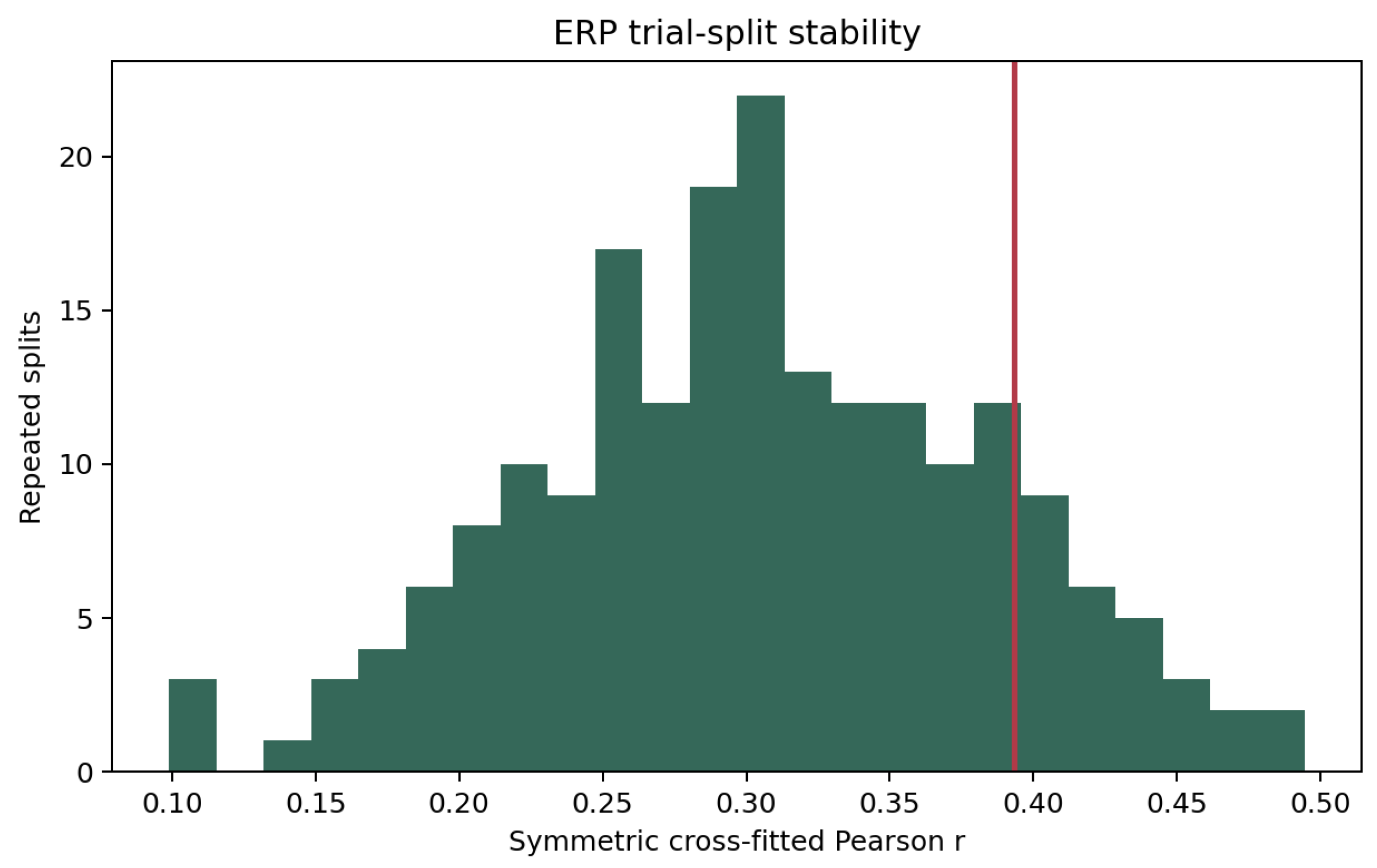
Figure 1. Observer-separated ERP recovery across the locked trial allocation and 200 repeated allocations. Timing and localization are estimated from disjoint trial halves; repeated allocations are dependent stability checks of the same estimand.

Figure 1. Observer-separated ERP recovery across the locked trial allocation and 200 repeated allocations. Timing and localization are estimated from disjoint trial halves; repeated allocations are dependent stability checks of the same estimand.

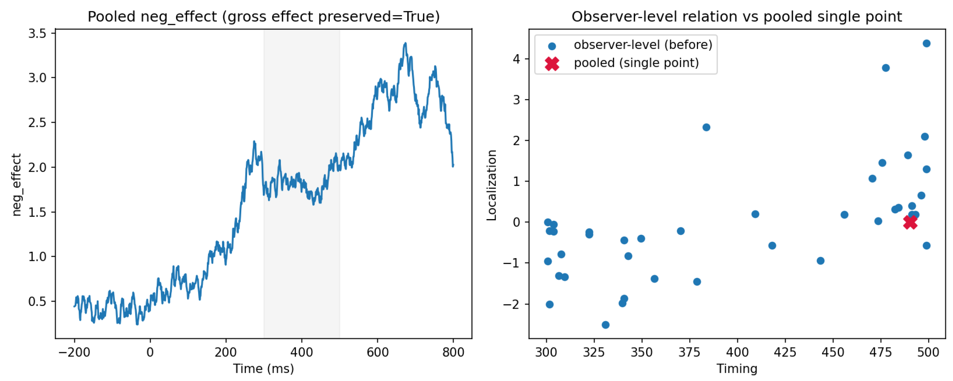
5.2. Pooling Preserves the N400 and Makes the Observer Relation Unavailable

The pooled waveform retained the canonical semantic-negativity effect. Expected and unexpected conditions continued to differ over the familiar N400 interval, and the group profile preserved the broad timing and polarity of the response.

It could not retain timing–localization covariance because pooling removed the observer coordinate on which that relation was defined.

Before pooling, the analysis contained 40 participant-specific timing estimates and 40 corresponding localization estimates. After pooling, it contained one group waveform. Peak timing and early–late allocation could still be described for that waveform, but there was no longer a set of observer pairs across which their covariance could be estimated.

Pooling did not reduce the precision of the estimand. It eliminated the estimand.

A canonical group effect and a structured observer relation can coexist, and an aggregation procedure can preserve the first while removing the coordinate required by the second. The observer relation is not a noisier version of the group effect waiting to be recovered from the average. It is a different scientific object whose defining coordinate is participant identity.

Figure 2. Pooling preserves the group semantic-negativity surface while removing participant-indexed pairs. The pooled waveform answers a population-level question but cannot identify the between-observer timing–localization covariance.

Figure 2. Pooling preserves the group semantic-negativity surface while removing participant-indexed pairs. The pooled waveform answers a population-level question but cannot identify the between-observer timing–localization covariance.

5.3. Desynchronization and Gradient Erasure Collapse Same-Profile Operator Recovery

The primary cross-fit establishes that the relation survives trial separation. The auxiliary same-profile diagnostics ask whether operator-family recovery also requires intact temporal organization.

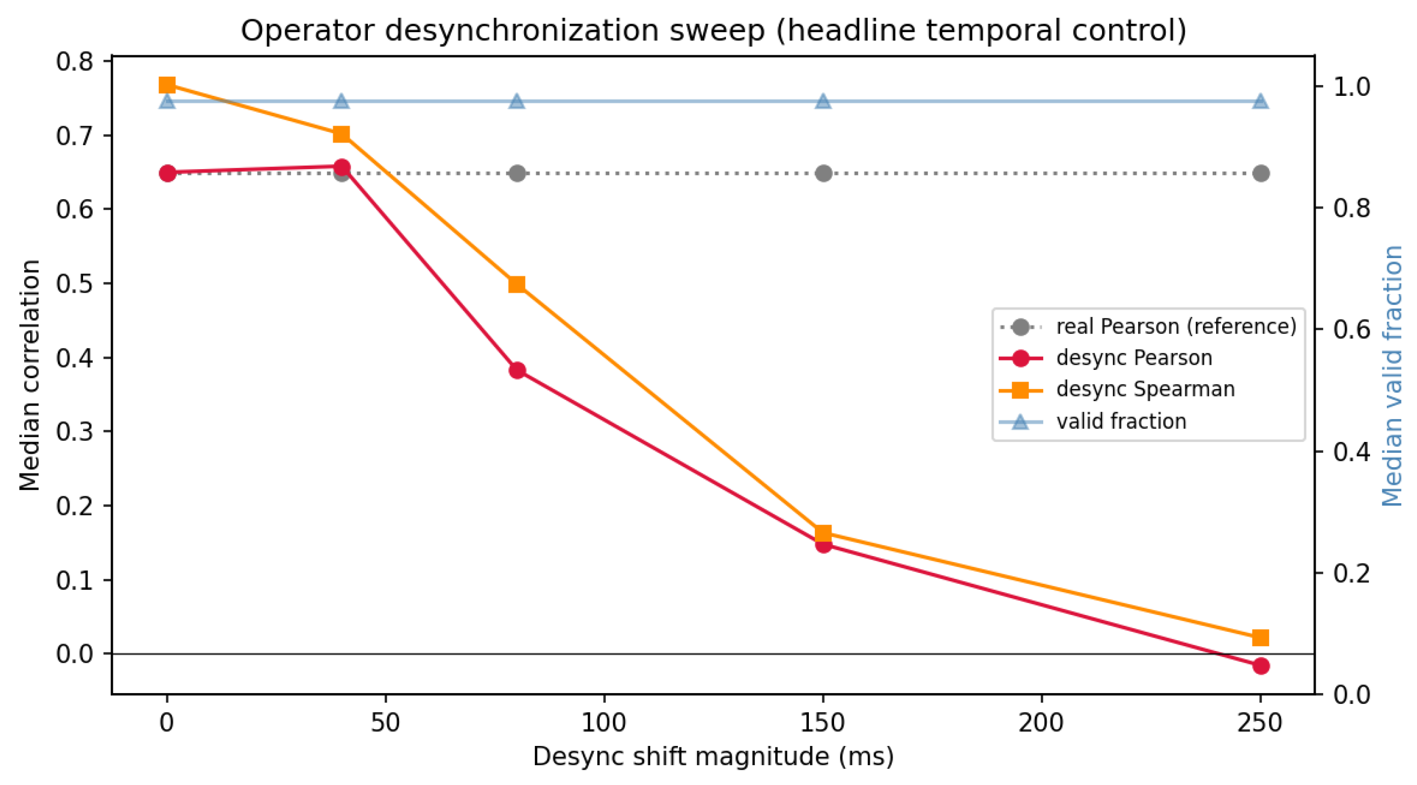
Desynchronization displaced timing and localization operators by $\pm 250$ ms while preserving participant identity, measured amplitudes, trial structure, and the underlying ERP records. The aligned formula-distinct operator-family median of approximately $r=.620$ fell to $r=.005$, with predicted-direction preservation falling to approximately 31.9 percent.

The values remained in the dataset. The participants remained correctly identified. What disappeared was the original temporal correspondence between the two operators.

Temporal-gradient erasure attacked a different property. Within the strict-window family, the median relation fell from approximately $r=.638$ to $r=.010$ after first-order temporal-gradient structure was removed.

Auxiliary same-profile operator recovery collapsed under desynchronization and temporal-gradient erasure, supporting the role of alignment and first-order temporal organization on the tested operator surface.

These controls target structure rather than amplitude alone. A generic response-strength account does not predict that shifting the temporal correspondence or removing the early-to-late gradient should eliminate same-profile operator recovery while leaving participant identity and much of the measured signal intact. The diagnostics support organized temporal structure on that tested surface.

Figure 3. Auxiliary same-profile operator-family recovery across temporal displacement. This diagnostic tests alignment on the same-profile surface and does not directly recompute the locked disjoint cross-fit statistic.

Figure 3. Auxiliary same-profile operator-family recovery across temporal displacement. This diagnostic tests alignment on the same-profile surface and does not directly recompute the locked disjoint cross-fit statistic.

5.4. ERP Recovery Survives Removal of Zero Rectification

The primary ERP surface reverses the unexpected-minus-expected contrast and sets values below zero to zero. The secondary sensitivity retained the polarity reversal and removed only the zero floor.

Observer-paired recovery remained positive on the unrectified surface:

$$r=.330,95\%\mathrm{CI}=[.060,.561],p_{\mathrm{pair}}=.0026.$$

The corresponding amplitude-controlled estimate was $r=.400$.

The amplitude-controlled estimate is descriptive; it was not assigned a separate interval or pairing test.

The relation also recurred across alternative trial allocations. Across 200 repeated splits, the unrectified native median was $r=.332$, with first and third quartiles of $[.269,.390]$; every estimate was positive.

The rectified native estimate was $r=.393$, compared with $r=.330$ without rectification. The paired rectified-minus-unrectified contrast was $\Delta z=.073$, with a two-sided participant-bootstrap interval of $[-.081,.250]$.

The rectified point estimate was larger, but the paired interval crossed zero. Rectification is therefore not required for ERP recovery; the comparison does not establish equivalence between surfaces.

5.5. Repeated Allocations Show Recurrence Across Trial Partitions

The locked trial split was not a uniquely favorable allocation.

Across 200 additional condition-stratified splits, the median symmetric Pearson relation on the primary rectified surface was $r=.305$, with first and third quartiles of $[.256,.361]$. All 200 estimates were positive.

The repeated allocations reuse the same participants and trials. They are not independent replications and do not enlarge the participant sample. Their purpose is narrower: they show that the result is not tied to one convenient assignment of trials to halves.

The locked estimate of $r=.393$ lies above the repeated-split median but within the observed allocation distribution. Recovery therefore varies with trial composition while retaining its direction across admissible splits.

5.6. Amplitude Control

The amplitude-controlled directional estimates were $r_{A\to B}=.449$ and $r_{B\to A}=.413$, producing a symmetric estimate of $r=.431$.

The point estimate remained close to the primary observer-paired relation after timing and localization were residualized against their corresponding half-specific amplitude covariates.

The amplitude-controlled estimate is descriptive; it was not assigned a separate interval or pairing test.

The result narrows a direct magnitude explanation. The relation is not absorbed by the declared linear amplitude terms. It does not establish that waveform morphology, signal quality, or every magnitude-related property is irrelevant.

Table 3. Primary ERP reconstruction and sensitivity results.

Analysis	$\mathit{A}\to \mathit{B}$	$\mathit{B}\to \mathit{A}$	Symmetric estimate	Interval or distribution	Pairing probability	Status
Primary Pearson	.442	.343	.393	[.207, .554]	.0004	Locked primary
Primary Spearman	.458	.367	.413	Secondary rank summary	NA	Locked secondary metric
Amplitude controlled	.449	.413	.431	Descriptive	NA	Descriptive
Repeated splits	NA	NA	Median .305	IQR [.256, .361]; 200 positive splits	NA	Dependent stability
Unrectified Pearson	NA	NA	.330	[.060, .561]	.0026	Prospectively specified secondary
Unrectified amplitude controlled	NA	NA	.400	Descriptive	NA	Descriptive
Unrectified repeated splits	NA	NA	Median .332	IQR [.269, .390]; 200 positive splits	NA	Dependent stability
Rectified minus unrectified	NA	NA	$\Delta z=.073$	[-.081, .250]	NA	Paired surface comparison

Table 3. Primary ERP reconstruction and sensitivity results.

Analysis	$\mathit{A}\to \mathit{B}$	$\mathit{B}\to \mathit{A}$	Symmetric estimate	Interval or distribution	Pairing probability	Status
Primary Pearson	.442	.343	.393	[.207, .554]	.0004	Locked primary
Primary Spearman	.458	.367	.413	Secondary rank summary	NA	Locked secondary metric
Amplitude controlled	.449	.413	.431	Descriptive	NA	Descriptive
Repeated splits	NA	NA	Median .305	IQR [.256, .361]; 200 positive splits	NA	Dependent stability
Unrectified Pearson	NA	NA	.330	[.060, .561]	.0026	Prospectively specified secondary
Unrectified amplitude controlled	NA	NA	.400	Descriptive	NA	Descriptive
Unrectified repeated splits	NA	NA	Median .332	IQR [.269, .390]; 200 positive splits	NA	Dependent stability
Rectified minus unrectified	NA	NA	$\Delta z=.073$	[-.081, .250]	NA	Paired surface comparison

6. Results II: Reader-Paired Temporal Organization Across Signed and Clipped Behavioral Surfaces

The locked clipped concentration family recovers a positive but heterogeneous reader relation. Signed temporal-allocation operators reveal a much stronger and more consistent organization.

6.1. The Locked Clipped Concentration Family

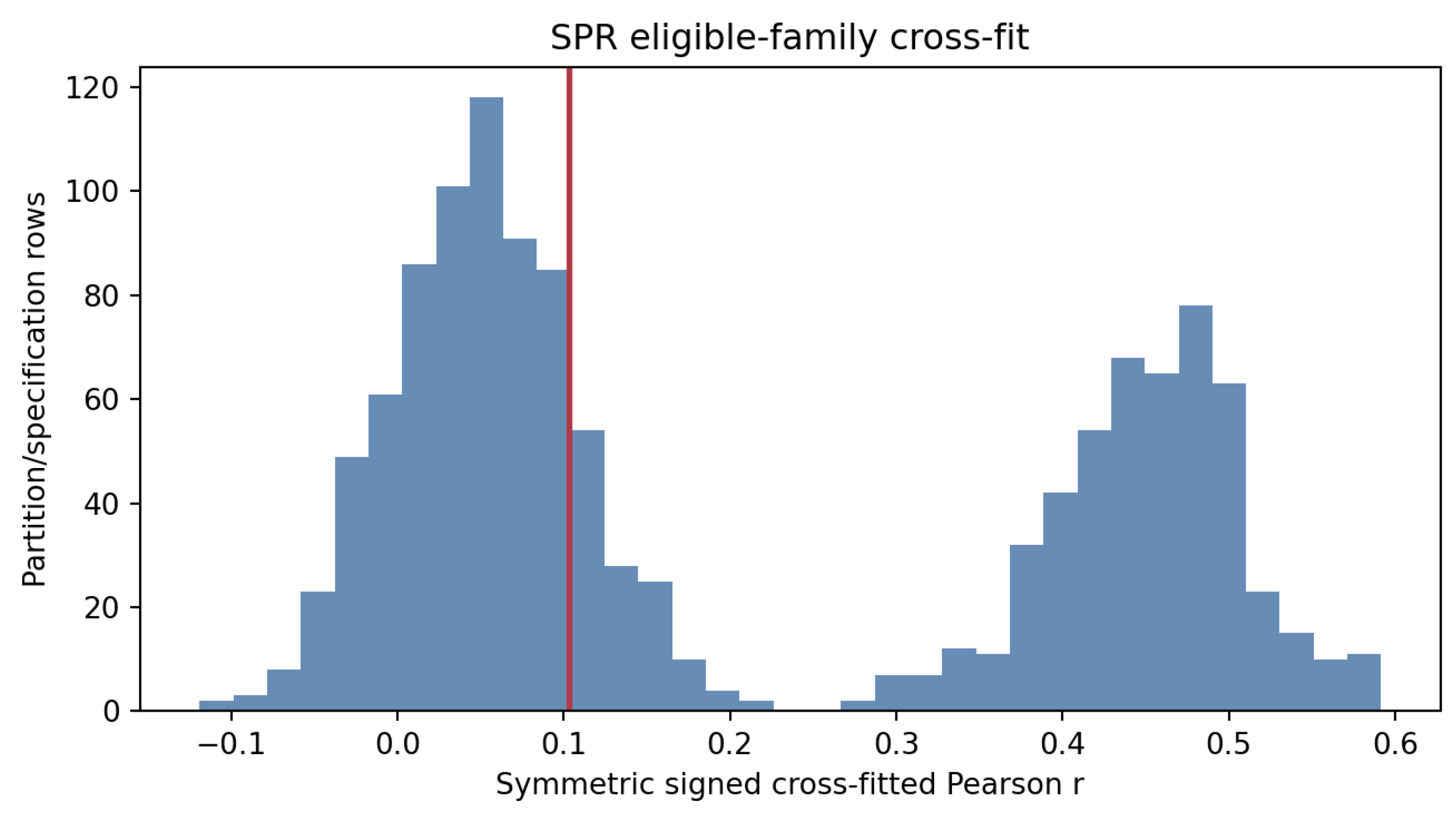
The locked Natural Stories analysis recovered a positive reader-paired relation across the clipped concentration family:

$$r=.103,95\%\mathrm{CI}=[-.026,.297],p_{\mathrm{pair}}=.0162,$$

with 88.88 percent predicted-direction preservation.

Correct reader pairing therefore carried behavioral structure above random reassignment, while uncertainty under reader sampling remained substantial. The two summaries answer different questions: the pairing permutation tests whether recovery depends on correct reader correspondence, and the bootstrap interval characterizes variation under reader resampling.

The family contained 1,250 symmetric estimates across 125 scored story partitions and ten eligible specifications. These estimates are dependent. They reuse readers, stories, partitions, lag slopes, and operator components. The family median summarizes recurrence across the declared clipped surface. It is not an average of 1,250 independent effects.

The clipped result was also heterogeneous across operators. Some timing–concentration pairs carried a clearer positive relation than others, and the family did not support a single uniform effect size across all constructions. That heterogeneity is part of the result. The locked surface recovers reader organization, but it compresses signed lag structure into nonnegative concentration and does not expose every form of temporal allocation equally well.

Descriptively, this heterogeneity was structured rather than diffuse. The four location-sensitive peak-lag specifications were positive across all 125 scored partitions, with median relations from $r=.416$ to $r=.497$. The six general cost-concentration specifications were substantially weaker, with medians from $r=.020$ to $r=.099$ (Supplementary Appendix F.4). The locked family median therefore combines a strong location-sensitive block with a much weaker general concentration block.

The clipped family establishes the primary locked result. The signed-safe analysis then shows that a different temporal surface carries substantially stronger organization.

Figure 4. Locked clipped-concentration recovery across the dependent Natural Stories specification family. Family inference uses a shared reader-pairing null; overlapping partitions and specifications are not treated as independent replications.

Figure 4. Locked clipped-concentration recovery across the dependent Natural Stories specification family. Family inference uses a shared reader-pairing null; overlapping partitions and specifications are not treated as independent replications.

6.2. Clipping Affects a Minority of Valid Profiles

The clipping audit contained 48,218 fully valid three-position profiles. Clipping changed no position in 85.61 percent of profiles, one position in 12.86 percent, and two positions in 1.53 percent. It never changed all three positions, and no fully valid profile had a nonpositive clipped total. Clipping therefore affected a minority of the profile population.

Table 4. Clipping prevalence among fully valid Natural Stories profiles.

Clipped positions	Profiles	Percent
0	41,280	85.61%
1	6,200	12.86%
2	738	1.53%
3	0	0.00%
Total	48,218	100.00%

Table 4. Clipping prevalence among fully valid Natural Stories profiles.

Clipped positions	Profiles	Percent
0	41,280	85.61%
1	6,200	12.86%
2	738	1.53%
3	0	0.00%
Total	48,218	100.00%

6.3. Signed Temporal-Allocation Operators Reveal Strong Recovery

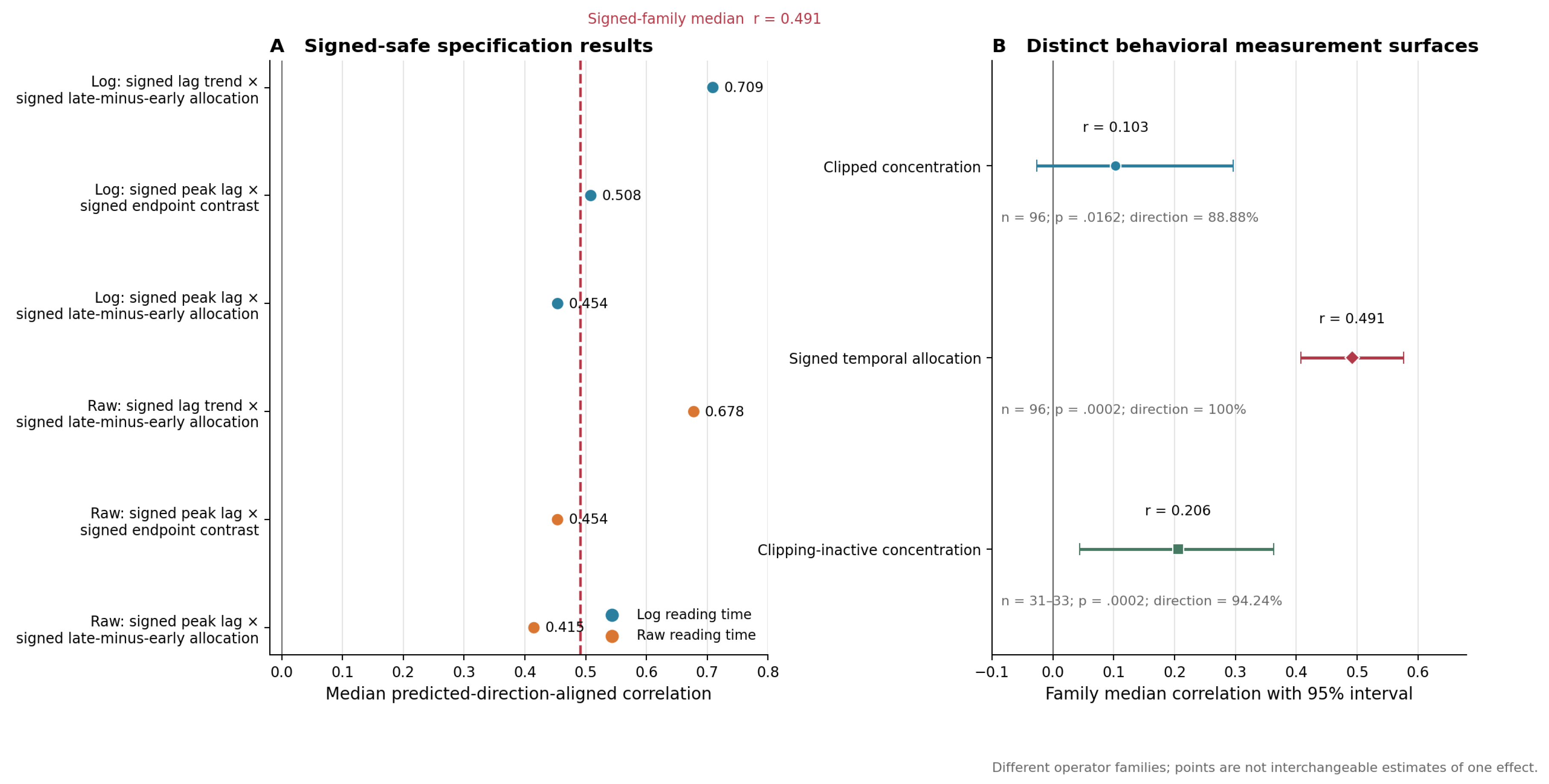
Every signed-safe specification was positive, with specification medians ranging from approximately $r=.415$ to $r=.709$. The family result was

$$r=.491,95\%\mathrm{CI}=[.407,.577],p_{\mathrm{pair}}=.0002,$$

with 100 percent predicted-direction preservation.

The result was not carried by one unusually strong operator pair. All six specifications supported the predicted direction, and even the weakest specification produced a substantial positive median.

Across the full dependent family, all 750 predicted-direction-aligned partition-specification estimates were positive. Because these estimates share readers, stories, partitions, and operator components, this represents complete directional recurrence across the 125 scored complementary story allocations rather than 750 independent replications. The strongest relation paired continuous signed lag trend with signed late-minus-early allocation under both log and raw reading time, with median $r=.709$ and $r=.678$, respectively (Supplementary Appendix C.11). Signed recovery was therefore not confined to a discrete peak estimator or a single reading-time transformation.

The signed-safe operators preserve temporal direction across the current word and downstream positions. They retain whether surprisal-linked reading-time structure shifts earlier or later, rather than converting the lag profile into nonnegative mass before temporal organization is measured.

Retaining temporal direction exposed reader-paired organization more clearly than reducing lag structure to nonnegative concentration.

The contrast compares distinct operator families. The signed family uses peak position, signed lag trend, signed early–late allocation, and signed endpoint contrast. The locked family uses normalized concentration operators defined on nonnegative profiles. The two families measure related but distinct properties.

The result changes the behavioral interpretation. Natural Stories contains strong and consistent reader-paired temporal organization when the measurement surface preserves signed allocation.

Figure 5. Signed temporal-allocation operators reveal the strongest reader-paired behavioral organization. Panel A shows the six prospectively specified signed-safe specification medians, all of which are positive. Panel B compares the family-level results across the locked clipped concentration surface, the signed temporal-allocation surface, and the clipping-inactive selected-profile diagnostic. The signed family produces the strongest and most consistent recovery. The three rows represent different operator families and should not be interpreted as interchangeable estimates of one effect.

Figure 5. Signed temporal-allocation operators reveal the strongest reader-paired behavioral organization. Panel A shows the six prospectively specified signed-safe specification medians, all of which are positive. Panel B compares the family-level results across the locked clipped concentration surface, the signed temporal-allocation surface, and the clipping-inactive selected-profile diagnostic. The signed family produces the strongest and most consistent recovery. The three rows represent different operator families and should not be interpreted as interchangeable estimates of one effect.

6.4. The Nonnegative Relation Recurs Where Clipping Is Inactive

The no-clipping diagnostic returned to the original nonnegative operator family and retained only profiles for which clipping performed no transformation.

The clipping-inactive common-reader strata contained 31 to 33 readers, depending on the partition family. Within those strata, the result was

$$r=.206,95\%\mathrm{CI}=[.044,.363],p_{\mathrm{pair}}=.0002,$$

with 94.24 percent predicted-direction preservation.

The original nonnegative concentration relation therefore recurs in profiles that were already nonnegative before the clipping rule was applied. Clipping is not required to produce that relation.

This selected-profile diagnostic uses substantially smaller strata than the locked 96-reader sample because inclusion depends on the observed sign structure of each reader profile. It does not replace the population-wide locked result.

Its role is specific: where clipping was inactive, the nonnegative relation remained positive, interval-supported, and dependent on correct reader pairing.

6.5. Behavioral Surface Comparison

The three analyses expose different parts of reader-paired temporal organization.

The locked family measures where nonnegative surprisal-linked processing cost is concentrated across current and downstream positions. It produces a positive but heterogeneous relation.

The signed-safe family preserves whether the reading-time effect moves earlier or later across the lag profile. It produces a strong and consistent relation across every declared specification.

The no-clipping diagnostic returns to the original concentration family in the subset of profiles where clipping changed nothing. It recovers a positive relation under correct reader pairing.

Table 5. Reader-paired recovery across behavioral measurement surfaces.

Behavioral surface	Status	Readers	Specifications	Median r	95% interval	Pairing p	Direction preservation
Clipped concentration	Locked primary	96	10	.103	[-.026, .297]	.0162	88.88%
Signed temporal allocation	Prospectively specified secondary	96	6	.491	[.407, .577]	.0002	100%
Clipping-inactive concentration	Selected-profile diagnostic	31–33	10	.206	[.044, .363]	.0002	94.24%

Table 5. Reader-paired recovery across behavioral measurement surfaces.

Behavioral surface	Status	Readers	Specifications	Median r	95% interval	Pairing p	Direction preservation
Clipped concentration	Locked primary	96	10	.103	[-.026, .297]	.0162	88.88%
Signed temporal allocation	Prospectively specified secondary	96	6	.491	[.407, .577]	.0002	100%
Clipping-inactive concentration	Selected-profile diagnostic	31–33	10	.206	[.044, .363]	.0002	94.24%

Reader-paired temporal organization is strong on the signed allocation surface and positive but heterogeneous on the clipped concentration surface.

7. Results III: Temporal Compression Preserves Observer Recovery

The predicted native-resolution advantage did not appear. Reducing peak timing to three ordered categories preserved observer recovery on both rectified and unrectified surfaces.

7.1. Why Native Timing Was Expected to Matter

The original prediction treated fine temporal precision as part of the structure carrying the ERP relation. Native sampling distinguishes peak latencies separated by less than one millisecond, while a three-bin representation retains only broad early, middle, and late placement.

If the observer relation depended on those fine distinctions, severe temporal compression should weaken recovery. Native timing should therefore produce a stronger relation than three-bin timing.

That prediction was frozen before the compression outcomes were inspected.

7.2. The Frozen Native-Resolution Prediction Failed

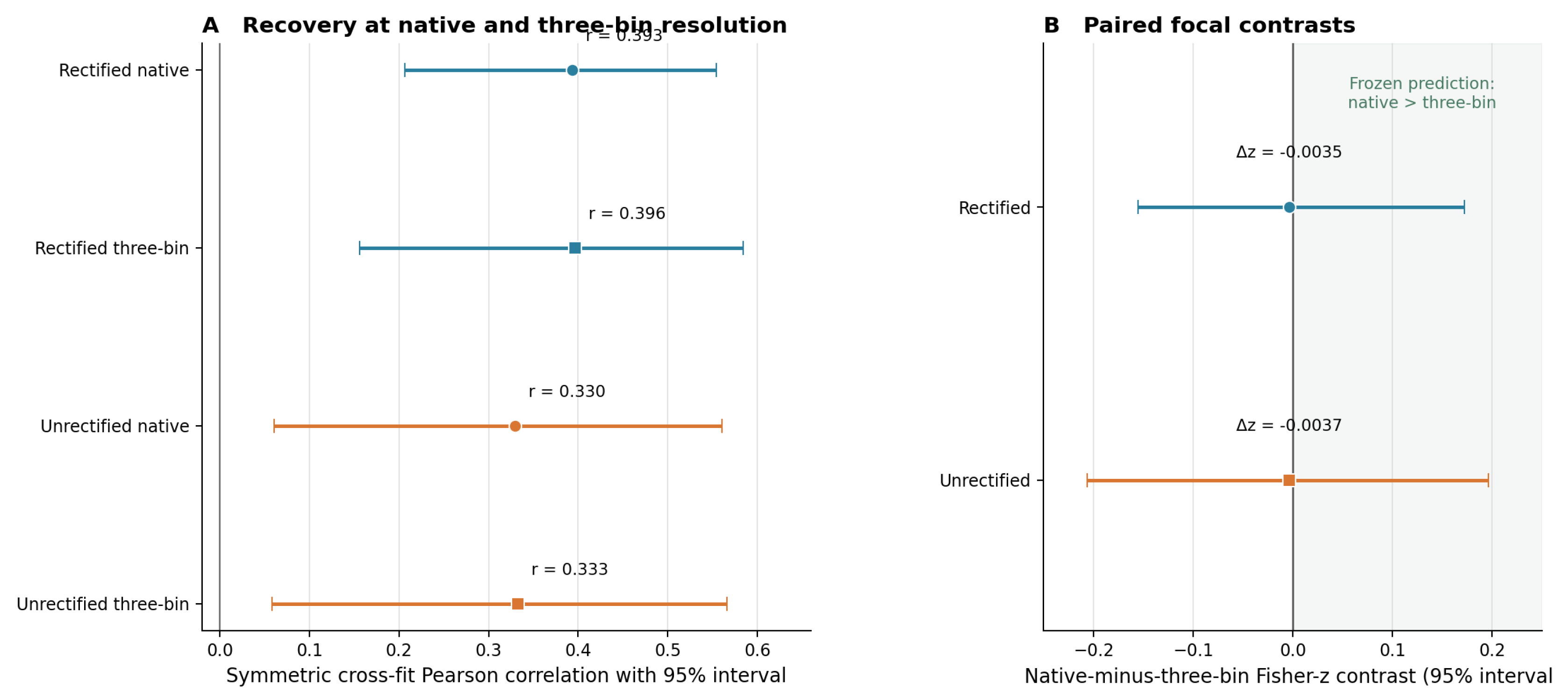
Native recovery was $r=.393$. Three-bin recovery was $r=.396$.

The predicted native-resolution advantage did not appear.

The native-minus-three-bin contrast was $\Delta z\approx -.004$, with a 95 percent observer-bootstrap interval of $[-.155,.172]$ and a one-sided probability of $p=.510$ in the frozen native-greater direction.

The point estimate was slightly opposite the prediction.

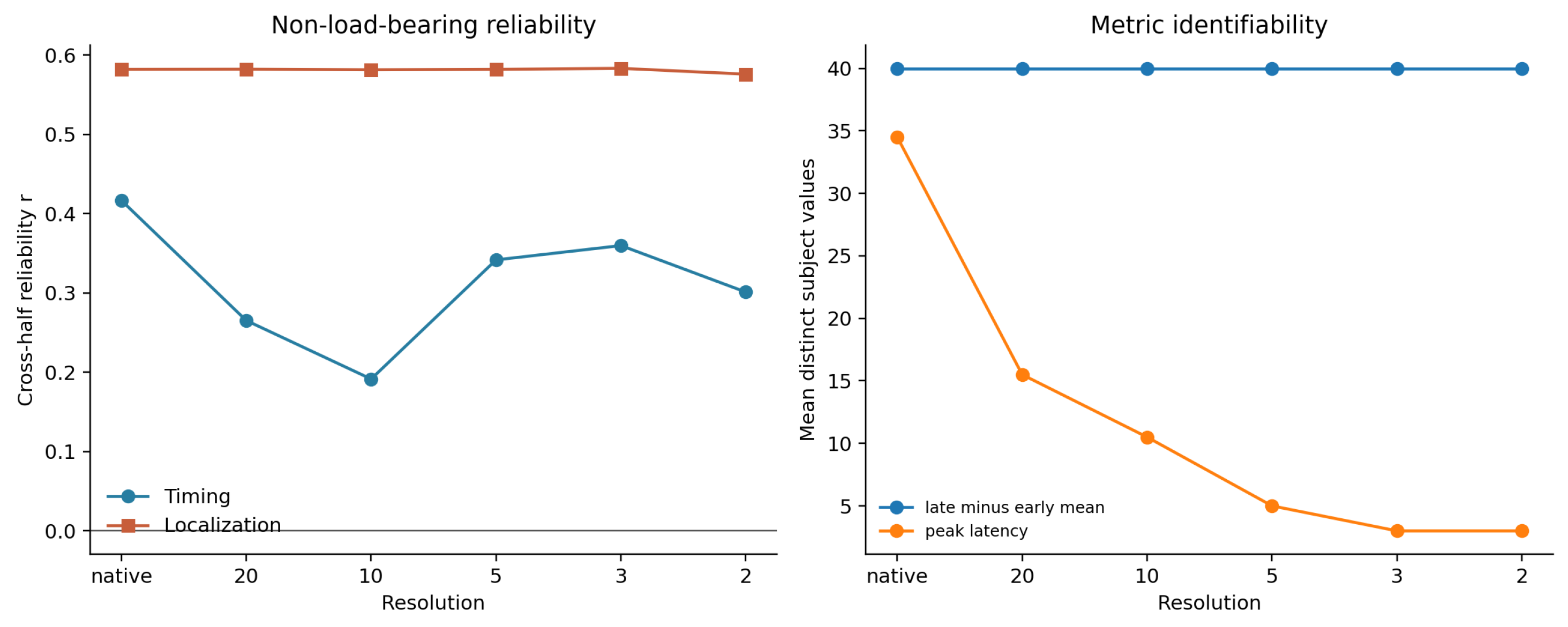
Compression reduced average peak-timing cardinality from approximately 34.5 native values to three ordered categories. Observer-paired recovery remained at the native level.

The interval does not establish equivalence across resolutions. It establishes that the frozen experiment produced no evidence of the predicted native-resolution advantage and no detectable attenuation under the declared three-bin transformation.

Figure 6. Three-bin compression preserves observer recovery on rectified and unrectified ERP surfaces. Native and three-bin recovery are nearly identical on both surfaces. The paired contrasts are close to zero and slightly opposite the prospectively frozen native-greater prediction.

Figure 6. Three-bin compression preserves observer recovery on rectified and unrectified ERP surfaces. Native and three-bin recovery are nearly identical on both surfaces. The paired contrasts are close to zero and slightly opposite the prospectively frozen native-greater prediction.

7.3. Compression Removed Timing Distinctions, Not the Relation

The three-bin operator collapsed many distinct native latencies into the same temporal category. Fine differences among participants were no longer available, and the number of possible timing values fell by more than an order of magnitude.

Broad temporal order remained. Participants could still be distinguished as expressing earlier, middle, or later peak timing. Observer identity also remained intact. Each participant’s compressed timing estimate was still paired with that participant’s independently estimated localization.

Localization changed much less than timing. Three-bin localization correlated approximately $r=.989$ with native localization. The transformation therefore imposed a strong reduction in peak-timing granularity and a weak reduction in the broad early–late localization axis.

Observer recovery persisted under that asymmetric transformation.

This result separates native temporal precision from the relation it was used to estimate. The information required to recover this relation was not identical to native temporal precision.

Compression removed timing distinctions, not the relation.

Figure 7. Metric identifiability declines under temporal compression while observer-paired recovery remains stable. The plot separates the number of timing distinctions available to an estimator from the relation recovered among observers.

Figure 7. Metric identifiability declines under temporal compression while observer-paired recovery remains stable. The plot separates the number of timing distinctions available to an estimator from the relation recovered among observers.

7.4. The Result Survives Without Rectification

The compression result remained after zero rectification was removed. Native recovery was $r=.330$, and three-bin recovery was $r=.333$. The native-minus-three-bin contrast was $\Delta z=-.0037$, with a 95 percent interval of $[-.207,.196]$ and $p=.511$ in the frozen native-greater direction. At three bins, the observer relation remained separated from the shared pairing null, $p=.0024$.

Neither zero rectification nor native timing cardinality is required for the compression result.

The parallel outcome matters because rectification and compression remove different properties. Rectification removes values below zero after polarity orientation. Compression removes fine temporal distinctions. Recovery persists when either operation is absent or severe.

Figure 8. Observer recovery across the prospectively frozen rectified resolution ladder. Three-bin compression sharply reduces timing cardinality while preserving the observer-paired relation.

Figure 8. Observer recovery across the prospectively frozen rectified resolution ladder. Three-bin compression sharply reduces timing cardinality while preserving the observer-paired relation.

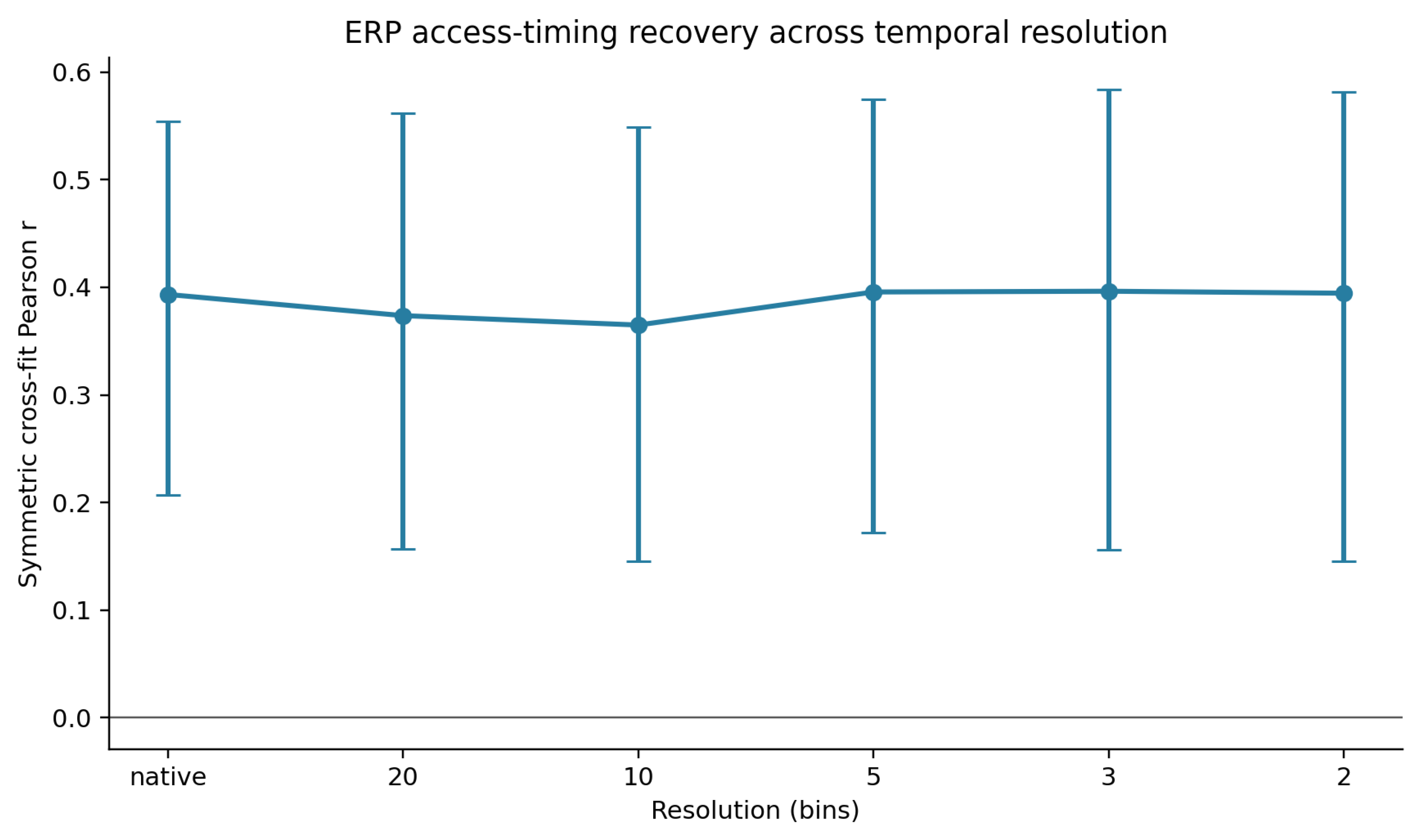
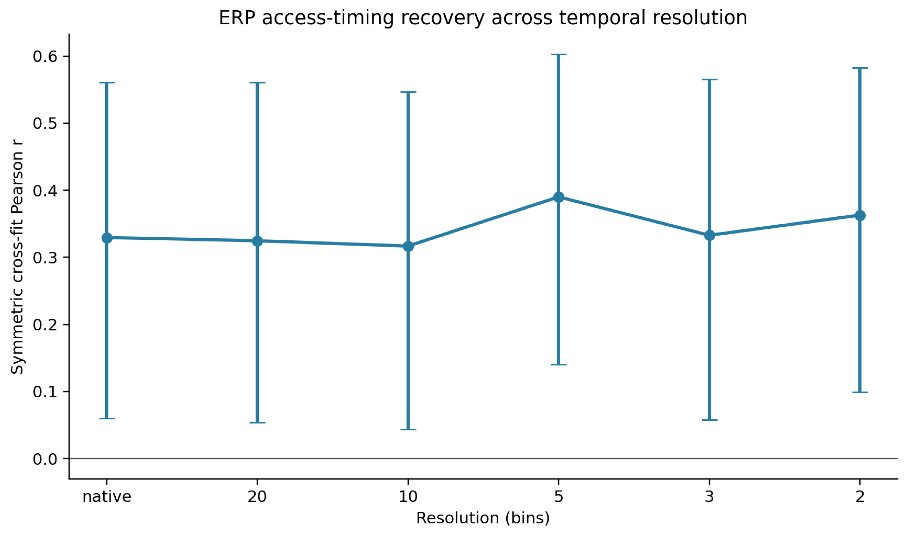
Figure 9. Unrectified observer recovery across the same frozen resolution ladder. Native and three-bin recovery remain nearly identical after the rectification step is removed.

Figure 9. Unrectified observer recovery across the same frozen resolution ladder. Native and three-bin recovery remain nearly identical after the rectification step is removed.

7.5. Full Resolution Ladder and Repeated Allocations

Recovery remained positive across the complete frozen ladder.

Table 6. Observer recovery across the frozen resolution ladder.

Resolution	Rectified r	Unrectified r
Native	.393	.330
20 bins	.374	.325
10 bins	.365	.317
5 bins	.396	.390
3 bins	.396	.333
2 bins	.395	.363

Table 6. Observer recovery across the frozen resolution ladder.

Resolution	Rectified r	Unrectified r
Native	.393	.330
20 bins	.374	.325
10 bins	.365	.317
5 bins	.396	.390
3 bins	.396	.333
2 bins	.395	.363

Full peak-timing cardinality values across the frozen resolution ladder are reported in Supplementary Table D6.

Both ladders were nonmonotonic. The frozen finite-resolution slope on ${log}_{2}K$ was $-.0105$, with a 95 percent interval of $[-.0520,.0394]$ and $p=.643$ in the predicted positive direction. On the unrectified surface, the slope was $-.0134$, with an interval of $[-.0809,.0484]$ and $p=.660$.

No monotonic native-resolution advantage appeared on either surface.

Descriptively, compression survival was not confined to the canonical operator pair. All 10 formula-distinct eligible ERP operator pairs retained their predicted direction at every level of the six-step resolution ladder (Supplementary Appendix D.14). No pair-specific resolution contrast was prospectively designated, so this family-wide pattern supports robustness without enlarging the frozen confirmatory claim.

The repeated-allocation results pointed in the same direction. Across 200 alternative splits, median rectified recovery was $r=.305$ at native resolution and $r=.343$ at three bins. The median native-minus-three-bin contrast was $-.035$, and native recovery exceeded three-bin recovery in 24.5 percent of splits. On the unrectified surface, the corresponding medians were $r=.332$ and $r=.356$.

The repeated allocations reuse the same participants and trials. They do not create additional independent experiments. They show that compression survival is not tied to the locked trial split.

7.6. Tie-Handling Sensitivities

One participant produced a flat native profile with exact peak ties in both trial halves. Two post-diagnostic sensitivities either excluded that participant or assigned the native profile its mean tied location. Both contrasts remained near zero. Supplementary Appendix D reports the full estimates and participant-level diagnostics.

8. Discussion: Relational Observability and What the Transformations Reveal

The experiments sharpened ODER through a split theoretical outcome. Observer-indexed temporal organization recurred through correct identity across disjoint observations, supporting the theory’s central empirical prediction. Native timing did not outperform three-bin timing, rejecting the frozen resolution prediction and changing the proposed carrier of the relation. The experiments separate properties that are often treated as one: observer identity, temporal alignment, timing cardinality, sign, order, and concentration. Their effects on recovery were sharply different. Some transformations removed large amounts of detail and preserved the relation. Others retained detailed signals and destroyed the coordinates required to estimate it.

8.1. The Preservation Map

Table 7 summarizes what each tested surface or transformation preserved and what happened to observer-paired recovery.

In the table, Preserved indicates preservation, Removed indicates removal, and ∼ indicates partial preservation or preservation only at the marginal level.

Table 7. Coordinates preserved by the tested measurement transformations.

Surface or transformation	Observer identity	Temporal order or alignment	Sign	Native cardinality	Concentration	Observer relation	Interpretation
Native observer-paired ERP	Preserved	Preserved	Removed	Preserved	Preserved	Recovered	Primary rectified relation
Observer reassignment	Removed	Preserved	Removed	Preserved	Preserved	Collapsed	Correct correspondence is required
Pooling	Removed	Preserved at group level	Removed	Preserved	Preserved at group level	Unavailable	Participant axis removed
Desynchronization	Preserved	Removed	Removed	Preserved	∼	Same-profile collapse	Cross-operator temporal alignment removed
Temporal-gradient erasure	Preserved	Removed	Removed	Preserved	∼	Same-profile collapse	First-order temporal shape removed
Three-bin ERP compression	Preserved	Preserved at broad scale	Removed	Removed	Preserved	Recovered	Fine timing distinctions removed
Unrectified ERP	Preserved	Preserved	Preserved	Preserved	Not applicable	Recovered	Zero floor removed
Signed behavioral allocation	Preserved	Preserved	Preserved	Not applicable	Removed	Strongly recovered	Temporal direction retained
Clipped behavioral concentration	Preserved	Preserved	Removed	Not applicable	Preserved	Recovered, heterogeneous	Direction converted to nonnegative mass
Clipping-inactive behavioral profiles	Preserved	Preserved	Preserved within selected profiles	Not applicable	Preserved	Recovered	Original relation recurs without active clipping

Table 7. Coordinates preserved by the tested measurement transformations.

Surface or transformation	Observer identity	Temporal order or alignment	Sign	Native cardinality	Concentration	Observer relation	Interpretation
Native observer-paired ERP	Preserved	Preserved	Removed	Preserved	Preserved	Recovered	Primary rectified relation
Observer reassignment	Removed	Preserved	Removed	Preserved	Preserved	Collapsed	Correct correspondence is required
Pooling	Removed	Preserved at group level	Removed	Preserved	Preserved at group level	Unavailable	Participant axis removed
Desynchronization	Preserved	Removed	Removed	Preserved	∼	Same-profile collapse	Cross-operator temporal alignment removed
Temporal-gradient erasure	Preserved	Removed	Removed	Preserved	∼	Same-profile collapse	First-order temporal shape removed
Three-bin ERP compression	Preserved	Preserved at broad scale	Removed	Removed	Preserved	Recovered	Fine timing distinctions removed
Unrectified ERP	Preserved	Preserved	Preserved	Preserved	Not applicable	Recovered	Zero floor removed
Signed behavioral allocation	Preserved	Preserved	Preserved	Not applicable	Removed	Strongly recovered	Temporal direction retained
Clipped behavioral concentration	Preserved	Preserved	Removed	Not applicable	Preserved	Recovered, heterogeneous	Direction converted to nonnegative mass
Clipping-inactive behavioral profiles	Preserved	Preserved	Preserved within selected profiles	Not applicable	Preserved	Recovered	Original relation recurs without active clipping

The pattern is not ordered by the quantity of detail retained. Pooling preserves a detailed group waveform and eliminates the relation. Three-bin compression preserves only broad timing categories and retains it. The relevant distinction is structural: which coordinates remain available after the operator acts.

8.2. Pooling and Compression Are Complementary Results

Pooling retained the detailed group waveform and made the observer relation unavailable. Three-bin compression discarded most native timing distinctions and preserved it.

These are complementary results because the two transformations act on different coordinates.

Pooling operates across observers. It combines participant-level profiles into one group representation. The full sampled waveform remains, and the canonical semantic-negativity effect remains visible. Observer identity does not survive the operation. The covariance object therefore disappears even though temporal detail remains abundant.

Compression operates within observers. It maps many native peak latencies onto three ordered categories. Fine timing distinctions disappear, but each participant remains identifiable and each compressed timing estimate remains paired with that participant’s independently estimated localization. The observer relation survives.

Three-bin compression produced relation-preserving information loss. Most native peak-timing distinctions disappeared, yet the observer relation remained recoverable. Pooling produced the opposite pattern: a detailed group waveform remained while the observer relation became unavailable. Information quantity alone therefore cannot rank these transformations.

Coordinate identifiability and relational recoverability are different measurement properties. More temporal detail did not preserve the relation; preserving the observer did.

The pooling–compression contrast therefore raises a pre-analysis question: does the retained dataset preserve the coordinates needed to construct the observer-level relation at all? The retained representation must preserve joint observer linkage, support a resolved or constructible temporal or positional surface, provide disjoint estimation data, and permit timing and localization to be estimated through separately estimable, nonredundant operators.

These requirements impose an order on inference: measurability precedes detectability. If they are not satisfied, the relation has not been tested rather than found absent. Appendix A.1 formalizes this pre-analysis eligibility test as Tier 0. Data-release adequacy is therefore relation-specific: preprocessed or derived data may qualify when the required coordinates remain jointly linkable, while detailed summaries may not if observer identity or temporal structure has been collapsed.

8.3. Sign and Concentration Expose Different Behavioral Structures

The Natural Stories analyses separate two ways of representing temporal organization.

The clipped concentration surface begins with surprisal-linked lag slopes and sets negative values to zero. The resulting profile represents nonnegative processing mass across current and downstream positions. Its operators measure where that mass is concentrated.

This surface carries reader organization. The locked family produces a positive median relation and exceeds the shared reader-pairing null. Its strength varies across operator pairs, and its family interval crosses zero.

The signed allocation surface retains the direction of the lag slopes. Negative and positive values remain distinct. The operators measure whether processing structure moves earlier or later, whether late positions exceed early positions, and how the profile changes across its endpoints.

This surface carries the relation much more strongly. Every signed-safe specification is positive. The family median is $r=.491$, compared with $r=.103$ on the locked clipped surface, and predicted-direction preservation rises from 88.88 percent to 100 percent.

The comparison is not a contest between two settings of the same estimator. Concentration and allocation are different measurement objects. Concentration asks where nonnegative magnitude accumulates. Signed allocation asks how temporally directed structure is distributed.

Both carry reader organization. Signed allocation carries it more strongly.

8.4. What Appears to Be Preserved

Across the tested transformations, recovery tracked a small set of structural properties.

8.4.1. Observer Identity

The relation requires a mapping between the timing estimate and localization estimate belonging to the same observer. Observer reassignment breaks that mapping. Pooling removes the observer axis entirely. In both cases, recovery disappears.

8.4.2. Temporal Ordering and Alignment

Three-bin compression preserves broad early-to-late order, and the relation survives. Desynchronization breaks the original correspondence between temporal estimates, and auxiliary same-profile operator recovery collapses. The distinction is not simply whether time remains present. It is whether the relevant temporal organization remains aligned.

8.4.3. Relative Early–Late Placement

The primary ERP localization measure compares late and early semantic-negativity allocation. Three-bin compression leaves that broad division largely intact. Three-bin localization correlates approximately $r=.989$ with native localization, even though peak-timing cardinality is sharply reduced.

This suggests that relative temporal placement carries more of the relation than millisecond-level peak differentiation.

8.4.4. Signed Allocation

The strongest Natural Stories recovery appears when temporal direction is retained. Signed lag trend, signed endpoint contrast, and signed early–late allocation expose stable reader organization that is weaker on the magnitude-only concentration surface.

8.4.5. Broad Localization

Both ERP and Natural Stories recover relations between a timing coordinate and a broader localization or allocation coordinate. The exact operators differ, but both preserve information about where temporal structure is expressed relative to an early–late axis.

The experiments isolate a preservation class. They do not identify one unique carrier. Observer identity, temporal alignment, broad order, relative placement, and signed allocation remain viable components of the relation. Their separate contributions now require controlled comparison.

8.5. Relational Observability Principle

A measurement operator is adequate for a relational claim only when it preserves the coordinates required to estimate that relation. Loss of detail and loss of relation are different transformations. An operator can discard many values while preserving a relation, or retain a detailed signal while eliminating the relation’s defining coordinate.

Relational observability concerns scientific representation before it concerns estimator choice. A multivariate hierarchical model, latent-variable model, or another inferential framework may estimate the same observer relation once the relevant coordinates have been specified. The prior question is which quantities must be constructed and which coordinates must remain available for that relation to exist as an estimable object.

In this sense, observer-level relational construction and aggregation are generally noncommuting operations for relations defined through observer identity.

Failure to recover a relation can arise because the estimate is noisy, because the relevant coordinates have been distorted, or because a defining coordinate has been removed. Pooling produces the third failure for the observer-indexed relation examined here.

Let

$${\mathcal{S}}_i$$

denote the measured state or data surface for observer i.

Let $M_T$ be a timing operator and $M_L$ a localization or allocation operator. The observer-level quantities are

$$T_i=M_T\left({\mathcal{S}}_i\right)$$

and

$$L_i=M_L\left({\mathcal{S}}_i\right).$$

The declared observer relation is

$$R=Rel\left({\left\{T_i\right\}}_{i=1}^N,{\left\{L_i\right\}}_{i=1}^N\right),$$

where Rel denotes the declared relational statistic, here usually correlation after predicted-direction alignment and symmetric cross-fit aggregation.

Now let Q be a measurement transformation. The transformed observer surface is

$${\mathcal{S}}_i^{\left(Q\right)}=Q\left({\mathcal{S}}_i\right),$$

and the transformed relation is

$$R_Q=Rel\left({\left\{M_T\left({\mathcal{S}}_i^{\left(Q\right)}\right)\right\}}_{i=1}^N,{\left\{M_L\left({\mathcal{S}}_i^{\left(Q\right)}\right)\right\}}_{i=1}^N\right).$$

The relation is observable under Q when three conditions hold:

1.

the transformed surface retains the observer index i;

2.

the transformed operators remain defined;

3.

correct observer pairing continues to recover the declared relation above reassignment.

Three-bin compression satisfies these conditions. It transforms each observer’s surface separately, preserves the index i, and retains enough temporal structure for $R_Q$ to remain recoverable.

Pooling does not. It acts on the set of observer surfaces:

$$Q_{\mathrm{pool}}\left({\left\{{\mathcal{S}}_i\right\}}_{i=1}^N\right)=\overline{\mathcal{S}}.$$

The output is one pooled surface rather than an indexed family. The quantities $T_i$ and $L_i$ no longer exist as observer-level pairs, so the relation is unavailable.

Desynchronization preserves i but breaks temporal correspondence. Gradient erasure preserves i but removes the temporal structure required by the operators. Rectification removes sign but leaves enough organization for recovery. Clipping removes temporal direction and weakens the behavioral relation without creating it.

Relational observability is therefore operator-specific. It asks whether the transformation preserves the coordinates needed by the declared relation.

8.6. What This Changes for Linguistics

The immediate implications concern ERP and self-paced reading. Grand-average component scoring remains valuable for population effects, while participant-specific peak timing, onset, centroid, area, and early–late allocation require operator-defined measurement and observer-level reliability. Disjoint estimation tests whether their relations recur beyond one waveform; temporal transformations identify which features carry them. Coarse timing should therefore be evaluated by the relation it preserves rather than dismissed through resolution alone.

For self-paced reading, current-word and spillover effects form a temporal allocation profile. Reader exposure, story history, and partition structure must remain explicit when those profiles are constructed. The signed results show that the direction of current-to-spillover change carries stronger reader organization than the clipped concentration surface.

The same measurement question extends to fixation and regression timing in eye tracking, onset and concentration in pupillometry, and alignment across speakers and listeners in continuous speech [1,5,18,21]. These are prospective applications of the relational design. In each domain, observer identity, temporal order, and event alignment should be preserved before the relation is estimated.

Individual timing cannot be classified as nuisance variance before testing whether it carries stable observer relations.

Table 8. Field implications of relational timing.

Domain	Common population object	Candidate observer relation	Transformation risk
ERP	Grand-average component	Latency with temporal localization	Pooling, desynchronization, morphology-sensitive scoring
Self-paced reading	Mean current-word or spillover cost	Reader timing with signed lag allocation	Reader pooling, clipping, uneven exposure
Eye tracking	Mean fixation or regression effect	Fixation timing with early–late allocation	Event averaging, temporal warping
Pupillometry	Mean dilation profile	Onset or peak timing with concentration	Participant averaging, smoothing
Speech and auditory processing	Mean acoustic or neural alignment	Speaker- or listener-specific timing relations	Cross-speaker pooling, alignment loss

Table 8. Field implications of relational timing.

Domain	Common population object	Candidate observer relation	Transformation risk
ERP	Grand-average component	Latency with temporal localization	Pooling, desynchronization, morphology-sensitive scoring
Self-paced reading	Mean current-word or spillover cost	Reader timing with signed lag allocation	Reader pooling, clipping, uneven exposure
Eye tracking	Mean fixation or regression effect	Fixation timing with early–late allocation	Event averaging, temporal warping
Pupillometry	Mean dilation profile	Onset or peak timing with concentration	Participant averaging, smoothing
Speech and auditory processing	Mean acoustic or neural alignment	Speaker- or listener-specific timing relations	Cross-speaker pooling, alignment loss

8.7. What ODER Predicted and What the Failed Prediction Changed

ODER generated the observer-pairing prediction and the pooling and auxiliary-control logic. It identified timing and temporal localization as distinct observer-indexed quantities and predicted that correct pairing would reunite them, while removing observer identity would make the relation unavailable and disrupting temporal correspondence or shape would collapse recovery on the tested surfaces. Those predictions were supported within their declared inferential roles.

ODER also predicted that native timing would carry stronger recovery than severe temporal compression. That prediction failed.

Three-bin timing preserved recovery despite a sharp reduction in cardinality. The frozen prediction was wrong, and the theory changed accordingly: native temporal precision was removed from its proposed role as the central carrier, and preservation of observer-indexed temporal relations became the empirical primitive.

Observer identity, broad temporal order, alignment, sign, and allocation now stand as separate coordinates. The next theoretical question is which combinations are sufficient for recovery and which are merely correlated with it.

8.8. Mechanistic Levels and Remaining Questions

The transformation profile constrains several direct measurement explanations while leaving the generating mechanism open.

Established psycholinguistic research already implicates attention, contextual and world knowledge, language experience, expectancy, and interference in the timing and distribution of semantic processing; working memory and general processing speed have also been investigated as sources of individual variation, with less uniform results across tasks and measures [9,14,15,20]. Within ODER’s bounded-access architecture, these processes occupy a different explanatory level from the relational object tested here. Attention may constrain entry into active retrieval; working-memory capacity may constrain integration and stabilization; contextual knowledge may shape the structure available for access; and interference may preserve competing structure and redistribute processing downstream. Statistical prediction may alter the evidence available for access, but it is not identical to retrieval. Observer-specific access rate may include a genuine processing-speed component, while general response speed remains a possible scaling or nuisance factor.

These processes may contribute to an observer-indexed access trajectory without being uniquely identified by the present analyses. On the neural measurement surface, that organization may appear through ERP timing and morphology. Stable morphology may carry the relation, but it may also reflect anatomical or other non-access sources. Signal quality and preprocessing affect estimation, whereas latency variability may reflect measurement error, stable morphology, observer-specific processing, or some combination.

On the behavioral measurement surface, the organization may appear through reading-time spillover and signed lag allocation. Spillover is an established feature of self-paced reading. The signed lag-allocation operators used here summarize how estimated surprisal-linked reading-time cost is distributed across current and downstream positions within readers.

The present study establishes whether temporal organization recurs across disjoint observations through correct observer correspondence and which transformations preserve the declared relation. Compression survival makes broad temporal order one candidate component of the carrier, but does not isolate it from localization, rank, sign, or observer identity.

Table 9. Candidate contributors, measurement conditions, constraining evidence, and unresolved questions.

Candidate contributor or measurement condition	Evidence that constrains it	What remains unresolved
ERP rectification	Recovery and compression survival persist after removal of the zero floor.	Rectification may still alter the magnitude of recovery.
Behavioral clipping	Most valid profiles were unchanged; concentration recovery recurs where clipping was inactive; signed allocation produces stronger recovery.	Concentration and allocation may capture distinct projections of one temporal organization.
Waveform morphology	Disjoint recurrence and linear amplitude adjustment constrain simple shared-sample and magnitude accounts. Compression shows that fine peak-timing cardinality is unnecessary, not that morphology is irrelevant.	Stable morphology may carry observer organization without identifying its cognitive, anatomical, or biophysical source.
Signal quality and reliability	Cross-partition recurrence establishes reproducibility across disjoint observations, but does not exclude stable participant differences in reliability.	Direct psychometric, trial-count, and cross-session tests are required to separate reliability from substantive observer organization.
General processing rate	The present analyses do not directly adjudicate an independent general-speed account. Signed allocation shows that direction and downstream distribution matter, but does not by itself remove speed as a contributor.	Independent speed measures are required to determine whether access rate is distinct from global response speed.
Broad temporal order	Three-bin compression preserves early, middle, and late placement together with recovery.	Order has not been isolated from localization, sign, rank, or observer identity.

Table 9. Candidate contributors, measurement conditions, constraining evidence, and unresolved questions.

Candidate contributor or measurement condition	Evidence that constrains it	What remains unresolved
ERP rectification	Recovery and compression survival persist after removal of the zero floor.	Rectification may still alter the magnitude of recovery.
Behavioral clipping	Most valid profiles were unchanged; concentration recovery recurs where clipping was inactive; signed allocation produces stronger recovery.	Concentration and allocation may capture distinct projections of one temporal organization.
Waveform morphology	Disjoint recurrence and linear amplitude adjustment constrain simple shared-sample and magnitude accounts. Compression shows that fine peak-timing cardinality is unnecessary, not that morphology is irrelevant.	Stable morphology may carry observer organization without identifying its cognitive, anatomical, or biophysical source.
Signal quality and reliability	Cross-partition recurrence establishes reproducibility across disjoint observations, but does not exclude stable participant differences in reliability.	Direct psychometric, trial-count, and cross-session tests are required to separate reliability from substantive observer organization.
General processing rate	The present analyses do not directly adjudicate an independent general-speed account. Signed allocation shows that direction and downstream distribution matter, but does not by itself remove speed as a contributor.	Independent speed measures are required to determine whether access rate is distinct from global response speed.
Broad temporal order	Three-bin compression preserves early, middle, and late placement together with recovery.	Order has not been isolated from localization, sign, rank, or observer identity.

The evidence favors stable observer-indexed temporal organization as the common measurement interpretation rather than as one alternative mechanism among the table entries. A proposed cognitive process constitutes a mechanistic realization of ODER only if it specifies how separately recoverable timing and localization or allocation quantities arise and prospectively predicts which transformations should preserve or disrupt their observer-paired relation. Otherwise it remains a candidate contributor to the observed organization. A same-observer neural and behavioral design is required to determine whether the two surfaces share a participant-level mechanism.

8.9. Boundaries

The ERP result comes from one semantic-anomaly paradigm, and the behavioral result comes from one naturalistic self-paced reading corpus. Participants were not measured across sessions, so the analyses do not establish a longitudinal trait. ERP CORE participants and Natural Stories readers are different samples; the neural and behavioral findings therefore establish cross-surface recurrence without within-person convergence.

Three-bin compression preserved broad temporal order together with other coordinates. The present experiment does not isolate order from localization, rank, or observer identity. Natural Stories supplies surprisal-linked reading-time operators rather than a direct neural measure of access. The data establish structured observer-paired timing organization while leaving its unique causal mechanism open.

8.10. Decisive Next Experiments

Three experiments would distinguish the leading alternatives.

8.10.1. Matched Order-Preserving and Order-Destroying Compression

Construct two compression operators with the same number of categories and comparable information loss.

One should preserve early-to-late order. The other should scramble or relabel that order while retaining the same cardinality.

If recovery survives only the ordered transformation, broad temporal order is part of the carrier.

8.10.2. Same-Observer Neural and Behavioral Measurement

Collect ERP and reading-time measures from the same participants using matched semantic materials.

Estimate neural timing–localization structure and behavioral signed allocation independently, then test whether the relations converge within observer.

This would distinguish cross-surface resemblance from a shared participant-level organization.

8.10.3. Prospectively Balanced Allocation and Concentration Operators

Design a behavioral study in which signed allocation and nonnegative concentration are declared before data collection and matched on reader exposure, item coverage, partition structure, and reliability.

The experiment should manipulate current-word and spillover allocation directly while holding total processing cost as constant as possible.

This would determine whether allocation and concentration predict different reader outcomes or represent different projections of one temporal organization.

9. Conclusion

This paper establishes observer-paired timing as a distinct scientific object in language-processing data. Timing and localization estimated from disjoint trial halves recurred through correct participant identity. Pooling preserved the canonical semantic-negativity effect and eliminated the coordinate required to estimate that relation. Pooling did not reduce the precision of the estimand. It eliminated the estimand.

Observer-level relational construction and aggregation therefore do not commute: aggregating first changes the estimand.

The transformation profile identified what recovery required. Observer reassignment removed correct correspondence, and auxiliary same-profile recovery collapsed under desynchronization and temporal-gradient erasure. Removal of zero rectification preserved ERP recovery. Severe temporal compression produced the decisive result: reducing an average of approximately 34.5 native peak values to three ordered categories preserved the relation. The prospectively frozen native-resolution prediction failed.

Natural Stories extended the measurement result to reader-specific temporal organization. The locked clipped concentration family recovered a positive, heterogeneous relation. Signed temporal-allocation operators revealed a much stronger structure: every specification was positive, and the family remained sharply separated from the shared reader-pairing null. Reader organization appeared most clearly in the direction and distribution of current-word and spillover effects.

These findings separate loss of detail from loss of relation. Compression produced relation-preserving information loss, while pooling retained a detailed signal and removed the observer object.

A population effect, an individual timing estimate, and a relation among independently estimated observer measures are distinct empirical objects. ODER now locates its empirical primitive in preservation of observer-indexed temporal relations: measurement operators should be judged by the scientific relations they preserve.

Appendix A.1. When the Observer-Level Relationship Is Measurable

A dataset supports the cross-fitted observer-level timing–localization test used here when four measurement conditions are satisfied.

Tier 0A: Preservation of the observer-indexed measurement object

• Joint observer-level linkage. Observer, event, time or sequence position, condition or predictor, and partition identifiers coexist in the same records or are losslessly joinable through stable keys. Coordinates retained only in separate, nonjoinable summaries do not preserve the observer-indexed measurement object.
• Resolved or constructible response surface. The relevant time course, sequential profile, or event-level records needed to construct it remain available rather than having been collapsed to a single summary. The retained records include the condition labels, predictor values, and event alignment needed to construct the declared semantic-effect surface.
• Disjoint estimation data. Each eligible observer contributes enough trials, items, or texts to construct two nonoverlapping estimation portions under the declared completeness rule. No observation contributes to both portions of a directional estimate.

Tier 0B: Operator separability and cross-partition estimability

• Separately recoverable components. Timing and localization or allocation are separately defined, are not algebraically redundant within a pair, remain distinct after cross-namespace formula aliases are collapsed, and are calculable with nonzero between-observer variation in both estimation portions.

Required observer-indexed measurement objects
Surface	Required measurement object	Structure preserved in the analyzed dataset
Time-resolved neural	Observer × trial/event × time signal with condition or predictor labels, under retained channels or a predeclared region of interest, and enough eligible events for disjoint estimation	ERP CORE preserves participant, trial, time, channel, and condition labels. Split-specific condition contrasts are constructed only after trial allocation.
Sequential behavioral	Observer × word/event response records with text or sequence identity, serial order, predictor alignment, and enough eligible observations for disjoint estimation	Natural Stories preserves reader, word, story, serial position, predictors, and reading time. Current-word and spillover profiles are constructed within complementary story partitions.

ERP CORE and Natural Stories satisfy these requirements through different preserved measurement objects. ERP CORE retains a trial-resolved neural surface; Natural Stories retains word-resolved sequential records from which reader-level lag profiles can be constructed. In both cases, the coordinates required for the declared relation remain joined at the observer level.

Tier 0 concerns retained structure, not whether files are labeled raw. Preprocessed epochs, event-level records, or derived observer-level surfaces qualify when the required coordinates remain jointly available.

Tier 0A determines whether the observer-indexed surface ${\mathcal{S}}_i$ survives or can be constructed. Tier 0B determines whether $M_T$ and $M_L$ are separately defined on disjoint portions. The relational-observability analysis then tests whether correct observer pairing recovers the declared relation R.

Tier 0 status is established before the timing–localization relationship is calculated. Passing Tier 0 makes the declared observer-level relation testable. Detection or nondetection is then evaluated under the declared uncertainty and precision criteria. When Tier 0 is not satisfied, the relation is unavailable in the retained representation.

Appendix A.2. Registry Principles

Every registered analysis unit contains six elements:

1.

a measurement surface;

2.

a timing operator;

3.

a localization or allocation operator;

4.

a predicted sign;

5.

an evidentiary status;

6.

a dependency classification.

An operator pair is eligible when both operators are defined on the relevant surface, their predicted relation is declared, the pair is neither algebraically redundant nor duplicated under cross-namespace formula aliasing, and the minimum observer-stratum requirements are satisfied.

Eligibility does not imply independence.

Two eligible estimates may reuse the same participants, readers, trials, stories, lag slopes, windows, or bootstrap mappings. Dependency is therefore tracked separately from operator eligibility.

The registry uses the following evidentiary statuses:

• Canonical: the primary interpretable operator pair used to state and visualize the main result.
• Secondary: a prospectively specified operator or surface that tests whether the result survives a targeted change.
• Diagnostic: an analysis used to identify which coordinate a transformation preserves or removes.
• Excluded: an operator or pair that is undefined, algebraically redundant, or too close to another operator to carry distinct evidentiary weight.

The canonical specification provides an interpretable point of entry. The broader family determines whether the relation recurs across admissible operator choices. A canonical result is not treated as a substitute for family-level evidence.

Appendix A.3. ERP Measurement Surfaces

The ERP analysis uses one primary surface, one secondary signed surface, and a set of diagnostic transformations.

Table A1. ERP measurement surfaces.

Surface	Definition	Status	Coordinate changed
Rectified semantic negativity	$max\{-(U-E),0\}$	Locked primary	Negative values after polarity orientation are set to zero
Unrectified semantic negativity	(-(U-E))	Prospectively specified secondary	Sign is retained
Finite-bin ERP	Piecewise-constant temporal compression at $K\in \{20,10,5,3,2\}$	Frozen prospective	Native timing cardinality is reduced
Pooled ERP	Participant waveforms averaged before observer metrics are constructed	Locked diagnostic	Observer identity is removed
Desynchronized ERP	Timing and localization are shifted out of their original temporal correspondence	Locked destructive control	Temporal alignment is removed
Gradient-erased ERP	First-order temporal trend is removed within the declared window	Locked destructive control	Temporal shape is removed

Table A1. ERP measurement surfaces.

Surface	Definition	Status	Coordinate changed
Rectified semantic negativity	$max\{-(U-E),0\}$	Locked primary	Negative values after polarity orientation are set to zero
Unrectified semantic negativity	(-(U-E))	Prospectively specified secondary	Sign is retained
Finite-bin ERP	Piecewise-constant temporal compression at $K\in \{20,10,5,3,2\}$	Frozen prospective	Native timing cardinality is reduced
Pooled ERP	Participant waveforms averaged before observer metrics are constructed	Locked diagnostic	Observer identity is removed
Desynchronized ERP	Timing and localization are shifted out of their original temporal correspondence	Locked destructive control	Temporal alignment is removed
Gradient-erased ERP	First-order temporal trend is removed within the declared window	Locked destructive control	Temporal shape is removed

Appendix A.4. ERP Timing Operators

ERP timing operators estimate when semantic-negativity structure is expressed within the declared 300 to 500 ms interval.

Table A2. ERP timing operators.

Operator	Definition	Status	Direction
Native peak latency	First native-sample maximum within 300 to 500 ms	Canonical	Larger values indicate later timing
Finite-bin peak latency	Center of the maximal temporal bin; tied bin centers are averaged	Frozen prospective	Larger values indicate later timing
Smoothed peak latency	Peak latency after the fixed smoothing rule registered in the secondary family	Secondary	Larger values indicate later timing
Fractional-area latency	Time by which 50 percent of profile mass has accumulated	Excluded on signed surface	Larger values indicate later accumulation
Temporal centroid	Center of mass of the temporal profile	Excluded on signed surface	Larger values indicate later placement

Table A2. ERP timing operators.

Operator	Definition	Status	Direction
Native peak latency	First native-sample maximum within 300 to 500 ms	Canonical	Larger values indicate later timing
Finite-bin peak latency	Center of the maximal temporal bin; tied bin centers are averaged	Frozen prospective	Larger values indicate later timing
Smoothed peak latency	Peak latency after the fixed smoothing rule registered in the secondary family	Secondary	Larger values indicate later timing
Fractional-area latency	Time by which 50 percent of profile mass has accumulated	Excluded on signed surface	Larger values indicate later accumulation
Temporal centroid	Center of mass of the temporal profile	Excluded on signed surface	Larger values indicate later placement

Fractional-area latency and temporal centroid require a nonnegative profile with positive total mass. They are admissible on the rectified surface when those requirements are met, but they are not signed-safe and therefore do not enter the unrectified family.

The primary paper-level claim uses native peak latency. Smoothed peak latency remains a secondary operator-family check rather than a replacement for the canonical estimator.

Appendix A.5. ERP Localization Operators

ERP localization operators estimate where semantic-negativity structure is expressed within the declared response interval.

Table A3. ERP localization operators.

Operator	Definition	Status	Direction
Late-minus-early mean	Mean activity from 380 to 500 ms minus mean activity from 300 to 380 ms	Canonical	Larger values indicate later localization
Late-minus-early peak	Late-window maximum minus early-window maximum	Secondary	Larger values indicate later peak localization
Early proportion	Early-window mass divided by total mass	Excluded on signed surface	Larger values indicate earlier concentration
Localization centroid	Temporal center of profile mass	Excluded on signed surface	Larger values indicate later localization

Table A3. ERP localization operators.

Operator	Definition	Status	Direction
Late-minus-early mean	Mean activity from 380 to 500 ms minus mean activity from 300 to 380 ms	Canonical	Larger values indicate later localization
Late-minus-early peak	Late-window maximum minus early-window maximum	Secondary	Larger values indicate later peak localization
Early proportion	Early-window mass divided by total mass	Excluded on signed surface	Larger values indicate earlier concentration
Localization centroid	Temporal center of profile mass	Excluded on signed surface	Larger values indicate later localization

The canonical localization operator is late-minus-early mean. It remains defined on rectified, unrectified, native, and compressed surfaces because it is a difference of window means rather than a ratio of nonnegative mass.

Late-minus-early peak is also signed-safe and enters the secondary ERP operator family. Early proportion and localization centroid require nonnegative mass and are excluded from the unrectified family.

Appendix A.6. ERP Operator Pairs and Statuses

Table A4. ERP operator-pair registry.

Timing operator	Localization operator	Predicted sign	Status
Native peak latency	Late-minus-early mean	(+)	Canonical locked pair
Finite-bin peak latency	Late-minus-early mean	(+)	Frozen compression pair
Native peak latency on unrectified surface	Late-minus-early mean	(+)	Secondary rectification sensitivity
Smoothed peak latency	Late-minus-early mean	(+)	Secondary family pair
Native peak latency	Late-minus-early peak	(+)	Secondary family pair
Smoothed peak latency	Late-minus-early peak	(+)	Secondary family pair
Fractional-area latency	Signed localization operator	None	Excluded on unrectified surface
Temporal centroid	Signed localization operator	None	Excluded on unrectified surface
Timing operator	Mean amplitude	None	Control, not an operator pair

Table A4. ERP operator-pair registry.

Timing operator	Localization operator	Predicted sign	Status
Native peak latency	Late-minus-early mean	(+)	Canonical locked pair
Finite-bin peak latency	Late-minus-early mean	(+)	Frozen compression pair
Native peak latency on unrectified surface	Late-minus-early mean	(+)	Secondary rectification sensitivity
Smoothed peak latency	Late-minus-early mean	(+)	Secondary family pair
Native peak latency	Late-minus-early peak	(+)	Secondary family pair
Smoothed peak latency	Late-minus-early peak	(+)	Secondary family pair
Fractional-area latency	Signed localization operator	None	Excluded on unrectified surface
Temporal centroid	Signed localization operator	None	Excluded on unrectified surface
Timing operator	Mean amplitude	None	Control, not an operator pair

Amplitude is not treated as a localization operator. It is a response-magnitude covariate used to test whether linear amplitude variation absorbs the timing-localization estimate.

The predicted sign is positive whenever both operators increase with later semantic-negativity expression. An ERP timing operator paired with an early-concentration operator would carry a negative predicted sign, but no such pair carries the canonical result.

Appendix A.7. Locked Natural Stories Profile

For reader i, partition side q, transform g, and lag $k\in \{0,1,2\}$, let $b_{iqk}$ denote the surprisal-linked reading-time slope.

The locked surface clips negative slopes:

$$c_{iqk}=max(0,b_{iqk}),$$

with total nonnegative profile mass

$$C_{iq}=c_{iq0}+c_{iq1}+c_{iq2}.$$

Normalized concentration operators are defined only when $C_{iq}>0$.

Appendix A.8. Locked Behavioral Timing Operators

Table A5. Locked clipped timing operators.

Operator	Formula	Interpretation
Spillover ratio	${\displaystyle \frac{c_1+c_2}{C}}$	Proportion of nonnegative cost expressed downstream
Lag-weighted allocation	${\displaystyle \frac{c_1+2c_2}{C}}$	Temporal center of nonnegative lag mass
Peak lag	$arg{max}_{k\in \{0,1,2\}}{c}_k$	Lag position with greatest nonnegative cost

Table A5. Locked clipped timing operators.

Operator	Formula	Interpretation
Spillover ratio	${\displaystyle \frac{c_1+c_2}{C}}$	Proportion of nonnegative cost expressed downstream
Lag-weighted allocation	${\displaystyle \frac{c_1+2c_2}{C}}$	Temporal center of nonnegative lag mass
Peak lag	$arg{max}_{k\in \{0,1,2\}}{c}_k$	Lag position with greatest nonnegative cost

All three operators increase as processing cost shifts away from the current word and toward downstream positions.

Appendix A.9. Locked Behavioral Localization and Concentration Operators

Table A6. Locked clipped localization operators.

Operator	Formula	Interpretation
Cost concentration	${\displaystyle \frac{max\{c_0,c_1,c_2\}}{C}}$	Degree to which nonnegative cost is concentrated at one lag
Current-token concentration	${\displaystyle \frac{c_0}{C}}$	Proportion of nonnegative cost expressed at the current word
Late-minus-early cost	${\displaystyle \frac{c_1+c_2}{2}}-c_0$	Downstream cost relative to immediate cost

Table A6. Locked clipped localization operators.

Operator	Formula	Interpretation
Cost concentration	${\displaystyle \frac{max\{c_0,c_1,c_2\}}{C}}$	Degree to which nonnegative cost is concentrated at one lag
Current-token concentration	${\displaystyle \frac{c_0}{C}}$	Proportion of nonnegative cost expressed at the current word
Late-minus-early cost	${\displaystyle \frac{c_1+c_2}{2}}-c_0$	Downstream cost relative to immediate cost

Cost concentration increases as the profile becomes more focal, regardless of which lag carries the maximum. Current-token concentration increases with earlier localization. Late-minus-early cost increases as processing shifts downstream.

Appendix A.10. Locked Behavioral Operator-Pair Registry

The locked family contains five formula-distinct operator pairs under raw and log reading-time transforms, producing ten declared specifications.

Table A7. Locked clipped behavioral pairs.

Timing operator	Localization operator	Predicted sign	Status
Spillover ratio	Cost concentration	(-)	Locked eligible
Lag-weighted allocation	Cost concentration	(-)	Locked eligible
Peak lag	Cost concentration	(-)	Locked eligible
Peak lag	Current-token concentration	(-)	Locked eligible
Peak lag	Late-minus-early cost	(+)	Locked eligible

Table A7. Locked clipped behavioral pairs.

Timing operator	Localization operator	Predicted sign	Status
Spillover ratio	Cost concentration	(-)	Locked eligible
Lag-weighted allocation	Cost concentration	(-)	Locked eligible
Peak lag	Cost concentration	(-)	Locked eligible
Peak lag	Current-token concentration	(-)	Locked eligible
Peak lag	Late-minus-early cost	(+)	Locked eligible

The negative sign for pairs involving cost concentration reflects the declared interpretation of that operator family: later or more distributed timing is expected to oppose a profile dominated by one concentrated nonnegative lag. Peak lag is also expected to oppose current-token concentration and to align positively with late-minus-early cost.

Each pair is evaluated once under raw reading time and once under log reading time.

The locked analysis is family-level. No single behavioral pair carries the full claim.

Appendix A.11. Signed Temporal-Allocation Operators

The signed-safe family uses the unmodified slope profile

$$\mathbf{b}=(b_0,b_1,b_2).$$

No slope is clipped.

Table A8. Signed-safe behavioral operators.

Operator	Formula	Role
Signed peak lag	$arg{max}_{k\in \{0,1,2\}}{b}_k$	Discrete timing location
Signed lag trend	${\displaystyle \frac{b_2-b_0}{2}}$	Endpoint slope across lags
Signed late-minus-early allocation	${\displaystyle \frac{b_1+b_2}{2}}-b_0$	Downstream allocation relative to current position
Signed endpoint contrast	$b_2-b_0$	Final versus initial lag difference

Table A8. Signed-safe behavioral operators.

Operator	Formula	Role
Signed peak lag	$arg{max}_{k\in \{0,1,2\}}{b}_k$	Discrete timing location
Signed lag trend	${\displaystyle \frac{b_2-b_0}{2}}$	Endpoint slope across lags
Signed late-minus-early allocation	${\displaystyle \frac{b_1+b_2}{2}}-b_0$	Downstream allocation relative to current position
Signed endpoint contrast	$b_2-b_0$	Final versus initial lag difference

These operators preserve temporal direction. Positive and negative surprisal-linked slopes remain distinguishable, and downstream movement is not reduced to nonnegative profile mass.

Appendix A.12. Signed-Safe Operator-Pair Registry

Table A9. Signed-safe behavioral pairs.

Timing operator	Allocation operator	Predicted sign	Dependency class
Signed peak lag	Signed late-minus-early allocation	(+)	Formula-distinct
Signed peak lag	Signed endpoint contrast	(+)	Formula-distinct
Signed lag trend	Signed late-minus-early allocation	(+)	Formula-distinct
Signed lag trend	Signed endpoint contrast	(+)	Excluded: exact algebraic dependence

Table A9. Signed-safe behavioral pairs.

Timing operator	Allocation operator	Predicted sign	Dependency class
Signed peak lag	Signed late-minus-early allocation	(+)	Formula-distinct
Signed peak lag	Signed endpoint contrast	(+)	Formula-distinct
Signed lag trend	Signed late-minus-early allocation	(+)	Formula-distinct
Signed lag trend	Signed endpoint contrast	(+)	Excluded: exact algebraic dependence

The excluded pair satisfies

$$\mathrm{signed}\mathrm{lag}\mathrm{trend}={\displaystyle \frac{\mathrm{signed}\mathrm{endpoint}\mathrm{contrast}}{2}}$$

on a three-position profile. Its correlation is therefore mechanically determined by the same endpoint difference and cannot carry independent evidentiary weight.

The three eligible pairs are evaluated under raw and log reading time, producing six signed-safe specifications.

Appendix A.13. No-Clipping Selected-Profile Registry

The no-clipping diagnostic uses the same five operator pairs as the locked clipped family, but only in profiles satisfying

$$b_0\ge 0,b_1\ge 0,b_2\ge 0.$$

Under that condition,

$$c_k=b_k$$

at every lag, so clipping performs no transformation.

The operator formulas, predicted signs, and raw versus log transforms remain unchanged. Only the eligible reader-profile set changes.

Table A10. No-clipping diagnostic status.

Element	Rule
Operator family	Same five pairs as the locked clipped family
Profile eligibility	All three raw lag slopes nonnegative on both cross-fit sides
Reader strata	31 to 33 common readers
Status	Selected-profile diagnostic
Licensed claim	The nonnegative relation recurs where clipping is inactive
Unlicensed claim	Population-wide replacement for the locked 96-reader result

Table A10. No-clipping diagnostic status.

Element	Rule
Operator family	Same five pairs as the locked clipped family
Profile eligibility	All three raw lag slopes nonnegative on both cross-fit sides
Reader strata	31 to 33 common readers
Status	Selected-profile diagnostic
Licensed claim	The nonnegative relation recurs where clipping is inactive
Unlicensed claim	Population-wide replacement for the locked 96-reader result

Appendix A.14. Predicted-Direction Rule

Predicted signs are derived from the meanings of the registered operators.

Let $r_{jk}$ be the raw correlation between timing operator $T_j$ and localization or allocation operator $L_k$. Let

$$s_{jk}\in \{-1,+1\}$$

be the predicted sign.

The effect-aligned coefficient is

$${\tilde{r}}_{jk}=s_{jk}{r}_{jk}.$$

A positive aligned value means the observed relation follows the declared temporal direction. A negative value means it opposes that direction.

The rule is:

• if both operators increase with later timing or downstream allocation, the predicted sign is positive;
• if the timing operator increases with later processing while the localization operator increases with earlier or current-position concentration, the predicted sign is negative;
• if one quantity is a control rather than a localization operator, no predicted sign is assigned.

Raw correlations remain preserved in the output files. Sign alignment is used only for family aggregation across operator pairs whose access-consistent raw directions differ.

The sign rule is fixed before interpretation. It is not applied after results are known to convert unfavorable coefficients into positive ones. The need for effect alignment follows directly from mixed operator orientation.

Appendix A.15. Dependency Classes

The registry distinguishes operator validity from statistical independence.

Table A11. Dependency classifications.

Dependency class	Definition	Evidentiary treatment
Formula-distinct	A pair occupies a unique formula-equivalence class after exact transforms and cross-namespace aliases are collapsed	Eligible for family evidence
Cross-namespace alias	An operator formula reappears under a different timing or localization role and duplicates a pair-level formula class	Exclude the duplicate from formula-distinct family summaries; retain only if declared diagnostic
Proximity	Operators share nearby windows, mass summaries, or strongly overlapping components	Retained diagnostically; cannot carry independent-family claims alone
Exact algebraic dependence	One operator is a constant multiple or exact transform of the other	Excluded
Shared-input dependence	Estimates reuse the same observer profiles, trials, stories, or lag slopes	Preserve dependence in bootstrap and permutation
Partition dependence	Story partitions overlap in stories and readers	Do not treat partition estimates as independent
Split dependence	Repeated ERP splits reuse the same participants and trials	Interpret as stability, not replication
Specification dependence	Operator pairs reuse timing or localization components	Aggregate through a declared family statistic
Selected-stratum dependence	Inclusion depends on observed profile properties	Label as diagnostic and report the reduced stratum
Shared-resampling dependence	One observer mapping or bootstrap draw is propagated through dependent analyses	Required to preserve the original dependency structure

Table A11. Dependency classifications.

Dependency class	Definition	Evidentiary treatment
Formula-distinct	A pair occupies a unique formula-equivalence class after exact transforms and cross-namespace aliases are collapsed	Eligible for family evidence
Cross-namespace alias	An operator formula reappears under a different timing or localization role and duplicates a pair-level formula class	Exclude the duplicate from formula-distinct family summaries; retain only if declared diagnostic
Proximity	Operators share nearby windows, mass summaries, or strongly overlapping components	Retained diagnostically; cannot carry independent-family claims alone
Exact algebraic dependence	One operator is a constant multiple or exact transform of the other	Excluded
Shared-input dependence	Estimates reuse the same observer profiles, trials, stories, or lag slopes	Preserve dependence in bootstrap and permutation
Partition dependence	Story partitions overlap in stories and readers	Do not treat partition estimates as independent
Split dependence	Repeated ERP splits reuse the same participants and trials	Interpret as stability, not replication
Specification dependence	Operator pairs reuse timing or localization components	Aggregate through a declared family statistic
Selected-stratum dependence	Inclusion depends on observed profile properties	Label as diagnostic and report the reduced stratum
Shared-resampling dependence	One observer mapping or bootstrap draw is propagated through dependent analyses	Required to preserve the original dependency structure

Appendix A.16. Why Eligibility Does Not Imply Independence

An operator pair can be scientifically eligible and statistically dependent on other estimates in the same family.

For example, the five locked Natural Stories pairs are formula-distinct, but several reuse peak lag or cost concentration. The same readers appear across multiple partitions, and the same stories appear in more than one complementary split. The resulting 1,250 estimates are therefore not 1,250 independent observations.

The signed-safe family has the same structure. Its three operator pairs are formula-distinct, but they reuse signed peak lag, signed lag trend, late-minus-early allocation, and the same 96-reader stratum across overlapping story partitions.

Repeated ERP splits also remain dependent. They vary trial assignment but reuse the same 40 participants and the same finite trial pool.

The analysis addresses these dependencies in three ways:

1.

family evidence is summarized through a predeclared median rather than an independence-weighted mean;

2.

one shared observer permutation or bootstrap mapping is propagated across dependent analyses within each iteration;

3.

repeated splits and selected strata are labeled according to their actual evidentiary role.

The registry therefore answers two different questions:

• Is this operator pair admissible for testing the declared temporal relation?
• How much independent evidentiary weight can its estimate carry?

Those questions must not be collapsed.

Appendix A.17. Registry Summary

The canonical ERP relation combines peak latency with late-minus-early mean localization. The same conceptual pair is retained under temporal compression and removal of rectification. After cross-namespace aliases are collapsed, the rectified Phase III descriptive family contains 10 formula-distinct eligible pairs.

The locked Natural Stories family uses five clipped concentration pairs under raw and log reading-time transforms. The signed-safe family uses three formula-distinct allocation pairs under the same two transforms. One signed pair is excluded because of exact algebraic dependence. The clipping-inactive diagnostic returns to the locked operator family in smaller selected reader strata.

Predicted directions are derived from operator meaning. Dependency is tracked at the formula, observer, partition, specification, and resampling levels. Eligibility allows an operator pair to enter the analysis. It does not make its estimate independent.

Appendix B.1. Source Release and Acquisition

The ERP analysis used the continuous ERP CORE N400 dataset in BIDS form obtained through the ERP CORE Open Science Framework project. The analyzed files correspond to the following release identifiers:

• OSF project DOI: 10.18115/D5JW4R
• BIDS accession: ds003068
• Release: 1.0.0
• Canonical article: Kappenman et al. 2021
• Article DOI: 10.1016/j.neuroimage.2020.117465

Data were acquired at 1024 Hz using a BioSemi ActiveTwo system with the CMS/DRL acquisition configuration. The distributed record contains 30 EEG channels and 3 EOG channels. The recorded power-line frequency is 60 Hz.

The BIDS metadata classifies the distributed dataset as raw. The files are continuous EEGLAB .set and .fdt records. Their EEGLAB histories document channel selection and external-channel repair performed during BIDS preparation. No ICA weights are present, and the BIDS SoftwareFilters field is reported as n/a.

Table A12. ERP source and acquisition record.

Field	Value
Acquisition source	ERP CORE OSF project
OSF project DOI	10.18115/D5JW4R
BIDS accession	ds003068
Release	1.0.0
Acquisition system	BioSemi ActiveTwo
Sampling rate	1024 Hz
Acquisition reference	CMS/DRL
Power-line frequency	60 Hz
Distributed format	Continuous EEGLAB .set/.fdt
EEG channels	30
EOG channels	3
Software filtering in BIDS metadata	n/a
ICA weights present	No

Table A12. ERP source and acquisition record.

Field	Value
Acquisition source	ERP CORE OSF project
OSF project DOI	10.18115/D5JW4R
BIDS accession	ds003068
Release	1.0.0
Acquisition system	BioSemi ActiveTwo
Sampling rate	1024 Hz
Acquisition reference	CMS/DRL
Power-line frequency	60 Hz
Distributed format	Continuous EEGLAB .set/.fdt
EEG channels	30
EOG channels	3
Software filtering in BIDS metadata	n/a
ICA weights present	No

Appendix B.2. Loader Transformations

The analysis loader performed no resampling, filtering, ICA, trial-level artifact rejection, or additional rereferencing.

The loader applied the following sequence:

1.

load the continuous EEGLAB record;

2.

identify eligible expected and unexpected event families;

3.

extract complete $-200$ to 800 ms epochs;

4.

average FCz, Cz, CPz, and Pz within each trial;

5.

subtract the $-200$ to 0 ms baseline from the four-channel trial waveform;

6.

retain the resulting trial-level records for condition-stratified splitting.

Channel averaging and baseline subtraction are linear operations. Their order does not change the resulting four-channel trial waveform.

The later steps of condition averaging, contrast construction, polarity orientation, rectification, compression, and operator extraction were applied only after trial eligibility and split assignment had been fixed.

Table A13. ERP loader and preprocessing transformations.

Operation	Applied?	Rule
Resampling	No	Native 1024-Hz lattice retained
Filtering	No	No loader filtering
ICA	No	No ICA weights used
Additional rereferencing	No	CMS/DRL acquisition configuration retained
Trial-level artifact rejection	No	Eligibility based only on event family and complete epoch bounds
Epoch extraction	Yes	$-200$ to 800 ms
Baseline subtraction	Yes	$-200$ to 0 ms
Channel averaging	Yes	FCz, Cz, CPz, Pz within trial
Condition averaging	Yes	Per participant, condition, and split half
Polarity reversal	Yes	(-(U-E))
Zero rectification	Primary surface only	$max\{-(U-E),0\}$

Table A13. ERP loader and preprocessing transformations.

Operation	Applied?	Rule
Resampling	No	Native 1024-Hz lattice retained
Filtering	No	No loader filtering
ICA	No	No ICA weights used
Additional rereferencing	No	CMS/DRL acquisition configuration retained
Trial-level artifact rejection	No	Eligibility based only on event family and complete epoch bounds
Epoch extraction	Yes	$-200$ to 800 ms
Baseline subtraction	Yes	$-200$ to 0 ms
Channel averaging	Yes	FCz, Cz, CPz, Pz within trial
Condition averaging	Yes	Per participant, condition, and split half
Polarity reversal	Yes	(-(U-E))
Zero rectification	Primary surface only	$max\{-(U-E),0\}$

Appendix B.3. Trial Eligibility and Usable Sample

Expected critical-word events were identified by numeric event codes beginning with 21. Unexpected critical-word events were identified by codes beginning with 22.

A trial was eligible when:

• its event code belonged to one of the two declared families;
• a complete $-200$ to 800 ms epoch was available;
• the required four midline channels were present.

All 40 participants were retained.

Each participant contributed:

• 60 expected trials;
• 60 unexpected trials;
• 120 eligible trials in total.

No participant or trial was removed by a later quality threshold.

Table A14. ERP trial eligibility and retained sample.

Quantity	Value
Participants distributed	40
Participants retained	40
Expected trials per participant	60
Unexpected trials per participant	60
Total trials per participant	120
Total trial assignments	4,800
Participants excluded	0
Canonical metrics excluded	0

Table A14. ERP trial eligibility and retained sample.

Quantity	Value
Participants distributed	40
Participants retained	40
Expected trials per participant	60
Unexpected trials per participant	60
Total trials per participant	120
Total trial assignments	4,800
Participants excluded	0
Canonical metrics excluded	0

Appendix B.4. Fixed Condition-Stratified Split

The locked split used seed

$$2026071221.$$

Expected and unexpected trials were shuffled separately within participant. Thirty trials from each condition were assigned to half A, and the remaining thirty were assigned to half B.

Each participant therefore contributed:

• half A: 30 expected and 30 unexpected trials;
• half B: 30 expected and 30 unexpected trials.

The split registry is stored at:

outputs/erp/erpcrossfitsplitregistry.csv

with SHA-256:

6f36426ac4b960b79b779825017df605952f997a3338b991c3cbb7d0da23e56a

The fixed trial assignments are stored at:

outputs/erp/erpprimarylockedtrialindices.csv

with SHA-256:

ea906febbf4ea8e1cbc9b0c1a3b7d97ee136ce2e305a913fee741141c4273c93

The assignment audit contains 4,800 rows. All 80 participant-by-condition half pairs reproduce the event-index hashes recorded in the split registry.

Table A15. Fixed ERP split and integrity record.

Field	Value
Locked split seed	2026071221
Expected trials per half	30
Unexpected trials per half	30
Split registry	outputs/erp/erpcrossfitsplitregistry.csv
Split registry SHA-256	6f36426ac4b960b79b779825017df605952f997a3338b991c3cbb7d0da23e56a
Trial-assignment file	outputs/erp/erpprimarylockedtrialindices.csv
Trial-assignment SHA-256	ea906febbf4ea8e1cbc9b0c1a3b7d97ee136ce2e305a913fee741141c4273c93
Assignment rows	4,800
Participant-condition half-pair hashes reproduced	80 of 80

Table A15. Fixed ERP split and integrity record.

Field	Value
Locked split seed	2026071221
Expected trials per half	30
Unexpected trials per half	30
Split registry	outputs/erp/erpcrossfitsplitregistry.csv
Split registry SHA-256	6f36426ac4b960b79b779825017df605952f997a3338b991c3cbb7d0da23e56a
Trial-assignment file	outputs/erp/erpprimarylockedtrialindices.csv
Trial-assignment SHA-256	ea906febbf4ea8e1cbc9b0c1a3b7d97ee136ce2e305a913fee741141c4273c93
Assignment rows	4,800
Participant-condition half-pair hashes reproduced	80 of 80

Appendix B.5. Primary Rectified ERP Construction

For participant i, half h, and time t, let $U_{ih}\left(t\right)$ and $E_{ih}\left(t\right)$ denote the unexpected and expected condition averages.

The condition contrast was

$$D_{ih}\left(t\right)=U_{ih}\left(t\right)-E_{ih}\left(t\right).$$

Polarity was reversed so that positive values represented negative-going semantic activity:

$$X_{ih}\left(t\right)=-\left[U_{ih}\left(t\right)-E_{ih}\left(t\right)\right].$$

The primary surface applied zero rectification:

$$X_{ih}^{+}\left(t\right)=max\left\{-\left[U_{ih}\left(t\right)-E_{ih}\left(t\right)\right],0\right\}.$$

The declared operator interval was 300 to 500 ms.

Peak timing was the first native-sample maximum within that interval:

$$T_{ih}=min\left\{t:X_{ih}^{+}\left(t\right)=\underset{u\in [300,500]}{max}{X}_{ih}^{+}\left(u\right)\right\}.$$

Temporal localization was

$$L_{ih}={\overline{X_{ih}^{+}\left(t\right)}}_{380–500}-{\overline{X_{ih}^{+}\left(t\right)}}_{300–380}.$$

The amplitude covariate was

$$A_{ih}={\overline{X_{ih}^{+}\left(t\right)}}_{300–500}.$$

Larger timing values indicate later peak timing. Larger localization values indicate greater late relative to early semantic negativity. The predicted relation was positive.

Appendix B.6. Directional Cross-Fit and Symmetric Estimate

Timing from half A was paired with localization from half B:

$$r_{A\to B}=.442.$$

Timing from half B was paired with localization from half A:

$$r_{B\to A}=.343.$$

The symmetric Pearson estimate was obtained by averaging the two directional coefficients in Fisher space:

$$r_{\mathrm{sym}}=.393.$$

The rank-based directional results were

$${\rho }_{A\to B}=.458$$

and

$${\rho }_{B\to A}=.367,$$

producing a symmetric Spearman result of

$${\rho }_{\mathrm{sym}}=.413.$$

Both directions therefore supported the same observer-paired organization. The result was not carried by one half of the cross-fit.

Table A16. Primary rectified ERP directional results.

Statistic	$A\to B$	$B\to A$	Symmetric
Pearson correlation	.442	.343	.393
Spearman correlation	.458	.367	.413
Amplitude-controlled Pearson	.449	.413	.431

Table A16. Primary rectified ERP directional results.

Statistic	$A\to B$	$B\to A$	Symmetric
Pearson correlation	.442	.343	.393
Spearman correlation	.458	.367	.413
Amplitude-controlled Pearson	.449	.413	.431

Appendix B.7. Observer Bootstrap

Participant-sampling uncertainty was estimated with 2,000 bootstrap draws under seed

$$2026071222.$$

Each bootstrap iteration sampled 40 participants with replacement. The same participant draw was used in both cross-fit directions. Directional Pearson correlations and their symmetric Fisher-space average were recalculated within each draw.

The 95 percent percentile interval for the symmetric Pearson estimate was

$$[.207,.554].$$

The bootstrap resampled observers, not trials. It therefore estimates uncertainty across the participant population represented by the dataset while preserving the fixed trial split and within-participant operator construction.

Appendix B.8. Shared Observer-Pairing Permutation

The observer-pairing null used 5,000 permutations under seed

$$2026071223.$$

Each iteration generated one permutation of the 40 participant labels. That same permutation was applied to the localization side in both cross-fit directions.

The permutation preserved:

• every timing value;
• every localization value;
• the fixed trial split;
• both operator definitions;
• the marginal distributions;
• the dependency between the two directional analyses.

It removed only the correct mapping between a participant’s timing and localization estimates.

The finite one-sided probability was

$$p=.0004.$$

Correct observer pairing therefore produced stronger recovery than random reassignment.

Appendix B.9. Repeated Trial Allocations

The stability analysis generated 200 additional condition-stratified trial splits beginning with seed

$$2026071230.$$

Each repetition:

1.

reshuffled expected and unexpected trials separately within participant;

2.

assigned 30 trials per condition to each half;

3.

reconstructed timing and localization;

4.

recalculated both directions;

5.

recomputed the symmetric statistic.

The median symmetric Pearson estimate was

$$r=.305.$$

The first and third quartiles were

$$[.256,.361].$$

The interquartile-range width was

$$.105.$$

All 200 repeated-split estimates were positive.

These allocations reuse the same 40 participants and the same finite pool of trials. They test sensitivity to trial assignment. They are not independent replications.

Appendix B.10. Amplitude-Controlled Reduction

For the $A\to B$ direction, timing from half A was residualized against mean amplitude from half A, and localization from half B was residualized against mean amplitude from half B.

The operation was reversed for $B\to A$.

The resulting directional coefficients were

$$r_{A\to B}^{\mathrm{amp}}=.449$$

and

$$r_{B\to A}^{\mathrm{amp}}=.413.$$

Their symmetric Fisher-space estimate was

$$r_{\mathrm{sym}}^{\mathrm{amp}}=.431.$$

The point estimate remained close to the unadjusted primary result.

The amplitude-controlled estimate is descriptive; it was not assigned a separate interval or pairing test.

Appendix B.11. Unrectified ERP Construction

The secondary ERP sensitivity retained the polarity orientation and removed only the zero floor:

$$X_{ih}^{\pm }\left(t\right)=-\left[U_{ih}\left(t\right)-E_{ih}\left(t\right)\right].$$

All other elements remained fixed:

• 40 participants;
• event eligibility;
• trial counts;
• channel set;
• epoch and baseline;
• locked split;
• timing window;
• localization windows;
• timing and localization formulas;
• cross-fit directions;
• bootstrap mappings;
• observer permutations;
• repeated-split sequence;
• compression ladder.

The unrectified timing operator remained the first native maximum within 300 to 500 ms. Localization remained late-minus-early mean.

No positive-mass, centroid, or fractional-area operator entered this sensitivity because those operators require nonnegative profiles.

Appendix B.12. Unrectified Directional and Symmetric Results

The unrectified directional Pearson estimates were

$$r_{A\to B}=.428$$

and

$$r_{B\to A}=.223.$$

The symmetric Pearson estimate was

$$r_{\mathrm{sym}}=.330.$$

The directional Spearman estimates were

$${\rho }_{A\to B}=.426$$

and

$${\rho }_{B\to A}=.225,$$

producing

$${\rho }_{\mathrm{sym}}=.329.$$

The amplitude-controlled directional estimates were

$$r_{A\to B}^{\mathrm{amp}}=.426$$

and

$$r_{B\to A}^{\mathrm{amp}}=.373,$$

with a symmetric descriptive estimate of

$$r_{\mathrm{sym}}^{\mathrm{amp}}=.400.$$

The 2,000-draw observer-bootstrap interval for the unrectified symmetric Pearson estimate was

$$[.060,.561].$$

The 5,000-draw shared observer-pairing probability was

$$p=.0026.$$

The relation therefore remained positive, interval-supported, and dependent on correct participant pairing after zero rectification was removed.

Table A17. Unrectified native ERP results.

Statistic	$A\to B$	$B\to A$	Symmetric
Pearson correlation	.428	.223	.330
Spearman correlation	.426	.225	.329
Amplitude-controlled Pearson	.426	.373	.400
Bootstrap interval			[.060, .561]
Shared pairing probability			.0026

Table A17. Unrectified native ERP results.

Statistic	$A\to B$	$B\to A$	Symmetric
Pearson correlation	.428	.223	.330
Spearman correlation	.426	.225	.329
Amplitude-controlled Pearson	.426	.373	.400
Bootstrap interval			[.060, .561]
Shared pairing probability			.0026

Appendix B.13. Unrectified Repeated Splits

The unrectified surface was evaluated across the same 200 repeated trial allocations used for the rectified stability analysis.

The median symmetric estimate was

$$r=.332.$$

The first and third quartiles were

$$[.269,.390].$$

All 200 estimates were positive.

The unrectified result is therefore not tied to the locked trial assignment.

Appendix B.14. Rectified-Minus-Unrectified Comparison

The native rectified symmetric estimate was

$$r=.393,$$

and the native unrectified estimate was

$$r=.330.$$

The paired difference in Fisher space was

$$\Delta z_{\mathrm{rect}-\mathrm{unrect}}=.073.$$

The 95 percent paired participant-bootstrap interval was

$$[-.081,.250].$$

At three bins, the corresponding difference was

$$\Delta z_{\mathrm{rect}-\mathrm{unrect}}=.073,$$

with interval

$$[-.142,.310].$$

The difference between the rectified and unrectified native-minus-three-bin contrasts was

$$.00016$$

Fisher-z units.

The rectified point estimate was higher at native and three-bin resolution. The paired intervals cross zero and permit some rectification-related enhancement.

The comparison does not establish equivalence between surfaces. It establishes that rectification is not required for observer recovery or for compression survival.

Table A18. Rectified versus unrectified ERP comparison.

Resolution	Rectified r	Unrectified r	Rectified-minus-unrectified $\Delta z$	95% paired interval
Native	.393	.330	.073	[-.081, .250]
Three bins	.396	.333	.073	[-.142, .310]
Difference between native-minus-three-bin contrasts			.00016	Descriptive

Table A18. Rectified versus unrectified ERP comparison.

Resolution	Rectified r	Unrectified r	Rectified-minus-unrectified $\Delta z$	95% paired interval
Native	.393	.330	.073	[-.081, .250]
Three bins	.396	.333	.073	[-.142, .310]
Difference between native-minus-three-bin contrasts			.00016	Descriptive

Appendix B.15. Exclusions and Finite-Metric Audit

The locked primary ERP analysis retained all 40 participants.

The unrectified sensitivity produced:

• 0 participant exclusions;
• 0 resolution-specific exclusions;
• 0 nonfinite canonical timing rows;
• 0 nonfinite canonical localization rows;
• 80 finite canonical metric rows at every resolution, corresponding to 40 participants across two halves.

The file

secondarysensitivities/outputs/erp/erpunrectifiedexclusions.csv

contains no exclusion rows.

The unrectified integrity record confirms:

• exact inherited resolution ladder;
• 5,000 shared subject permutations;
• 2,000 shared participant bootstraps;
• 200 repeated splits across six resolutions;
• no silent exclusions;
• successful clean-kernel execution.

Table A19. ERP exclusion and integrity summary.

Check	Result
Primary participants retained	40 of 40
Primary participant exclusions	0
Unrectified exclusion rows	0
Finite canonical metric rows per resolution	80 of 80
Shared observer permutations	5,000
Shared observer bootstraps	2,000
Repeated splits	200
Resolution ladder	Native, 20, 10, 5, 3, 2
Silent exclusions detected	No
Clean-kernel integrity block reached	Yes

Table A19. ERP exclusion and integrity summary.

Check	Result
Primary participants retained	40 of 40
Primary participant exclusions	0
Unrectified exclusion rows	0
Finite canonical metric rows per resolution	80 of 80
Shared observer permutations	5,000
Shared observer bootstraps	2,000
Repeated splits	200
Resolution ladder	Native, 20, 10, 5, 3, 2
Silent exclusions detected	No
Clean-kernel integrity block reached	Yes

Appendix B.16. Peak Ties

The native timing rule selects the first sample attaining the maximum within the declared interval. Finite-bin timing returns the center of the maximal bin and averages the centers of tied maximal bins.

The unrectified analysis produced no native or compressed peak ties across the 40 participants, two halves, and six resolutions.

The rectified compression analysis contained one participant with a flat native profile that generated exact peak ties in both halves. The inherited native rule selected the first maximal sample. The frozen finite-bin rule used the mean center of tied maximal bins.

Two post-diagnostic checks evaluated that case:

1.

exclusion of the participant;

2.

replacement of the native first-maximum value with the mean location of the tied native samples.

Neither changed the native-minus-three-bin conclusion. Full values are reported in Appendix D because the tie arose in the compression analysis rather than the primary native reconstruction.

The tie checks do not alter the status of the frozen test. They document that its result was not carried by the inherited treatment of one flat profile.

Appendix B.17. Analysis Environment

The recovered execution environment contained:

• Python 3.11.12;
• NumPy 1.26.4;
• pandas 3.0.3;
• SciPy 1.17.1;
• Matplotlib 3.9.0;
• MNE-Python 1.12.1;
• pymatreader 1.2.3;
• eeglabio 0.1.3;
• nbformat 5.10.4;
• nbclient 0.10.2;
• jupyter_client 8.6.3;
• ipykernel 6.29.5.

The release record identifies the environment, notebook entry points, manifests, and exported outputs.

Appendix B.18. ERP Appendix Summary

The ERP record is complete at the participant, trial, split, operator, and resampling levels.

The primary rectified relation is positive in both cross-fit directions, interval-supported under participant bootstrap, and separated from the shared observer-pairing null. It recurs across 200 alternative trial allocations and remains similar after descriptive amplitude adjustment.

Removing zero rectification does not remove the relation. The unrectified surface remains positive in both directions, interval-supported, pairing-dependent, and positive across every repeated split.

No participant or canonical metric was silently excluded. The fixed split and trial assignments are preserved through independent files and SHA-256 checksums. The remaining tie issue is confined to one flat rectified compression profile and does not change the frozen result.

Appendix C.1. Corpus Provenance

The behavioral analysis used the processed self-paced reading data from Natural Stories [8].

The source record was:

• Corpus repository: https://github.com/languageMIT/naturalstories
• Corpus article: Futrell et al. 2021
• Article DOI: 10.1007/s10579-020-09503-7
• Reading-time file: naturalstoriesRTS/processedRTs.tsv
• Displayed-token file: naturalstoriesRTS/allstories.tok

The supplied corpus archive was labeled from the repository’s master branch but did not contain a recoverable Git commit identifier. The archive itself is fixed by SHA-256:

9479ae0adaa7d7698ce93ed46b12a9d921086586e0ac9724e436c0af0265a801

The analysis therefore identifies the exact archive used without claiming a source commit that the archive does not preserve.

Table A20. Natural Stories source record.

Field	Value
Corpus	Natural Stories
Corpus article DOI	10.1007/s10579-020-09503-7
Reading-time file	naturalstoriesRTS/processedRTs.tsv
Display-token file	naturalstoriesRTS/allstories.tok
Stories	10
Readers in aligned surface	180
Canonical aligned rows	848,875
Source archive commit	Unavailable
Source archive SHA-256	9479ae0adaa7d7698ce93ed46b12a9d921086586e0ac9724e436c0af0265a801

Table A20. Natural Stories source record.

Field	Value
Corpus	Natural Stories
Corpus article DOI	10.1007/s10579-020-09503-7
Reading-time file	naturalstoriesRTS/processedRTs.tsv
Display-token file	naturalstoriesRTS/allstories.tok
Stories	10
Readers in aligned surface	180
Canonical aligned rows	848,875
Source archive commit	Unavailable
Source archive SHA-256	9479ae0adaa7d7698ce93ed46b12a9d921086586e0ac9724e436c0af0265a801

Appendix C.2. Fixed Surprisal Artifact

The analysis used the fixed token-level surprisal artifact:

probs/allstoriesgpt3.csv

The file contains 1,111,744 bytes and has SHA-256:

6ccee02c20a688d5f7e69a023025d725e8fb06d87e2c7f997b399384c200a0ad

All 12,373 returned token rows identify the model checkpoint as:

davinci:2020-05-03

The artifact contains ten story-specific legacy Completion records created on February 26, 2021, between 16:52:25 and 16:52:37 UTC. One record corresponds to each story. Token offsets restart at zero for every story, and no truncation is visible in the aligned artifact.

Table A21. Fixed surprisal artifact.

Field	Value
Source file	probs/allstoriesgpt3.csv
File size	1,111,744 bytes
SHA-256	6ccee02c20a688d5f7e69a023025d725e8fb06d87e2c7f997b399384c200a0ad
Model checkpoint	davinci:2020-05-03
Returned token rows	12,373
Story-specific records	10
Scoring date	February 26, 2021
Scoring time	16:52:25–16:52:37 UTC
Context reset	Once per story
Visible truncation	None

Table A21. Fixed surprisal artifact.

Field	Value
Source file	probs/allstoriesgpt3.csv
File size	1,111,744 bytes
SHA-256	6ccee02c20a688d5f7e69a023025d725e8fb06d87e2c7f997b399384c200a0ad
Model checkpoint	davinci:2020-05-03
Returned token rows	12,373
Story-specific records	10
Scoring date	February 26, 2021
Scoring time	16:52:25–16:52:37 UTC
Context reset	Once per story
Visible truncation	None

Appendix C.3. Historical Provenance Boundary

The surprisal artifact preserves enough information to reconstruct the present alignment and behavioral analyses. It does not preserve every detail of the original scoring environment.

The following fields remain unavailable:

1.

exact tokenizer package and version;

2.

OpenAI client-library version;

3.

explicit API version header;

4.

original request parameters;

5.

a file-level declaration of logarithm base.

The exact returned token strings are preserved. The cmpl-\* identifiers support identification of the legacy Completion interface, but the client software used to issue the requests is not recoverable from the artifact.

The implementation performs no logarithm-base conversion. The analysis interprets the stored log probabilities under the natural-log convention and therefore reports surprisal in nats. This is an analysis convention supported by the interface record, not a field explicitly declared in the CSV.

The historical provenance boundary is stated rather than filled by inference. The present paper claims reproducibility of the alignment, profile construction, observer pairing, resampling, and reported results from the fixed artifact. It does not claim full reproducibility of the original 2021 language-model scoring step.

Appendix C.4. Token Alignment

Returned tokens were aligned greedily to displayed words within story.

The procedure preserved:

• case;
• punctuation;
• returned token order;
• story boundaries.

Only leading spaces were stripped from returned tokens before concatenation.

For displayed word t, let $\mathcal{T}\left(t\right)$ denote the set of returned tokens aligned to that word. Display-word surprisal was

$$s_t=-\sum _{j\in \mathcal{T}\left(t\right)}log{p}_j,$$

where only finite returned-token log probabilities were included.

The alignment audit contained:

• 10 stories;
• 10,256 displayed words;
• 10,255 exact alignments;
• 1 edit-distance-one alignment;
• 0 failures.

The sole approximate alignment occurred in story 2, zone 749, for the displayed word peaked.

The first returned token in each story has missing log probability. When the first displayed word consisted of that token alone, display-word surprisal was missing. When the first displayed word consisted of multiple returned tokens, the finite later tokens were summed and the unscored initial token was omitted.

Rows lacking finite display-word surprisal were excluded from the relevant behavioral specifications. They were not imputed.

Table A22. Token and surprisal alignment audit.

Alignment outcome	Count
Displayed words	10,256
Exact alignments	10,255
Approximate alignments	1
Alignment failures	0
Stories	10

Table A22. Token and surprisal alignment audit.

Alignment outcome	Count
Displayed words	10,256
Exact alignments	10,255
Approximate alignments	1
Alignment failures	0
Stories	10

Appendix C.5. Reading-Time Surface and Exclusions

The aligned reading-time surface contained:

• 180 readers;
• 10 stories;
• 848,875 reader-by-word rows before specification-level filtering.

Reading times below 80 ms or above 3,000 ms were excluded. Nonfinite reading times were excluded. Rows lacking aligned finite surprisal were excluded from the relevant specification. No excluded reading time or surprisal value was imputed.

Two reading-time transforms were analyzed:

$$g_{\mathrm{raw}}\left(RT\right)=RT$$

and

$$g_{log}\left(RT\right)=log\left(RT\right).$$

Temporal structure was defined over the current word and two downstream positions:

$$k\in \{0,1,2\}.$$

Lagged reading times were shifted within story only. A word near a story boundary was never paired with a reading time from the next story.

Table A23. Behavioral surface construction.

Element	Rule
Reader unit	Individual Natural Stories reader
Reading-time transforms	Raw and natural log
Minimum RT	80 ms
Maximum RT	3,000 ms
Temporal positions	Current word, lag 1, lag 2
Cross-story lagging	Prohibited
Missing surprisal	Excluded
Imputation	None

Table A23. Behavioral surface construction.

Element	Rule
Reader unit	Individual Natural Stories reader
Reading-time transforms	Raw and natural log
Minimum RT	80 ms
Maximum RT	3,000 ms
Temporal positions	Current word, lag 1, lag 2
Cross-story lagging	Prohibited
Missing surprisal	Excluded
Imputation	None

Appendix C.6. Story Partitions and Reader Exposure

The ten stories were divided into all unique complementary five-story partitions.

Story 1 was fixed on side A. Four of the remaining nine stories completed side A, and the remaining five stories formed side B. This produced

$$\left({\displaystyle \genfrac{}{}{0pt}{}{9}{4}}\right)=126$$

registered complementary partitions.

For each partition:

• timing was estimated on side A;
• localization or allocation was estimated on side B;
• the direction was reversed;
• the two directional coefficients were combined in Fisher space.

Partition P001 retained only 19 readers common to every required direction and specification and was therefore unscored under the minimum of 30 readers.

Partitions P002 through P126 produced 125 scored partitions.

The locked clipped family and the signed-safe family shared a 96-reader common stratum across all 125 scored partitions.

Common-stratum membership required calculable metrics on both sides of every scored partition. It did not require complete exposure to all five stories on both sides. Complete five-story exposure occurred in 7.25 percent of reader-partition rows on side A and 7.36 percent on side B.

The common-reader requirement therefore establishes calculability of the declared cross-fit family. It does not imply uniform story exposure.

Table A24. Story partitions and reader strata.

Quantity	Value
Registered complementary partitions	126
Scored partitions	125
Unscored partition	P001
P001 common readers	19
Minimum readers required	30
Locked clipped common stratum	96
Signed-safe common stratum	96
Complete five-story exposure, side A	7.25%
Complete five-story exposure, side B	7.36%

Table A24. Story partitions and reader strata.

Quantity	Value
Registered complementary partitions	126
Scored partitions	125
Unscored partition	P001
P001 common readers	19
Minimum readers required	30
Locked clipped common stratum	96
Signed-safe common stratum	96
Complete five-story exposure, side A	7.25%
Complete five-story exposure, side B	7.36%

Appendix C.7. Surprisal-Linked Lag Slopes

For reader i, partition side q, reading-time transform g, and lag $k\in \{0,1,2\}$, the raw surprisal-linked slope was

$$b_{iqk}={\displaystyle \frac{Cov\left[s_t,g\left(R{T}_{i,t+k}\right)\right]}{Var\left(s_t\right)}}.$$

Each lag slope required:

• at least five finite aligned observations;
• finite reading times;
• finite surprisal;
• positive surprisal variance;
• no crossing of story boundaries.

The three-lag profile was

$${\mathbf{b}}_{iq}=(b_{iq0},b_{iq1},b_{iq2}).$$

This signed profile is the common input to the locked clipping rule, the signed-safe operators, and the clipping-inactive diagnostic.

Appendix C.8. Locked Clipped Concentration Construction

The locked behavioral surface transformed the raw slope profile as

$$c_{iqk}=max(0,b_{iqk}).$$

The clipped profile was

$${\mathbf{c}}_{iq}=(c_{iq0},c_{iq1},c_{iq2}),$$

with total nonnegative mass

$$C_{iq}=c_{iq0}+c_{iq1}+c_{iq2}.$$

Normalized operators required

$$C_{iq}>0.$$

The three locked timing operators were:

$$\mathrm{spillover}\mathrm{ratio}={\displaystyle \frac{c_1+c_2}{C}},$$

$$\mathrm{lag}-\mathrm{weighted}\mathrm{allocation}={\displaystyle \frac{c_1+2c_2}{C}},$$

and

$$\mathrm{peak}\mathrm{lag}=arg\underset{k\in \{0,1,2\}}{max}{c}_k.$$

The three locked localization or concentration operators were:

$$\cos \mathrm{t}\mathrm{concentration}={\displaystyle \frac{max(c_0,c_1,c_2)}{C}},$$

$$\mathrm{current-token}\mathrm{concentration}={\displaystyle \frac{c_0}{C}},$$

and

$$\mathrm{late-minus-early}\cos \mathrm{t}={\displaystyle \frac{c_1+c_2}{2}}-c_0.$$

Five formula-distinct operator pairs entered the locked family under raw and log reading-time transforms, producing ten specifications.

Across 125 scored partitions, the family contained:

$$125\times 10=\mathrm{1,250}$$

dependent symmetric estimates.

The locked family median was

$$r=.103.$$

The 95 percent shared-reader bootstrap interval was

$$[-.026,.297],$$

the shared reader-pairing probability was

$$p=.0162,$$

and predicted-direction preservation was

$$88.88\%.$$

The locked surface therefore recovered a positive but heterogeneous reader relation.

Table A25. Locked clipped family summary.

Quantity	Value
Readers	96
Scored partitions	125
Specifications	10
Dependent partition-specification estimates	1,250
Family median r	.103
95% bootstrap interval	[-.026, .297]
Shared pairing probability	.0162
Predicted-direction preservation	88.88%

Table A25. Locked clipped family summary.

Quantity	Value
Readers	96
Scored partitions	125
Specifications	10
Dependent partition-specification estimates	1,250
Family median r	.103
95% bootstrap interval	[-.026, .297]
Shared pairing probability	.0162
Predicted-direction preservation	88.88%

Appendix C.9. Clipping Eligibility Audit

The clipping audit was performed on fully valid three-lag profiles before normalized operator construction.

The raw audit table contained 48,384 profile rows. Of these, 166 P001 rows had no valid three-lag profile and were excluded from the clipping denominator.

The eligible denominator was therefore:

$$\mathrm{48,218}$$

fully valid profiles.

Among those profiles:

• 41,280 had no clipped lag;
• 6,200 had one clipped lag;
• 738 had two clipped lags;
• none had three clipped lags.

Expressed as percentages:

• 85.61 percent had no clipped position;
• 12.86 percent had one;
• 1.53 percent had two;
• 0 percent had three.

No fully valid profile had a nonpositive clipped total.

Clipping altered a minority of valid profiles and did not dominate the profile population.

Table A26. Clipping eligibility audit.

Clipped positions	Profiles	Percent
0	41,280	85.61%
1	6,200	12.86%
2	738	1.53%
3	0	0.00%
Total valid profiles	48,218	100.00%

Table A26. Clipping eligibility audit.

Clipped positions	Profiles	Percent
0	41,280	85.61%
1	6,200	12.86%
2	738	1.53%
3	0	0.00%
Total valid profiles	48,218	100.00%

Appendix C.10. Signed-Safe Operator Registry

The signed-safe family used the unmodified slope profile:

$${\mathbf{b}}_{iq}=(b_{iq0},b_{iq1},b_{iq2}).$$

No slope was clipped.

Four signed metrics were defined.

Signed peak lag:

$$P_{iq}=arg\underset{k\in \{0,1,2\}}{max}{b}_{iqk}.$$

Signed lag trend:

$$G_{iq}={\displaystyle \frac{b_{iq2}-b_{iq0}}{2}}.$$

Signed late-minus-early allocation:

$$A_{iq}={\displaystyle \frac{b_{iq1}+b_{iq2}}{2}}-b_{iq0}.$$

Signed endpoint contrast:

$$E_{iq}=b_{iq2}-b_{iq0}.$$

The candidate pair $G\times E$ was excluded because

$$G={\displaystyle \frac{E}{2}},$$

making the pair exactly algebraically dependent on a three-position profile.

Three formula-distinct pairs remained:

1.

signed peak lag with signed late-minus-early allocation;

2.

signed peak lag with signed endpoint contrast;

3.

signed lag trend with signed late-minus-early allocation.

Each pair was evaluated under raw and log reading time, producing six signed-safe specifications.

All six predicted directions were positive.

Table A27. Signed-safe specification registry.

ID	RT transform	Timing operator	Allocation operator	Predicted sign
S1	Log	Signed lag trend	Signed late-minus-early allocation	(+)
S2	Log	Signed peak lag	Signed endpoint contrast	(+)
S3	Log	Signed peak lag	Signed late-minus-early allocation	(+)
S4	Raw	Signed lag trend	Signed late-minus-early allocation	(+)
S5	Raw	Signed peak lag	Signed endpoint contrast	(+)
S6	Raw	Signed peak lag	Signed late-minus-early allocation	(+)

Table A27. Signed-safe specification registry.

ID	RT transform	Timing operator	Allocation operator	Predicted sign
S1	Log	Signed lag trend	Signed late-minus-early allocation	(+)
S2	Log	Signed peak lag	Signed endpoint contrast	(+)
S3	Log	Signed peak lag	Signed late-minus-early allocation	(+)
S4	Raw	Signed lag trend	Signed late-minus-early allocation	(+)
S5	Raw	Signed peak lag	Signed endpoint contrast	(+)
S6	Raw	Signed peak lag	Signed late-minus-early allocation	(+)

Appendix C.11. Signed-Safe Specification-Level Results

Every signed-safe specification was positive across all 125 scored partitions.

Table A28. Signed-safe specification-level medians.

ID	RT transform	Timing operator	Allocation operator	Median r	Positive partitions
S1	Log	Signed lag trend	Signed late-minus-early allocation	.709	125 of 125
S2	Log	Signed peak lag	Signed endpoint contrast	.508	125 of 125
S3	Log	Signed peak lag	Signed late-minus-early allocation	.454	125 of 125
S4	Raw	Signed lag trend	Signed late-minus-early allocation	.678	125 of 125
S5	Raw	Signed peak lag	Signed endpoint contrast	.454	125 of 125
S6	Raw	Signed peak lag	Signed late-minus-early allocation	.415	125 of 125

Table A28. Signed-safe specification-level medians.

ID	RT transform	Timing operator	Allocation operator	Median r	Positive partitions
S1	Log	Signed lag trend	Signed late-minus-early allocation	.709	125 of 125
S2	Log	Signed peak lag	Signed endpoint contrast	.508	125 of 125
S3	Log	Signed peak lag	Signed late-minus-early allocation	.454	125 of 125
S4	Raw	Signed lag trend	Signed late-minus-early allocation	.678	125 of 125
S5	Raw	Signed peak lag	Signed endpoint contrast	.454	125 of 125
S6	Raw	Signed peak lag	Signed late-minus-early allocation	.415	125 of 125

The specification medians ranged from

$$r=.415$$

to

$$r=.709.$$

The family median across all 750 dependent partition-specification estimates was

$$r=.491.$$

The 95 percent shared-reader bootstrap interval was

$$[.407,.577].$$

The shared reader-pairing probability was

$$p=.0002.$$

Predicted-direction preservation was

$$100\%.$$

The signed result was therefore not driven by one operator, one reading-time transform, or one partition family.

The strongest pair linked signed lag trend with signed late-minus-early allocation. That result appeared under both log and raw reading time, with medians of .709 and .678. Peak-based signed specifications were also consistently positive, with medians between .415 and .508.

Retaining temporal direction exposed reader-paired organization more clearly than reducing the lag profile to nonnegative concentration.

Appendix C.12. Signed-Safe Family Inference

The signed-safe family used one 96-reader stratum across partitions P002 through P126.

The observer-pairing null used 5,000 shared reader mappings under seed:

2026071261

The bootstrap used 2,000 shared reader weight assignments under seed:

2026071262

Within each iteration, one reader mapping or weight assignment was propagated across:

• all 125 scored partitions;
• both cross-fit directions;
• both reading-time transforms;
• all three operator pairs.

The family statistic was the median symmetric Fisher-z value across the 750 partition-specification estimates.

This shared design preserves the dependency structure of the family. It prevents repeated use of the same readers and partitions from being treated as independent evidence.

Table A29. Signed-safe family summary.

Quantity	Value
Starting readers	96
Common-reader stratum	96
Scored partitions	125
Unscored partitions	1
Specifications	6
Dependent estimates	750
Family median r	.491
95% bootstrap interval	[.407, .577]
Shared pairing probability	.0002
Predicted-direction preservation	100%

Table A29. Signed-safe family summary.

Quantity	Value
Starting readers	96
Common-reader stratum	96
Scored partitions	125
Unscored partitions	1
Specifications	6
Dependent estimates	750
Family median r	.491
95% bootstrap interval	[.407, .577]
Shared pairing probability	.0002
Predicted-direction preservation	100%

Appendix C.13. Clipping-Inactive Selected-Profile Diagnostic

The no-clipping diagnostic returned to the five original nonnegative operator pairs.

A directional profile was eligible only when all three raw slopes were nonnegative on both the timing and localization sides:

$$b_{iq0}\ge 0,b_{iq1}\ge 0,b_{iq2}\ge 0.$$

Under this condition,

$$c_{iqk}=b_{iqk}$$

for all three lags. Clipping therefore performed no transformation.

The original five operator pairs and both raw and log reading-time transforms were retained, producing ten specifications.

The clipping-inactive restriction reduced the reader intersection and produced two strata:

• Stratum S001: partitions P002 through P056, 55 partitions, 33 readers;
• Stratum S002: partitions P057 through P126, 70 partitions, 31 readers.

P001 remained unscored.

Table A30. Clipping-inactive reader strata.

Stratum	Partitions	Partition range	Common readers
S001	55	P002–P056	33
S002	70	P057–P126	31

Table A30. Clipping-inactive reader strata.

Stratum	Partitions	Partition range	Common readers
S001	55	P002–P056	33
S002	70	P057–P126	31

The family median was

$$r=.206.$$

The 95 percent shared-reader bootstrap interval was

$$[.044,.363].$$

The shared reader-pairing probability was

$$p=.0002.$$

Predicted-direction preservation was

$$94.24\%.$$

The nonnegative concentration relation therefore recurs where clipping is inactive.

This result has selected-profile status. It does not replace the locked 96-reader family because inclusion depends on the observed sign structure of each profile.

Table A31. Clipping-inactive family summary.

Quantity	Value
Starting reader universe	96
Reader strata	31–33
Scored partitions	125
Specifications	10
Dependent estimates	1,250
Family median r	.206
95% bootstrap interval	[.044, .363]
Shared pairing probability	.0002
Predicted-direction preservation	94.24%
Status	Selected-profile diagnostic

Table A31. Clipping-inactive family summary.

Quantity	Value
Starting reader universe	96
Reader strata	31–33
Scored partitions	125
Specifications	10
Dependent estimates	1,250
Family median r	.206
95% bootstrap interval	[.044, .363]
Shared pairing probability	.0002
Predicted-direction preservation	94.24%
Status	Selected-profile diagnostic

Appendix C.14. Comparison of Behavioral Surfaces

The three behavioral analyses answer different questions.

The locked clipped family asks whether reader timing relates to where nonnegative processing cost is concentrated.

The signed-safe family asks whether reader timing relates to the direction of current-to-spillover allocation.

The clipping-inactive diagnostic asks whether the original concentration relation recurs where clipping changed nothing.

Table A32. Comparison of behavioral measurement surfaces.

Surface	Status	Readers	Specifications	Median r	95% interval	Pairing p	Direction preservation
Clipped concentration	Locked primary	96	10	.103	[-.026, .297]	.0162	88.88%
Signed temporal allocation	Prospectively specified secondary	96	6	.491	[.407, .577]	.0002	100%
Clipping-inactive concentration	Selected-profile diagnostic	31–33	10	.206	[.044, .363]	.0002	94.24%

Table A32. Comparison of behavioral measurement surfaces.

Surface	Status	Readers	Specifications	Median r	95% interval	Pairing p	Direction preservation
Clipped concentration	Locked primary	96	10	.103	[-.026, .297]	.0162	88.88%
Signed temporal allocation	Prospectively specified secondary	96	6	.491	[.407, .577]	.0002	100%
Clipping-inactive concentration	Selected-profile diagnostic	31–33	10	.206	[.044, .363]	.0002	94.24%

Appendix C.15. Dependency Structure

The Natural Stories estimates are highly structured and cannot be treated as independent rows.

Appendix C.15.1. Overlapping Story Partitions

All 125 scored partitions are formed from the same ten stories. Every partition reuses stories that appear in other partitions. Partition-level estimates therefore share stimulus material.

Appendix C.15.2. Reused Readers

The locked and signed-safe families use the same 96 readers across all scored partitions. The clipping-inactive diagnostic reuses readers within its 33-reader and 31-reader strata.

Appendix C.15.3. Reused Lag Slopes

Multiple operators are calculated from the same three-lag profile. For example, signed peak lag, signed lag trend, signed endpoint contrast, and signed late-minus-early allocation reuse the same $b_0,b_1,b_2$ values.

Appendix C.15.4. Reused Operator Components

Several specifications share the same timing or localization operator. Formula distinction does not imply statistical independence.

Appendix C.15.5. Shared Raw and Log Surfaces

Raw and log reading-time specifications arise from the same underlying reader-by-word records. They are separate transforms, not separate datasets.

Appendix C.15.6. Shared Cross-Fit Partitions

Each symmetric estimate contains both $A\to B$ and $B\to A$ directions from the same complementary story partition.

Appendix C.15.7. Shared Resampling Maps

One reader reassignment or bootstrap weight map is propagated across every dependent estimate within an iteration. This preserves the original covariance structure of the family.

Appendix C.15.8. Family-Level Aggregation

For symmetric Fisher-z estimates $z_j$, the family statistic is

$$z_{\mathrm{family}}={median}_j{z}_j.$$

The reported family correlation is

$$r_{\mathrm{family}}=tanh\left(z_{\mathrm{family}}\right).$$

The family median summarizes recurrence across the declared surface. The number of partition-specification estimates is not interpreted as an independent sample size.

Table A33. Natural Stories dependency audit.

Dependency source	Reused structure	Treatment
Story partitions	Same ten stories across 125 partitions	No independence claim
Readers	Same common reader strata across partitions	Shared-reader resampling
Cross-fit directions	Same partition and readers in both directions	Fisher-space symmetric aggregation
Operator components	Same lag slopes reused across metrics	Family summary rather than independent tests
Raw and log transforms	Same underlying reading events	Treated as dependent specifications
Selected profiles	Inclusion based on slope sign	Diagnostic status
Permutations	One mapping across full family	Preserves dependence
Bootstraps	One weight map across full family	Preserves dependence

Table A33. Natural Stories dependency audit.

Dependency source	Reused structure	Treatment
Story partitions	Same ten stories across 125 partitions	No independence claim
Readers	Same common reader strata across partitions	Shared-reader resampling
Cross-fit directions	Same partition and readers in both directions	Fisher-space symmetric aggregation
Operator components	Same lag slopes reused across metrics	Family summary rather than independent tests
Raw and log transforms	Same underlying reading events	Treated as dependent specifications
Selected profiles	Inclusion based on slope sign	Diagnostic status
Permutations	One mapping across full family	Preserves dependence
Bootstraps	One weight map across full family	Preserves dependence

Appendix C.16. Appendix Summary

The Natural Stories record is complete at the corpus, artifact, alignment, reader, partition, operator, and resampling levels.

The locked clipped concentration family recovers a positive but heterogeneous reader relation.

The clipping eligibility audit shows that most valid profiles require no clipping.

The signed-safe family reveals strong reader-paired temporal organization across every declared specification, with medians from .415 to .709 and a family median of .491.

The original nonnegative relation also recurs in clipping-inactive profiles, although that selected diagnostic uses smaller reader strata.

The behavioral result is therefore not created by clipping. It is strongest on a surface that preserves signed temporal allocation.

Appendix D.1. Prospective Prediction

The compression experiment tested whether fine peak-timing resolution carried the observer-paired ERP relation.

The prediction was directional:

$$r_{\mathrm{native}}>r_{3-\mathrm{bin}}.$$

The rationale was direct. Native timing retains distinctions on the 1024-Hz sampling lattice. Three-bin timing retains only broad early, middle, and late placement. If millisecond-level differentiation among participant peaks carried the relation, reducing the timing surface to three ordered categories should attenuate observer recovery.

The focal statistic was the native-minus-three-bin contrast in Fisher space:

$$\Delta z_{\mathrm{native}-3}=atanh\left(r_{\mathrm{native}}\right)-atanh\left(r_{3-\mathrm{bin}}\right).$$

The frozen predicted direction was

$$\Delta z_{\mathrm{native}-3}>0.$$

The protocol also fixed a directional finite-resolution trend. If greater timing resolution improved recovery, symmetric Fisher-z should increase with ${log}_{2}K$ across the finite-bin ladder.

Both predictions failed.

Appendix D.2. Frozen Protocol Identity

The primary compression experiment was governed by:

• Protocol ID: ODERERPRESOLUTIONCOMPRESSIONV1
• Primary contrast: native minus three-bin symmetric Fisher-z
• Resolution ladder: native, 20, 10, 5, 3, and 2 bins
• Prediction: native recovery greater than three-bin recovery
• Primary surface: rectified semantic negativity
• Observer sample: 40 ERP CORE participants
• Cross-fit: both trial-half directions
• Bootstrap: 2,000 shared participant draws
• Pairing null: 5,000 shared observer permutations
• Repeated allocations: 200 condition-stratified splits

The frozen protocol record, configuration, operator registry, and ERP input manifest are included at the declared release paths.

Table A34. Phase III frozen protocol artifacts.

Artifact	Included
config/phase3resolutioncompressionv1.json	Yes
config/PHASEIIIFROZENPROTOCOL.md	Yes
config/phase3operatoreligibility.csv	Yes
config/phase3operatoreligibilitycolumns.md	Yes
config/phase3erpinputmanifestfrozen.csv	Yes

Table A34. Phase III frozen protocol artifacts.

Artifact	Included
config/phase3resolutioncompressionv1.json	Yes
config/PHASEIIIFROZENPROTOCOL.md	Yes
config/phase3operatoreligibility.csv	Yes
config/phase3operatoreligibilitycolumns.md	Yes
config/phase3erpinputmanifestfrozen.csv	Yes

The frozen ERP input manifest contained 160 records:

• 40 EEGLAB header files;
• 40 continuous EEG sample files;
• 40 event tables;
• 40 acquisition-metadata files.

Every file existed, matched its expected byte count, and matched its expected SHA-256 hash.

Table A35. Frozen ERP input-manifest verification.

File role	Records	Exists	Size matched	Hash matched
EEGLAB header	40	Yes	Yes	Yes
Continuous EEG samples	40	Yes	Yes	Yes
Event table	40	Yes	Yes	Yes
Acquisition metadata	40	Yes	Yes	Yes
Total	160	Yes	Yes	Yes

Table A35. Frozen ERP input-manifest verification.

File role	Records	Exists	Size matched	Hash matched
EEGLAB header	40	Yes	Yes	Yes
Continuous EEG samples	40	Yes	Yes	Yes
Event table	40	Yes	Yes	Yes
Acquisition metadata	40	Yes	Yes	Yes
Total	160	Yes	Yes	Yes

Appendix D.3. Secondary Unrectified Protocol Identity

The parallel unrectified analysis was governed by:

• Protocol ID: ODERRECTIFICATIONCLIPPINGSENSITIVITYV1
• Scientific status: prospectively specified secondary sensitivity
• ERP comparison surface: rectified semantic negativity
• ERP sensitivity surface: unrectified polarity-oriented semantic negativity
• Resolution ladder: inherited unchanged
• Primary contrast: inherited native-minus-three-bin Fisher-z
• Participants, trials, operators, seeds, and mappings: inherited unchanged

The secondary protocol fixed removal of the zero floor while retaining polarity reversal:

$$X^{+}\left(t\right)=max\{-(U-E),0\}$$

for the primary surface, and

$$X^{\pm }\left(t\right)=-(U-E)$$

for the sensitivity surface.

Table A36. Secondary ERP sensitivity protocol artifacts.

Artifact	Release path
Frozen protocol	secondarysensitivities/config/SECONDARYSENSITIVITIESFROZENPROTOCOL.md
Configuration	secondarysensitivities/config/secondarysensitivitiesv1.json
Operator registry	secondarysensitivities/config/erpsignedsafeoperatorregistry.csv
Source notebook	secondarysensitivities/notebooks/source/01UnrectifiedERPSensitivity.ipynb

Table A36. Secondary ERP sensitivity protocol artifacts.

Artifact	Release path
Frozen protocol	secondarysensitivities/config/SECONDARYSENSITIVITIESFROZENPROTOCOL.md
Configuration	secondarysensitivities/config/secondarysensitivitiesv1.json
Operator registry	secondarysensitivities/config/erpsignedsafeoperatorregistry.csv
Source notebook	secondarysensitivities/notebooks/source/01UnrectifiedERPSensitivity.ipynb

The frozen protocol identifier, configuration, operator registry, and source notebook define this sensitivity analysis. Repository chronology and public release metadata are recorded by the tagged release and archival deposit.

Appendix D.4. Frozen Resolution Ladder

The compression ladder contained six levels:

1.

native timing;

2.

20 temporal bins;

3.

10 temporal bins;

4.

5 temporal bins;

5.

3 temporal bins;

6.

2 temporal bins.

The analysis interval was

$$[300,500]\mathrm{ms}.$$

For finite resolution K, the interval was divided into K equal-width bins.

Table A37. Frozen temporal bins.

Resolution	Bin width	Timing representation
Native	0.9765625 ms sampling lattice	First maximal native sample
20 bins	10 ms	Center of maximal bin
10 bins	20 ms	Center of maximal bin
5 bins	40 ms	Center of maximal bin
3 bins	66.67 ms	Center of maximal bin
2 bins	100 ms	Center of maximal bin

Table A37. Frozen temporal bins.

Resolution	Bin width	Timing representation
Native	0.9765625 ms sampling lattice	First maximal native sample
20 bins	10 ms	Center of maximal bin
10 bins	20 ms	Center of maximal bin
5 bins	40 ms	Center of maximal bin
3 bins	66.67 ms	Center of maximal bin
2 bins	100 ms	Center of maximal bin

Appendix D.5. Bin-Mean Construction

Compression was applied separately for each:

• participant;
• trial half;
• ERP surface;
• resolution.

Let $X_{ih}\left(t\right)$ denote the participant-by-half semantic-negativity profile. For finite bin $B_k$, the compressed value was

$${\overline{X}}_{ihk}={\displaystyle \frac{1}{|B_k|}}{\int }_{B_k}{X}_{ih}\left(t\right)dt.$$

The finite-bin profile was piecewise constant within each bin.

Compression therefore occurred before timing and localization operators were extracted. The procedure did not compress participant-level metrics after they had been calculated.

This order ensured that the measurement operators acted on the transformed signal surface.

Appendix D.6. Timing Operator and Tie Rules

Appendix D.6.1. Native Timing

Native peak timing used the inherited first-maximum rule:

$$T_{ih}^{\mathrm{native}}=min\left\{t:X_{ih}\left(t\right)=\underset{u\in [300,500]}{max}{X}_{ih}\left(u\right)\right\}.$$

When more than one native sample shared the maximum, the first maximal sample was returned.

Appendix D.6.2. Finite-bin Timing

For finite resolution K, peak timing was the center of the maximal bin:

$$T_{ih}^{\left(K\right)}=center\left(arg\underset{k}{max}{\overline{X}}_{ihk}\right).$$

When more than one bin shared the maximum, the centers of the tied bins were averaged.

These rules were frozen before the compression outcomes were inspected.

The native and finite-bin tie rules are not identical. The native rule was inherited from the primary ERP operator; the finite-bin rule was specified for the compression protocol.

Appendix D.7. Localization Under Compression

The canonical localization operator remained:

$$L_{ih}^{\left(K\right)}={\overline{X_{ih}^{\left(K\right)}\left(t\right)}}_{380–500}-{\overline{X_{ih}^{\left(K\right)}\left(t\right)}}_{300–380}.$$

The 380-ms early–late boundary was retained exactly.

When a finite bin crossed 380 ms, its contribution was allocated by duration to the early and late intervals. The localization operator therefore did not shift the declared boundary to the nearest bin edge.

This rule preserved the original early–late estimand across every resolution.

Appendix D.8. Frozen Resampling and Inference

The rectified Phase III experiment inherited the primary ERP observer bootstrap and pairing-null structure.

Appendix D.8.1. Bootstrap

The observer bootstrap used:

• 2,000 participant resamples;
• seed 2026071222;
• one shared participant draw across both cross-fit directions;
• one shared participant draw across every resolution.

This produced paired uncertainty for native-versus-compressed contrasts.

Appendix D.8.2. Observer-Pairing Permutation

The pairing null used:

• 5,000 participant permutations;
• seed 2026071223;
• one shared participant reassignment across both directions;
• one shared participant reassignment across every resolution.

This preserved dependence among the ladder estimates while breaking correct observer correspondence.

Appendix D.8.3. Repeated Trial Allocations

The stability analysis used:

• 200 condition-stratified trial allocations;
• starting seed 2026071230;
• the same split size at every repetition;
• every resolution recomputed within each trial allocation.

Repeated splits were interpreted as dependent stability analyses.

Appendix D.9. Rectified Compression Results

Native recovery reproduced the primary ERP result:

$$r_{\mathrm{native}}=.393.$$

Three-bin recovery was

$$r_{3-\mathrm{bin}}=.396.$$

The frozen native-minus-three-bin contrast was

$$\Delta z=-.0035,$$

with a 95 percent observer-bootstrap interval of

$$[-.155,.172].$$

The one-sided probability in the predicted native-greater direction was

$$p=.510.$$

The frozen native-resolution prediction failed.

Table A38. Rectified recovery across the frozen ladder.

Resolution	Symmetric r
Native	.393
20 bins	.374
10 bins	.365
5 bins	.396
3 bins	.396
2 bins	.395

Table A38. Rectified recovery across the frozen ladder.

Resolution	Symmetric r
Native	.393
20 bins	.374
10 bins	.365
5 bins	.396
3 bins	.396
2 bins	.395

The finite-resolution Fisher-z slope over ${log}_{2}K$ was

$$-.0105,$$

with a 95 percent interval of

$$[-.0520,.0394]$$

and

$$p=.643$$

in the predicted positive direction.

The resolution ladder supplied no monotonic native-resolution advantage.

Appendix D.10. What Compression Changed

Compression sharply reduced peak-timing cardinality.

Table A39. Peak-timing cardinality across resolution.

Resolution	Average distinct timing values
Native	34.5
20 bins	15.5
10 bins	10.5
5 bins	5
3 bins	3
2 bins	3

Table A39. Peak-timing cardinality across resolution.

Resolution	Average distinct timing values
Native	34.5
20 bins	15.5
10 bins	10.5
5 bins	5
3 bins	3
2 bins	3

Three-bin peak timing correlated approximately

$$r=.778$$

with native timing.

Three-bin localization correlated approximately

$$r=.989$$

with native localization.

The frozen transformation therefore strongly changed timing cardinality while weakly changing broad early–late localization.

Appendix D.11. Unrectified Compression Results

The complete ladder was repeated after zero rectification was removed.

Native unrectified recovery was

$$r=.330.$$

Three-bin unrectified recovery was

$$r=.333.$$

The native-minus-three-bin contrast was

$$\Delta z=-.0037,$$

with a 95 percent observer-bootstrap interval of

$$[-.207,.196].$$

The one-sided probability in the inherited native-greater direction was

$$p=.511.$$

The unrectified three-bin observer-pairing probability was

$$p=.0024.$$

Table A40. Unrectified recovery across the frozen ladder.

Resolution	Symmetric r	95% interval	Pairing p
Native	.330	[.060, .561]	.0026
20 bins	.325	[.054, .561]	.0016
10 bins	.317	[.044, .547]	.0020
5 bins	.390	[.141, .603]	.0004
3 bins	.333	[.058, .566]	.0024
2 bins	.363	[.099, .583]	.0012

Table A40. Unrectified recovery across the frozen ladder.

Resolution	Symmetric r	95% interval	Pairing p
Native	.330	[.060, .561]	.0026
20 bins	.325	[.054, .561]	.0016
10 bins	.317	[.044, .547]	.0020
5 bins	.390	[.141, .603]	.0004
3 bins	.333	[.058, .566]	.0024
2 bins	.363	[.099, .583]	.0012

The unrectified finite-resolution Fisher-z slope over ${log}_{2}K$ was

$$-.0134,$$

with a 95 percent interval of

$$[-.0809,.0484]$$

and

$$p=.660.$$

Neither the focal contrast nor the full ladder supported a native-resolution advantage after rectification was removed.

Appendix D.12. Rectified and Unrectified Focal Comparison

The focal result was nearly identical across surfaces.

Table A41. Native versus three-bin compression on rectified and unrectified surfaces.

Surface	Native r	Three-bin r	Native-minus-three-bin $\Delta z$	95% interval	Predicted-direction p
Rectified	.393	.396	-.0035	[-.155, .172]	.510
Unrectified	.330	.333	-.0037	[-.207, .196]	.511

Table A41. Native versus three-bin compression on rectified and unrectified surfaces.

Surface	Native r	Three-bin r	Native-minus-three-bin $\Delta z$	95% interval	Predicted-direction p
Rectified	.393	.396	-.0035	[-.155, .172]	.510
Unrectified	.330	.333	-.0037	[-.207, .196]	.511

The difference between the rectified and unrectified focal contrasts was approximately

$$.00016$$

Fisher-z units.

The compression result therefore does not depend on the zero floor.

Appendix D.13. Repeated Trial Allocations

Appendix D.13.1. Rectified Surface

Across 200 additional condition-stratified trial splits:

• median native recovery was $r=.305$;
• median three-bin recovery was $r=.343$;
• median native-minus-three-bin Fisher-z was (-.035);
• native recovery exceeded three-bin recovery in 24.5 percent of splits.

Appendix D.13.2. Unrectified Surface

Across the same 200 trial allocations:

• median native recovery was $r=.332$;
• native interquartile range was $[.269,.390]$;
• median three-bin recovery was $r=.356$;
• three-bin interquartile range was $[.308,.421]$;
• median native-minus-three-bin Fisher-z was (-.033);
• native recovery exceeded three-bin recovery in 31.5 percent of splits.

The repeated allocations did not reveal a hidden native advantage on either surface.

Table A42. Repeated-split native and three-bin results.

Surface	Native median r	Three-bin median r	Median $\Delta z$	Native greater
Rectified	.305	.343	-.035	24.5%
Unrectified	.332	.356	-.033	31.5%

Table A42. Repeated-split native and three-bin results.

Surface	Native median r	Three-bin median r	Median $\Delta z$	Native greater
Rectified	.305	.343	-.035	24.5%
Unrectified	.332	.356	-.033	31.5%

Appendix D.14. Frozen Operator-Family Survival

The release-audited Phase III registry contained 10 formula-distinct eligible operator pairs, including the canonical pair.

Every eligible pair retained its predicted direction at every resolution.

This family-level survival is descriptive. No separate category-level contrast was frozen for each operator pair, and the family does not enlarge the primary confirmatory claim.

Its role is to show that preservation was not confined to one isolated canonical formula.

Detailed pair-level results are reported in Appendix F.

Figure A1. Predicted-direction survival across the frozen ERP operator family and resolution ladder. Rows represent eligible operator pairs and columns represent native, 20-bin, 10-bin, 5-bin, 3-bin, and 2-bin timing surfaces. Every eligible pair retains its predicted direction across the ladder. This family-level result is descriptive and does not enlarge the prospectively frozen canonical contrast.

Figure A1. Predicted-direction survival across the frozen ERP operator family and resolution ladder. Rows represent eligible operator pairs and columns represent native, 20-bin, 10-bin, 5-bin, 3-bin, and 2-bin timing surfaces. Every eligible pair retains its predicted direction across the ladder. This family-level result is descriptive and does not enlarge the prospectively frozen canonical contrast.

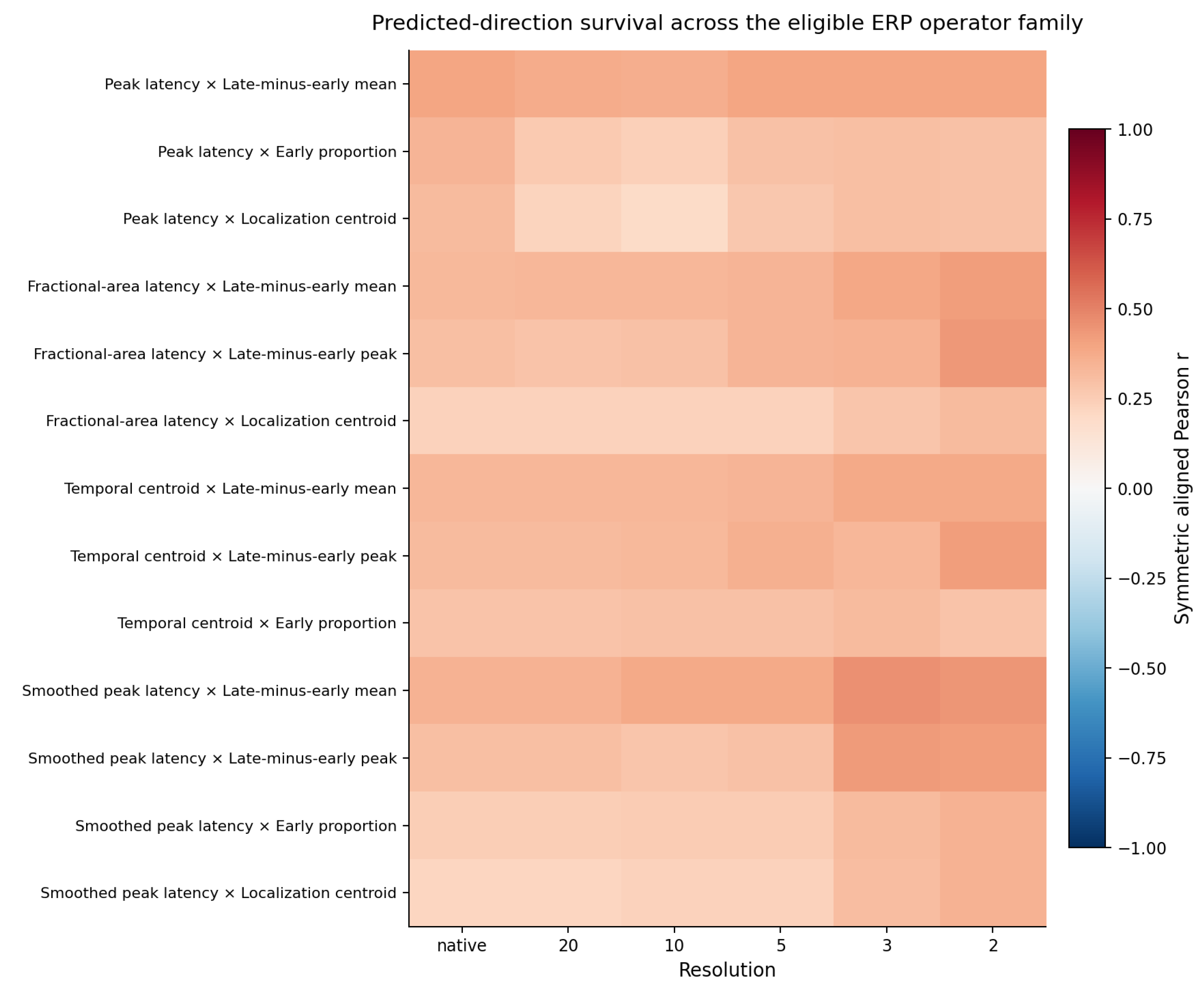
Appendix D.15. Post-Diagnostic Tie Sensitivities

The following analyses were performed after the primary compression outcome was known. They are post-diagnostic sensitivities and are not part of the frozen inferential layer.

One rectified participant profile, sub-040, was flat within the native timing interval in both halves.

Under the inherited native rule, the first maximal sample was returned:

$$300.78125\mathrm{ms}.$$

Under the finite-bin tie rule, the mean of tied bin centers was returned:

$$400\mathrm{ms}.$$

Two sensitivities were performed.

Appendix D.15.1. Participant Exclusion

Excluding sub-040 produced:

$$\Delta z=.0098,$$

with interval

$$[-.1457,.1881]$$

and

$$p=.448.$$

Appendix D.15.2. Mean Native Tie Location

Assigning the native flat profile the mean location of all tied native samples produced:

$$\Delta z=.0096,$$

with interval

$$[-.1396,.1828]$$

and

$$p=.446.$$

Both checks moved the point estimate slightly into the predicted direction. Neither produced a native-resolution advantage.

The unrectified analysis contained no native or compressed peak ties.

Table A43. Post-diagnostic tie sensitivities.

Analysis	$\Delta z$	95% interval	Predicted-direction p	Status
Exclude sub-040	.0098	[-.1457, .1881]	.448	Post-diagnostic
Mean native tied locations	.0096	[-.1396, .1828]	.446	Post-diagnostic

Table A43. Post-diagnostic tie sensitivities.

Analysis	$\Delta z$	95% interval	Predicted-direction p	Status
Exclude sub-040	.0098	[-.1457, .1881]	.448	Post-diagnostic
Mean native tied locations	.0096	[-.1396, .1828]	.446	Post-diagnostic

Appendix D.16. Frozen and Post-Diagnostic Layers

The compression evidence has three distinct status layers.

Appendix D.16.1. Frozen Prospective

• native-minus-three-bin rectified contrast;
• finite-resolution rectified trend;
• full rectified ladder;
• shared observer bootstrap;
• shared observer-pairing null;
• frozen tie rules;
• repeated-split extension.

Appendix D.16.2. Prospectively Specified Secondary

• unrectified native reconstruction;
• unrectified compression ladder;
• unrectified native-minus-three-bin contrast;
• rectified-minus-unrectified surface comparison;
• unrectified repeated splits.

Appendix D.16.3. Post-Diagnostic

• exclusion of sub-040;
• replacement of the native first-max tie with mean tied location.

The post-diagnostic checks clarify one operator edge case. They do not rescue, replace, or strengthen the frozen inference.

Appendix D.17. Protocol Conclusion

The prospective prediction was that native timing would support stronger observer recovery than a three-bin representation.

It did not.

The rectified focal contrast was effectively zero. The unrectified focal contrast was effectively zero. Both resolution ladders were positive and nonmonotonic. Repeated trial allocations supplied no native advantage. Alternative treatment of the one rectified flat profile did not change the result.

Three-bin compression removed most native peak-timing distinctions while preserving observer identity, broad temporal order, and the early–late localization axis.

Fine timing cardinality was not required for this observer relation.

The procedure counts and shared-mapping logic below follow the frozen analysis records and the declared shared-null framework. Dataset and artifact provenance remain documented separately.

Appendix E.1. General Correlation and Cross-Fit Statistic

For observer i, let $T_i^{\left(A\right)}$ denote timing estimated from data portion A, and let $L_i^{\left(B\right)}$ denote localization or allocation estimated from portion B.

The two directional correlations are

$$r_{A\to B}=corr\left({\left\{T_i^{\left(A\right)}\right\}}_{i=1}^N,{\left\{L_i^{\left(B\right)}\right\}}_{i=1}^N\right)$$

and

$$r_{B\to A}=corr\left({\left\{T_i^{\left(B\right)}\right\}}_{i=1}^N,{\left\{L_i^{\left(A\right)}\right\}}_{i=1}^N\right).$$

They are combined in Fisher space:

$$z_{\mathrm{sym}}={\displaystyle \frac{atanh\left(r_{A\to B}\right)+atanh\left(r_{B\to A}\right)}{2}},$$

with

$$r_{\mathrm{sym}}=tanh\left(z_{\mathrm{sym}}\right).$$

When an operator pair has a negative predicted direction, its raw correlation is multiplied by the frozen predicted sign before family aggregation. A positive aligned coefficient therefore supports the declared temporal relation.

Appendix E.2. Finite Permutation Probability

All permutation probabilities use the finite correction

$$p={\displaystyle \frac{b+1}{B+1}},$$

where:

• B is the number of valid permutation draws;
• b is the number of null statistics at least as extreme as the observed statistic in the declared direction.

The smallest reportable probability under 5,000 permutations is therefore

$${\displaystyle \frac{1}{5001}}\approx .0002.$$

No permutation probability is reported as zero.

Appendix E.3. ERP Participant Bootstrap

The primary ERP bootstrap estimates uncertainty in the symmetric observer-paired correlation across participants.

Appendix E.3.1. Statistic

$$r_{\mathrm{sym}}=tanh\left[{\displaystyle \frac{atanh\left(r_{A\to B}\right)+atanh\left(r_{B\to A}\right)}{2}}\right].$$

Appendix E.3.2. Resampling Unit

Participant.

Appendix E.3.3. Shared Mapping

One participant sample is used in both cross-fit directions within each draw.

For temporal-compression analyses, the same participant sample is also used across every resolution.

For rectified-versus-unrectified comparisons, the same inherited participant draw is used for both surfaces.

Appendix E.3.4. Seed and Iterations

• Seed: 2026071222
• Iterations: 2,000

Appendix E.3.5. Interval

Two-sided 95 percent percentile interval.

The 2.5th and 97.5th percentiles of the bootstrap statistic define the interval.

Appendix E.3.6. Preserved Structure

The procedure preserves:

• each participant’s paired timing and localization records;
• both directional estimates;
• the locked trial assignment;
• measurement-operator definitions;
• dependence among resolutions;
• dependence between rectified and unrectified surfaces where compared.

Appendix E.3.7. Resampled Structure

Participant membership in the analysis sample.

Appendix E.3.8. Licensed Inference

The bootstrap interval describes uncertainty in the declared observer-paired statistic under participant resampling.

It does not establish:

• independent replication;
• longitudinal stability;
• equivalence across measurement surfaces;
• independence of repeated trial splits.

Table A44. ERP participant-bootstrap procedures.

Analysis	Statistic	Shared structure	Seed	Draws	Interval
Primary ERP	Symmetric Fisher-z correlation	Both directions	2026071222	2,000	Two-sided percentile
Compression ladder	Recovery at each resolution	Directions and all resolutions	2026071222	2,000	Two-sided percentile
Native minus three bins	Paired $\Delta z$	Native and three-bin estimates	2026071222	2,000	Two-sided percentile
Unrectified ERP	Symmetric Fisher-z correlation	Both directions	2026071222	2,000	Two-sided percentile
Rectified minus unrectified	Paired surface difference	Both ERP surfaces	2026071222	2,000	Two-sided percentile

Table A44. ERP participant-bootstrap procedures.

Analysis	Statistic	Shared structure	Seed	Draws	Interval
Primary ERP	Symmetric Fisher-z correlation	Both directions	2026071222	2,000	Two-sided percentile
Compression ladder	Recovery at each resolution	Directions and all resolutions	2026071222	2,000	Two-sided percentile
Native minus three bins	Paired $\Delta z$	Native and three-bin estimates	2026071222	2,000	Two-sided percentile
Unrectified ERP	Symmetric Fisher-z correlation	Both directions	2026071222	2,000	Two-sided percentile
Rectified minus unrectified	Paired surface difference	Both ERP surfaces	2026071222	2,000	Two-sided percentile

Appendix E.4. ERP Observer-Pairing Permutation

The observer-pairing permutation tests whether timing and localization must belong to the same participant.

Appendix E.4.1. Statistic

The symmetric cross-fit Fisher-z statistic.

For the primary analysis:

$$S_{\mathrm{ERP}}=z_{\mathrm{sym}}.$$

For the compression experiment, the procedure also records:

$$\Delta z_{\mathrm{native}-3}=z_{\mathrm{native}}-z_{3-\mathrm{bin}}.$$

Appendix E.4.2. Resampling Unit

Participant identity on the localization side.

Appendix E.4.3. Shared Mapping

One permutation of the 40 participant labels is generated per iteration.

The same reassignment is used:

• in $A\to B$;
• in $B\to A$;
• across all temporal resolutions;
• across paired native-versus-compressed contrasts.

Appendix E.4.4. Seed and Iterations

• Seed: 2026071223
• Iterations: 5,000

Appendix E.4.5. Tail

For observer recovery:

$$H_A:z_{\mathrm{sym}}>0.$$

For the frozen compression contrast:

$$H_A:\Delta z_{\mathrm{native}-3}>0.$$

For the finite-resolution trend:

$$H_A:{\beta }_{{log}_{2}K}>0.$$

All are one-sided because their directions were declared prospectively.

Appendix E.4.6. Finite Correction

$$p={\displaystyle \frac{b+1}{5001}}.$$

Appendix E.4.7. Preserved Structure

The null preserves:

• every measured timing value;
• every measured localization value;
• marginal timing and localization distributions;
• participant sample size;
• trial split;
• operator definitions;
• both cross-fit directions;
• covariance among resolution conditions.

Appendix E.4.8. Broken Structure

The correct participant correspondence between timing and localization.

Appendix E.4.9. Licensed Inference

A small pairing probability establishes that correct participant identity carries more recovery than random reassignment of the same measured values.

It does not establish that:

• the relation is caused by one specific cognitive mechanism;
• every participant expresses the relation equally;
• the variables are independent of waveform morphology or signal quality.

Appendix E.5. ERP Repeated Trial Allocations

Repeated trial allocations test whether the observer relation depends on one convenient split of expected and unexpected trials.

Appendix E.5.1. Statistic

Symmetric cross-fit correlation at each declared resolution and ERP surface.

For compression stability, the paired statistic is

$$\Delta z_s=z_{\mathrm{native},s}-z_{3-\mathrm{bin},s}$$

for split s.

Appendix E.5.2. Resampling Unit

Trial assignment within participant and condition.

Appendix E.5.3. Shared Mapping

For each split:

• expected trials are reassigned to halves within participant;
• unexpected trials are reassigned separately;
• the same split is used for every operator and resolution evaluated in that repetition.

Appendix E.5.4. Seed and Iterations

• Starting seed: 2026071230
• Allocations: 200

The split index is incorporated into the deterministic seed sequence.

Appendix E.5.5. Tail

None.

Repeated splits are descriptive stability analyses rather than null-hypothesis tests.

Appendix E.5.6. Finite Correction

None.

Appendix E.5.7. Preserved Structure

The procedure preserves:

• the same 40 participants;
• the same eligible trial pool;
• 30 expected and 30 unexpected trials per half;
• operator definitions;
• analysis windows;
• participant identity.

Appendix E.5.8. Changed Structure

Which eligible trials enter half A and half B.

Appendix E.5.9. Licensed Inference

Repeated allocations show whether the result recurs across admissible trial partitions.

They do not provide:

• 200 independent replications;
• 200 independent participant samples;
• a larger effective sample size.

Appendix E.6. ERP Amplitude-Controlled Reduction

The amplitude-controlled analysis evaluates whether linear adjustment for half-specific response magnitude materially changes the point estimate.

Appendix E.6.1. Statistic

Directional correlations between residualized timing and localization, combined in Fisher space.

For $A\to B$:

• timing from half A is residualized against amplitude from half A;
• localization from half B is residualized against amplitude from half B.

The roles reverse for $B\to A$.

Appendix E.6.2. Resampling Unit

None in the reported manuscript reduction.

Appendix E.6.3. Shared Mapping

Not applicable.

Appendix E.6.4. Seed and Iterations

None.

Appendix E.6.5. Tail

None.

Appendix E.6.6. Finite Correction

None.

Appendix E.6.7. Preserved Structure

The procedure preserves:

• participant identity;
• trial split;
• timing and localization operators;
• both cross-fit directions.

Appendix E.6.8. Adjusted Structure

Linear association of each directional variable with its declared half-specific amplitude covariate.

Appendix E.6.9. Licensed Inference

The descriptive result shows that the point estimate is not absorbed by the declared linear amplitude terms.

It does not establish that every contribution of amplitude, signal quality, or waveform morphology has been removed.

Appendix E.7. Frozen Native-Versus-Three-Bin Contrast

The compression analysis tests the prospectively declared prediction that native peak timing should support stronger observer recovery than three-bin timing.

Appendix E.7.1. Statistic

$$\Delta z_{\mathrm{native}-3}=atanh\left(r_{\mathrm{native}}\right)-atanh\left(r_{3-\mathrm{bin}}\right).$$

Appendix E.7.2. Resampling Unit

Participant for the bootstrap; participant identity for the pairing permutation.

Appendix E.7.3. Shared Mapping

The same participant sample or reassignment is used:

• at native resolution;
• at three-bin resolution;
• in both cross-fit directions.

Appendix E.7.4. Seeds and Iterations

• Bootstrap: 2,000 draws, seed 2026071222
• Permutation: 5,000 draws, seed 2026071223

Appendix E.7.5. Tail

One-sided:

$$H_A:\Delta z_{\mathrm{native}-3}>0.$$

Appendix E.7.6. Finite Correction

For the permutation probability:

$$p={\displaystyle \frac{b+1}{5001}}.$$

Appendix E.7.7. Preserved Structure

The paired procedure preserves:

• participant identity within each resolution;
• dependence between native and compressed estimates;
• cross-fit directions;
• the same localization operator;
• the same trial split.

Appendix E.7.8. Compared Structure

Native peak-timing cardinality versus three ordered timing categories.

Appendix E.7.9. Licensed Inference

The procedure tests the frozen native-resolution advantage.

The observed interval and probability establish no detectable attenuation under the declared transformation and no evidence for the predicted advantage.

They do not establish statistical equivalence across resolutions.

Appendix E.8. Finite-Resolution Trend

The secondary frozen trend tests whether recovery increases systematically with the number of timing bins.

Appendix E.8.1. Statistic

For finite resolutions

$$K\in \{20,10,5,3,2\},$$

the analysis fits

$$z_K=\alpha +\beta {log}_{2}K+{\epsilon }_K.$$

The statistic is the slope

$$\beta .$$

Appendix E.8.2. Resampling Unit

Participant for bootstrap; participant identity for pairing permutation.

Appendix E.8.3. Shared Mapping

One participant draw or reassignment is shared across:

• every finite resolution;
• both cross-fit directions.

Appendix E.8.4. Seeds and Iterations

• Bootstrap: 2,000, seed 2026071222
• Permutation: 5,000, seed 2026071223

Appendix E.8.5. Tail

One-sided:

$$H_A:\beta >0.$$

Appendix E.8.6. Finite Correction

$$p={\displaystyle \frac{b+1}{5001}}.$$

Appendix E.8.7. Preserved Structure

The procedure preserves dependence among all resolution levels.

Appendix E.8.8. Tested Structure

Monotonic relation between timing cardinality and observer recovery.

Appendix E.8.9. Licensed Inference

The trend tests whether greater finite resolution systematically increases recovery.

It does not classify individual ladder rungs as independent experiments.

Appendix E.9. Rectified-Minus-Unrectified Paired Comparison

This comparison evaluates sensitivity of ERP recovery magnitude to zero rectification.

Appendix E.9.1. Statistic

At resolution K:

$$\Delta z_{\mathrm{rect}-\mathrm{unrect},K}=z_{\mathrm{rectified},K}-z_{\mathrm{unrectified},K}.$$

Appendix E.9.2. Resampling Unit

Participant.

Appendix E.9.3. Shared Mapping

The same participant bootstrap draw is used for:

• the rectified surface;
• the unrectified surface;
• both cross-fit directions;
• the same resolution.

Appendix E.9.4. Seed and Iterations

• Seed: 2026071222
• Iterations: 2,000

Appendix E.9.5. Tail

No directional hypothesis was declared.

The comparison uses a two-sided percentile interval.

Appendix E.9.6. Finite Correction

None.

Appendix E.9.7. Preserved Structure

The procedure preserves the paired participant data and all inherited analysis choices.

Appendix E.9.8. Changed Structure

Presence or absence of the zero floor after polarity orientation.

Appendix E.9.9. Licensed Inference

The paired interval describes the range of rectification-related differences compatible with participant resampling.

It does not establish equivalence between the surfaces.

The separate unrectified pairing test establishes whether recovery survives without rectification.

Appendix E.10. Natural Stories Family Statistic

For partition-specification unit j, let $z_j$ denote the symmetric, predicted-direction-aligned Fisher-z value.

The family statistic is

$$S_{\mathrm{family}}={median}_j{z}_j.$$

The reported family correlation is

$$r_{\mathrm{family}}=tanh\left(S_{\mathrm{family}}\right).$$

Predicted-direction preservation is

$$P_{\mathrm{sign}}=100\left({\displaystyle \frac{1}{J}}{\displaystyle \sum _{j=1}^J}\mathbf{1}[z_j>0]\right),$$

where J is the number of scored partition-specification estimates.

The locked clipped family contains:

$$J=125\times 10=\mathrm{1,250}.$$

The signed-safe family contains:

$$J=125\times 6=750.$$

The clipping-inactive diagnostic contains:

$$J=125\times 10=\mathrm{1,250}.$$

These values count dependent estimates. They are not independent sample sizes.

Appendix E.11. Natural Stories Shared Reader-Pairing Permutation

The reader-pairing null tests whether timing and localization or allocation must belong to the same reader.

Appendix E.11.1. Statistics

Two family statistics are evaluated:

1.

median symmetric predicted-direction-aligned Fisher z;

2.

predicted-direction preservation percentage.

Appendix E.11.2. Resampling Unit

Reader identity on the localization or allocation side.

Appendix E.11.3. Shared Mapping

For each iteration, one random key is generated for every reader in the starting universe.

The keys define one reader ordering.

That same ordering is:

• restricted to the common reader stratum;
• propagated across all scored partitions;
• used in both cross-fit directions;
• shared across raw and log reading time;
• shared across every operator pair.

For the clipping-inactive diagnostic, the global reader-key map is restricted separately to the 33-reader and 31-reader strata.

Appendix E.11.4. Seed and Iterations

For the dependence-preserving locked and secondary Natural Stories families:

• Seed: 2026071261
• Iterations: 5,000

Appendix E.11.5. Tails

For the family median:

$$H_A:S_{\mathrm{family},\mathrm{real}}>S_{\mathrm{family},\mathrm{null}}.$$

For sign preservation:

$$H_A:P_{\mathrm{sign},\mathrm{real}}>P_{\mathrm{sign},\mathrm{null}}.$$

Both are one-sided.

Appendix E.11.6. Finite Correction

$$p={\displaystyle \frac{b+1}{5001}}.$$

Appendix E.11.7. Preserved Structure

The permutation preserves:

• all reader timing values;
• all reader localization or allocation values;
• story partitions;
• reader strata;
• raw and log transforms;
• operator definitions;
• dependence among partition-specification estimates;
• both cross-fit directions.

Appendix E.11.8. Broken Structure

Correct correspondence between each reader’s timing and localization or allocation estimates.

Appendix E.11.9. Licensed Inference

A small family-level pairing probability establishes that the observed reader family exceeds families produced by random reassignment of the same measurements.

A small sign-preservation probability establishes that the consistency of the predicted direction exceeds the null distribution.

Neither probability turns the dependent partition-specification rows into independent observations.

Appendix E.12. Natural Stories Shared Reader Bootstrap

The reader bootstrap estimates uncertainty in the family median under resampling of readers.

Appendix E.12.1. Statistic

$$S_{\mathrm{family}}={median}_j{z}_j,$$

reported as

$$r_{\mathrm{family}}=tanh\left(S_{\mathrm{family}}\right).$$

Appendix E.12.2. Resampling Unit

Reader.

Appendix E.12.3. Shared Mapping

One reader-weight map is generated for the full starting reader universe and restricted to each active stratum.

For the secondary signed-safe and clipping-inactive analyses, bootstrap resampling is implemented through independent Poisson multiplicities:

$$w_i\sim Poisson\left(1\right).$$

Each reader is repeated according to $w_i$.

The same multiplicity map is propagated across:

• all partitions;
• both cross-fit directions;
• raw and log transforms;
• every operator pair;
• every active reader stratum.

The locked clipped analysis follows the same shared-reader principle over its 96-reader common stratum.

Appendix E.12.4. Seed and Iterations

• Seed: 2026071262
• Iterations: 2,000

Appendix E.12.5. Interval

Two-sided 95 percent percentile interval on the median Fisher-z, transformed back to correlation scale.

Appendix E.12.6. Tail

None.

The interval is not a directional hypothesis test.

Appendix E.12.7. Finite Correction

None.

Appendix E.12.8. Preserved Structure

The shared bootstrap preserves:

• the dependency among partitions;
• reuse of stories;
• reuse of operator components;
• both cross-fit directions;
• paired raw and log transforms;
• reader-stratum membership.

Appendix E.12.9. Resampled Structure

Reader contribution to the family statistic.

Appendix E.12.10. Licensed Inference

The interval describes reader-sampling uncertainty in the dependent family median.

It does not describe uncertainty from:

• sampling a new set of stories;
• selecting a new corpus;
• choosing a different operator family;
• treating 750 or 1,250 rows as independent observations.

Table A45. Natural Stories resampling procedures.

Family	Statistic	Reader stratum	Seed	Iterations	Output
Locked clipped	Median Fisher z; sign preservation	96	2026071261	5,000 permutations	Pairing and sign probabilities
Locked clipped	Median Fisher z	96	2026071262	2,000 bootstraps	95% interval
Signed-safe	Median Fisher z; sign preservation	96	2026071261	5,000 permutations	Pairing and sign probabilities
Signed-safe	Median Fisher z	96	2026071262	2,000 bootstraps	95% interval
Clipping-inactive	Median Fisher z; sign preservation	31–33	2026071261	5,000 permutations	Pairing and sign probabilities
Clipping-inactive	Median Fisher z	31–33	2026071262	2,000 bootstraps	95% interval

Table A45. Natural Stories resampling procedures.

Family	Statistic	Reader stratum	Seed	Iterations	Output
Locked clipped	Median Fisher z; sign preservation	96	2026071261	5,000 permutations	Pairing and sign probabilities
Locked clipped	Median Fisher z	96	2026071262	2,000 bootstraps	95% interval
Signed-safe	Median Fisher z; sign preservation	96	2026071261	5,000 permutations	Pairing and sign probabilities
Signed-safe	Median Fisher z	96	2026071262	2,000 bootstraps	95% interval
Clipping-inactive	Median Fisher z; sign preservation	31–33	2026071261	5,000 permutations	Pairing and sign probabilities
Clipping-inactive	Median Fisher z	31–33	2026071262	2,000 bootstraps	95% interval

Appendix E.13. Locked Clipped-Family Inference

Appendix E.13.1. Statistic

Median symmetric predicted-direction-aligned Fisher z across 1,250 dependent estimates.

Appendix E.13.2. Resampling Unit

Reader.

Appendix E.13.3. Shared Mapping

One reader reassignment or bootstrap sample across:

• 125 partitions;
• both directions;
• two reading-time transforms;
• five operator pairs.

Appendix E.13.4. Seeds and Iterations

• Permutation: 5,000, seed 2026071261
• Bootstrap: 2,000, seed 2026071262

Appendix E.13.5. Tails

One-sided for:

• family median;
• sign preservation.

Appendix E.13.6. Finite Correction

$$p={\displaystyle \frac{b+1}{5001}}.$$

Appendix E.13.7. Preserved Structure

The null preserves the clipped profiles, partitions, transforms, operators, and marginal reader values.

Appendix E.13.8. Broken Structure

Correct reader pairing.

Appendix E.13.9. Licensed Inference

The observed clipped family exceeds random reader reassignment.

The interval crossing zero shows that reader-sampling precision remains limited.

The positive pairing result and interval crossing zero answer different questions and are not contradictory.

Appendix E.14. Signed-Safe Family Inference

Appendix E.14.1. Statistic

Median symmetric predicted-direction-aligned Fisher z across 750 dependent estimates.

Appendix E.14.2. Resampling Unit

Reader.

Appendix E.14.3. Shared Mapping

One global reader-key or Poisson-weight map across:

• 125 partitions;
• both directions;
• raw and log reading time;
• three signed operator pairs.

Appendix E.14.4. Seeds and Iterations

• Permutation: 5,000, seed 2026071261
• Bootstrap: 2,000, seed 2026071262

Appendix E.14.5. Tails

One-sided for:

• median signed recovery;
• predicted-direction preservation.

Appendix E.14.6. Finite Correction

$$p={\displaystyle \frac{b+1}{5001}}.$$

Appendix E.14.7. Preserved Structure

The resampling preserves:

• the signed slope profiles;
• temporal direction;
• reader stratum;
• partition structure;
• operator-family dependence.

Appendix E.14.8. Broken Structure

Correct reader timing-to-allocation correspondence under permutation.

Appendix E.14.9. Licensed Inference

The procedure establishes strong signed reader-paired recovery above random reassignment and reader-sampling uncertainty.

It does not imply that the signed and clipped families are the same estimator.

Appendix E.15. Clipping-Inactive Diagnostic Inference

Appendix E.15.1. Statistic

Median symmetric predicted-direction-aligned Fisher z across 1,250 dependent estimates within selected clipping-inactive profiles.

Appendix E.15.2. Resampling Unit

Reader within the frozen selected strata.

Appendix E.15.3. Shared Mapping

One global reader-key or Poisson-weight map, restricted to:

• the 33-reader stratum;
• the 31-reader stratum.

The same map is shared across all partitions, directions, transforms, and operator pairs.

Appendix E.15.4. Seeds and Iterations

• Permutation: 5,000, seed 2026071261
• Bootstrap: 2,000, seed 2026071262

Appendix E.15.5. Tails

One-sided for:

• family median;
• sign preservation.

Appendix E.15.6. Finite Correction

$$p={\displaystyle \frac{b+1}{5001}}.$$

Appendix E.15.7. Preserved Structure

The procedure preserves:

• the original nonnegative operator family;
• profiles where clipping performed no transformation;
• selected reader strata;
• story and operator dependence.

Appendix E.15.8. Broken Structure

Correct reader correspondence under permutation.

Appendix E.15.9. Licensed Inference

The procedure establishes recurrence of the nonnegative reader relation where clipping was inactive.

It does not license population-wide generalization to the full 96-reader surface because profile inclusion depends on observed slope signs.

Appendix E.16. Clipping Audit

The clipping audit is deterministic.

Appendix E.16.1. Statistic

Counts and percentages of fully valid three-lag profiles with:

• zero clipped positions;
• one clipped position;
• two clipped positions;
• three clipped positions.

Appendix E.16.2. Resampling Unit

None.

Appendix E.16.3. Shared Mapping

None.

Appendix E.16.4. Seed and Iterations

None.

Appendix E.16.5. Tail

None.

Appendix E.16.6. Finite Correction

None.

Appendix E.16.7. Preserved Structure

All valid raw lag slopes and their reader, partition, side, lag, and transform identifiers.

Appendix E.16.8. Classified Structure

Whether each raw slope was below zero and therefore changed by the locked clipping rule.

Appendix E.16.9. Licensed Inference

The audit establishes how frequently clipping acted on the valid profile population.

It does not establish whether clipping caused, strengthened, or weakened reader-paired recovery. Those questions are addressed by the signed-safe and clipping-inactive analyses.

Appendix E.17. Pooling Diagnostics

Pooling is a deterministic transformation rather than a resampling procedure.

Appendix E.17.1. Statistic

The group-level waveform or lag profile after averaging across observers.

The observer relation is evaluated for definability rather than assigned a post-pooling correlation.

Appendix E.17.2. Resampling Unit

None.

Appendix E.17.3. Shared Mapping

None.

Appendix E.17.4. Seed and Iterations

None.

Appendix E.17.5. Tail

None.

Appendix E.17.6. Finite Correction

None.

Appendix E.17.7. Preserved Structure

Pooling preserves:

• the average ERP waveform or behavioral lag profile;
• the population-level condition contrast;
• broad temporal shape at the group level.

Appendix E.17.8. Broken Structure

Observer identity and the observer-indexed set of timing–localization pairs.

Appendix E.17.9. Licensed Inference

Pooling demonstrates whether the population effect survives aggregation and whether the observer relation remains estimable.

The relation is unavailable after pooling because its defining coordinate has been removed.

Appendix E.18. ERP Desynchronization Control

Desynchronization is a deterministic destructive transformation.

Appendix E.18.1. Statistic

Symmetric timing–localization recovery after the declared temporal displacement.

Family-level summaries include:

• median correlation;
• predicted-direction preservation.

Appendix E.18.2. Resampling Unit

None in the manuscript-grade diagnostic.

Appendix E.18.3. Shared Mapping

The same temporal shift is applied across the declared operator family.

Appendix E.18.4. Seed and Iterations

None.

Appendix E.18.5. Tail

None.

Appendix E.18.6. Finite Correction

None.

Appendix E.18.7. Preserved Structure

The control preserves:

• participant identity;
• trial assignment;
• amplitude values;
• operator family;
• sample size.

Appendix E.18.8. Broken Structure

The original temporal correspondence between timing and localization.

Appendix E.18.9. Licensed Inference

Auxiliary same-profile operator recovery collapsed under desynchronization, supporting the role of temporal alignment on the tested operator surface rather than marginal participant values alone.

Appendix E.19. ERP Temporal-Gradient Erasure

Gradient erasure is a deterministic destructive transformation.

Appendix E.19.1. Statistic

Median observer-paired correlation across the strict-window family before and after detrending.

Appendix E.19.2. Resampling Unit

None in the manuscript-grade diagnostic.

Appendix E.19.3. Shared Mapping

The same detrending operation is applied within each participant profile and declared window.

Appendix E.19.4. Seed and Iterations

None.

Appendix E.19.5. Tail

None.

Appendix E.19.6. Finite Correction

None.

Appendix E.19.7. Preserved Structure

The transformation preserves:

• participant identity;
• trial split;
• analysis window;
• residual profile variation;
• much of the original amplitude scale.

Appendix E.19.8. Broken Structure

First-order early-to-late temporal gradient.

Appendix E.19.9. Licensed Inference

Collapse after gradient erasure shows that first-order temporal organization carries the relation.

It does not identify the gradient as the only possible temporal carrier.

Appendix E.20. Post-Diagnostic Tie Sensitivities

The two tie analyses were performed after the frozen compression result was known.

Appendix E.20.1. Statistics

Native-minus-three-bin Fisher-z contrast after:

1.

excluding the participant with a flat native profile;

2.

replacing the inherited first-maximum native latency with the mean location of tied samples.

Appendix E.20.2. Resampling Unit

Participant.

Appendix E.20.3. Shared Mapping

The inherited paired participant-bootstrap and compression mappings were retained.

Appendix E.20.4. Seed and Iterations

• Bootstrap seed: 2026071222
• Bootstrap draws: 2,000
• Permutation seed: 2026071223
• Permutation draws: 5,000

Appendix E.20.5. Tail

One-sided in the inherited native-greater direction.

Appendix E.20.6. Finite Correction

$$p={\displaystyle \frac{b+1}{5001}}.$$

Appendix E.20.7. Preserved Structure

All frozen analysis choices except the declared tie treatment.

Appendix E.20.8. Changed Structure

Handling of one flat rectified participant profile.

Appendix E.20.9. Licensed Inference

These checks establish that the frozen result is not carried by the inherited treatment of that tie.

They do not acquire prospective status and do not alter the primary inferential layer.

Appendix E.21. Summary of Licensed Inference

Table A46. Nulls, controls, and the claims they license.

Procedure	Structure broken or resampled	Licensed inference
ERP participant bootstrap	Participant membership	Participant-sampling uncertainty
ERP pairing permutation	Correct participant correspondence	Recovery requires observer identity
ERP repeated splits	Trial-to-half assignment	Stability across trial partitions
Amplitude reduction	Linear amplitude association	Point estimate is not absorbed by declared amplitude terms
Compression contrast	Native timing cardinality	Test of frozen native-resolution advantage
Resolution trend	Number of finite timing bins	Test of monotonic resolution benefit
Rectified-minus-unrectified bootstrap	Zero rectification	Magnitude sensitivity across paired ERP surfaces
SPR reader permutation	Correct reader correspondence	Family recovery requires reader identity
SPR reader bootstrap	Reader contribution	Reader-sampling uncertainty in the family median
Clipping audit	None; deterministic classification	Prevalence of clipping
No-clipping diagnostic	Active clipping	Recurrence where clipping is inactive
Pooling	Observer identity	Group effect can survive while relation becomes unavailable
Desynchronization	Temporal correspondence	Same-profile operator recovery depends on alignment
Gradient erasure	First-order temporal shape	Same-profile operator recovery depends on temporal organization
Tie sensitivities	One tie-handling rule	Frozen result is not carried by the tie

Table A46. Nulls, controls, and the claims they license.

Procedure	Structure broken or resampled	Licensed inference
ERP participant bootstrap	Participant membership	Participant-sampling uncertainty
ERP pairing permutation	Correct participant correspondence	Recovery requires observer identity
ERP repeated splits	Trial-to-half assignment	Stability across trial partitions
Amplitude reduction	Linear amplitude association	Point estimate is not absorbed by declared amplitude terms
Compression contrast	Native timing cardinality	Test of frozen native-resolution advantage
Resolution trend	Number of finite timing bins	Test of monotonic resolution benefit
Rectified-minus-unrectified bootstrap	Zero rectification	Magnitude sensitivity across paired ERP surfaces
SPR reader permutation	Correct reader correspondence	Family recovery requires reader identity
SPR reader bootstrap	Reader contribution	Reader-sampling uncertainty in the family median
Clipping audit	None; deterministic classification	Prevalence of clipping
No-clipping diagnostic	Active clipping	Recurrence where clipping is inactive
Pooling	Observer identity	Group effect can survive while relation becomes unavailable
Desynchronization	Temporal correspondence	Same-profile operator recovery depends on alignment
Gradient erasure	First-order temporal shape	Same-profile operator recovery depends on temporal organization
Tie sensitivities	One tie-handling rule	Frozen result is not carried by the tie

Appendix E.22. Appendix Summary

The inferential architecture preserves dependence rather than pretending it is absent.

ERP bootstraps resample participants while sharing the draw across directions, resolutions, and paired surfaces. ERP pairing nulls share one reassignment across those same dependent quantities. Repeated trial allocations change the split while retaining the same participants and trial pool.

Natural Stories permutations and bootstraps share one reader mapping across partitions, directions, transforms, operator pairs, and reader strata. Family statistics summarize dependent estimates rather than treating them as independent observations.

Pooling, desynchronization, gradient erasure, and clipping audits are deterministic transformations. Their role is structural: they identify which coordinate has been preserved or removed.

The nulls and resampling procedures therefore answer distinct questions:

• Does the relation require correct observer identity?
• How uncertain is the relation under observer resampling?
• Does it recur across alternative trial allocations?
• Does severe compression attenuate it?
• Does rectification create it?
• Does clipping create it?
• Which temporal transformations destroy it?

The procedures are aligned to those questions and license no broader inference than the coordinate each one tests.

Appendix F.1. ERP Directional Results

The primary ERP relation was positive in both cross-fit directions.

Table A47. Native ERP directional results.

Surface and statistic	$A\to B$	$B\to A$	Symmetric
Rectified Pearson	.442	.343	.393
Rectified Spearman	.458	.367	.413
Rectified amplitude controlled	.449	.413	.431
Unrectified Pearson	.428	.223	.330
Unrectified Spearman	.426	.225	.329
Unrectified amplitude controlled	.426	.373	.400

Table A47. Native ERP directional results.

Surface and statistic	$A\to B$	$B\to A$	Symmetric
Rectified Pearson	.442	.343	.393
Rectified Spearman	.458	.367	.413
Rectified amplitude controlled	.449	.413	.431
Unrectified Pearson	.428	.223	.330
Unrectified Spearman	.426	.225	.329
Unrectified amplitude controlled	.426	.373	.400

The weaker unrectified $B\to A$ coefficient reduced the symmetric point estimate relative to the rectified surface, but both directions remained positive. The relation therefore did not depend on one favorable direction or on zero rectification.

Appendix F.2. Unrectified ERP Directions Across Temporal Resolution

The unrectified sensitivity retained positive directional and symmetric recovery across the full inherited resolution ladder.

Table A48. Directional unrectified ERP results across resolution.

Resolution	$A\to B$	$B\to A$	Symmetric r	Symmetric Spearman $\rho$	Descriptive amplitude-controlled r
Native	.428	.223	.330	.329	.400
20 bins	.437	.202	.325	.361	.342
10 bins	.404	.224	.317	.325	.340
5 bins	.451	.326	.390	.387	.447
3 bins	.326	.340	.333	.315	.401
2 bins	.393	.332	.363	.348	.397

Table A48. Directional unrectified ERP results across resolution.

Resolution	$A\to B$	$B\to A$	Symmetric r	Symmetric Spearman $\rho$	Descriptive amplitude-controlled r
Native	.428	.223	.330	.329	.400
20 bins	.437	.202	.325	.361	.342
10 bins	.404	.224	.317	.325	.340
5 bins	.451	.326	.390	.387	.447
3 bins	.326	.340	.333	.315	.401
2 bins	.393	.332	.363	.348	.397

The three-bin result is especially informative. The two directions were nearly identical:

$$r_{A\to B}=.326,r_{B\to A}=.340,$$

producing

$$r_{\mathrm{sym}}=.333.$$

Three-bin preservation was therefore not produced by one cross-fit direction compensating for the failure of the other.

Appendix F.3. Natural Stories Partition and Reader Registry

The locked clipped and signed-safe families used the same 125 scored partitions:

$$\mathrm{P}002\mathrm{through}\mathrm{P}126.$$

Each used a common stratum of 96 readers.

The clipping-inactive diagnostic used the same scored partition range but divided it into two reader strata:

• P002 through P056: 55 partitions, 33 readers;
• P057 through P126: 70 partitions, 31 readers.

P001 remained unscored in every behavioral family because its common-reader count fell below the declared minimum of 30.

Table A49. Behavioral partition and reader structure.

Surface	Partition identifiers	Scored partitions	Common readers	Stratum
Locked clipped concentration	P002–P126	125	96	S001
Signed temporal allocation	P002–P126	125	96	S001
Clipping-inactive concentration	P002–P056	55	33	S001
Clipping-inactive concentration	P057–P126	70	31	S002

Table A49. Behavioral partition and reader structure.

Surface	Partition identifiers	Scored partitions	Common readers	Stratum
Locked clipped concentration	P002–P126	125	96	S001
Signed temporal allocation	P002–P126	125	96	S001
Clipping-inactive concentration	P002–P056	55	33	S001
Clipping-inactive concentration	P057–P126	70	31	S002

Partition identity and reader count must appear on every row of the released direction-level output. They cannot be inferred only from row order.

Appendix F.4. Locked Clipped Specification-Level Results

Table F4 reports medians across the 125 scored partitions for each locked behavioral specification.

The two directional columns contain raw correlation medians. The symmetric column is predicted-sign aligned. For specifications with a negative predicted direction, the raw negative relation becomes positive after alignment.

The decomposition explains the locked family result. The strongest specifications concern temporal location. Peak lag relates strongly to current-token concentration and late-minus-early cost under both reading-time transforms. General concentration pairs are much weaker.

The locked median of $r=.103$ therefore combines two distinct patterns:

• strong location-sensitive relations;
• weak general concentration relations.

That heterogeneity motivated the signed-safe operator family.

Table A50. Locked clipped concentration results by specification.

RT	Timing operator	Localization operator	Predicted sign	Median $A\to B$	Median $B\to A$	Median symmetric signed r	Positive partitions
Log	Spillover ratio	Cost concentration	(-)	-.012	-.121	.073	114/125
Log	Lag-weighted allocation	Cost concentration	(-)	.029	-.067	.021	79/125
Log	Peak lag	Cost concentration	(-)	.009	-.055	.020	95/125
Log	Peak lag	Current-token concentration	(-)	-.522	-.469	.497	125/125
Log	Peak lag	Late-minus-early cost	(+)	.467	.452	.461	125/125
Raw	Spillover ratio	Cost concentration	(-)	-.046	-.160	.099	125/125
Raw	Lag-weighted allocation	Cost concentration	(-)	-.018	-.097	.058	111/125
Raw	Peak lag	Cost concentration	(-)	-.018	-.038	.025	87/125
Raw	Peak lag	Current-token concentration	(-)	-.447	-.450	.452	125/125
Raw	Peak lag	Late-minus-early cost	(+)	.414	.416	.416	125/125

Table A50. Locked clipped concentration results by specification.

RT	Timing operator	Localization operator	Predicted sign	Median $A\to B$	Median $B\to A$	Median symmetric signed r	Positive partitions
Log	Spillover ratio	Cost concentration	(-)	-.012	-.121	.073	114/125
Log	Lag-weighted allocation	Cost concentration	(-)	.029	-.067	.021	79/125
Log	Peak lag	Cost concentration	(-)	.009	-.055	.020	95/125
Log	Peak lag	Current-token concentration	(-)	-.522	-.469	.497	125/125
Log	Peak lag	Late-minus-early cost	(+)	.467	.452	.461	125/125
Raw	Spillover ratio	Cost concentration	(-)	-.046	-.160	.099	125/125
Raw	Lag-weighted allocation	Cost concentration	(-)	-.018	-.097	.058	111/125
Raw	Peak lag	Cost concentration	(-)	-.018	-.038	.025	87/125
Raw	Peak lag	Current-token concentration	(-)	-.447	-.450	.452	125/125
Raw	Peak lag	Late-minus-early cost	(+)	.414	.416	.416	125/125

Appendix F.5. Signed-Safe Specification-Level Results

Every signed-safe specification was positive in both directional medians and across all 125 scored partitions.

Table A51. Signed temporal-allocation results by specification.

RT	Timing operator	Allocation operator	Median $A\to B$	Median $B\to A$	Median symmetric r	Positive partitions
Log	Signed lag trend	Signed late-minus-early allocation	.722	.721	.709	125/125
Log	Signed peak lag	Signed endpoint contrast	.508	.501	.508	125/125
Log	Signed peak lag	Signed late-minus-early allocation	.460	.448	.454	125/125
Raw	Signed lag trend	Signed late-minus-early allocation	.685	.674	.678	125/125
Raw	Signed peak lag	Signed endpoint contrast	.452	.453	.454	125/125
Raw	Signed peak lag	Signed late-minus-early allocation	.417	.413	.415	125/125

Table A51. Signed temporal-allocation results by specification.

RT	Timing operator	Allocation operator	Median $A\to B$	Median $B\to A$	Median symmetric r	Positive partitions
Log	Signed lag trend	Signed late-minus-early allocation	.722	.721	.709	125/125
Log	Signed peak lag	Signed endpoint contrast	.508	.501	.508	125/125
Log	Signed peak lag	Signed late-minus-early allocation	.460	.448	.454	125/125
Raw	Signed lag trend	Signed late-minus-early allocation	.685	.674	.678	125/125
Raw	Signed peak lag	Signed endpoint contrast	.452	.453	.454	125/125
Raw	Signed peak lag	Signed late-minus-early allocation	.417	.413	.415	125/125

The two strongest specifications used signed lag trend rather than peak lag:

$$r=.709$$

under log reading time and

$$r=.678$$

under raw reading time.

This consistency shows that the family-level result is not a peak-estimator artifact. Continuous signed lag change carries even stronger reader organization than the discrete peak-position operators.

Appendix F.6. Clipping-Inactive Specification-Level Results

The clipping-inactive diagnostic retained the original nonnegative formulas while restricting the analysis to profiles on which clipping changed nothing.

Directional medians are reported on the raw correlation scale. Symmetric values are aligned to the predicted direction.

Table A52. Clipping-inactive concentration results by specification.

RT	Timing operator	Localization operator	Predicted sign	Median $A\to B$	Median $B\to A$	Median symmetric signed r	Positive partitions
Log	Spillover ratio	Cost concentration	(-)	-.112	-.055	.101	103/125
Log	Lag-weighted allocation	Cost concentration	(-)	-.137	-.124	.133	119/125
Log	Peak lag	Cost concentration	(-)	-.107	-.231	.202	112/125
Log	Peak lag	Current-token concentration	(-)	-.317	-.347	.356	125/125
Log	Peak lag	Late-minus-early cost	(+)	.271	.280	.271	125/125
Raw	Spillover ratio	Cost concentration	(-)	-.197	-.099	.162	119/125
Raw	Lag-weighted allocation	Cost concentration	(-)	-.191	-.078	.131	118/125
Raw	Peak lag	Cost concentration	(-)	-.151	-.073	.124	109/125
Raw	Peak lag	Current-token concentration	(-)	-.305	-.319	.338	123/125
Raw	Peak lag	Late-minus-early cost	(+)	.312	.317	.312	125/125

Table A52. Clipping-inactive concentration results by specification.

RT	Timing operator	Localization operator	Predicted sign	Median $A\to B$	Median $B\to A$	Median symmetric signed r	Positive partitions
Log	Spillover ratio	Cost concentration	(-)	-.112	-.055	.101	103/125
Log	Lag-weighted allocation	Cost concentration	(-)	-.137	-.124	.133	119/125
Log	Peak lag	Cost concentration	(-)	-.107	-.231	.202	112/125
Log	Peak lag	Current-token concentration	(-)	-.317	-.347	.356	125/125
Log	Peak lag	Late-minus-early cost	(+)	.271	.280	.271	125/125
Raw	Spillover ratio	Cost concentration	(-)	-.197	-.099	.162	119/125
Raw	Lag-weighted allocation	Cost concentration	(-)	-.191	-.078	.131	118/125
Raw	Peak lag	Cost concentration	(-)	-.151	-.073	.124	109/125
Raw	Peak lag	Current-token concentration	(-)	-.305	-.319	.338	123/125
Raw	Peak lag	Late-minus-early cost	(+)	.312	.317	.312	125/125

The selected-profile family reproduces the same broad decomposition seen in the locked surface. Peak lag paired with current-token concentration or late-minus-early cost remains stronger than the general cost-concentration pairs.

Clipping therefore does not create the location-sensitive pattern.

Appendix F.7. Partition-Level Directional Results

Each scored behavioral row must identify:

• analysis surface;
• stratum;
• partition;
• reader count;
• reading-time transform;
• timing operator;
• localization or allocation operator;
• predicted sign;
• $A\to B$ raw correlation;
• $B\to A$ raw correlation;
• predicted-sign-aligned directional correlations;
• symmetric Fisher z;
• symmetric signed correlation.

The complete table is too large for a paper-facing appendix:

• locked clipped family: 1,250 rows;
• signed-safe family: 750 rows;
• clipping-inactive family: 1,250 rows.

The v1.1 package records the corresponding partition-level directional and specification fields in:

• outputs/spr/sprcrossfitdirectionalstatistics.csv;
• outputs/spr/sprcrossfitpartitionspecificationstatistics.csv.

The v1.1 SPR exports contain directional coefficients and specification identifiers in the partition-level records.

Table A53. Example partition-level direction records.

Surface	Partition	Readers	RT	Operator pair	$A\to B$	$B\to A$	Symmetric signed r
Clipped concentration	P002	96	Log	Peak lag × current-token concentration	-.454	-.366	.411
Signed allocation	P002	96	Log	Signed lag trend × signed late-minus-early allocation	.538	.504	.521
Clipping-inactive concentration	P002	33	Log	Peak lag × current-token concentration	-.191	-.298	.245
Signed allocation	P064	96	Log	Signed lag trend × signed late-minus-early allocation	.552	.647	.602
Clipping-inactive concentration	P064	31	Raw	Peak lag × current-token concentration	-.368	-.305	.337
Signed allocation	P126	96	Raw	Signed peak lag × signed endpoint contrast	.398	.368	.383

Table A53. Example partition-level direction records.

Surface	Partition	Readers	RT	Operator pair	$A\to B$	$B\to A$	Symmetric signed r
Clipped concentration	P002	96	Log	Peak lag × current-token concentration	-.454	-.366	.411
Signed allocation	P002	96	Log	Signed lag trend × signed late-minus-early allocation	.538	.504	.521
Clipping-inactive concentration	P002	33	Log	Peak lag × current-token concentration	-.191	-.298	.245
Signed allocation	P064	96	Log	Signed lag trend × signed late-minus-early allocation	.552	.647	.602
Clipping-inactive concentration	P064	31	Raw	Peak lag × current-token concentration	-.368	-.305	.337
Signed allocation	P126	96	Raw	Signed peak lag × signed endpoint contrast	.398	.368	.383

The excerpt is illustrative only. Family inference is calculated from the full registered surface, not from selected partitions.

Appendix F.8. Partition-Level Coefficient Construction

For partition p, specification s, and direction d, let

$$r_{psd}$$

denote the raw reader-paired coefficient.

Let

$$q_s\in \{-1,+1\}$$

denote the declared predicted sign.

The aligned directional coefficient is

$${\tilde{r}}_{psd}=q_s{r}_{psd}.$$

The symmetric Fisher value is

$$z_{ps}={\displaystyle \frac{atanh\left({\tilde{r}}_{ps,A\to B}\right)+atanh\left({\tilde{r}}_{ps,B\to A}\right)}{2}}.$$

The symmetric signed correlation is

$${\tilde{r}}_{ps}=tanh\left(z_{ps}\right).$$

This construction preserves the two directional coefficients in the released record. The family summary does not replace or erase them.

Appendix F.9. Directional Asymmetry

Directional differences occur in both ERP and Natural Stories.

In ERP, the primary rectified relation was stronger for $A\to B$ than for $B\to A$:

$$.442\mathrm{versus}.343.$$

The unrectified difference was larger:

$$.428\mathrm{versus}.223.$$

In the signed Natural Stories family, the direction medians were closely matched within every specification. For example, the strongest log specification produced:

$$.722\mathrm{and}.721.$$

This directional balance contributed to the strength of the signed family.

The clipped concentration family was more asymmetric. Several weak cost-concentration specifications produced one directional median near zero and a stronger coefficient in the other direction. The stronger location-sensitive pairs were more balanced.

Directional asymmetry is therefore part of the operator result. The symmetric statistic prevents either arbitrary half or partition side from defining the final estimate, while the directional record shows where instability remains.

Appendix F.10. Family Summaries

Table A54. ERP and Natural Stories family summaries.

Analysis	Observers	Partitions or splits	Specifications	Symmetric or family r	Interval	Pairing p	Direction preservation
Rectified ERP primary	40	Locked split	1 canonical pair	.393	[.207, .554]	.0004	Both directions positive
Unrectified ERP	40	Locked split	1 canonical pair	.330	[.060, .561]	.0026	Both directions positive
Rectified ERP repeated splits	40	200	1 canonical pair	Median .305	IQR [.256, .361]	Not assigned	200/200 positive
Unrectified ERP repeated splits	40	200	1 canonical pair	Median .332	IQR [.269, .390]	Not assigned	200/200 positive
Clipped concentration SPR	96	125	10	.103	[-.026, .297]	.0162	88.88%
Signed allocation SPR	96	125	6	.491	[.407, .577]	.0002	100%
Clipping-inactive SPR	31–33	125	10	.206	[.044, .363]	.0002	94.24%

Table A54. ERP and Natural Stories family summaries.

Analysis	Observers	Partitions or splits	Specifications	Symmetric or family r	Interval	Pairing p	Direction preservation
Rectified ERP primary	40	Locked split	1 canonical pair	.393	[.207, .554]	.0004	Both directions positive
Unrectified ERP	40	Locked split	1 canonical pair	.330	[.060, .561]	.0026	Both directions positive
Rectified ERP repeated splits	40	200	1 canonical pair	Median .305	IQR [.256, .361]	Not assigned	200/200 positive
Unrectified ERP repeated splits	40	200	1 canonical pair	Median .332	IQR [.269, .390]	Not assigned	200/200 positive
Clipped concentration SPR	96	125	10	.103	[-.026, .297]	.0162	88.88%
Signed allocation SPR	96	125	6	.491	[.407, .577]	.0002	100%
Clipping-inactive SPR	31–33	125	10	.206	[.044, .363]	.0002	94.24%

Appendix F.11. Release-Table Schema

The machine-readable SPR direction tables use the following column order:

1.

analysis;

2.

scientific_status;

3.

stratum_id;

4.

partition_id;

5.

common_reader_n;

6.

rt_transform;

7.

spec_id;

8.

timing_metric;

9.

localization_metric;

10.

predicted_sign;

11.

a_to_b_raw_r;

12.

b_to_a_raw_r;

13.

a_to_b_signed_r;

14.

b_to_a_signed_r;

15.

symmetric_fisher_z;

16.

symmetric_signed_r;

17.

sign_preserved;

18.

source_registry;

19.

source_notebook;

20.

release_version.

The row order is explicit and reproducible. No result depends on an undocumented assumption that every group of six or ten rows corresponds to one partition.

Appendix F.12. Appendix Summary

The directional record supports the family-level conclusions.

The ERP relation is positive in both cross-fit directions on rectified and unrectified surfaces. Three-bin unrectified recovery is also balanced across directions.

The locked Natural Stories family is heterogeneous. Its strongest relations involve temporal location, while general concentration pairs are smaller and more directionally uneven.

The signed-safe family is strong in every specification and balanced across directions. Every partition supports the predicted direction.

The clipping-inactive diagnostic recovers the original nonnegative relation in smaller selected reader strata, with the strongest effects again appearing in location-sensitive pairs.

The family summaries therefore compress a real and interpretable specification structure. Signed temporal allocation carries the broadest and strongest behavioral recovery.

Appendix G.1. Diagnostic Preservation Map

Table A55. Auxiliary transformations and their evidentiary roles.

Diagnostic	Transformation	Preserved coordinates	Removed coordinates	Result	Evidentiary role
Pooling	Average profiles across observers before constructing observer metrics	Group condition effect; gross temporal surface	Observer identity; between-observer pairing	Canonical group effect preserved; observer relation unavailable	Estimand demonstration
Observer reassignment	Permute localization or allocation identities while retaining measured values	Marginal values; operators; split or partition structure	Correct observer correspondence	ERP and behavioral recovery exceed reassigned pairing	Identity test; primary inference specified in Appendix E
Desynchronization	Shift timing and localization operators out of their declared temporal correspondence	Observer identity; signal values; sample size	Temporal alignment	ERP formula-distinct family median falls from approximately .620 to .005; sign preservation falls to approximately 31.9%	Destructive alignment diagnostic
Gradient erasure	Remove first-order temporal trend within the declared ERP window	Observer identity; residual waveform variation; analysis window	Early-to-late gradient structure	Strict-window median falls from approximately .638 to .010	Destructive shape diagnostic
Speed control	Residualize behavioral timing and localization against global reader speed	Reader identity; temporal profile; operator pairing	Linear global-speed component	No observer-separated coefficient assigned; retained as an alternative-mechanism design check	Defined alternative-mechanism check
Total-cost control	Add gross processing cost to the behavioral residualization	Reader identity; lag organization; pairing	Linear speed and total-cost components	No observer-separated coefficient assigned; retained as a magnitude-reduction design check	Defined magnitude-reduction check
Same-profile geometry	Compare observed operator-family structure with geometry-preserving synthesis or reassignment models	One-profile operator geometry; declared admissibility	Selected identity, residual, direction, or concentration correspondence	ERP exceeds its conditioned residual null; SPR lies in the upper tail of its declared geometry null but remains nondecisive	Supporting geometry diagnostic

Table A55. Auxiliary transformations and their evidentiary roles.

Diagnostic	Transformation	Preserved coordinates	Removed coordinates	Result	Evidentiary role
Pooling	Average profiles across observers before constructing observer metrics	Group condition effect; gross temporal surface	Observer identity; between-observer pairing	Canonical group effect preserved; observer relation unavailable	Estimand demonstration
Observer reassignment	Permute localization or allocation identities while retaining measured values	Marginal values; operators; split or partition structure	Correct observer correspondence	ERP and behavioral recovery exceed reassigned pairing	Identity test; primary inference specified in Appendix E
Desynchronization	Shift timing and localization operators out of their declared temporal correspondence	Observer identity; signal values; sample size	Temporal alignment	ERP formula-distinct family median falls from approximately .620 to .005; sign preservation falls to approximately 31.9%	Destructive alignment diagnostic
Gradient erasure	Remove first-order temporal trend within the declared ERP window	Observer identity; residual waveform variation; analysis window	Early-to-late gradient structure	Strict-window median falls from approximately .638 to .010	Destructive shape diagnostic
Speed control	Residualize behavioral timing and localization against global reader speed	Reader identity; temporal profile; operator pairing	Linear global-speed component	No observer-separated coefficient assigned; retained as an alternative-mechanism design check	Defined alternative-mechanism check
Total-cost control	Add gross processing cost to the behavioral residualization	Reader identity; lag organization; pairing	Linear speed and total-cost components	No observer-separated coefficient assigned; retained as a magnitude-reduction design check	Defined magnitude-reduction check
Same-profile geometry	Compare observed operator-family structure with geometry-preserving synthesis or reassignment models	One-profile operator geometry; declared admissibility	Selected identity, residual, direction, or concentration correspondence	ERP exceeds its conditioned residual null; SPR lies in the upper tail of its declared geometry null but remains nondecisive	Supporting geometry diagnostic

Appendix G.2. Pooling

Pooling asks whether the observer relation remains measurable after participant or reader profiles are averaged.

It does not.

For ERP, pooling retains a recognizable semantic-negativity waveform and the canonical population contrast. Timing and early–late localization can still be described for that one pooled waveform. There is no longer a collection of participant-indexed timing and localization pairs across which covariance can be estimated.

For Natural Stories, pooling likewise retains a gross current-to-spillover processing-cost profile. It removes the reader axis required to ask whether one reader’s timing corresponds to that reader’s allocation.

The result is therefore structural:

$${{\mathcal{S}}_i}_{i=1}^N⟶\overline{\mathcal{S}}$$

replaces an indexed family with one aggregate surface. The observer relation becomes unavailable because its defining coordinate has been removed.

Pooling does not supply an independent test of the access interpretation. It demonstrates why a canonical group effect and an unmeasured observer relation can coexist.

Table A56. Pooling diagnostics.

Surface	Population object after pooling	Observer relation after pooling
ERP	Gross semantic-negativity contrast preserved	Undefined
Natural Stories	Gross lagged cost profile preserved	Undefined

Table A56. Pooling diagnostics.

Surface	Population object after pooling	Observer relation after pooling
ERP	Gross semantic-negativity contrast preserved	Undefined
Natural Stories	Gross lagged cost profile preserved	Undefined

Appendix G.3. Observer Reassignment

Observer reassignment preserves the measured timing and localization values while breaking the identity mapping between them.

For ERP, one permutation of participant identity was shared across both cross-fit directions. Correct pairing produced

$$r=.393$$

with a finite observer-pairing probability of

$$p=.0004.$$

For the locked clipped Natural Stories family, correct reader pairing exceeded the shared reassignment family with

$$p=.0162.$$

The signed-safe family produced

$$p=.0002,$$

and the clipping-inactive diagnostic also produced

$$p=.0002.$$

The procedures differ in their measurement surfaces, but their interpretation is the same. The relation is carried by the correspondence between independently constructed quantities belonging to the same observer. It is not recoverable from the marginal distributions alone.

Observer reassignment does not identify the cognitive source of the correspondence. Stable morphology, signal quality, processing traits, and observer-specific access organization remain possible contributors. It establishes that identity pairing is empirically consequential.

Appendix G.4. Desynchronization

The ERP desynchronization control shifts timing and localization operators out of their original temporal correspondence while retaining participants, waveforms, operator formulas, and sample size.

In the aligned same-profile operator family, the median Pearson relation was approximately

$$r=.620.$$

Under the declared $\pm 250$-ms displacement, the median fell to approximately

$$r=.005,$$

and predicted-direction preservation fell to approximately 31.9 percent.

The transformation attacks alignment rather than information quantity. The participant profiles remain available, and the values entering the operators are still drawn from the same waveforms. What changes is whether the timing and localization operators refer to corresponding temporal regions.

Auxiliary same-profile operator recovery collapsed under desynchronization, supporting the role of temporal alignment on the tested operator surface. It does not establish that temporal alignment uniquely reflects semantic access.

The manuscript-grade sources are:

• erp_desync_sweep.csv;
• erp_desync_perspec.csv.

Appendix G.5. Temporal-Gradient Erasure

The temporal-gradient control asks whether observer recovery survives removal of first-order early-to-late structure.

Within each participant profile, a linear temporal component was estimated and removed over the declared strict window. Participant identity, the analysis interval, residual waveform variation, and the operator family remained available.

Before erasure, the strict-window family median was approximately

$$r=.638.$$

After detrending, it was approximately

$$r=.010.$$

Auxiliary same-profile operator recovery collapsed when the first-order temporal gradient was removed.

This result supports the role of first-order temporal organization on the tested operator surface. Early-to-late waveform organization contributes directly to the same-profile relation.

The control does not identify the linear gradient as the unique carrier. Width, asymmetry, rank, and other correlated morphological properties may accompany it. Its evidentiary role is narrower: targeted removal of first-order temporal structure collapses auxiliary same-profile operator recovery.

The manuscript-grade source is:

erp_window_sensitivity.csv

The files

• erptemporalgradienterasure.csv;
• erptemporalgradienterasuresummary.csv

are auxiliary implementation records and do not independently carry the manuscript claim.

Appendix G.6. Global-Speed Control

Global reader speed is an obvious behavioral alternative. A reader who responds more slowly across the corpus could appear later on multiple temporal measures even when no profile-specific allocation relation exists.

The speed diagnostic residualizes the declared behavioral timing and localization quantities against a reader-level summary of overall reading speed. The relevant comparison is between the unadjusted relation and the relation among speed-residualized quantities.

The available speed-control partial correlations were calculated on a same-profile behavioral operator block containing algebraically coupled two-position specifications. They are not used as evidence for the observer-separated families. No speed-control coefficient is assigned to the signed-safe or clipping-inactive families, consistent with the decision to stop after the prospectively specified sensitivities.

The diagnostic therefore has a defined but bounded role:

• it identifies the general-speed reduction that an independent study should test;
• it preserves the historical analysis record in the release ledger;
• it does not supply a current numerical claim for the clipped, signed-safe, or clipping-inactive cross-fit families.

No statement in the main text depends on a speed-adjusted behavioral coefficient.

Appendix G.7. Total-Cost Control

Total processing cost is distinct from temporal allocation. Two readers can express similar cumulative surprisal-linked cost while distributing it differently across the current word and spillover positions.

The total-cost diagnostic extends the speed reduction by residualizing the timing and localization quantities against both:

1.

global reader speed;

2.

total lag-profile cost.

The speed-only partial correlations came from a same-profile construction and are not used as evidence for the observer-separated behavioral families. No observer-separated speed-control coefficient is assigned to the clipped, signed-safe, or clipping-inactive families.

The retained inference is conceptual and prospective. A future behavioral study should construct total cost and temporal allocation from prospectively balanced observations, then test whether allocation remains observer-paired after the magnitude term is removed.

No same-profile partial correlation is used to claim that total processing burden has been eliminated.

Table A57. Status of behavioral reduction controls.

Control	Alternative targeted	Current numerical status	Licensed use
Global speed	General faster-versus-slower reader organization	No observer-separated coefficient assigned	Defines a live reduction test
Speed plus total cost	General speed and gross processing burden	No observer-separated coefficient assigned	Separates allocation from magnitude prospectively

Table A57. Status of behavioral reduction controls.

Control	Alternative targeted	Current numerical status	Licensed use
Global speed	General faster-versus-slower reader organization	No observer-separated coefficient assigned	Defines a live reduction test
Speed plus total cost	General speed and gross processing burden	No observer-separated coefficient assigned	Separates allocation from magnitude prospectively

Appendix G.8. Same-Profile Geometry

Same-profile analyses examine timing and localization operators extracted from one waveform or lag profile. They are useful because they reveal which geometric relations are present on the measured surface. They cannot carry the primary observer-recurrence claim because both quantities reuse the same samples.

Appendix G.8.1. ERP Residual-Geometry Diagnostic

The ERP residual diagnostic preserved each participant’s observed amplitude–latency template pairing and reassigned residual identities through derangements. Candidate synthesized profiles had to satisfy the declared finite and nonnegative admissibility rules.

The observed median signed family correlation was

$$r=.760004.$$

The residual-null median was

$$r=.661338,$$

with a 95 percent null interval of

$$[.598854,.729498].$$

The finite empirical probability was

$$p=.004498,$$

and the geometry-adjusted Fisher-z excess was

$$.201038.$$

The synthesis was materially conditioned:

• 2,000 simulations were accepted;
• 748 candidate derangements were rejected;
• 540 accepted iterations required at least one redraw;
• the median preclipping negative-value fraction was 20.27 percent;
• a median of 35 of 40 profiles were clipped per accepted iteration.

The result establishes excess over this declared synthesis model. It does not remove all waveform geometry, stable participant morphology, or effects introduced by admissibility and clipping.

Its role is supporting. The disjoint trial-half cross-fit remains the primary ERP result.

Appendix G.8.2. Natural Stories Profile-Geometry Diagnostic

The behavioral geometry diagnostic represents each normalized three-position profile through location direction and concentration radius. The primary synthesis independently reassigns those components while preserving the declared simplex constraints.

For the independent location–concentration reassignment:

• null median: approximately .0029;
• 95 percent null interval: approximately $[-.1268,.1400]$;
• finite empirical probability: approximately .0610;
• geometry-adjusted excess: approximately .1054.

The two component-preserving variants produced closely similar probabilities. Approximately 15 percent of synthesized profiles required concentration-radius capping at the simplex boundary.

The observed family lies toward the upper tail of the declared geometry null. The result is nondecisive at the prespecified tail threshold and remains conditioned on the simplex construction and boundary handling.

This diagnostic does not replace the observer-separated reader-pairing result. It shows that the measured behavioral geometry is suggestive beyond one declared direction–concentration reassignment model.

Figure A2. Natural Stories location–concentration geometry under independent component reassignment. The vertical line marks the observed family statistic. The observed result lies toward the upper tail of the declared geometry-null distribution but does not decisively exceed it at the prespecified threshold. This same-profile diagnostic is supporting evidence and does not replace the observer-separated reader-pairing analysis.

Figure A2. Natural Stories location–concentration geometry under independent component reassignment. The vertical line marks the observed family statistic. The observed result lies toward the upper tail of the declared geometry-null distribution but does not decisively exceed it at the prespecified threshold. This same-profile diagnostic is supporting evidence and does not replace the observer-separated reader-pairing analysis.

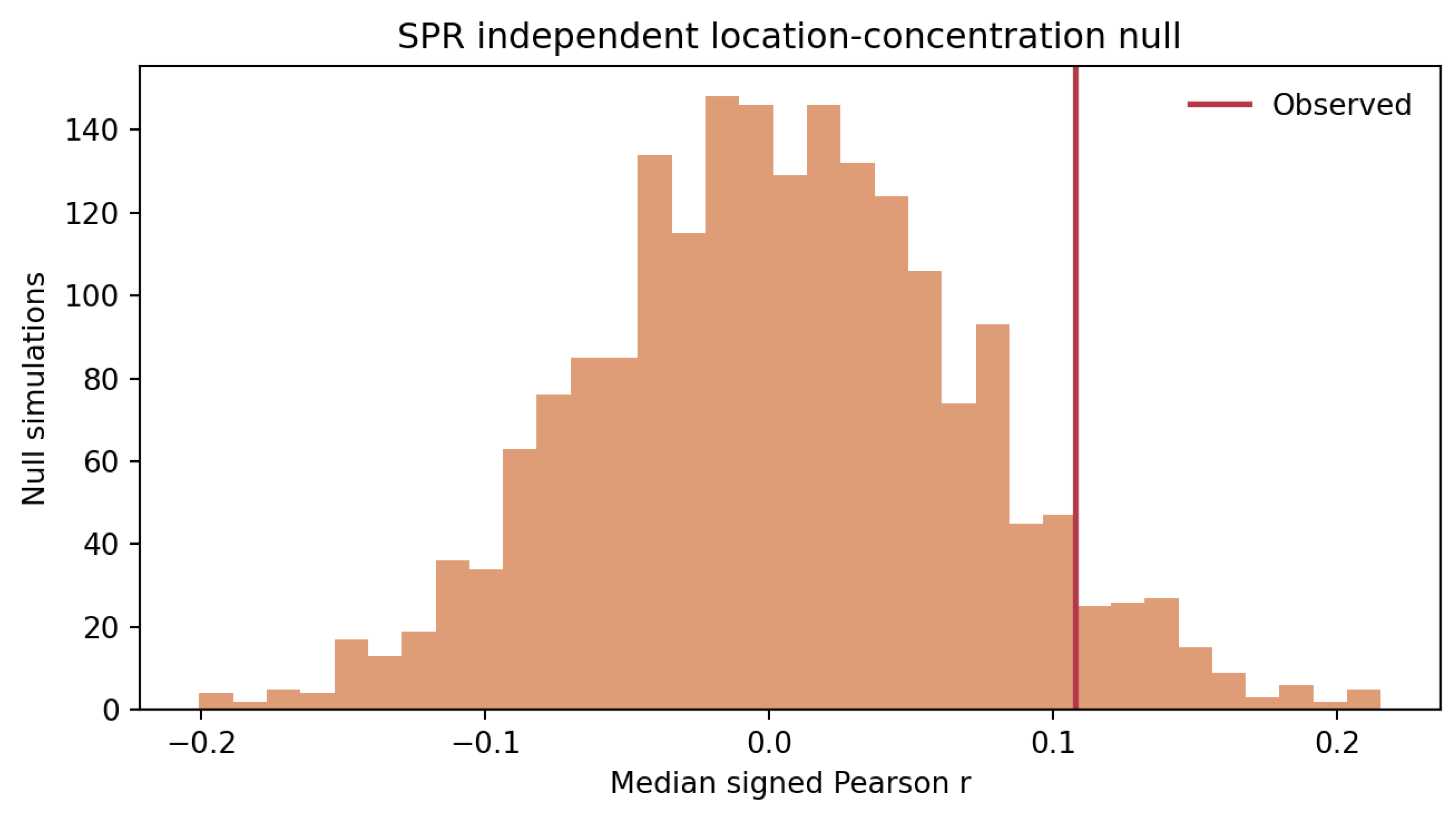
Table A58. Same-profile geometry diagnostics.

Surface	Observed statistic	Null summary	Probability	Conditioning	Role
ERP residual geometry	Median signed $r=.760004$	Median .661338; 95% interval [.598854, .729498]	.004498	Residual derangements, rejection, clipping, admissibility	Supporting excess over declared synthesis
SPR direction–concentration geometry	Median signed $r\approx .103$	Median .0029; 95% interval [-.1268, .1400]	.0610	Simplex construction and radius capping	Upper-tail, nondecisive diagnostic

Table A58. Same-profile geometry diagnostics.

Surface	Observed statistic	Null summary	Probability	Conditioning	Role
ERP residual geometry	Median signed $r=.760004$	Median .661338; 95% interval [.598854, .729498]	.004498	Residual derangements, rejection, clipping, admissibility	Supporting excess over declared synthesis
SPR direction–concentration geometry	Median signed $r\approx .103$	Median .0029; 95% interval [-.1268, .1400]	.0610	Simplex construction and radius capping	Upper-tail, nondecisive diagnostic

Appendix G.9. Combined Interpretation

The auxiliary diagnostics do not form a second claims ladder. They explain the transformation pattern supporting the primary results.

Pooling shows that a detailed population surface can survive after the observer relation has become undefined.

Observer reassignment shows that correct identity correspondence matters beyond the observed marginal values.

Desynchronization and gradient erasure show that temporal alignment and early-to-late organization support auxiliary same-profile operator recovery on the tested ERP surface.

The speed and total-cost controls identify serious behavioral reductions, while the absence of observer-separated coefficients keeps those reductions outside the final claim.

Same-profile geometry establishes that strong relations exist within the measured surfaces and, under specified models, can exceed constrained synthetic alternatives. It also explains why same-profile evidence alone is insufficient.

Together, the diagnostics support one bounded conclusion: observer identity and temporal organization carry information that population averaging, random correspondence, and targeted temporal destruction do not preserve.

Appendix H.1. Status of the Predictions

A prospective prediction enters this appendix only when it specifies:

1.

the scientific object to be recovered;

2.

the transformation or surface being compared;

3.

the coordinates held constant;

4.

the coordinate deliberately changed;

5.

the predicted ordering of the results;

6.

the result that would count against the prediction.

These are open experimental claims. Their presence here does not convert the current transformation pattern into prospective confirmation.

Appendix H.2. Matched Transformation Tests

The first comparison class holds information loss approximately constant while changing the structure preserved by the operator.

Appendix H.2.1. Order-Preserving Versus Order-Destroying Compression

The present three-bin operator preserves early, middle, and late order. A decisive comparison requires another three-category operator that retains the same cardinality and comparable marginal occupancy while destroying temporal order.

Let $Q_{\mathrm{ord}}$ denote an order-preserving compression and $Q_{\mathrm{scr}}$ an order-destroying compression. Both should return the same number of timing categories.

The prospective prediction is:

$$R\left(Q_{\mathrm{ord}}\left({\mathcal{S}}_i\right)\right)>R\left(Q_{\mathrm{scr}}\left({\mathcal{S}}_i\right)\right).$$

The result would support broad temporal order as part of the recoverable structure if observer-paired covariance survives ordered compression and declines under matched order destruction.

The prediction would fail if the two transformations produce comparable recovery, or if order destruction preserves more recovery than the ordered operator.

Appendix H.2.2. Sign-Preserving Versus Magnitude-Only Transformation

Signed temporal allocation and clipped concentration should be compared under the same observations, exposure requirements, lag positions, and reader strata.

Let $Q_{\pm }$ preserve positive and negative lag structure, and let $Q_{+}$ retain only nonnegative magnitude.

The prospective prediction is:

$$R\left(Q_{\pm }\left({\mathcal{S}}_i\right)\right)>R\left(Q_{+}\left({\mathcal{S}}_i\right)\right)$$

for operator pairs constructed to represent comparable temporal contrasts.

The prediction would support signed allocation as a stronger carrier if direction-preserving operators recover more observer-paired organization after reliability and exposure are matched.

It would fail if the magnitude-only family performs as well as or better than the signed family under those controls.

Appendix H.2.3. Identity-Preserving Versus Identity-Removing Compression

A further experiment should match temporal smoothing or dimensional reduction while changing whether observer identity remains available.

One transformation should compress each observer separately. The other should apply an equivalent reduction only after observers have been pooled.

The prediction is that the identity-preserving transformation will retain the observer relation, while the pooled transformation will retain only the population surface.

This experiment would test whether the pooling result generalizes beyond one averaging operation. It would fail if a population-level representation allows the same observer relation to be reconstructed without retaining observer-indexed quantities.

Appendix H.3. Same-Observer Cross-Surface Tests

The present ERP and self-paced reading results recur across measurement surfaces, but they do not recur within the same people. A same-observer study is required before neural and behavioral organization can be related directly.

Participants should complete:

• a semantic ERP task with sufficient trials for disjoint estimation;
• a dense behavioral task, preferably eye tracking, maze, or repeated self-paced reading;
• matched or closely related linguistic materials;
• at least two sessions when cross-session stability is part of the claim.

Neural timing and localization should be estimated from separate trial subsets. Behavioral timing and allocation should be estimated from separate items, stories, or sessions. Cross-modal prediction should then be evaluated on held-out observations.

Appendix H.3.1. Broad Neural Localization Versus Behavioral Allocation

The primary prediction is that neural early–late localization will predict signed behavioral allocation more strongly than native peak latency alone.

Formally, let $L_i^{\mathrm{ERP}}$ denote neural localization, $T_i^{\mathrm{ERP}}$ native neural timing, and $A_i^{\mathrm{beh}}$ signed behavioral allocation. The prediction is:

$$Rel\left(L_i^{\mathrm{ERP}},A_i^{\mathrm{beh}}\right)>Rel\left(T_i^{\mathrm{ERP}},A_i^{\mathrm{beh}}\right).$$

The comparison should use paired resampling because both coefficients involve the same observers.

The prediction would fail if native timing predicts behavioral allocation equally well or better, or if neither neural measure predicts behavior beyond reliability-matched nulls.

Appendix H.3.2. Within-Surface Recurrence Before Cross-Surface Prediction

Cross-modal prediction should be attempted only after each surface demonstrates observer-paired recurrence within the same sample.

The prospective sequence is:

1.

recover neural timing–localization covariance;

2.

recover behavioral timing–allocation covariance;

3.

test cross-modal correspondence;

4.

test prediction on held-out observers or sessions.

Failure at the first or second stage should not be repaired by searching for a cross-modal relation among unstable component estimates.

Appendix H.3.3. Cross-Session and Cross-Modal Structure

A stronger prediction is that observers with more stable within-surface organization across sessions will also show stronger neural-to-behavioral correspondence.

This would distinguish recurring observer organization from a relation driven primarily by one session’s noise, morphology, or task-specific strategy.

The prediction would fail if cross-session recurrence and cross-modal correspondence are unrelated.

Appendix H.4. Exposure-Balanced Behavioral Studies

Natural Stories provides broad naturalistic coverage but uneven reader exposure. An independent study should balance exposure before concentration and allocation are compared.

Each reader should contribute the same number of observations to:

• every temporal position;
• every condition;
• every partition side;
• each concentration and allocation operator;
• raw and transformed reading-time analyses, when both are retained.

Items should be assigned so that timing and localization can be estimated from disjoint but reliability-matched subsets.

Appendix H.4.1. Precision Under Balanced Exposure

The first prediction is that balanced exposure will narrow the reader-bootstrap interval for the behavioral family.

The relevant comparison is not the number of partition rows. It is the uncertainty of the family statistic under the same reader count, operator definitions, and resampling procedure.

The prediction would fail if balanced exposure produces no improvement in reader-sampling precision.

Appendix H.4.2. Allocation Versus Concentration

The second prediction is that signed allocation will retain stronger observer-paired recovery than nonnegative concentration when both are constructed from matched observations.

The study should prevent one family from receiving:

• more items;
• more reliable lags;
• more complete readers;
• more favorable exclusions;
• a larger operator grid.

A stronger signed result under those conditions would support a real distinction between temporal allocation and concentration.

The prediction would fail if the difference disappears after exposure and reliability are balanced.

Appendix H.4.3. Current-Word and Spillover Manipulation

A controlled behavioral experiment should manipulate where processing demand is expected to appear while holding total difficulty as stable as possible.

One condition should encourage immediate resolution. Another should delay resolution into spillover without increasing total processing cost by the same amount.

The prediction is that the manipulation will alter signed allocation more clearly than concentration. Observers should retain stable relative placement across disjoint item sets even when total cost is similar.

The prediction would fail if the manipulation changes only gross cost or if observer ordering does not recur across item sets.

Appendix H.5. Prospective Prediction Registry

Table A59. Open predictions generated by the present results.

ID	Experimental comparison	Prospective prediction	Result that would count against it	Status
H1	Order-preserving versus order-destroying compression at matched cardinality	Ordered compression retains greater observer recovery	Comparable or stronger recovery after order destruction	Open
H2	Sign-preserving versus magnitude-only behavioral operators	Signed allocation retains stronger reader-paired organization	Difference disappears or reverses under matched data	Open
H3	Identity-preserving versus pooled reduction	Within-observer reduction retains the relation; pooling does not	Observer relation recovered without an observer-indexed surface	Open
H4	Neural localization versus native latency as predictors of behavioral allocation	Broad neural localization predicts behavioral allocation more strongly	Native latency performs equally well or better	Open
H5	Cross-session stability and cross-modal prediction	Stable within-surface observers show stronger cross-modal correspondence	Cross-session and cross-modal organization are unrelated	Open
H6	Balanced versus uneven behavioral exposure	Balanced exposure narrows uncertainty and clarifies allocation–concentration differences	Precision and operator contrast do not improve	Open
H7	Immediate versus spillover-biased processing under matched total cost	Manipulation changes signed allocation more clearly than concentration	Only total cost changes, or observer ordering does not recur	Open

Table A59. Open predictions generated by the present results.

ID	Experimental comparison	Prospective prediction	Result that would count against it	Status
H1	Order-preserving versus order-destroying compression at matched cardinality	Ordered compression retains greater observer recovery	Comparable or stronger recovery after order destruction	Open
H2	Sign-preserving versus magnitude-only behavioral operators	Signed allocation retains stronger reader-paired organization	Difference disappears or reverses under matched data	Open
H3	Identity-preserving versus pooled reduction	Within-observer reduction retains the relation; pooling does not	Observer relation recovered without an observer-indexed surface	Open
H4	Neural localization versus native latency as predictors of behavioral allocation	Broad neural localization predicts behavioral allocation more strongly	Native latency performs equally well or better	Open
H5	Cross-session stability and cross-modal prediction	Stable within-surface observers show stronger cross-modal correspondence	Cross-session and cross-modal organization are unrelated	Open
H6	Balanced versus uneven behavioral exposure	Balanced exposure narrows uncertainty and clarifies allocation–concentration differences	Precision and operator contrast do not improve	Open
H7	Immediate versus spillover-biased processing under matched total cost	Manipulation changes signed allocation more clearly than concentration	Only total cost changes, or observer ordering does not recur	Open

Appendix H.6. Prospective Status Boundary

The present paper establishes that observer-paired ERP recovery survives one order-preserving compression and that signed behavioral allocation reveals strong reader organization under one naturalistic corpus.

It does not establish:

• that temporal order is the unique carrier;
• that signed allocation will dominate concentration in a balanced experiment;
• that neural and behavioral organization correspond within the same observer;
• that the relations are stable across sessions;
• that exposure balancing will necessarily strengthen the behavioral result.

Those are the next adjudications. They remain prospective until tested on independent data under declared operators.

Appendix I.1. Repository and Archive Navigation

The GitHub repository supports browsing and ongoing access. The Zenodo record is the permanent citation for the canonical release.

Table A60. Canonical release and archive records.

Record	Identifier or location
Repository	https://github.com/evlocoo/ODER-linguistics-empirical
GitHub release	https://github.com/evlocoo/ODER-linguistics-empirical/releases/tag/v1.0.0
Permanent archive	https://doi.org/10.5281/zenodo.22348751
Version	v1.0.0
Release date	September 5, 2026
Commit	34d0b9fc7f51126e1bf92ed901fe55defb019234
License	MIT

Table A60. Canonical release and archive records.

Record	Identifier or location
Repository	https://github.com/evlocoo/ODER-linguistics-empirical
GitHub release	https://github.com/evlocoo/ODER-linguistics-empirical/releases/tag/v1.0.0
Permanent archive	https://doi.org/10.5281/zenodo.22348751
Version	v1.0.0
Release date	September 5, 2026
Commit	34d0b9fc7f51126e1bf92ed901fe55defb019234
License	MIT

Appendix I.2. Status Definitions

Scientific status describes the role of the analysis:

• Primary locked: carries a central empirical claim.
• Supporting: tests stability or a declared reduction without replacing the primary analysis.
• Frozen prospective: contrast and interpretation fixed before outcome inspection.
• Prospectively specified secondary: added under a written protocol to test a distinct sensitivity.
• Deterministic diagnostic: alters one coordinate without adding a resampling claim.
• Selected-profile diagnostic: restricted by observed profile properties.
• Post-diagnostic: performed after an implementation feature was identified.
• Provenance: establishes input or construction identity rather than an effect.

Verification result records whether the artifact reproduces the expected manuscript value:

• Matched: output equals the expected value within the declared reporting precision.
• Structural: the result concerns definability or preserved structure rather than one scalar estimate.

Integrity status records artifact condition:

• PASS: required notebook, output, and verification record are present and internally consistent.
• MISSING: a required artifact is absent.

Appendix I.3. ERP Primary and Destructive-Control Claims

Appendix I.3.1. I-E1. ERP Provenance and Locked Split

Field	Manifest record
Manuscript location	Sections 4.2–4.5; Appendix B.1–B.4
Scientific status	Provenance
Notebook	notebooks/source/00AERPSurfaceandOperatorVerification.ipynb; notebooks/source/01ERPObserverSeparatedRecovery.ipynb
Notebook section	Source verification; trial eligibility; locked condition-stratified split
Output file	outputs/erp/surface/erpsurfaceinputaudit.csv; outputs/erp/erpcrossfitsplitregistry.csv; outputs/erp/erpprimarylockedtrialindices.csv
Figure or table	Appendix B, Tables B1–B4
Expected value	40 participants; 60 expected and 60 unexpected trials per participant; 30 trials per condition in each half; 4,800 assignment rows; 80 of 80 participant-condition half hashes reproduced
Verification result	Matched
Integrity status	PASS

Appendix I.3.2. I-E2. Locked Bidirectional ERP Recovery

Field	Manifest record
Manuscript location	Sections 5.1 and 5.6; Appendix B.5–B.8; Appendix F.1
Scientific status	Primary locked
Notebook	notebooks/source/01ERPObserverSeparatedRecovery.ipynb
Notebook section	Primary rectified construction; bidirectional cross-fit; shared observer inference
Output file	outputs/erp/erpcrossfitresults.csv; outputs/erp/erpcrossfitsummary.csv; outputs/erp/erpcrossfitbootstrap.csv; outputs/erp/erpcrossfitpermutationnull.csv
Figure or table	Primary ERP reconstruction figure; Table 3; Appendix B, Table B5
Expected value	$A\to B=.442$; $B\to A=.343$; symmetric Pearson $r=.393$; 95% interval $[.207,.554]$; shared-pairing $p=.0004$; symmetric Spearman $\rho =.413$
Verification result	Matched
Integrity status	PASS

Appendix I.3.3. I-E3. Repeated-Split Stability and Amplitude Reduction

Field	Manifest record
Manuscript location	Sections 5.5–5.6; Appendix B.9–B.10
Scientific status	Supporting
Notebook	notebooks/source/01ERPObserverSeparatedRecovery.ipynb
Notebook section	Repeated condition-stratified splits; amplitude-controlled reduction
Output file	outputs/erp/erpcrossfitrepeatedsplits.csv; outputs/erp/erpcrossfitsummary.csv
Figure or table	Repeated-split recurrence figure; Table 3; Appendix B, Table B5
Expected value	Amplitude-controlled symmetric $r=.431$; repeated-split median $r=.305$; quartiles $[.256,.361]$; all 200 estimates positive
Verification result	Matched
Integrity status	PASS

Appendix I.3.4. I-E4. Pooling Removes the Observer Estimand

Field	Manifest record
Manuscript location	Sections 1.2, 5.2, and 8.2; Appendices G.1–G.2
Scientific status	Deterministic diagnostic
Notebook	supportingsameprofile/notebooks/source/ODERERPN400verificationcorrectedv2.ipynb
Notebook section	Pooling diagnostic
Output file	supportingsameprofile/outputs/erp/erpsubjectmetrics.csv; supportingsameprofile/outputs/erp/figures/08pooling.png
Figure or table	ERP pooling figure; Appendix G, Tables G1–G2
Expected value	Canonical group semantic-negativity surface preserved; participant-indexed timing–localization relation undefined after pooling
Verification result	Structural
Integrity status	PASS

Appendix I.3.5. I-E5. Desynchronization Collapses Same-Profile Operator Recovery

Field	Manifest record
Manuscript location	Sections 5.3 and 8.1; Appendix G.4
Scientific status	Deterministic destructive diagnostic
Notebook	supportingsameprofile/notebooks/source/ODERERPN400verificationcorrectedv2.ipynb
Notebook section	Operator desynchronization sweep
Output file	supportingsameprofile/outputs/erp/erpdesyncsweep.csv; supportingsameprofile/outputs/erp/erpdesyncperspec.csv
Figure or table	Figure 3; Appendix G.4
Expected value	Aligned formula-distinct family median approximately $r=.620$; $\pm 250$-ms desynchronized median approximately $r=.005$; predicted-direction preservation approximately 31.9%
Verification result	Matched
Integrity status	PASS

Appendix I.3.6. I-E6. Temporal-Gradient Erasure Collapses Same-Profile Operator Recovery

Field	Manifest record
Manuscript location	Sections 5.3 and 8.1; Appendix G.5
Scientific status	Deterministic destructive diagnostic
Notebook	supportingsameprofile/notebooks/source/ODERERPN400verificationcorrectedv2.ipynb
Notebook section	Verification of frozen original-run strict-window detrend control
Output file	supportingsameprofile/outputs/erp/erpwindowsensitivity.csv
Figure or table	Appendix G.5
Expected value	Strict-window median approximately $r=.638$ before detrending and $r=.010$ after gradient erasure
Verification result	Frozen original-run artifact matched
Integrity status	PASS

Appendix I.4. Frozen Temporal-Compression Claims

Appendix I.4.1. I-P1. Frozen Native-Versus-Three-Bin Contrast

Field	Manifest record
Manuscript location	Sections 7.1–7.2; Appendix D.1–D.9
Scientific status	Frozen prospective
Notebook	notebooks/source/04ERPTemporalCompression.ipynb
Notebook section	Frozen focal contrast; shared bootstrap and permutation
Output file	outputs/phase3/erpphase3frozencontrastsummary.csv; outputs/phase3/erpphase3contrastbootstrap.csv; outputs/phase3/erpphase3contrastpermutations.csv
Figure or table	Focal compression figure; Table 6; Appendix D, Tables D5 and D8
Expected value	Native $r=.393$; three-bin $r=.396$; native-minus-three-bin $\Delta z=-.0035$; 95% interval $[-.155,.172]$; one-sided $p=.510$
Verification result	Matched; frozen prediction not supported
Integrity status	PASS

Appendix I.4.2. I-P2. Full Compression Ladder and Identifiability

Field	Manifest record
Manuscript location	Sections 7.3–7.5; Appendix D.4–D.13
Scientific status	Frozen extension and supporting diagnostic
Notebook	notebooks/source/04ERPTemporalCompression.ipynb
Notebook section	Full resolution ladder; metric identifiability; repeated splits
Output file	outputs/phase3/erpphase3resolutionsummary.csv; outputs/phase3/erpphase3metricidentifiability.csv; outputs/phase3/erpphase3repeatedsplitresults.csv
Figure or table	Compression-coordinate figure; full-ladder figure; Appendix D, Tables D5–D9
Expected value	Ladder $r=.393,.374,.365,.396,.396,.395$; finite slope (-.0105), interval $[-.0520,.0394]$, $p=.643$; cardinality $34.5\to 3$; repeated-split native median .305 and three-bin median .343
Verification result	Matched
Integrity status	PASS

Appendix I.4.3. I-P3. Flat-Profile Tie Sensitivity

Field	Manifest record
Manuscript location	Section 7.6; Appendix D.15
Scientific status	Post-diagnostic
Computation	tools/phase3tiesensitivity.py
Computation section	Flat-profile exclusion and native-tie harmonization sensitivities
Output file	outputs/phase3/erpphase3tiesensitivity.csv
Figure or table	Appendix D, Table D10
Expected value	Excluding sub-040: $\Delta z=.0098$, interval $[-.1457,.1881]$, $p=.448$; mean tied native location: $\Delta z=.0096$, interval $[-.1396,.1828]$, $p=.446$
Verification result	Matched; no change to frozen conclusion
Integrity status	PASS

Appendix I.5. Unrectified ERP Sensitivity

Appendix I.5.1. I-U1. ERP Recovery Without Zero Rectification

Field	Manifest record
Manuscript location	Sections 5.4 and 7.4; Appendices B.11–B.14 and D.11–D.12
Scientific status	Prospectively specified secondary
Notebook	secondarysensitivities/notebooks/source/01UnrectifiedERPSensitivity.ipynb
Notebook section	Unrectified recovery and compression
Output file	secondarysensitivities/outputs/erp/erpunrectifiedcanonicaldirectionalresults.csv; secondarysensitivities/outputs/erp/erpunrectifiedresolutionsummary.csv; secondarysensitivities/outputs/erp/erpunrectifiedfrozencontrastsummary.csv; secondarysensitivities/outputs/erp/erpunrectifiedsharedobserverbootstrap.csv; secondarysensitivities/outputs/erp/erpunrectifiedsharedsubjectpermutations.csv
Figure or table	Unrectified ERP figure; Appendix B, Table B6; Appendix D, Tables D7–D8
Expected value	Native $r=.330$, interval $[.060,.561]$, $p=.0026$; three-bin $r=.333$, interval $[.058,.566]$, $p=.0024$; native-minus-three-bin $\Delta z=-.0037$, interval $[-.207,.196]$, $p=.511$
Verification result	Matched
Integrity status	PASS

Appendix I.5.2. I-U2. Rectified-Minus-Unrectified Comparison

Field	Manifest record
Manuscript location	Sections 5.4 and 7.4; Appendix B.14
Scientific status	Prospectively specified secondary
Notebook	secondarysensitivities/notebooks/source/01UnrectifiedERPSensitivity.ipynb
Notebook section	Unrectified recovery and compression; paired surface comparison
Output file	secondarysensitivities/outputs/erp/erprectifiedvsunrectifiedcomparison.csv; secondarysensitivities/outputs/erp/erprectifiedminusunrectifiedpairedbootstrap.csv
Figure or table	Rectification comparison figure; Appendix B, Table B7
Expected value	Native rectified-minus-unrectified $\Delta z=.073$, interval $[-.081,.250]$; focal compression-contrast difference approximately .00016
Verification result	Matched; removal of rectification preserves recovery, equivalence not established
Integrity status	PASS

Appendix I.6. Natural Stories Provenance and Behavioral Claims

Appendix I.6.1. I-S1. Corpus, Surprisal, Alignment, and Exposure

Field	Manifest record
Manuscript location	Sections 4.7–4.8 and 6.1; Appendix C.1–C.6
Scientific status	Provenance and primary boundary
Notebook	notebooks/source/00BSPRSurfaceandOperatorVerification.ipynb; notebooks/source/02SPRObserverSeparatedRecovery.ipynb
Notebook section	Corpus ingestion; surprisal alignment; reader exposure; partition registry
Output file	outputs/spr/surface/sprsurfaceinputaudit.csv; outputs/spr/sprcrossfitobserverstrata.csv; outputs/spr/sprcrossfitreaderstorytokencoverage.csv; source-dataset surprisal artifact probs/allstoriesgpt3.csv (not redistributed)
Figure or table	Appendix C, Tables C1–C5
Expected value	10 stories; 10,256 displayed words; 10,255 exact alignments; 1 approximate alignment; 0 failures; 180 readers; 848,875 aligned rows; 125 locked scored partitions; 96-reader common stratum; complete exposure 7.25% on side A and 7.36% on side B
Verification result	Matched
Integrity status	PASS

Appendix I.6.2. I-S2. Locked Clipped Concentration Family

Field	Manifest record
Manuscript location	Sections 6.1 and 6.5; Appendix C.8 and Appendix F.4
Scientific status	Primary locked behavioral family
Notebook	notebooks/source/02SPRObserverSeparatedRecovery.ipynb
Notebook section	Complementary-story cross-fit; locked clipped family inference
Output file	outputs/spr/sprcrossfitfamilysummary.csv; outputs/spr/sprcrossfitdirectionalstatistics.csv; outputs/spr/sprcrossfitfamilybootstrap.csv; outputs/spr/sprcrossfitfamilypermutationnull.csv
Figure or table	Clipped-family figure; behavioral surface comparison table; Appendix C, Table C6
Expected value	96 readers; 125 partitions; 10 specifications; 1,250 dependent estimates; family median $r=.103$; interval $[-.026,.297]$; pairing $p=.0162$; predicted-direction preservation 88.88%
Verification result	Matched
Integrity status	PASS

Appendix I.6.3. I-S3. Clipping Eligibility Audit

Field	Manifest record
Manuscript location	Section 6.2; Appendix C.9
Scientific status	Deterministic diagnostic
Notebook	secondarysensitivities/notebooks/source/02SPRClippingandSignedSlopeSensitivity.ipynb
Notebook section	Raw slopes, clipping audit, and signed-safe recovery
Output file	secondarysensitivities/outputs/spr/sprclippingprofilestatus.csv; secondarysensitivities/outputs/spr/sprclippingprofilecountdistribution.csv; secondarysensitivities/outputs/spr/sprclippingprofilesummary.csv
Figure or table	Appendix C, Table C7
Expected value	Eligible denominator 48,218; 41,280 profiles with zero clipped positions; 6,200 with one; 738 with two; 0 with three
Verification result	Matched
Integrity status	PASS

Appendix I.6.4. I-S4. Signed-Safe Temporal-Allocation Family

Field	Manifest record
Manuscript location	Sections 6.3 and 8.3; Appendix C.10–C.12; Appendix F.5
Scientific status	Prospectively specified secondary
Notebook	secondarysensitivities/notebooks/source/02SPRClippingandSignedSlopeSensitivity.ipynb
Notebook section	Raw slopes, clipping audit, and signed-safe recovery
Output file	secondarysensitivities/outputs/spr/sprsignedsafecrossfitresults.csv; secondarysensitivities/outputs/spr/sprsignedsafereaderstrata.csv; secondarysensitivities/outputs/spr/sprsignedsafesharedbootstrap.csv; secondarysensitivities/outputs/spr/sprsignedsafesharedpermutation.csv; secondarysensitivities/outputs/spr/sprsecondarysensitivitysummary.csv
Figure or table	Signed-family figure; Appendix C, Tables C8–C10; Appendix F, Table F5
Expected value	96 readers; 125 partitions; 6 specifications; 750 dependent estimates; all specification medians positive, range .415–.709; family median $r=.491$; interval $[.407,.577]$; pairing $p=.0002$; 100% direction preservation
Verification result	Matched
Integrity status	PASS

Appendix I.6.5. I-S5. Clipping-Inactive Selected-Profile Family

Field	Manifest record
Manuscript location	Section 6.4; Appendix C.13; Appendix F.6
Scientific status	Selected-profile diagnostic
Notebook	secondarysensitivities/notebooks/source/02SPRClippingandSignedSlopeSensitivity.ipynb
Notebook section	Raw slopes, clipping audit, and signed-safe recovery
Output file	secondarysensitivities/outputs/spr/sprnoclippingsubsetcrossfitresults.csv; secondarysensitivities/outputs/spr/sprnoclippingsubsetreaderstrata.csv; secondarysensitivities/outputs/spr/sprnoclippingsubsetsharedbootstrap.csv; secondarysensitivities/outputs/spr/sprnoclippingsubsetsharedpermutation.csv
Figure or table	Figure 5B; Appendix C, Tables C11–C12; Appendix F, Table F6
Expected value	Two strata of 33 and 31 readers; 125 scored partitions; 10 specifications; family median $r=.206$; interval $[.044,.363]$; pairing $p=.0002$; 94.24% direction preservation
Verification result	Matched
Integrity status	PASS

Appendix I.7. Manifest Summary

Table A77. Major claim status.

ID	Claim	Scientific status	Verification	Integrity
I-E1	ERP source and fixed split	Provenance	Matched	PASS
I-E2	Locked bidirectional ERP recovery	Primary locked	Matched	PASS
I-E3	Repeated splits and amplitude reduction	Supporting	Matched	PASS
I-E4	Pooling removes observer estimand	Deterministic diagnostic	Structural	PASS
I-E5	Desynchronization collapses same-profile operator recovery	Destructive diagnostic	Matched	PASS
I-E6	Gradient erasure collapses same-profile operator recovery	Destructive diagnostic	Frozen original-run artifact matched	PASS
I-P1	Native-versus-three-bin contrast	Frozen prospective	Matched, prediction failed	PASS
I-P2	Full ladder and identifiability	Frozen extension	Matched	PASS
I-P3	Flat-profile tie sensitivity	Post-diagnostic	Matched	PASS
I-U1	Unrectified ERP recovery	Secondary	Matched	PASS
I-U2	Rectification comparison	Secondary	Matched	PASS
I-S1	Corpus, alignment, and exposure	Provenance and boundary	Matched	PASS
I-S2	Locked clipped family	Primary locked behavioral	Matched	PASS
I-S3	Clipping eligibility audit	Deterministic diagnostic	Matched	PASS
I-S4	Signed-safe family	Secondary	Matched	PASS
I-S5	Clipping-inactive family	Selected diagnostic	Matched	PASS

Table A77. Major claim status.

ID	Claim	Scientific status	Verification	Integrity
I-E1	ERP source and fixed split	Provenance	Matched	PASS
I-E2	Locked bidirectional ERP recovery	Primary locked	Matched	PASS
I-E3	Repeated splits and amplitude reduction	Supporting	Matched	PASS
I-E4	Pooling removes observer estimand	Deterministic diagnostic	Structural	PASS
I-E5	Desynchronization collapses same-profile operator recovery	Destructive diagnostic	Matched	PASS
I-E6	Gradient erasure collapses same-profile operator recovery	Destructive diagnostic	Frozen original-run artifact matched	PASS
I-P1	Native-versus-three-bin contrast	Frozen prospective	Matched, prediction failed	PASS
I-P2	Full ladder and identifiability	Frozen extension	Matched	PASS
I-P3	Flat-profile tie sensitivity	Post-diagnostic	Matched	PASS
I-U1	Unrectified ERP recovery	Secondary	Matched	PASS
I-U2	Rectification comparison	Secondary	Matched	PASS
I-S1	Corpus, alignment, and exposure	Provenance and boundary	Matched	PASS
I-S2	Locked clipped family	Primary locked behavioral	Matched	PASS
I-S3	Clipping eligibility audit	Deterministic diagnostic	Matched	PASS
I-S4	Signed-safe family	Secondary	Matched	PASS
I-S5	Clipping-inactive family	Selected diagnostic	Matched	PASS

Appendix I.8. Machine-Readable Manifest

The release records the operational dependency and integrity fields in:

manifests/claimtoartifactmanifest.csv

The paper-facing labels map to machine-readable claim IDs as follows: I-E1 to ERP-PROV1; I-E2 to ERP-CF1; I-E3 to ERP-RS1 and ERP-AMP1; I-E4 to ERP-POOL1; I-E5 to ERP-DESYNC1; I-E6 to ERP-GRAD1; I-P1 to P3-CON1; I-P2 to P3-LAD1; I-P3 to P3-TIE1; I-U1 to SEC-ERP-UNRECT1; I-U2 to SEC-ERP-RECT1; I-S1 to SPR-COV1; I-S2 to SPR-FAM1; I-S3 to SEC-SPR-CLIP1; I-S4 to SEC-SPR-SIGNED1; and I-S5 to SEC-SPR-NOCLIP1.

The CSV contains one row per machine-readable claim and the following fields:

• claim_id;
• manuscript_location;
• source_notebook;
• notebook_stage;
• output_file;
• exact_output_columns_or_rows;
• scientific_status;
• protocol_config_identifier;
• figure_generation_source;
• integrity_status.

When one claim depends on more than one output, the file field uses a pipe-delimited list. The release verifier checks every listed notebook and output path, required schema, and declared numerical result.

The manifest is complete only when every manuscript-grade numerical claim can be traced from prose to a released notebook and from that notebook to a machine-readable output.

References

- Beatty, J. Task-evoked pupillary responses, processing load, and the structure of processing resources. Psychol. Bull. 1982, 91(2), 276–292. [Google Scholar] [CrossRef]
- Clayson, P. E.; Miller, G. A. Psychometric considerations in the measurement of event-related brain potentials: Guidelines for measurement and reporting. Int. J. Psychophysiol. 2017, 111, 57–67. [Google Scholar] [CrossRef] [PubMed]
- Cooper, E., III. Observer-dependent entropy retrieval in linguistic comprehension: A bounded-access theory of semantic timing, reanalysis, and collapse; Preprint, 2026. [Google Scholar] [CrossRef]
- Cooper, E. Relational observability of semantic timing: What pooling erases and temporal compression preserves (Version 1.0.0) [Software]. Zenodo 2026. [Google Scholar] [CrossRef]
- Di Liberto, G. M.; O’Sullivan, J. A.; Lalor, E. C. Low-frequency cortical entrainment to speech reflects phoneme-level processing. Curr. Biol. 2015, 25(19), 2457–2465. [Google Scholar] [CrossRef] [PubMed]
- Fisher, A. J.; Medaglia, J. D.; Jeronimus, B. F. Lack of group-to-individual generalizability is a threat to human subjects research. Proc. Natl. Acad. Sci. 2018, 115(27), E6106–E6115. [Google Scholar] [CrossRef] [PubMed]
- Futrell, R.; Gibson, E.; Tily, H. J.; Blank, I. A.; Vishnevetsky, A.; Piantadosi, S. T.; Fedorenko, E. The Natural Stories corpus. In Proceedings of the Eleventh International Conference on Language Resources and Evaluation (LREC 2018); European Language Resources Association, 2018; Available online: https://aclanthology.org/L18-1012/.
- Futrell, R.; Gibson, E.; Tily, H. J.; Blank, I. A.; Vishnevetsky, A.; Piantadosi, S. T.; Fedorenko, E. The Natural Stories corpus: A reading-time corpus of English texts containing rare syntactic constructions. Lang. Resour. Eval. 2021, 55, 63–77. [Google Scholar] [CrossRef] [PubMed]
- Hale, J. A probabilistic Earley parser as a psycholinguistic model. In Proceedings of the Second Meeting of the North American Chapter of the Association for Computational Linguistics, 2001. [Google Scholar] [CrossRef]
- Hedge, C.; Powell, G.; Sumner, P. The reliability paradox: Why robust cognitive tasks do not produce reliable individual differences. Behav. Res. Methods 2018, 50, 1166–1186. [Google Scholar] [CrossRef] [PubMed]
- Kappenman, E. S.; Farrens, J. L.; Zhang, W.; Stewart, A. X.; Luck, S. J. ERP CORE [Data set and analysis resources]. In Open Science Framework; 2020. [Google Scholar] [CrossRef]
- Kappenman, E. S.; Farrens, J. L.; Zhang, W.; Stewart, A. X.; Luck, S. J. ERP CORE: An open resource for human event-related potential research. NeuroImage 2021, 225, 117465. [Google Scholar] [CrossRef] [PubMed]
- Kutas, M.; Hillyard, S. A. Reading senseless sentences: Brain potentials reflect semantic incongruity. Science 1980, 207(4427), 203–205. [Google Scholar] [CrossRef] [PubMed]
- Kutas, M.; Federmeier, K. D. Thirty years and counting: Finding meaning in the N400 component of the event-related brain potential. Annu. Rev. Psychol. 2011, 62, 621–647. [Google Scholar] [CrossRef] [PubMed]
- Levy, R. Expectation-based syntactic comprehension. Cognition 2008, 106(3), 1126–1177. [Google Scholar] [CrossRef] [PubMed]
- Luck, S. J. An introduction to the event-related potential technique, 2nd ed.; MIT Press, 2014; Available online: https://mitpress.mit.edu/9780262525855/an-introduction-to-the-event-related-potential-technique/.
- Molenaar, P. C. M. A manifesto on psychology as idiographic science: Bringing the person back into scientific psychology, this time forever. Meas. Interdiscip. Res. Perspect. 2004, 2(4), 201–218. [Google Scholar] [CrossRef] [PubMed]
- Rayner, K. Eye movements in reading and information processing: 20 years of research. Psychol. Bull. 1998, 124(3), 372–422. [Google Scholar] [CrossRef] [PubMed]
- Rouder, J. N.; Haaf, J. M. A psychometrics of individual differences in experimental tasks. Psychon. Bull. Rev. 2019, 26, 452–467. [Google Scholar] [CrossRef] [PubMed]
- Smith, N. J.; Levy, R. The effect of word predictability on reading time is logarithmic. Cognition 2013, 128(3), 302–319. [Google Scholar] [CrossRef] [PubMed]
- Winn, M. B.; Wendt, D.; Koelewijn, T.; Kuchinsky, S. E. Best practices and advice for using pupillometry to measure listening effort: An introduction for those who want to get started. Trends Hear. 2018, 22, 2331216518800869. [Google Scholar] [CrossRef] [PubMed]
Disclaimer/Publisher’s Note: The statements, opinions and data contained in all publications are solely those of the individual author(s) and contributor(s) and not of MDPI and/or the editor(s). MDPI and/or the editor(s) disclaim responsibility for any injury to people or property resulting from any ideas, methods, instructions or products referred to in the content. |
© 2026 by the author. Licensee MDPI, Basel, Switzerland. This article is an open access article distributed under the terms and conditions of the Creative Commons Attribution (CC BY) license.
Copyright: This open access article is published under a Creative Commons CC BY 4.0 license, which permit the free download, distribution, and reuse, provided that the author and preprint are cited in any reuse.