

Submitted:
12 September 2026
Posted:
15 September 2026
You are already at the latest version
Abstract
Classical theories typically model a complete record as a unary function of a physical state, treating observation conditions as external parameters. However, quantum mechanics exhibits a fundamental tension: the same independently certified physical input can yield different complete records when observation conditions vary, giving rise to the century-old measurement problem and the EPR paradox. In this work, we derive the necessary state architecture to resolve this without conflating the physical input with the conditions through which its record is formed. By applying behavioral equivalence and redundancy elimination within the category of sets, we prove that the formation-side difference cannot be mathematically removed. This forces the “observation state” to emerge as an irreducible, objective, state-bearing axis, establishing a strict physical–observation dual-axis (PODA) architecture. We emphasize that this dual-axis structure represents two non-interchangeable projection responsibilities, rather than orthogonal coordinates or dynamically decoupled systems. Under stated coherence and composition conditions, this dual-axis geometry naturally yields the complex field, binary projective geometry, and the Born trace pairing. Crucially, it further derives the Schrödinger equation as a covariant temporal composition, the CHSH inequality, and the attainable Tsirelson bound. In standard quantum mechanics, the complex field,theSchrödingerequation, and the Born rule are independent axioms. In our framework, they are unified as geometric corollaries of the PODA structure. Within this framework, the notorious quantum paradoxes are naturally dissolved: “wave-function collapse” is revealed as a conditional transition at the observation interface, and “decoherence” is understood as the objective geometric coupling between the physical and observation axes, rather than random environmental noise. Bell violation is thereby identified not as superluminal influence, but as the absence of a positive global answer section across incompatible observation states. Finally, the theory proposes a specific table-top experiment that predicts a sharp, parameter-free numerical constant: a geometric phase of (0.7π ≈ 2.1991) radians. This value directly distinguishes the dual-axis mechanism from standard quantum mechanics, which predicts exactly zero for the same configuration. Observing this constant would confirm the physical reality of the observation axis, whereas a null result falsifies the mechanism.
Keywords:
PODA Theory
; PODA Axiom
; physical–observation dual axis
; categorical foundations
; observation state
; behavior-minimal realization
; quotient
; pullback
; phase transport
; identifiability
; geometric phase
1. Introduction
Quantum mechanics is one of the most successful theories in physics, yet it forces us to confront a profound rupture between physical reality and the conditions of its observation. This rupture lies at the very heart of the quantum foundations. Bohr insisted that observation conditions cannot be detached from the atomic phenomenon [9]. Einstein, Podolsky, and Rosen responded by placing completeness and separability at the core of reality [10], while Schrödinger revealed through entanglement that a composite state cannot be unraveled into autonomous parts [11]. What began as a conceptual impasse soon hardened into mathematical bounds. Bell, CHSH, and Kochen–Specker established exact constraints on context-independent assignments [12,13,14], and Tsirelson fixed the ultimate quantum operator boundary [48]. Today, operational reconstructions and categorical quantum mechanics strive to recover the Hilbert formalism from informational principles [18,19,20,21,22,23,24]. Yet, every one of these approaches takes a family of well-defined objects for granted. The decisive mystery remains untouched: how does a physical fact actually come into being?
Classical theories typically attempt to answer this by presupposing a fixed observational law. When the measurement rule, reference condition, and processing configuration remain fixed throughout the domain under study, a record written as
is not an approximation; it is a complete law on that fixed observational slice. Its boundary, however, becomes visible when the conditions of record formation begin to vary. If an identity certified independently by an antecedent physical theory remains fixed while the complete record changes, this law is no longer constant along the corresponding fibers of the first projection. The pressing question is not whether another variable can be appended to the notation, but whether the formation-side difference can be eliminated without altering any primitive fact. At this stage, such a difference has no state semantics; its mathematical identity remains to be established.
One might naturally seek a resolution within established mathematical frameworks. However, information theory, statistical inference, and decision theory ordinarily begin with random variables, channels, or statistical experiments that are already formed [1,2,3,15]. Measurement theory studies faithful representations of empirical relations [16]; experimental design treats the experimental condition as a controllable object [4,5]; and the theories of state-dependent channels and statistical experiments examine how a supplied state changes a channel and how experiments may be compared [6,7,8,17]. Every one of these frameworks presupposes a well-defined family of objects. Consequently, they bypass the most fundamental question: When reference phase, detector configuration, or another condition of record formation changes the record, how do the primitive facts themselves separate a change in what is observed from a change in how its fact is formed? And how can duplicate labels be removed without relying on conditions that agree only accidentally at a single input?
To resolve this, we must step back to a more primitive level of representation. Rather than appending variables to an ill-suited framework, we derive the state architecture directly from the requirement that complete behavior must distinguish between a change in what is observed and a change in how its fact is formed. To achieve this with absolute mathematical rigor, we employ the framework of category theory. Here, category theory is not an end in itself, but the proof instrument: it allows us to rigorously test whether the formation-side difference can be eliminated without discarding any primitive fact. The result is a striking conclusion: the act of observation is intrinsically non-trivial. The condition of record formation cannot be reduced to a passive readout or a mere redundancy. It must emerge as an irreducible, state-bearing physical responsibility. We term this the “Physical–Observation Dual-Axis” (PODA) architecture. Crucially, this PODA structure represents two non-interchangeable projection responsibilities; it does not mean two orthogonal coordinates, statistical independence, or dynamically decoupled systems. Only by establishing this ontological foundation can the quantum formalism—the complex field, the Born rule, and the deterministic single-event dynamics—be derived as natural consequences, rather than assumed as axioms.
This recognition of observational non-triviality dissolves the century-old quantum paradoxes. What standard theory labels as “wave-function collapse” is revealed to be a conditional transition at the interface of the two axes, and “decoherence” becomes the objective geometric coupling between them. The mathematical architecture of this PODA framework, rigorously constructed in the category of sets, demonstrates that observation is not a subjective intervention, but an irreducible state-bearing axis of the fundamental law itself. In this paper, we focus on the quantum realization of this architecture. The consequences for relativistic frame geometry and internal gauge physics, while highly suggestive, lie beyond our present scope. In the following sections, we develop the exact mathematical foundations of this PODA structure and derive its observable predictions.

Table 1.
Constructive stages and their categorical expressions. Behavioral reduction establishes the formation-side state identity step by step.
Table 1.
Constructive stages and their categorical expressions. Behavioral reduction establishes the formation-side state identity step by step.
| Structural question | Categorical construction | Exact criterion |
|---|---|---|
| Can the formation-side role be deleted? | Factorization | Test whether the complete law descends through the corresponding projection |
| Which raw labels may be merged? | Kernel pairs and coequalizers | Remove only labels with identical complete behavior |
| How is a redundancy-free realization obtained? | Regular epimorphism–monomorphism factorization and terminal object | Obtain the complete behavior-minimal realization and its unique compatible isomorphism |
| How do the reduced roles appear jointly? | Product | Pair two typed coordinate maps without asserting independence |
| Which joint points and comparisons are admissible? | Pullback | Construct the feasible domain, fixed-state slices, and same-source domain |
| What does one surviving formation class select? | Exponential transpose | Identify it with one complete response map |
| Once state identity is established, can it be recovered from an output? | Monomorphisms and descent | Separate conditional, label-free, and joint identifiability |
2. Primitive Observational Facts and Observational Nontriviality
2.1. The Exact Unary Law on a Fixed Formation Slice
Let us return to the classical single-axis law y=h(x) introduced earlier. In a realistic experimental setting, the physical preparation label p corresponds to x, while the record-forming conditions (e.g., reference phase, detector configuration) correspond to the external parameters implicitly encoded in the map h.
Consider first the simplest case: the record-forming condition is held fixed at some specific value , while the preparation label p is varied. Within this slice, the classical single-axis law remains perfectly valid, yielding the unary record law:
Proposition 1
(Exactness of a fixed formation slice). On the experimental domain in which remains fixed, the unary law is a complete representation of the record. The same statement holds when the complete record is a probability distribution or a channel rather than a scalar value.
Proof.
By definition, assigns to every permitted p precisely the complete record obtained under the fixed condition . Changing the type of that record does not alter this pointwise identity. □
Thus a unary physical law is exact whenever the formation condition is fixed. The new structural question begins only when the domain itself contains more than one such condition and the corresponding slices cease to agree.
2.2. The Preserved First Role and the Unclassified Formation Role
Throughout this work, we distinguish between physical reality as the ontological substrate of the world and physical state as the specific carrier instance of that reality within a concrete experiment. Both are represented mathematically by elements of the set (or ), and their identity is what remains invariant under the behavioral reduction.
The fundamental asymmetry originates from the experiment itself. The first set, , represents the labels of physical reality; their identity remains fixed as the observation conditions vary. A second set, , lists these observation conditions. At this stage, is merely a typed collection of conditions; it is not yet declared as a state space, nor do its distinct labels necessarily imply physically distinct states. The relation of to an antecedent physical state space is deferred to the later compatibility theorem. No intermediate state carrier is needed to formulate this primitive comparison.
This separation is indispensable. Equality in signifies that the identity of physical reality is preserved while an observation condition is varied; equality in signifies that the same observation condition is compared across different instances of physical reality. Without these two typing judgments, the pair could be renamed as one larger label. However, such a renaming would erase the capacity to distinguish a change in physical reality from a change in the observation condition. Consequently, the empirical assertion that “physical reality remains fixed” would become meaningless, and the formal problem would have been changed rather than solved.
Nothing further is assumed. In particular, the observation conditions carry no topology, probability, algebra, dynamics, or prior criterion of identity. The only available evidence is the complete record law and the independently certified meaning of its physical reality input. The next steps must therefore answer, in order, whether variation of the observation condition is observable, which distinctions survive comparison over the entire domain of physical reality, and whether the surviving object admits a canonical interpretation. Each step will be forced by the preceding one.
2.3. Operationally Role-Faithful Complete Records
Having established the distinct roles of and , the next step is to formalize how these two inputs jointly produce a record. For every physical input and every observation condition , the experiment either yields a definite outcome or is found to be experimentally infeasible. To systematically capture this, we introduce an outcome set and a special symbol denoting infeasibility.
Definition 1
(Operationally role-faithful empirical presentation). An operationally role-faithful empirical presentation consists of nonempty typed sets and , an outcome set , a fresh symbol , and a complete totalized table:
Put
The presentation further requires an operational certification at the protocol level: equality in must preserve the physical input identity across changes in , while equality in must preserve the observation condition across changes in . These role assignments are fixed independently of the specific outcomes subsequently returned by .
Fixing the physical input does not imply that the observation condition cannot interact with the system; in fact, such interaction is precisely what may alter the record. The symbol ⊥ denotes a combination certified to be experimentally infeasible and is disjoint from the outcome set; missing or unmeasured data require a separate status. Here complete means that every declared pair is assigned either a definite outcome or certified infeasibility.
2.4. Observation Record-Forming Non-Triviality
We begin with a foundational inquiry of physical ontology: How does a physical fact actually come into being? To answer this, we must confront the logical relationship between physical reality and observation conditions. Exhaustively, four ontological quadrants present themselves:
First, the absence of both: a physically vacuous domain, devoid of meaning.
Second, observation conditions without physical reality: the realm of subjective idealism, excluded from physical science.
Third, physical reality without observation conditions: the foundational presupposition of traditional physics, encompassing both classical mechanics and, crucially, contemporary quantum mechanics. Even modern quantum theory remains bound by this classical prejudice, treating observation as an external apparatus rather than an irreducible ontological constituent. This constraint lies at the very origin of the century-old measurement problem.
Fourth, the simultaneous presence of both: the complete and general framework, wherein physical facts are manifested.
This classification reveals a fundamental hierarchy, which we formalize as the Ontological Degeneracy Principle: The classical presupposition corresponds to the third quadrant. It is not an independent ontology, but merely a degenerate subset of the fourth. Within this degenerate subset, fixing physical reality guarantees the invariance of its intrinsic properties. Yet this is not an empirical truth, but a metaphysical assumption. To test its validity, we must examine the process of physical fact formation itself. If the physical fact cannot be decomposed into the autonomous state of physical reality and an independent observation, then the classical claim of separability fails. This demands a precise mathematical criterion.
Definition 2
(Observation record-forming nontriviality). Observation is record-forming nontrivial when physical reality can be held fixed while a change of observation condition alone alters the complete record. Mathematically, there exist some and such that:
This non-triviality is not an anomaly, nor a mere epistemic limitation. It is the direct mathematical manifestation of the Ontological Degeneracy Principle. Since the third quadrant is merely a degenerate subset of the fourth, the “trivial” observation assumed by traditional physics is not an independent phenomenon; it is merely a frozen, limiting special case of non-trivial observation. Consequently, non-triviality is the intrinsic characteristic of physical fact formation, whereas triviality is merely its degenerate limit. If physical reality is held fixed, yet a change of observation condition alone alters the complete record, then the physical fact cannot be an autonomous entity independent of its formation. The classical ontology—that a physical fact pre-exists its observation—cannot be consistently upheld.
Instead, the physical fact is the manifestation of physical reality under the observation condition. Objectivity, in this new light, no longer signifies “independence from observation,” but rather the lawful and deterministic manifestation of physical reality under joint observation conditions. What we measure is the physical fact—the manifestation of physical reality under observation conditions—not a pre-existing autonomous state. Consequently, any faithful representation must preserve this manifestation. This demands a structural framework capable of accommodating both physical reality and the observation condition on equal footing, rather than reducing the latter to a mere external parameter of the former. The mathematical construction of such a framework is the subject of the following section.
2.5. First-Projection Factorization and Its Obstruction
The first consequence of non-triviality emerges from asking whether the complete record table can be represented through physical reality alone:
Proposition 2
(First-projection factorization criterion). The table is record-forming non-trivial if and only if no map satisfies Equation (5).
Proof.
If Equation (5) holds, both witnessed entries have the same physical reality ; a factorization would force them to equal , a contradiction. Conversely, if no witness exists, every row of the table is constant. Since is nonempty, choosing any and setting gives . □
The witness is the empirical source, and non-factorization is its exact representational consequence. Concatenating the two labels into a larger variable does not erase the distinction, as the next proposition proves.
F. The Impossibility of Hiding the Distinction via Coordinate Enlargement
Proposition 3
(Physical-reality-preserving non-hiding). Let C and E be sets, let be a certified physical-reality map, and suppose there exist maps
satisfying
If non-triviality holds, then
Proof.
The first equality in Eq. (7) places both encoded points in the same -fiber. If they were equal, applying and using the second equality in Eq. (7) would yield , contrary to non-triviality. Taking preserves the raw physical-reality label; an antecedent physical map may be substituted for c later, once its compatibility with the record law has been established.
This proposition fixes what no faithful enlargement can conceal. To determine which observation-condition labels carry the same distinction, one must now compare their behavior over the complete domain of physical reality.
3. Behavioral Relations, Coequalizers, and Faithful Reduction
3.1. Complete Row and Column Behavior
The record changes with the observation condition even when the physical reality is fixed. Therefore, not all observation conditions are behaviorally equivalent. Our next task is to discard exactly those distinctions that the complete record cannot detect.
To do this, we examine the behavior of each physical reality and each observation condition across the full record. For a fixed physical reality p, the complete record defines a function of the observation condition, . We call this the row of p. Similarly, for a fixed observation condition a, the complete record defines a function of the physical reality, . We call this the column of a.
Two physical realities are behaviorally equivalent precisely when their rows agree on every observation condition. Two observation conditions are behaviorally equivalent precisely when their columns agree on every physical reality. Formally:
For each and , write and . Their aggregate transposes are:
3.2. Kernel Pairs and Behavioral Quotients
The behavioral equivalences introduced above are precisely the kernel pairs of the two transposes. To see this, recall that maps each physical reality p to its complete behavioral row , while maps each observation condition a to its complete behavioral column . The relation identifies exactly those pairs of physical realities that share the same image under ; thus, is by definition the kernel pair of . Symmetrically, is the kernel pair of .
These equivalences are not chosen for convenience. They are forced by the record law itself. Their coequalizers in Set are:
The quotient arrows are universal erasures of behavioral redundancy. In the regular-epimorphism–monomorphism factorizations:
every map that is constant on a complete-behavior class factors uniquely through the corresponding q. Non-triviality renders nonconstant. The behavioral image therefore cannot be reduced to a single class: the construction has isolated an irreducible object.
The two quotients carry distinct physical standing. The object is the row-behavior image resolved by the declared observation family. Any antecedently certified physical identity remains fixed outside this quotient; its comparison with is deferred to a later compatibility theorem. The object , by contrast, carries no such prior state identity. It is the regular image of the observation transpose, and it becomes a state object only when the descended law and its universal property identify each class with one complete observation map on the reduced physical reality argument.
3.3. What the Quotient Removes and What It Preserves
The quotient operation carries a direct operational meaning. It removes exactly those labels that no entry of the complete record can distinguish. Two observation conditions that happen to agree on a single physical reality need not share the same complete behavior; they are identified only when their entire columns agree on every physical reality. If all complete columns agree, all corresponding observation-condition labels collapse into one quotient class. This reduction is analogous to behavioral state minimization in automata and realization theory, where states are identified by their entire external behavior rather than by a single response [29,30,31,32,33]. Nontriviality has already shown that a formation-side distinction must survive, while complete behavioral equivalence now determines exactly which distinctions remain. Both typed inputs are reduced, feasibility remains part of the table, and the two empirical roles remain separately addressable.
4. Exact Realizations and the Canonical Descended Law
4.1. Unique Descent to the Two Behavioral Quotients
The two behavioral equivalences were derived independently of one another. Yet the record law cannot favor either: it must remain consistent with both at once. This consistency is not an extra assumption. It follows from a simple physical fact: two labels that behave identically are interchangeable, and exchanging them leaves every physical fact unchanged.
Proposition 4
(Unique descent). There exists a unique map
such that
Equivalently,
Proof.
If and , then row equivalence followed by column equivalence gives
Thus Eq. (18) is independent of the chosen representatives and gives the required factorization. Since is surjective, the value of any descended map is fixed by Eq. (17) at every point; hence the descent is unique. □
We have now reached the mathematical heart of the construction. The two behavioral quotients and were derived independently; yet the record law must remain compatible with both simultaneously. Proposition IV.1 states that this compatibility is not merely possible, but exact and unique: there exists a single map such that the following diagram commutes:
Why is this descent unique? The proof does not rely on any choice of representatives. If and , then by the definition of behavioral equivalence, . This chain of identities guarantees that the value of on the quotient classes and is completely independent of which labels we use to represent them. Furthermore, because the quotient maps and are surjective, every element of is the image of some pair . Consequently, the value of any descended map is forced at every single point by Eq. (17). There is no room for arbitrary choices; the descent is mathematically inevitable.
This exactness has a profound physical meaning. The raw record table and its behaviorally reduced counterpart are, strictly speaking, two different mathematical objects. Yet Proposition IV.1 proves that they yield identical physical predictions for every possible input. This is not an approximation; it is not a statistical interpolation; it is not a coarse-grained effective description. It is an exact algebraic identity. The reduction has removed precisely the redundant labels and nothing else.
This is the algebraic realization of the Ontological Degeneracy Principle. The raw labels p and a may carry redundant mathematical distinctions. But the physical facts depend only on the equivalence classes and . What survives the reduction is the irreducible behavioral core of physical reality and observation conditions. The physical content is not lost through the descent; it is precisely preserved. Non-triviality ensures that this core cannot be reduced further to a single trivial object, and the uniqueness of the descent ensures that the reconstruction of the physical law from this core is exact. The mathematical foundation is thus complete.
4.2. The Category of Active Typed Realizations
Behavioral quotienting has yielded two reduced objects. Yet canonicity demands more than a mere economy of labels: any other representation that faithfully preserves the typed record must admit a unique arrow to the same reduced law. Such a representation must surjectively parameterize the two empirical roles and supply an exact law that reproduces the table. Any comparison that preserves information must commute with these parameterizations and respect that law. These requirements intrinsically define the following category; they are not appended post hoc [25–28].
Definition 3
(Active typed exact realization). Fix the table . An active typed exact realization is a quintuple
satisfying
A morphism is a pair of maps satisfying
These objects and morphisms constitute the category Realsep(). Here, active signifies the absence of unused points; typed—indicated by the subscript sep—signifies that the two certified roles remain independently parameterized; and exact signifies strict equality on every entry of the complete totalized table. Neither the subscript nor the typing assumption implies statistical independence, dynamical decoupling, or biextensionality. A realization is biextensional when G possesses neither duplicate rows nor duplicate columns.
4.3. Unique Faithful Descent and Terminality
The table coequalizes each behavioral equivalence in its own argument. Since products of surjections remain surjective in Set, it can descend through in at most one way; complete row and column equality guarantee its existence. For any other exact realization, equality under a surjective parameterization implies equality of the corresponding complete behaviors, so both canonical quotients factor uniquely through those parameterizations. Every representation thus converges toward the behavior-minimal one, and this universal convergence is the source of terminality. The following theorem states this universal result and records the exact data carried by the reduced realization. The product pairing, the feasible pullback, and the observation-side exponential transpose are established in separate steps, so that none of these structures is assumed in order to obtain another. Their relations are displayed in Figure 1.
Theorem 1
(Canonical reduced realization). For every operationally role-faithful table , the quotients determine a unique map
Let
and write for the canonical inclusion. For , put
Then:
- (i)
-
is terminal in . More explicitly, for every realization there are unique surjectionssuch thatTheir fibers are exactly the row and column redundancies of G:Consequently, is biextensional if and only if is an isomorphism to the canonical realization.
- (ii)
- is the pullback of along ; hence is the canonically determined feasible joint domain.
- (iii)
-
The corestricted behavior mapis bijective. Equivalently, the exponential transpose of is monic.
- (iv)
-
The row transposeis monic.
In particular, the canonical realization is the unique biextensional, active, typed, and exact realization, up to the unique isomorphism that preserves both primitive parameterizations and the complete law.
4.4. The Product Pairing and the Feasible Pullback
The product enters only after the two behavioral quotients have been obtained. For any set Z and maps , , there is a unique pairing
such that
This universal property says exactly that a joint carrier preserving both typed coordinates has a canonical comparison map into the product. It says nothing about statistical independence, dynamical decoupling, orthogonality, or recoverability from the output.
Proposition 5
(Canonical pairing of two typed coordinates). Let E carry maps and . There is a unique map preserving both coordinates, namely . Moreover, j is injective exactly when
Proof.
Existence and uniqueness are the product universal property. In , equality is equivalent to equality of both coordinates, so Eq. (36) is precisely the injectivity criterion. □
Not every point of the product need describe an implementable joint configuration. Feasibility is recovered from the descended law itself:
Proposition 6 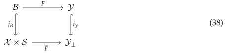
(Pullback characterization of the feasible domain). With the canonical inclusion, the square
is a pullback.
Proof.
The square commutes by restriction. Suppose Z carries maps and with . Then for every z, so the image of w lies in . There is consequently a unique map with ; commutativity forces . This is the pullback universal property. □
The inclusion is therefore monic. Its two restricted projections jointly and faithfully encode every feasible point, although may be a proper subobject of the full product.
Define the reduced joint projections and the physical-reality behavioral image by
and let be the corestriction of . The active-domain inclusion is
4.5. Nondegeneracy and the Exact Reduction Boundary
Corollary 1
(Exact activation and degenerate boundary). The following conditions are equivalent:
- (i)
- is record-forming nontrivial;
- (ii)
- ;
- (iii)
- ;
- (iv)
- there is no such that
- (v)
- there is no such that .
The following stronger conditions are also equivalent:
- (a)
- has a strong record-forming witness;
- (b)
- there exist with ;
- (c)
- there is no such that
Thus a weak witness already makes the formation-side factor nondegenerate in the complete totalized law. A strong witness makes it nondegenerate within the actual outcome law. The corresponding factorization obstructions record these two levels of observational nontriviality. Its state interpretation is established in the next section.
The proofs of the categorical construction are collected in the Appendix.
5. From Complete Formation Behavior to a State Object
5.1. A State Criterion Based on Complete Behavior
Terminality settles which reduced realization is canonical; it does not by itself explain why the second coordinate deserves the name state. That identity is fixed by the following behavioral criterion.
Definition 4
(Observation state). For a complete law , put . An element is an observation state precisely when the corestricted transpose
is bijective. Thus, every observation state is identified by one complete formation map, every realized complete formation map has an observation state, and no duplicate observation states remain. The definition is relative to the declared complete empirical domain on which the maps are compared.
Cartesian closure now verifies this criterion. The descended law transposes to , sending s to the complete map . The column quotient makes this transpose monic. After corestriction to its image , it is exactly the bijection . This monomorphism verifies the passage from behavior to the state criterion: one point of is one complete observation map, and no two points carry the same map.
The conclusion is independent of the labels used to implement the family. If is any complete implementation and exactly when , coequalizing this kernel pair produces a bijection onto . Any two behavior-minimal complete implementations are therefore uniquely isomorphic over the same map family; for , the isomorphism is .
B. Establishing the Observation State
By Definition V.1, distinct raw operations represent the same observation state precisely when their complete maps coincide. This identity is independent of the labels used to implement the family. Two raw operations represent different states precisely when their complete maps differ somewhere on within the declared complete empirical domain. A reference phase, detector configuration, array weight, sampling rule, cognitive condition, or protocol state occupies this axis exactly when it changes that map. Topology, probability, dynamics, and a specific physical realization may later enrich the object; its behavioral identity is already fixed by the universal construction.
With this behavior-minimal identity established, 1 says precisely that record-forming nontriviality leaves a nondegenerate formation-state coordinate in the canonical role-preserving interface. At this point the canonically descended law is
where is a complete row-behavior class and is the observation state just established. The first coordinate is therefore the behavioral image of what is observed under the declared observation family; it has not yet been identified with the antecedent physical state space. The second coordinate carries the observation state through which the record is formed. It is neither a spectator nor a consciousness, and it is more than the name of an instrument: two formation conditions define the same observation state exactly when they implement the same complete map on the first argument.
The distinction between behavioral and physical identity matters. A physical theory may distinguish states that the present family of observations does not resolve. Section 8 therefore returns to the antecedently certified physical state space and proves the exact compatibility condition under which Equation (44) lifts uniquely to a complete law on that physical state space paired with . Only after that lift do the two coordinates carry physical-state and observation-state identity simultaneously. The present section establishes the second identity without presupposing the first identification.
The order of the argument is essential to this conclusion. The fixed-input witness first supplies an empirical distinction. Kernel pairs then determine its complete behavioral identity, and coequalizers remove only labels that add no information. Unique descent produces the reduced law; the pullback recovers its feasible domain; terminality makes the result common to every active exact realization; and exponential transposition establishes the state criterion. Once , factorization through the first coordinate is impossible because at least two complete response maps genuinely remain.
Category theory follows the needs of this argument [25,26,27,28]; it does not supply the ontology. It removes arbitrary labels and expresses what every faithful representation must preserve. Because the proof is carried out in before probability, topology, dynamics, or operator algebra is chosen, the returned value may later be a distribution, channel, trajectory, correlation table, or another structured record. The construction is therefore not restricted to quantum measurement.
Deeper consequences demand richer structure. Fixing recovers the unary law . Introducing smoothness then yields independent tangent contributions from the two axes. In the quantum branch, coherent response, full circular phase, reversible mixing, composition, and consistent probability successively endow the canonical interface with additional structure. Complex qubit geometry, the Born trace pairing, the singlet cosine, and the Tsirelson bound emerge only along this enriched branch. Bell nonclassicality is consequently a precise consequence of this structure, not the source of the second axis.
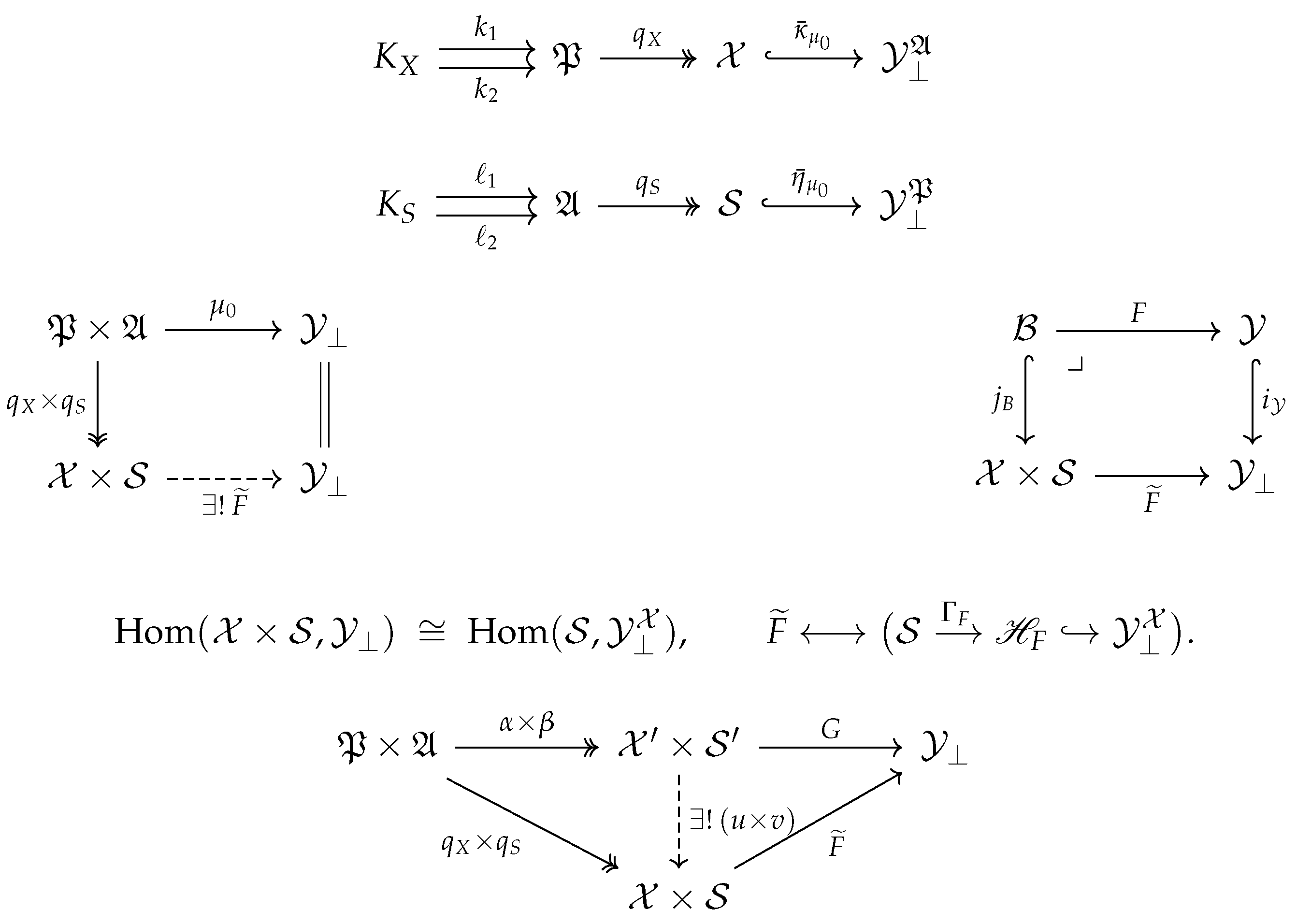
Figure 1.
The complete categorical chain. Kernel-pair coequalizers remove duplicate row and column labels; the middle diagrams give the unique descended law and its feasible pullback; exponential transposition establishes the observation-state criterion; and the final triangle expresses terminality among active typed exact realizations.
Figure 1.
The complete categorical chain. Kernel-pair coequalizers remove duplicate row and column labels; the middle diagrams give the unique descended law and its feasible pullback; exponential transposition establishes the observation-state criterion; and the final triangle expresses terminality among active typed exact realizations.
C. Irreducibility of the Observation State
Once is identified with complete observation maps, its irreducibility follows immediately.
Corollary 2
(No further factorwise quotient). If maps and satisfy
then q is injective. If q is also surjective, it is a bijection.
Proof.
If , Eq. (45) gives for every x. Injectivity of the exponential transpose, equivalently of , then gives . Thus q is injective, and an injective surjection is bijective. □
Distinct observation states may coincide at a particular x; behavioral minimality compares complete functions, not a single observation. This corollary holds for every factorwise map and preserves every distinction in the complete reduced second axis. The complementary fiberwise result for arbitrary exact encodings states that an enlarged coordinate retains every witnessed pair, whereas a smaller second factor cannot quotient without altering the complete observation law.
For a strong witness, set , and . Then while both points share the same physical reality coordinate . Applying this fiberwise argument to , keeps and distinct in every exact encoding that preserves this physical-reality projection. A weak witness yields the parallel non-hiding result for feasibility in the complete totalized law.
6. Hidden Coordinates, Decoders, and Label Erasure
An enlarged variable may conceal the notation of physical reality and observation conditions while retaining their behavioral distinction. Proposition V.2 preserves every witnessed pair. A global observation-state decoder exists precisely when this fiberwise preservation is coherent across the complete joint domain.
Use the active projections and from .
Definition 5
(Physical-reality-preserving exact extended encoding). A physical-reality-preserving exact extended encoding of F consists of a set E and maps
such that
The first equation preserves the declared physical-reality coordinate; the second preserves the actual outcome law. The decoder criterion below depends only on the kernel pair of ι relative to ; the maps and retain those two responsibilities.
Proposition 7
(Exact criterion for a global observation-state decoder). Let be a physical-reality-preserving exact extended encoding. Because , the following are equivalent:
- (i)
- there exists such that ;
- (ii)
When these conditions hold, d is uniquely determined on ; if ι is surjective, it is unique on all of E. Moreover,
and consequently ι is injective.
Proof.
If d exists and , applying d gives , proving the kernel-pair inclusion. Conversely, assume Equation (48) and define on . The inclusion makes well defined. Choose and extend to E by assigning outside . This constructs a decoder. Its values on the image are forced by , which proves the uniqueness statements. Equation (49) follows from the two coordinate laws; because is injective, so is . □
Corollary 3
(Primitive-table decoder criterion). Since , for an encoding , a decoder satisfying
exists if and only if
Proof.
If d exists, equality under e implies equality after applying d, hence the kernel-pair inclusion. Conversely, the inclusion makes well defined on . Extend to all of E by a fixed element of the nonempty set . □
physical-reality preservation and outcome fidelity constrain the first coordinate and recorded value, but do not by themselves imply Equation (51). For example, let , , , and
With , , and , one has and . Thus the encoding is physical-reality-preserving and outcome-faithful. The witness at cannot be hidden, but although the two columns define different elements of . Hence no global -decoder exists. The example isolates the additional cross-fiber coherence required of an arbitrary encoding.
The same coordinate may also be epistemically hidden: the observation state is retained in the complete law although its value is not appended to an observed record. For , define
and for define the nonempty actual response set
Proposition 8
(Observation-state label erasure). For the response sets in Equations (53) and (54):
- (i)
- record-forming nontriviality is equivalent to for at least one ;
- (ii)
- a strong witness is equivalent to for at least one ;
- (iii)
- a map satisfying exists if and only if every is a singleton, in which case h is unique.
Proof.
A primitive witness descends to two unequal values of at the same , and any two unequal values in one totalized response set lift to primitive representatives at a common preparation representative. This proves (i). The same argument restricted to values in proves (ii). For (iii), a factorization through makes F constant on every fiber. Conversely, if every is a singleton, define to be its unique element. Surjectivity of makes this definition unique and gives the required factorization. □
Erasing the observation-state label therefore gives a non-singleton response set at each physical-reality value that supports a strong witness.
A hidden state is therefore distinct from a duplicate state. In a downstream theory, observation-state labels may be fixed, recorded, unrecorded, treated statistically, or actively selected. A probability kernel on produces marginal laws, while the complete conditional maps retain the underlying state distinctions. Recovering those distinctions from unlabeled marginals is the corresponding downstream identifiability problem.
7. Invariance Under Empirical Refinement
A single physical experiment can be represented by tables of varying granularity. One description may split a single operation into multiple labeled steps, or rename the returned values, without altering the underlying physical facts. A canonical state interface must remain invariant under any such structural refinement that preserves the two roles. This requirement leads to the following notion of empirical cover.
Definition 6
(Role-preserving empirical cover). Let and be two operationally role-faithful complete tables. Arole-preserving empirical coverfrom to consists of surjections
such that , , and
Theorem 2
(Empirical-cover invariance). Let and be the reduced objects of the two tables in 6, with quotient maps . Then there are unique bijections
They satisfy
Let
Then the restricted laws obey
Record-forming witnesses, strong witnesses, weak witnesses, and the cardinality of are invariant under such covers.
Theorem 2 concerns the reduced behavioral interface. Antecedent physical identity is not reconstructed from a change of labels; it enters through the compatibility map developed in the next section.
Corollary 4
(Common-cover invariance). If two typed primitive records admit a common role-preserving empirical cover, their reduced dual-axis interfaces are isomorphic.
Proof.
Apply 2 to the two covering maps and compose one induced isomorphism with the inverse of the other. □
The theorem captures the full freedom of empirical presentation within each role: labels may be repeated or refined, and outcome names may change, while the reduced interface remains isomorphic. Typing carries the physical content that makes this invariance meaningful. Folding both inputs into and replacing the second by crosses that boundary when ; no surjection can preserve the formation role. Such a folding asks a different observational question. It cannot erase the second axis of the original experiment.
8. From Behavioral Identity to Physical Identity
The canonical physical-reality object records complete row behavior; it does not define physical identity. The antecedent space may retain distinctions that the declared observation family cannot resolve. The next step is therefore a change from behavioral image back to physical identity. In Set, the surjection is the coequalizer of its kernel pair. Compatibility says that every r-identified pair has the same complete row, or equivalently . The universal property of r must then produce , while constancy in the second argument produces a law on . The proposition states this factorization and shows that the observation transpose remains monic after the lift.
Proposition 9
(Behavioral and physically refined first-axis interfaces). Let , let , and let be the canonical two-sided reduced law. Suppose an antecedent physical theory supplies a surjection satisfying
Then: (i) there is a unique surjection such that ; (ii) there is a unique map satisfying
(iii) the physically refined feasible domain and outcome law are
With the canonical inclusion , the defining square is a pullback; (iv) the formation-side transpose is injective; (v) κ is bijective if and only if implies .
Thus is the behavior-minimal first axis, whereas may retain distinctions not resolved by the present observation family. The symmetric terminal property belongs to the pure two-sided behavioral realization; formation-side minimality and observation-state identity remain valid in the physically refined branch.
Corollary 5
(Physical-axis factorization boundary). Under the hypotheses of proposition VIII.1, the following are equivalent: (i) is record-forming nontrivial; (ii) ; (iii) there is no map for which
Proof.
The equivalence of (i) and (ii) is corollary IV.6. If the factorization in (iii) existed, every slice of would equal ; the injective formation-side transpose in proposition VIII.1(iv) would then force to be a singleton. Conversely, if , define . □
The map has a precise meaning. It records the resolving power of the declared observation family: two physically distinct states may have the same complete row in the present table. Such a coincidence makes the behavioral image coarser; it does not identify the physical states and cannot delete the physical axis. Physical identity is fixed by the antecedent theory, whereas records only the distinctions visible through .
When the preparation labels are related to an antecedent physical state space by a surjection , Eq. (62) is the exact bridge from the primitive physical-reality identity to the descended physical law.
IX. The PODA Axiom
The row-column reduction produces the canonical typed behavioral structure, while the antecedent map remains fixed. Proposition VIII.1 shows that compatibility uniquely factors the behavioral map through this prior identity, , and thereby lifts the complete law to . The observation-state object is unchanged, because it is already the behavior-minimal realization of the complete observation-map family.
The acronym PODA stands for Physical-Observation Dual-Axis. It names the ordered pair of state responsibilities retained in the anchored interface: physical state on the first axis and observation-formation state on the second. The actual-output object is not a third state axis, and no human observer is implied.
Axiom 3
(PODA Axiom). A complete PODA model is a physical–observation dual-axis interface consisting of nonempty typed sets and , an actual-output set , a fresh symbol with , and maps
satisfying the following conditions.
- (P1)
- carries the physical-state identity supplied by an antecedent physical theory, while carries the observation-condition state (i.e., the observation state). They are distinct sorts even if their underlying carrier sets happen to be equal.
- (P2)
- The coordinate map is monic. Thus the two projections jointly determine every admissible joint state, but no equality is assumed.
- (P3)
- Writing for the canonical inclusion, the square formed by and is a pullback. Equivalently,
- (P4)
-
The exponential transposeis monic. Its image is the realized family of complete observation maps, and the corestriction of to that image is therefore a bijection. Thus the observation condition (observation state) is complete for the map family it realizes and contains no duplicate complete behaviors.
In Set, (P2) follows from (P3), because a pullback of a monomorphism is monic; it is displayed separately to expose the joint-coordinate semantics. Condition (P3) uniquely fixes the totalization:
The first branch is well defined by (P2). Here an “axis” is a typed state role with its own projection. It may be multidimensional, nonlinear, interacting, and feasible only on a proper joint subdomain.
Proposition VIII.1 proves that every compatible physically refined branch of the canonical reduction satisfies (P1)–(P4). Physical identity is carried by the antecedent interface, while behavioral reduction determines the canonical observation axis. Their lawful conjunction is the culmination of the present derivation and the structural axiom from which downstream PODA models begin.
The construction follows a strict order of dependence:
Physical identity is established on the first line, prior to any categorical reduction. The complete record table then sheds its behavioral redundancies, giving rise to the minimal observation object. Their compatible law is the third line. The PODA Axiom designates this invariant conjunction. When record formation is nontrivial, the second axis is nondegenerate and the complete law cannot factor through the physical projection; a strong witness carries the same conclusion into the actual-outcome law. The physical axis is rendered non-deletable by antecedent identity, while the observation axis is rendered non-deletable by witnessed difference and behavioral minimality.
The derivation is complete at this point, before any discipline-specific structure has entered. The physical–observation dual-axis form is therefore not a discipline-specific hypothesis, but a general theory of fact formation. Specific sciences emerge only downstream, when the value object and its associated interface are endowed with a specific algebraic structure. Probability distributions, channels, trajectories, correlations, and structured records all become particular value objects within their respective downstream theories. The discussion below first draws out the general physical meaning of the derived interface, and then follows one especially rich branch into quantum mechanics.
Table 2.
Logical division between the generating theorem and the reusable axiom interface.
| Question | Generating theorem | Axiom interface |
|---|---|---|
| Where do the states come from? | Quotient complete behavior and preserve the antecedent physical interface | Receive the already established and |
| Is every fact preserved? | Prove the master factorization entry by entry | Use the resulting admissible output law |
| Why two coordinates? | Exclude first-projection factorization by nontriviality, then use the product to pair the surviving roles | Retain the two state responsibilities explicitly |
| Why call the second coordinate a state? | Use exponential transposition, image factorization, and terminality to establish complete behavioral identity | Require the behavior transpose to be monic |
| Logical status | Structural conclusion at the foundational level | Reusable starting point for enriched theories |
9. Kernel Pairs, Observational Equivalence, and Conditional Identifiability
The dual-axis structure is now established. The next question is not whether the two states exist, but which of them can be recovered from a record under a specified condition. This distinction is essential: behavioral minimality defines state identity by complete response, whereas identifiability asks what one particular law can distinguish on its feasible domain.
For Section 10–14, fix a physically anchored model of Axiom 3 and lighten the notation by writing
Thus denotes the antecedent physical state carrier throughout these sections, rather than the coarser row-behavior image used in the generating construction. The observation carrier is unchanged by the physical lift. Let and denote the active images. For an arbitrary map , its kernel pair is the pullback
Applied to the dual-axis law, this gives
The first two relations express equality of the two state coordinates; the third expresses equality of the resulting record. Their meanings are different and cannot be interchanged. Since the paired projection is monic,
where .
Definition 7
(Observational equivalence). Two admissible joint states are observationally equivalent under F, written , when . Their equivalence class is .
The quotient map is the coequalizer of . If is the surjective part of the image factorization of F, then there is a unique bijection
The observational quotient is therefore not an arbitrary binning of results; it is the finest distinction among joint states that the present output law can support.
9.1. Fixed-State Slices as Pullbacks Along Points
For define
and for define
Categorically, is the pullback of along the point , and is the pullback of along . Holding one axis fixed is thus a canonical base change, not an informal convention.
Definition 8
(Conditional physical-state identifiability). For fixed s, the physical state is globally identifiable on that observation slice when is monic, hence injective in . A particular x is identifiable at conditional on known s when .
Definition 9
(Conditional observation-state identifiability). For fixed x, the observation state is globally identifiable on that physical slice when is monic. A particular s is identifiable at conditional on known x when .
Proposition 10
(Kernel-pair criterion for conditional identifiability). Observation states are identifiable on every fixed-physical-state slice if and only if
Physical states are identifiable on every fixed-observation-state slice if and only if
Proof.
The left-hand side of Eq. (83) contains exactly the pairs with equal physical coordinate and equal output. It reduces to the diagonal exactly when every is injective. The second statement is the dual argument. □
10. Identifiability without the Label of the Other State
Conditional identifiability assumes that the other coordinate is known. If that label is absent, changes on the two axes can imitate or cancel one another. For define
These sets list, respectively, the admissible joint states, physical states, and observation states capable of producing y.
Definition 10
(Label-free physical-state identifiability). The physical state is identifiable from the output without an observation-state label when for every .
Definition 11
(Label-free observation-state identifiability). The observation state is identifiable from the output without a physical-state label when for every .
Definition 12
(Joint identifiability). The joint state is globally identifiable when is monic, equivalently when every nonempty is a singleton.
Let and be the corestricted active projections.
Theorem 4
(Descent criterion for label-free identifiability). Let be the regular epimorphic part of the image factorization of F. Then:
- (i)
- the physical state is label-free identifiable if and only if , equivalently if and only if there is a unique decoder satisfying
- (ii)
- the observation state is label-free identifiable if and only if , equivalently if and only if there is a unique decoder satisfying
- (iii)
- the joint state is identifiable if and only if , equivalently if and only if F is monic.
If both marginal label-free conditions hold, then the joint state is identifiable.
Proof.
The first kernel-pair inclusion says that every pair merged by is also merged by . The universal property of the coequalizer of the kernel pair is therefore exactly the unique descent of through . Fiber by fiber, this is the singleton condition for . The second assertion is dual. The third is the kernel-pair criterion for a monomorphism. If the first two conditions hold simultaneously, then
the reverse inclusion always holds. □
The theorem states precisely what it means to recover either axis from an output. It does not assume that F possesses an inverse on all of ; it requires the corresponding coordinate projection to be constant on each observational fiber and hence to descend uniquely through the output quotient.
10.1. Response-Set Separation and Cross-Axis Ambiguity
Define
Proposition 11
(Response-set separation). The physical state is label-free identifiable if and only if . The observation state is label-free identifiable if and only if .
Proof.
If the response sets of two different states intersect, one output has two sources on that axis; the converse is immediate. □
The relation
is reflexive and symmetric but need not be transitive.
Counterexample 5
(Projected confusability need not be transitive). Let , , and . Then and , but . An equivalence relation on joint states may therefore project to a mere confusability relation on one axis; no quotient is legitimate without a separate proof of transitivity.
10.2. Two-Sided Conditional Identifiability Does Not Imply Joint Identifiability
Counterexample 6
(Exclusive-or law). Let , , and . For every fixed s, the map is bijective, and for every fixed x, the map is also bijective. Nevertheless, and , so F is not monic.
The example isolates the central two-axis ambiguity. When the other axis is known, either state may be recovered exactly; when it is unknown, changes of the two states can cancel. Conditional and joint identifiability are therefore different mathematical claims.
11. Same-Source Pullbacks and the Lawful Starting Point of Transport
11.1. The Canonical Domain of Fixed-First-State Comparison
Definition 13
(Same-source pair). Two admissible joint states form a same-source pair when .
Here “same source” means only equality of the first-state projection. Under the physically anchored interface it means equality of the inherited physical state; it does not additionally assert simultaneity, common noise, or causal identity. All ordered same-source pairs form the pullback
Its universal square is
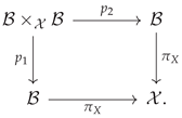
This pullback is the maximal canonical comparison domain on which the first state remains fixed while the observation state varies; no hand-chosen pairing rule is required.
Proposition 12
(Same-source ambiguity). The nontrivial pairs of observation states that remain indistinguishable at a fixed physical state are exactly
Proof.
Every pair in this set has equal first coordinate and equal output but is not the same joint state; the two points can therefore differ only on the observation coordinate. The converse follows directly from the definitions. □
At the set level, a same-source pair , supplies only and . Their equality means that the two observation states are indistinguishable on this slice; their inequality makes the change visible. Since is still only a set, no difference, ratio, phase displacement, or group element is yet canonical.
11.2. Fixed Observation State and General Joint Variation
Dually, the comparison domain at fixed observation state is
Any two admissible observations may differ only in physical state, only in observation state, or in both. A joint change need not decompose into the first two kinds because the required intermediate cross-combinations may not belong to .
Counterexample 7
(A nonrectangular feasible domain). Let , , and . The change from to cannot be decomposed through either or because neither intermediate point is feasible.
Even when both cross-points exist, a decomposition of into a pure physical contribution and a pure observation contribution requires additive, group, or geometric structure on the output; it is not a theorem of sets.
11.3. Why Transport Begins on the Same-Source Pullback
The dual-axis theorem does not itself postulate a transport equation. It constructs the domain on which such a question can first be asked correctly: . When responses are subsequently enriched by nonzero complex amplitudes, a group action, a bundle, or a connection, phase differences, group displacements, and consistent transport can be defined on same-source pairs. Identifiability answers whether states can be distinguished; transport answers how two representations are compared. Neither replaces the other. The two state objects, the feasible joint domain, and the same-source pullback are therefore the categorical foundation of observation geometry; phase transport begins here and is never used retroactively to prove the dual-axis structure.
11.4. Observation-Axis Prediction and Same-Source Discovery
The same-source pullback is not only a domain of comparison; it is a predictive domain. For each physical state x, define the feasible observation fiber and its response profile by
The image is the complete spectrum of facts accessible from the same physical source through the declared family of observation states. Once has been determined on a lawfully generating family, it predicts the record for every further feasible s; conversely, systematic variation of s at fixed x exposes symmetries, degeneracies, critical points, and previously unresolved response sectors that are invisible on any one fixed slice.
Proposition 13
(Canonical same-source prediction). The family of profiles is invariant under every replacement of raw preparation and formation labels that preserves the complete record law and the certified physical-reality identity. Hence any prediction expressed through the fibers, images, or equality relations of belongs to the canonical dual-axis realization rather than to a choice of experimental labels.
Proof.
Behavior-preserving relabelings descend uniquely through the two kernel-pair coequalizers. The descended law is unique, and the terminality theorem gives the unique compatible isomorphism between behavior-minimal realizations. Restricting that isomorphism to the fiber over x carries to the corresponding profile without changing its values, fibers, or image. □
When the output is linear or probabilistic and the joint law is smooth, the finite and infinitesimal same-source responses are
A nonzero coherent response makes phase comparison possible. Crucially, this transport unfolds precisely on the observation axis. Since the observation state s varies along the same-source domain, we must specify how the coherent response is transported from one observation condition to another within the observation space. In the simplest scalar (single-component) case, the observation map determines a complex response. The requirement of a consistent phase comparison on this axis then forces the normalized phase to define a connection one-form, yielding the original Phase Transport Fundamental Equation (PTFE) [41] on the observation space. The finite endpoint factor is precisely the solution of this equation along the observation path. While this scalar construction provides the foundational intuition for phase transport, the following statement extends it to a Hermitian response space. The distinction matters: scalar reference conversion and transport of a multicomponent ray do not, in general, have the same curvature or endpoint content.
Theorem 8
(Phase transport and its coherent extension). Fix a physical state x. Let the feasible observation fiber be a smooth manifold, let V be a finite-dimensional complex Hermitian response space, and let
be a smooth coherent response along a piecewise path . The Hermitian geometry fixes the canonical connection, and its pullback defines a common-phase transport that is the identity on a constant path, reverses under path reversal, and composes under path concatenation. On the phase bundle , let be the projection, let ζ denote the fiber coordinate, and let be the lifted path:
The representative
In the one-dimensional scalar specialization , for endpoints and in a nonzero chart,
Proof.
Normalization gives , so is purely imaginary and is a real one-form. The horizontality equation pulls back to , which is exactly Eq. (); integration gives Eq. (). Substitution in Eq. (103) cancels the vertical component and proves horizontality. Line integrals add under path concatenation, change sign under reversal, and vanish on constant paths, so the corresponding transport factors have the stated composition laws. When , write locally. Then , and Eq. (104) follows directly. □
The response, phase one-form, compatible connection, and horizontal lifting equation enter in that order. Here is a one-form on the observation fiber; is the principal connection on the phase bundle. For a scalar response, compatibility with its phase differential fixes the connection uniquely, and Eq. (104) is its finite same-source solution. For a multicomponent response, the Hermitian geometry supplies the indicated common-phase connection, but the horizontal representative can still move as a ray. Its inverse phase factor therefore need not recover an entire reference vector. Physical dynamics evolves the first state; this construction compares responses along a prescribed path of observation states at fixed physical input.
The normalized form of is essential. The numerator scales with response intensity; division by isolates its vertical phase transport. In one complex dimension this reduces to . On a general bundle the local forms transform as and the endpoint factors transform covariantly. For a globally nonzero scalar response, is closed, so its compatible connection is flat even when a real phase lift has nonzero winding. If a closed loop lies in a regular chart, then
For a globally defined scalar response the loop integral records its winding around excluded zeros, while its exponentiated closed-loop factor is unity. For a multidimensional projective response, or for a nontrivial bundle, curvature and bundle topology can produce nontrivial holonomy. The path may not cross a zero, because normalization, phase, and their transport cease to be defined there.
Zeros of , its rank changes, invariant singular values, and the holonomy of closed observation-state loops are direct targets of experiment. They constitute an observation-axis spectroscopy: the physical source is held fixed, while the geometry of fact formation is scanned. This opens a general route to discovery. A structure hidden by one observation state can become visible under another, and a nonzero mixed curvature can reveal that physical evolution and observation transport do not commute.
The familiar theories give immediate realizations. For a quantum state and a smoothly varied POVM element ,
so scanning the observation axis reveals coherences and correlation directions that a fixed basis cannot see; the Horodecki maximum is exactly such an optimization over observation states. In relativity, a fixed four-momentum gives the observer-dependent energy as the timelike observation state u varies. In gauge physics, closed changes of internal reference or probe path yield the holonomy
whose infinitesimal content is curvature. Quantum tomography, relativistic frame comparison, and gauge holonomy are therefore not isolated techniques; they are three expressions of the same principle of discovery from a physically identical source along a varied observation axis.
The same principle converts directly into a design law for quantum technology. Let be a figure of merit for a complete feasible response, bounded above on every observation fiber. Fixed-source observation design and full dual-axis co-design are, respectively,
The first expression isolates the performance available from the observation axis while the physical source is held fixed; the second permits the two axes to be engineered together. In quantum communication the physical coordinate contains the prepared signal ensemble, any encoding that changes that preparation, the channel, and the entanglement resource. The observation coordinate contains the receiver phase reference, detection basis, complete instrument, adaptive measurement state, and decoding measurement. Secret-key rate and fidelity can therefore be optimized first along the observation fiber of one physical channel and then over the complete source–observation design. In quantum computing the physical coordinate contains the register, gates, noise process, and controlled evolution, while the observation coordinate contains calibration reference, readout basis, adaptive measurement, and feedback state. Gate fidelity, success probability, and logical accuracy are then objectives on the same admissible joint domain. The observation axis is thus an objective engineering dimension. It turns measurement from a terminal readout into a controllable part of computation and communication, and it converts same-source comparison into a systematic method for finding hidden coherence, correlation directions, and order-dependent control effects.
12. Structural Domain and Pathways to Enrichment
The empirical witness and the categorical construction contribute different parts of the result. A complete record supplies the fixed-physical-reality difference. Kernel pairs, coequalizers, unique descent, products, pullbacks, and image factorizations then preserve every such difference while removing duplicate encodings. Every faithful typed realization therefore reaches the same behavior-minimal form.
Formal unarity and structural unarity are distinct. The pair may always be renamed as one symbol e, but a faithful encoding still carries the projection that expresses comparisons at fixed physical-reality identity. When the kernel criterion of 7 holds, it also carries the global observation-state decoder. A coordinate disappears structurally only when the complete law descends through the complementary projection.
Each universal construction fixes one responsibility. The product pairs the two typed maps without imposing orthogonality, independence, or dynamical decoupling. The feasible domain may occupy a proper subobject of that product. Behavioral minimality compares complete maps, whereas pointwise identifiability compares one slice. The antecedent interface preserves physical identity even when the current observation family resolves a coarser row behavior. Observational equivalence is an equivalence relation on the joint domain, while its projection onto one axis may be a nontransitive confusability relation. The same-source pullback fixes equality of the first state and thereby supplies the domain on which later algebraic comparison, phase, and transport can be defined.
The value object may be a scalar outcome, a complete probability distribution, a stochastic kernel, a channel, or a structured trajectory. Equality in that value object defines the two behavioral kernel pairs, after which quotienting, descent, terminality, product pairing, pullback feasibility, and exponential transposition proceed unchanged. Statistical sufficiency, information loss, Fisher geometry, and local observability enter as further structure on the canonical interface.
13. Physical and Philosophical Consequences
13.1. From Nontrivial Observation to Relational Objectivity
The fixed-state difference with which the derivation began now has a canonical home. It is the separation of at least two complete observation maps in , witnessed at one value of the physical reality. The compatible lift carriesthat separation to the antecedent physical space itself. A fact is thereforeformed at : the physical state supplies what enters observation, and theobservation state supplies the objective condition under which it becomes a record.
This is the foundational break with single-axis physics. Observation is placed inside objective physical reality as a state-bearing structure with its own identity, variations, and lawful couplings. The object of fundamental theory is consequently enlarged from the state of a system to the ordered triple consisting of physical state, observation state, and the fact-forming law that joins them.
The familiar unary form appears here as a boundary case, not as the premise of the construction. Corollary VIII.2 proves that an activated observation admits no map for which
A physical state remains a fully meaningful state of the world. What it does not carry, once observation is nontrivial, is one record valid independently of the state of observation. Omitting s leaves the family , not a single value. The obstruction to unary factorization is the mathematical shadow of the positive structure already found: distinct observation states realize distinct complete maps.
The theorem changes the ontology of the record. A fact is not an unknown unary attribute waiting inside x; its mathematical bearer is the objective relation . Its two arguments are irreducible for different reasons. Antecedent theory fixes physical identity, including distinctions finer than the present observation family can resolve. Complete formation behavior fixes observation identity. The original witness keeps this second responsibility from being absorbed into the physical projection. Both states, and the law that joins them, belong to a complete account of the fact.
Dual-axis irreducibility reaches deeper than an observation–disturbance model, which lets an operation change an object and then reads the changed state. The dual-axis theorem preserves the identity held fixed beneath that process: every exact enlarged encoding that preserves it must also preserve the witnessed variation within its fiber. Proposition VI.2 captures the distinction. Writing as one longer coordinate may hide the typography of the second axis, but it leaves its state responsibility untouched.
The resulting ontology is relational objectivity. The two state roles, their admissible joint domain, and their joining law are fixed independently of any individual’s knowledge. Different values of s can form different facts at the same x without making either fact subjective. An apparatus, reference frame, environment, or another physical system may realize the observation state; none defines it by name. Its identity is the complete behavior that survives canonical reduction.
The human observer thereby leaves the foundations. A person may choose or learn an observation state, but neither consciousness nor agency defines . Physical state and observation state are equally objective in their different roles, and the fact relating them belongs to their joint law. Theorem VII. 2 gives this conclusion its invariant content: every active typed exact realization contains the same behavior-minimal second object, up to unique isomorphism.
13.2. Classical Laws as Exact Fixed-Axis Sections
Choose . The inclusion , , induces
The unary form familiar from fixed-context classical modeling is therefore an exact section of the dual-axis law. Its enormous success reflects stable observation states: calibration, symmetry, scale separation, and experimental control keep effectively fixed. What appeared to be the universal form of a physical law is the fixed-axis regime of a larger law.
When all complete maps coincide, and the unary description is globally sufficient. A strong witness separates two such maps and opens the genuinely dual-axis regime. The fixed-observation form of classical modeling is therefore the degenerate boundary of PODA Theory.
With smooth structure, a joint path yields
The two tangent contributions remain distinct even when F is nonlinear and nonseparable. The first term is change of the observed state; the second is change of the state of observation formation. In coherent complex models the latter may acquire a connection and a phase-transport law. Stochastic kernels, control actions, channels, biological response functions, and cognitive transitions are different enrichments of the same two state responsibilities.
The same fixed-section statement extends from outcome laws to geometric transport. This yields the common kinematic theorem behind the different physical realizations.
Theorem 9
(Enriched dual-axis realization and exact sector recovery). Let be a smooth regular sector of a theory T, equipped with the local tangent splitting
such that the tangent image of every defined fixed-observation section lies in . Let be a smooth structure map and let carry a principal connection with curvature . Then the pullback bundle carries the connection and curvature . In every local trivialization its connection form has the unique decomposition
If is a fixed-observation section, then
Consequently the fixed-observation theory is recovered exactly as the pullback along , whereas transport on the full domain contains physical, observation, and mixed curvature sectors. Equivariance, parallel transport, and holonomy are inherited functorially from .
Proof.
Existence of and of the pulled-back connection follows from the universal property of the bundle pullback. Naturality of exterior differentiation and of the Lie bracket gives . The projectors in Eq. (113) resolve every tangent vector uniquely, which gives Eq. (114). Along every tangent vector lies in ; hence , and every curvature term containing an argument vanishes. This proves Eq. (115). Functoriality of pullback preserves equivariance and parallel transport, and therefore preserves holonomy up to conjugation at the chosen initial frame. □
The theorem does more than place established theories side by side. It derives their common kinematic form from the dual-axis domain and proves that a familiar fixed-observation theory is an exact sector, not a rival ontology. The characteristic symmetry group, invariant tensors, and action then select the physical realization and its dynamics.
Relativity and gauge theory enter through this interface with their established geometric data intact. In the relativistic realization, carries the Levi–Civita connection (or the spin connection after a spin lift) and Riemann curvature [53]. A passive change of coordinates or tetrad components is representational and is quotiented away; a change of an actual observer’s four-velocity, clocks, rods, orientation, or local orthonormal frame belongs to the observation role whenever it changes the recorded energy, frequency, or spatial decomposition. In the gauge realization, carries the gauge connection and curvature [54,55]. A mere change of local section is again representational, whereas a change of probe path, coupling protocol, internal reference apparatus, or boundary condition can be a genuine change of observation state. The common local law
separates local description from invariant content; curvature invariants and holonomy class functions supply representation-independent readouts.
Table 3.
Major physical theories as realizations of one dual-axis architecture. The observation coordinate is objective: it denotes the state of frame, reference, coupling, or complete test through which a fact is formed, never the consciousness of an observer.
Table 3.
Major physical theories as realizations of one dual-axis architecture. The observation coordinate is objective: it denotes the state of frame, reference, coupling, or complete test through which a fact is formed, never the consciousness of an observer.
| Theory | Physical axis | Observation enrichment | Law recovered at the interface |
|---|---|---|---|
| Classical mechanics | Phase-space state | Fixed rods, clocks, frame, and calibration | Hamiltonian or Newtonian law as an exact fixed-observation section |
| Relativity | Matter and spacetime state | Timelike frame, tetrad, clocks, and orientation | Lorentz-covariant records and frame transport; the fixed-frame pullback recovers the usual local description |
| Gauge field theory | Matter fields and gauge-field state | Internal reference, probe path, coupling protocol, and boundary condition | Covariant derivative, curvature, and holonomy on the joint domain; a fixed-reference section recovers the ordinary gauge-sector law |
| Quantum theory | Density operator or projective state | Complete POVM or instrument, including phase reference and context | Born probability, outcome-conditioned transition, tensor composition, and Bell correlations |
13.3. Mathematics Selected by Observation Structure
Mathematics enters PODA Theory in a precise role. It is the instrument with which physical structure is represented and proved, rather than the object discovered. Once the empirically given architecture and symmetries of observation are fixed, however, their invariants select which instruments can represent them faithfully. Mathematics remains a tool, while the structure to be expressed can make the form of that tool necessary.
The categorical theorem first supplies the behavior-minimal observation axis over the certified physical role. The quantum branch then adds empirically specified structures in a strict order. Standard classification, projective geometry, and probability theorems organize the successive implications
Each line uses the structure introduced at that stage. Frobenius classification makes full circular phase select the scalar algebra before a complex vector space is available [39]. The invariant Hermitian form and ray quotient then generate the Hopf–Bloch sphere [40]; after an orthonormal choice of coordinates, the Pauli operators span the traceless part of . Independent composition then raises two binary response spaces to . Complete contexts and response-filter identity glue the probabilities of separate tests into one positive orthogonally additive measure on the full projector lattice. Only at that point does Gleason’s theorem [42,43] fix the trace form; composite marginal consistency returns it to each binary factor. Complex numbers, Bloch geometry, Pauli coordinates, event measures, and Born probability therefore appear in the order in which the observation structure requires them.
This reverses the usual explanatory direction. The question is no longer why physics happened to borrow complex numbers, projective Hilbert space, and the Pauli algebra. It is which invariant requirements on coherent observation make those structures unavoidable. Different scientific domains may select different enrichments, but the mathematics is constrained by the architecture and symmetries of their observation states. Physical theory does not simply choose a mathematical language; sufficiently strong observational structure selects its own natural language.
This selection principle extends beyond the quantum branch. For , let a smooth structure map send a joint physical–observation state to the intrinsic base used by the corresponding mature theory, and let carry its principal connection [56]. The pullback transports the entire principal-bundle geometry to the fact-formation domain. Parallel transport along a path in the joint domain is precisely the pullback of transport along ; closed-loop holonomy agrees up to the usual conjugation associated with the initial frame. Relativity takes and , the pure-state quantum sector takes and , and gauge theory takes and . They consequently share three structural layers: two-role fact formation, covariant representation under a group action, and geometric transport by connection, curvature, and holonomy. Their state spaces, structure groups, actions, couplings, and empirical content remain those of the individual physical theories.
The joint geometry also contains a component absent from a fixed-axis description. On a local product chart, write
For covariant derivatives along commuting coordinate directions of that local product chart, in any representation,
For general vector fields , the corresponding identity is . Thus is the infinitesimal obstruction to exchanging physical evolution with observation-state transport. The vanishing case recovers local commutation to first order in enclosed area; a nonzero mixed component records a genuine order-dependent coupling. This is the precise geometric interface through which relativistic frame transport and internal gauge transport can be incorporated without identifying either one with observation geometry itself.
14. Quantum Enrichment: from Coherent Response to Born Probability
The categorical construction fixes the two state responsibilities and the complete law that joins them. At the level of sets it leaves a further question open: how do unresolved alternatives combine inside a binary observation, how is phase transported, and which transformations preserve the identity of a response? The quantum branch begins when coherent superposition makes these operations physical. Its mathematics is introduced in the order in which those questions arise; none of the following enrichment conditions is needed for the general dual-axis theorem.
The following diagram records the route ahead without replacing its intermediate arguments. Probability does not enter at the beginning: it is introduced only after coherent response has acquired a scalar field, reversible mixing has fixed projective event geometry, and independent composition has created the domain on which event probabilities can be glued across complete contexts.
Figure 2.
The quantum representation is built on the already established dual-axis interface. Full scalar phase selects the local scalar geometry; composition creates the domain on which projective completeness and additive probability become rigid; the Born interface then joins both axes in the correlation law.
Figure 2.
The quantum representation is built on the already established dual-axis interface. Full scalar phase selects the local scalar geometry; composition creates the domain on which projective completeness and additive probability become rigid; the Born interface then joins both axes in the correlation law.
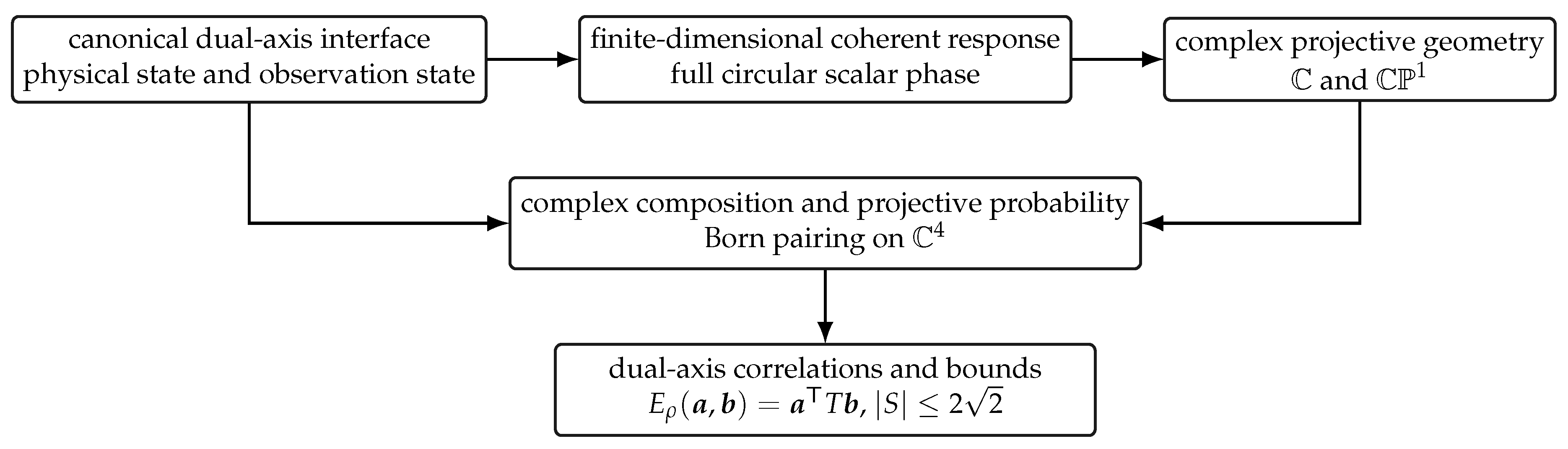
15. Full Circular Phase and the Selection of Complex Scalars
Let denote two perfectly distinguishable primitive response channels. A coherent alternative has the form
Addition represents alternatives that remain unresolved, while sequential response requires a compatible multiplication of coefficients. To identify the finite-dimensional scalar geometries compatible with these operations, we impose the following algebraic closure condition.
Axiom 10
(Coherent binary response). The coefficients in Eq. (120) form a finite-dimensional unital associative real division algebra , and the binary response space is the free rank-two left module
Thus are linearly independent and every coefficient pair in represents an allowed response vector. Addition combines unresolved mutually exclusive alternatives, multiplication combines sequential responses, and multiplication distributes over addition. The algebra carries a continuous multiplicative modulus
Coherence supplies possible scalar algebras but does not yet select one. Continuous phase transport supplies the missing invariant. It must specify the whole reversible scalar freedom: a circle merely embedded in a larger phase group would leave the algebra undetermined.
Axiom 11
(Full circular scalar phase). Every norm-one scalar, and only such a scalar, is a reversible scalar phase. The full phase group
is topologically isomorphic to the circle group . Phase transports along concatenated paths multiply in , and no additional scalar phase degrees of freedom exist.
The phase condition now acts on the candidate class supplied by coherent response.
Lemma 1
(Multiplicative-modulus lemma). Let be isomorphic to , , or , and let N satisfy Eq. (122). There is an such that
where is the canonical Euclidean norm. The three full norm-one groups are therefore
respectively.
Proof.
On the central positive scalars , N is a continuous homomorphism of the multiplicative group into itself, and hence . Continuity at zero together with gives . Every nonzero element has a polar decomposition , where and u belongs to the canonical compact unit group. The image of that compact group under N is a compact subgroup of and is therefore . Thus , which gives Eq. (125). □
Theorem 12
(Complex-scalar selection). The coherent-response and full-circular-phase axioms imply
uniquely up to real-algebra isomorphism.
Proof.
Frobenius’ theorem leaves precisely the three finite-dimensional unital associative real division algebras , , and [39]. By 1, their full phase groups are, respectively, the discrete two-element group, the circle, and the three-dimensional non-Abelian group . Only has the full phase group required by Axiom 11. □
Within the finite-dimensional associative division-algebra class, the complex field has therefore not been chosen as a convenient coordinate system. The coherent-response axiom poses a division-algebra question, and the exhaustive topology of reversible scalar phase answers it. The real field has too little phase; the quaternions have a larger non-Abelian phase group; the requirement that the full phase group be a circle fixes the scalar algebra at . The imaginary unit records the tangent direction of continuous phase transport, while complex multiplication records its composition. The exponent in the multiplicative modulus remains undetermined at this stage. Here N identifies equal-modulus phase orbits; it is not yet a probability. The quadratic probability law appears only after event identity has been carried through composite contexts and the resulting projector measure has acquired its trace representation.
16. Reversible Mixing and Binary Projective Geometry
Complex scalars still leave an arbitrary choice of coordinates on the two-channel response space. Reversible mixing removes that arbitrariness and produces the metric needed to speak of normalized response directions. On channels , write the elementary reversible mixer as
Axiom 13
(Complete ray identity). The pure response-event space is exactly : every nonzero vector represents a realizable pure event, and two vectors represent the same event precisely when they belong to the same complex ray. A complete test is carried to another realizable complete test by every reversible transformation. Orthogonality and normalized representatives will be fixed by the invariant metric below.
Axiom 14
(Reversible mixing). Reversible transformations of a finite response block are complex linear, and their closure is a compact group . The group acts irreducibly on each irreducible response block and contains independent channel phases, channel permutations, and, for every allowed channel pair and every , the Givens mixers of Eq. (127). The primitive ordered channel frame is a realizable complete test.
Lemma 2
(Invariant Hermitian metric). Every irreducible binary response block carries a positive Hermitian form h preserved by all reversible mixers. The form is unique up to an overall positive factor. After normalization of the primitive channels,
Proof.
Choose any positive Hermitian form and average it over with normalized Haar measure:
The average remains positive and becomes -invariant. If and are two invariant forms, write with T positive and -self-adjoint. Invariance makes T commute with ; complex irreducibility and Schur’s lemma give with . Independent phases make and orthogonal, and their permutation gives equal length. Normalization yields Eq. (128). □
Theorem 15
(Binary projective geometry). Normalized pure binary response events constitute
Every ordered orthogonal ray pair constitutes a reversible image of the primitive channel frame, thereby yielding a realizable labeled two-outcome projective test. Consequently, these tests are parameterized by a single point on , with the two event components represented by antipodal points.
Proof.
Invoking axiom XV.1 and theorem XV.4 establishes . Complete ray identity ensures that all its nonzero rays are physically realizable. The invariant Hermitian form then guarantees that every nonzero ray intersects the unit sphere in exactly one common-phase orbit, naturally yielding . On the binary block, the Givens family, independent phases, and channel permutations together generate . Consequently, the covariance of realizable tests carries the primitive ordered frame to every ordered orthonormal frame.
For , the associated Bloch vector is defined by
A direct algebraic verification reveals that , while n remains invariant under multiplication by any nonzero complex scalar. Conversely, any point
is mapped to the unique complex ray
This establishes the Hopf–Bloch diffeomorphism [40].
The phase orbit and the Bloch sphere are therefore revealed as the fiber and base of the same Hopf bundle,
The invariant Hermitian geometry admits the canonical Hopf connection on . Under , it transforms as , while the closed-loop holonomy remains invariant. This corresponds exactly to the realization of the phase-transport connection in Eq. (100): pulling the Hopf connection back along a smooth same-source response yields . Its horizontal lift is governed by Eqs. (101)–(103). This constitutes the projective-binary extension of the construction. A global scalar response, by contrast, yields the flat endpoint version in Eq. (105). The two share the compatible-lift form, while their response spaces and curvature differ. The recovery experiment in Appendix B uses the scalar branch, not a solid-angle phase of the Hopf bundle.
A ray determines the rank-one projector
Within the Pauli representation, a labeled test oriented along is resolved into event components
with the corresponding observable given by , satisfying . The full test constitutes a complete observation state; each projector corresponds to the event realized upon its respective outcome. It is the complete test, rather than either component in isolation, that resides on the observation-state axis.
17. Composite Events and the Born Trace Pairing
How does probability emerge within a two-dimensional complex space? Projective geometry alone cannot pierce this mystery. Probability only attains a well-defined physical meaning once a binary system merges into a larger composite, allowing the same event to be recognized across different complete tests with perfectly consistent probabilities. These are distinct physical requirements. Once clearly disentangled, they reveal exactly where tensor products, projector measures, and the Born trace form naturally arise.
A. Independent Composition as a Universal Construction
Axiom 16
(Independent composition). Consider complex response spaces and . The intrinsic demand of independent composition invariably gives rise to a composite space and a bilinear map ⊠ whose image spans . For any complex vector space W and any bilinear response law , there exists a unique linear map such that .
Viewed physically, this universal property unveils a fundamental principle: the entirety of a joint response is forged solely by how its constituents combine. Nothing extraneous is imposed from the outside prior to composition; the joint space is generated purely by products and their coherent superpositions. Composition is associative up to canonical isomorphism, with as the unit object. Every pair of independently preparable states possesses a product preparation, and reversible local maps satisfy
Upon pure composite responses, the invariant Hermitian form naturally factorizes multiplicatively:
Theorem 17
(Canonical composite response space). Independent composition uniquely determines, up to canonical isomorphism,
In particular, two binary response spaces generate
Proof.
The map ⊠ perfectly embodies the universal property of the tensor product. Consequently, the uniqueness of universal objects guarantees a unique linear isomorphism
Since dimensions multiply, we obtain when both factors are binary.
Under this canonical isomorphism, the local actions and commute, yielding
The commutation of local operations is not an externally imposed assumption about locality; it arises as an intrinsic structural necessity of the composite framework itself. It is precisely this fundamental property that naturally licenses the embedding of local operators into the Bell operator.
17.1. Complete Contexts, Response Filters, and Event Identity
Emerging from the principle of reversible mixing, every finite-dimensional unitary transformation is constructed from the elementary mixers in Eq. (128) and diagonal phases. The projective event structure introduced below therefore arises directly from the reversible observation structure itself. Furthermore, orthogonal additivity represents the natural composition law for mutually exclusive facts, established entirely independent of the Born rule.
Within the finite-dimensional complex response space , we denote by
the set of orthogonal projectors. A complete refined context is then defined as an ordered family
where each is of rank one. For any subset , the coarse event drawn from this context yields the response filter
Here, the context defines the complete manner in which a fact can be formed, while the filter captures the linear event that survives after mutually exclusive fine outcomes are combined. Crucially, event identity is fixed by the equality of these filters before any probability formula is invoked.
Axiom 18
(Refined-test completeness). On every finite complex response block, reversible observation transformations encompass independent channel phases, channel permutations, and all Givens mixers in Eq. (127). Consequently, every orthonormal frame is physically realizable as a complete refined context, and every projector can be realized as a coarse event within at least one such context.
Since diagonal phases, permutations, and two-channel Givens mixers together generate , any orthonormal frame is reachable from a reference frame through a finite sequence of reversible operations. On a composite block, this extends to the global group during joint preparation and refined testing, encompassing far more than the local subgroup .
Axiom 19
(Contextual probability and coarse graining). For every physical state x and every complete refined context , there exists a probability distribution
Coarse graining then combines mutually exclusive outcomes via
Axiom 20
(Response-event consistency). If two implementations have the same complete response filter,
then every physical state assigns them the same probability:
The equality remains valid inside every realizable composite extension.
This condition is an explicit event-level noncontextuality assumption: implementations of the same response filter receive the same probability. It does not yet prescribe the form of , and it does not assign simultaneous values to incompatible events. The distinction from a global answer table is central to the Bell analysis.
Axiom 21
(Composite marginal consistency). Let and . For a product preparation , the product context has fine events , and complete testing on one side leaves every local event probability on the other side unchanged:
More generally, a composite preparation is an extension of when its probabilities agree with those of on every embedded event ; every local preparation has at least one such extension.
Axiom 22
(Sharp preparation and reversible covariance). Every irreducible response block has a rank-one event and a physical preparation for which that event occurs with probability one. Every reversible response transformation U induces a transformation of physical preparations satisfying
where and the event indexed by J has filter .
Sharp preparation asserts only that at least one fine event can be prepared with certainty. Covariance asserts only that a common reversible change of preparation and observation preserves probability. Neither assumption has yet assigned a formula to transitions between arbitrary rays.
Theorem 23
(Cross-context event gluing). For every physical state x, the contextwise probabilities descend uniquely to a function
satisfying
and, for every finite orthogonal family,
Proof.
Refined-test completeness represents each projector as some . If the same projector is represented by , response-event consistency makes the two assigned probabilities equal, so is well defined. Positivity and normalization come from contextual probability. A finite orthogonal family can be refined inside one complete context; coarse-graining there gives Eq. (155). Realizability of every projector makes the descended function unique. □
Probability first exists separately within each complete context. Equality of response filters carries event identity across contexts, and that identity glues the separate probability lists into one measure on the projector lattice. Independent composition has already raised two binary factors to in Eq. (140). The measure has therefore reached a dimension in which the Gleason representation is rigid.
17.2. The Unique Emergence of the Trace Form
Theorem 24
(Dual-axis Born representation). Let be a finite-dimensional response space generated by the preceding conditions, with . For every physical state x there is a unique density operator such that every projective event P has probability
Proof.
For fixed x, 9 gives a normalized positive, orthogonally additive measure on the entire projector lattice of . Because , Gleason’s theorem gives a unique positive operator satisfying for every projector P [42]. Normalization at the identity gives . □
Corollary 6
(Local binary Born rule). Every local binary preparation has a unique density operator such that
for all local projectors. For pure preparations and events this becomes
Proof.
Adjoin a binary auxiliary system B and choose a composite extension of . The four-dimensional theorem and the extension clause of Axiom 21 give
where . Equality for every local projector makes the local density operator unique and therefore independent of the chosen extension. To obtain a preparation sharp for an arbitrary local ray, choose a reversible U carrying the reference sharp event of Axiom 22 to . Transitivity of the reversible binary action supplies U, and covariance transports the certainty assignment to the new preparation. Its density operator satisfies ; positivity and unit trace force . Substitution of gives Eq. (158). □
Corollary 7
(Generalized effects). If an effect is realized within the enriched theory by a Naimark dilation using a fixed pure auxiliary preparation, a product extension, and an allowed joint projective event, then
Proof.
A Naimark dilation supplies an isometry and a projector with . Let . Under the stated realizability condition there is an allowed joint unitary U such that . Measuring after U is equivalent to the allowed input-space projector . The pure auxiliary marginal also fixes the composite state. If represents the preparation, then . Positivity implies that is supported on , so it has the form . Its system marginal is , hence . The joint projective Born law therefore gives
Coarse graining preserves the equality by orthogonal additivity. Under the stronger alternative assumption that noncontextual additive assignments are defined on all effects of every POVM, Busch’s generalized Gleason theorem gives the same trace representation directly [44]. □
Proposition 14
(Reachability of pure states). Sharp preparation and reversible covariance make every local pure ray and every composite pure ray physically realizable. In particular, the two-qubit singlet is an admissible physical state.
Proof.
Let be sharp for the rank-one projector . By 6, its density operator obeys
which forces . Since acts transitively on local unit rays, reversible covariance carries this preparation to every local rank-one state.
Choose sharp preparations on both factors. Their product preparation has pure marginals and . Positivity and
imply ; the second pure marginal similarly confines the support to the one-dimensional space . Hence . Refined-test completeness supplies the full action on the composite response space, and acts transitively on its unit rays. Reversible covariance therefore carries this pure product preparation to every pure composite state, including
□
The global action is used here while the two factors remain jointly controllable at the preparation stage. Once a Bell experiment separates the two wings, their freely chosen observations are represented by the local subgroup . The preparation and measurement roles are thus kept distinct throughout.
The two-dimensional rule therefore follows from the four-dimensional composite rather than being inserted into the exceptional local lattice. In the resulting law, represents the physical axis and a complete test represents an observation state. Their full interface is
For a realized outcome y, its selected component is the scalar Born pairing
Equation (165) is the probability law of a complete observation state; Eq. (166) is one event component selected from it. Their typing fixes the physical meaning of the familiar symbols. The density operator carries the physical condition of the system. The POVM carries the complete structure of alternatives through which a record can be formed. The trace pairing does not read a probability already stored in either argument: it produces the probability distribution belonging to their conjunction. State, measurement, event, and probability are therefore distinct objects within one law rather than competing names for the same object.
The distinction between a probability law and a realized fact can now be stated without changing either state axis. For a discrete outcome space , the Born interface is the Markov kernel
Its event carrier is
Thus is the complete distribution formed at the interface, whereas a point is an actual event of that law. The event does not belong to either axis in isolation: its physical and observation coordinates are retained by the two projections, and its outcome coordinate records the fact that occurred. This closes the type distinction between probability formation and factual realization before any post-event state update is introduced.
18. Quantum Dynamics, Probability, and Fact Formation
The set-level theorem has supplied the two state responsibilities but has not assigned them a quantum representation. The coherent, compositional, and probabilistic enrichment summarized in Eq. (117) supplies that representation. Once this quantum branch is reached, let p prepare a density operator and let a determine a POVM . Taking the entire distribution as one table value gives
where is the probability simplex, with ⊥ appended for certified infeasible pairs. The categorical construction applied to this distribution-valued table identifies its behavior-minimal observation axis. The quantum enrichment represents one observation state by the complete POVM ; an individual effect is the component selected by the realized outcome. At event level the density operator and the selected effect are therefore the two arguments of the Born pairing.
Corollary 8
(Canonical quantum observation axis). For the totalized table in Eq. (169), let . Then exactly when
If the common feasible preparation family spans the Hermitian operators, the second condition is equivalent to for every y. On a fully feasible domain, equality of all effects therefore characterizes equality of observation states. A difference of feasible statistics at one fixed preparation gives a strong witness; a difference of feasibility gives a weak one.
Proof.
Complete column equality first requires the same entries to be feasible, because ⊥ is distinct from every distribution. On that common domain, equality of distributions is equality of every component in Eq. (170). If the preparation family spans the Hermitian operators, vanishing of throughout the family forces the Hermitian difference to vanish. The witness statements follow from Corollary 1. □
The probability pairing is Eq. (166). A realized outcome may also condition a physical state transition. In the instrument formalism of Davies and Lewis [45], consists of completely positive trace-nonincreasing maps whose sum is trace preserving, with . For an outcome of positive probability the conditional state is
The POVM determines the immediate outcome probabilities. If complete records also include later observations, instruments with the same POVM can have different complete behaviors and therefore define different observation states. The canonical quotient must always use the record family actually declared. The instrument specifies the update conditional on a record, rather than an equation selecting which record occurs. Physical propagation, the Born probability law, and the outcome-conditioned instrument remain distinct. We now derive the reversible propagation law and its form in a changing observation frame.
18.1. Reversible Physical Evolution and the Schr Ödinger Generator
The coherent branch already carries the invariant Hermitian metric of Lemma 2 and the reversible transformations of Axiom 14. A temporal realization specifies which of those transformations occur as elapsed time changes. Its generator can then be derived without assuming a differential evolution equation.
Fix an observation state and a closed finite-dimensional coherent sector . A pure physical preparation is represented by a unit vector up to common phase; a general preparation is represented by its density operator. The symbol represents the physical axis in this quantum sector; it is not a replacement for the joint coordinate . For an autonomous experiment, let denote the realized physical propagation through an elapsed time t. We require that this propagation belongs to the admitted reversible, complex-linear transformations, is differentiable in t, and composes according to
These are the temporal assumptions of the closed, coherent, time-homogeneous sector. They do not apply to general dissipative maps or outcome-conditioned instruments. Reversible covariance supplies the corresponding action on physical preparations, as the following lemma shows.
Lemma 3
(From response covariance to physical propagation). Let U be an admitted reversible transformation of a finite response block, and let be its action on physical preparations from Axiom 22. Then
For a pure preparation, the transformed state is therefore represented by up to common phase.
Proof.
The invariant Hermitian metric makes U unitary. Complete projective contexts and reversible covariance give for every projector P. The Born representation rewrites this equality as
Rank-one projectors separate Hermitian operators: if a Hermitian operator had a nonzero eigenvalue, its eigenprojector would give a nonzero trace pairing. The operator in parentheses must therefore vanish. For a pure state, , which proves the last assertion. □
Apply the lemma to the realized . It determines physical density propagation before any differential equation is written. Choosing the coherent vector lift satisfying Eq. (172) then leaves only the infinitesimal form to be found.
Theorem 25
(Schrödinger form of the reversible physical branch). Under the preceding temporal conditions, and after fixing an action scale , there is a unique Hermitian operator H for the chosen vector representative of such that
Conversely, every Hermitian H on the finite response block generates an invariant-metric-preserving differentiable group of this form. The induced physical density operator satisfies
Proof.
The invariant Hermitian form gives, in an orthonormal response frame, . Set
Differentiating metric preservation at the identity yields
Thus the tangent of the realized motion is skew-Hermitian. The complex field has already been selected by full circular phase, so multiplication by its imaginary unit turns this tangent into the Hermitian operator
Differentiating with respect to u at gives . Interchanging t and u gives . Consequently solves the constant-coefficient initial-value problem , , whose unique solution is . Acting on any initial vector proves Eq. (175).
Conversely, implies ; multiplication verifies metric preservation, the group law, and differentiability. Finally, gives , proving Eq. (176). □
This is the finite-dimensional unitary-group correspondence [57], applied to the coherent representation constructed above. The dependence of the result is
The first step belongs to the coherent quantum realization and the second to its temporal assumptions. Their infinitesimal consequence is a law for physical propagation at a fixed observation section. A complete probability record still requires the observation argument.
The action scale converts inverse time into energy. Its numerical value and the spectrum of H require physical input beyond this representation theorem. If only the projective flow is specified, the replacement preserves the state while merely altering the common phase of . A choice of energy zero fixes this freedom. More generally, changes the vector generator to . This representational gauge freedom must not be conflated with a new physical observation state.
Time-dependent coherent control relaxes the requirement of time homogeneity. Let instead be a differentiable unitary propagator with . Then
is Hermitian and independent of the reference time . Hermiticity follows directly from differentiating , while independence is secured by substituting the composition law and cancelling the intermediate unitary. Hence follows by the same argument. Any control operation that modifies the physical state naturally belongs to this generator, even when the laboratory hardware also forms part of an observation protocol.
B. Observation Transport and the Covariant Schrödinger Equation
When the observation state changes, differentiating the response must also account for the motion of the test. Consider the reversible projective-test sector, and choose a smooth local family of orthonormal response frames . Relative to a reference test , the corresponding complete tests are
This describes the unitary orbit of the test; it does not characterize every possible POVM or instrument with a unitary change of frame. The frame itself is not a new observation state. For labeled effects, define the stabilizer
Two frames W and represent the same complete test if and only if for some : multiplying the equality of all transformed effects by and W proves both directions. Consequently, the test orbit is given by . On a common feasible, tomographically complete preparation domain as in corollary XVIII.1, this is also its behavioral state identity. For a nondegenerate labeled projective test, in the reference basis. Choosing amounts to selecting a local representative of this quotient. Variations outside the stabilizer necessarily alter at least one effect and are distinguished by some preparation; a particular fixed preparation need not detect every such variation.
Along a joint history, write the physical vector in the selected observation frame as
The local frame connection is
This constitutes the anti-Hermitian matrix form of frame transport. For inverse scalar components the corresponding convention is . The forward response factor instead obeys , as in Eq. (102). The opposite signs express forward transport of a reference and inverse transformation of its components.
Differentiating yields . Substituting this into Eq. (182) then gives
The derivative compensating for observation-frame motion is defined by
The joint law is therefore
Equivalently, its ordinary component derivative has the Hermitian generator
The first term represents the physical generator in the selected frame, while the second accounts for the motion of that frame. A change of components alone does not transfer energy to the system. An actual interaction with the apparatus must instead be included in the physical generator.
The two fixed-axis limits recover distinct laws. In the limit , Eq. (189) reduces to the ordinary physical Schrödinger equation. Conversely, for a fixed physical vector with in the chosen energy convention, it becomes : only observation transport remains. For a single phase reference, if , its inverse acts on components,
This corresponds exactly to the inverse-transport convention of the PTFE. A frame transports forward while the components referred to it transform inversely. The sign in Eq. (191) is a direct consequence of this distinction.
More generally, a passive change with arbitrary requires and . If the reference effects remain fixed instead, only leaves the actual test invariant. For the passive transformation,
and . In particular, is unchanged. By contrast, a change of the actual test at fixed alters without any compensating change of the physical preparation. Only the latter constitutes the nontrivial formation-side variation preserved by the behavioral quotient.
18.2. Projective Phase, Physical Energy, and Mixed Transport
The relation to geometric phase can be stated directly, without identifying phase transport with all of physical dynamics. On the unit-sphere bundle , write the canonical real connection as . For a normalized Schrödinger solution and , its evaluation is
This is a statement on the chosen normalized lift, not a one-form evaluated only on the velocity of the physical ray. An energy eigenstate makes the distinction exact: its ray is stationary, while has phase rate . A common-phase convention changes this lift but not the prepared state or its complete Born statistics. The line-bundle description also underlies geometric holonomy [58]. Removing the vertical phase from the chosen solution gives
which satisfies
The horizontal equation retains motion of the ray. Its speed obeys
because the squared norm of is the energy variance. It vanishes for an eigenstate even when its chosen lift rotates. Knowing the scalar phase in that convention determines only along the path, not H or its transverse action. The reversible-generator theorem supplies the full vector equation.
On the pullback of the joint domain to time and an observation chart, the component equation can be written as parallel transport with
Here the time direction is the realized physical evolution; it is not a third independent state axis. The mixed curvature component is
It follows by expanding , or equivalently the commutator of and .
For a pure frame family and an s-independent physical generator,
so this mixed curvature vanishes. A passive frame re-expression cannot manufacture a physical coupling. A more general connection on the joint bundle may have nonzero mixed curvature, as in Eq. (118); determining it requires the realized observation geometry or interaction.
Full-frame flatness does not imply flatness of the connection projected onto one ray. Indeed, obeys the Maurer–Cartan identity
But for a normalized column , its real ray connection is , with . The off-diagonal matrix terms responsible for the cancellation in Eq. (199) are absent after the projection. For the local Bloch spinor, direct differentiation gives
Thus the PTFE comparison factor around a regular ray loop is , while its inverse acts in the horizontal lift of the chosen representative. Neither this projected curvature nor a choice of frame alone establishes a nonzero mixed physical–observation coupling.
18.3. The Spatial Schr Ödinger Equation in a Nonrelativistic Sector
To obtain the spatial wave equation, specialize the physical sector to a spinless nonrelativistic particle on , represented on . This adds the configuration space and spatial symmetries that the abstract generator theorem leaves unspecified. In this continuum sector the probability representation is extended to normal, countably additive Born assignments. A measurable position region R is represented by the multiplication projector , so that . This specifies the continuum position test; it is not obtained merely by relabeling a finite-dimensional projector lattice.
Position acts by . Translations of physical position act as
Differentiation on the Schwartz space identifies the translation generator,
No kinetic-energy formula has entered this step.
Select a free nonrelativistic sector whose generator is a translation- and rotation-invariant local scalar differential operator of order at most two. Require it to be formally self-adjoint on , bounded below, and to have a nonzero second-order part. For include reflection invariance. Translation invariance makes its coefficients constant. Rotations eliminate a first-order vector coefficient and make the symmetric second-order coefficient proportional to ; antisymmetric coefficients cancel because partial derivatives commute. Formal self-adjointness makes the remaining constants real. Boundedness below fixes the sign. Thus
This is a consequence of the stated locality and symmetry conditions, rather than an initial choice of a Laplacian Hamiltonian.
The inertial mass fixes the remaining coefficient. Specify the nonrelativistic boost generator at by , with , and the inertial-covariance relation
This relation states the chosen Galilean sector [59]; it is not inferred from the set-level dual-axis construction. Since , substitution of Eqs. (202) and (203) into Eq. (204) gives
For the interaction, specialize to a real zeroth-order multiplication operator . Locality alone would also permit derivative interactions; those are not included in this scalar-potential sector. With the irrelevant constant removed by the choice of energy zero, the generator equation becomes
The factor i comes from the selected complex phase direction, the first time derivative from differentiable temporal composition, and the Laplacian and its coefficient from the specified nonrelativistic spatial sector. These are successive steps with different responsibilities.
With the momentum-space Fourier convention
the free generator becomes multiplication by . On its natural domain it is self-adjoint, and propagation is explicitly
The multiplier has unit modulus, so the evolution preserves norm and is strongly continuous. For initial data in the operator domain, differentiation gives the spatial Schrödinger equation. A bounded real V is a bounded self-adjoint perturbation on the same domain. Singular or unbounded potentials require an appropriate self-adjoint realization; the formal differential expression alone is not a choice of boundary condition. These domain conditions are the continuum counterpart of the unrestricted finite-dimensional generator.
For sufficiently regular solutions with real V, multiplying Eq. (206) by and subtracting its complex conjugate gives
Indeed, , while the divergence of is its negative. Probability conservation is consequently compatible with the Born pairing already derived and extended to the continuum sector above. For a region R with regular boundary, ; vanishing outward flux at infinity preserves total probability. A different observation state can still define a different complete record from the same evolving physical wavefunction.
18.4. A Two-Axis Prediction with a Moving Binary Test
A binary example makes the two derivatives directly visible. In the projective geometry already obtained, choose
The physical solution of Eq. (175) is
Let the complete observation test rotate independently in the equatorial plane,
The derived Born interface gives
The recorded oscillation is determined jointly by physical rotation and observation rotation. For a fixed test, , it displays the physical frequency. For a fixed source, , it varies solely through the observation axis. For , both states change but their joint probability remains constant. Constancy of one record therefore does not imply that either state is stationary.
The covariant calculation gives the same result independently. Choose , so
The sign and the relative frequency follow from the inverse transformation of observation components. This example recovers an ordinary quantum prediction; it is an exact consistency test of the two-axis dynamical separation, not a claimed departure from standard quantum mechanics.
18.5. Physical Propagation and Individual Events
For a differentiable complete test whose time dependence is carried by , the probability derivative is
The equation follows by differentiating and using Eq. (176). It is the quantum realization of Eq. (112): the first term changes the physical preparation and the second changes the map through which its record is formed. If a test interacts with the source before an outcome is recorded, that physical interaction must also be included in the physical evolution; it cannot be removed merely by calling the apparatus an observation state.
For the projective-test orbit, let . The equivalent covariant density equation is
It preserves positivity and trace because it is the unitary change of frame of physical density evolution. Probability normalization also follows directly from Eq. (215): summing over all outcomes gives , since and . For the covariant operator derivative , the equivalent rule is
The two connection commutators cancel under the trace. Even when reference effects have constant components, their covariant derivatives need not vanish. A parallel comparison of state components therefore does not erase the physical change of an actual test.
Physical propagation, observation transport, and Born probability have now been specified on the coherent branch. An autonomous trajectory or a rule selecting the next individual outcome requires further dynamics. The companion work on the M-event fingerprint addresses that event-level continuation; its numerical result is not used here. The foundation therefore stands independently of a particular single-event model.
19. Bell Correlations on the Enriched Dual-Axis Interface
A Bell experiment places one composite preparation on the physical axis and local complete tests on the observation axis. The Born pairing gives a joint distribution for each setting pair. The Bell-local question is whether these contextwise distributions are marginals of one positive, setting-independent assignment of all local outcomes. In the binary two-setting scenario, Fine’s theorem relates this question to the complete family of CHSH inequalities [46]; the sheaf formulation expresses it as the existence of a positive global probability section [22].
Local marginal consistency is weaker than such a global assignment. A family of records can be no-signaling on every overlap and still fail to admit a Bell-local model. The dual-axis representation locates this obstruction at the interface of a composite physical state and incompatible local tests. It does not replace Bell’s assumptions with a claim that settings alone explain a violation.
The phrase shared physical identity can now be stated without metaphor. For two quantum subsystems, separability would require
An entangled state admits no such decomposition [47]. Its physical-axis datum is therefore one state on the composite algebra, not two autonomous local state assignments supplemented by ignorance. The two sites remain distinct local subsystems and the two settings remain distinct observation states, but neither reduced density operator exhausts the joint physical state.
For local events and , the joint fact law is
Summing over uses and gives
which is independent of b; the opposite marginal is symmetric. Thus one nonseparable physical identity produces correlations through two local observation-state choices within the observation axis while transmitting no controllable signal between them. This is a no-signaling statement about observable marginals. It does not, by itself, settle every possible underlying causal interpretation. The quantitative issue is whether the joint distributions admit the positive Bell-local representation. The correlation tensor and operator bounds below answer that question for the complex-projective Born sector.
20. The Universal Two-Qubit Correlation Law
Every two-qubit state has the unique Bloch–tensor expansion
where
Here and are properties of the physical state. The local observation states select labeled binary tests with directions and event components given by Eq. (136).
Theorem 26
(Dual-axis correlation theorem). The joint event probability is
and its correlation is
Proof.
Figure 3.
Generation of a two-qubit correlation. The physical tensor and the two complete local tests retain different objective roles and meet only at the Born interface.
Figure 3.
Generation of a two-qubit correlation. The physical tensor and the two complete local tests retain different objective roles and meet only at the Born interface.
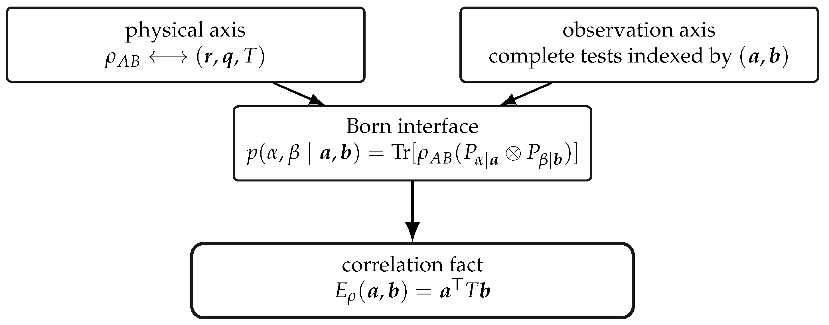
Equation (224) is the coordinate form of the dual-axis fact law. The matrix T is the physical correlation map of ; the pair specifies the two local tests on the observation axis; and the scalar is the correlation formed when those two structures meet at the Born interface. It is not a distance between settings. It is an oriented contraction of a physical correlation tensor with an observation dyad. For the singlet, , so the contraction becomes the negative Euclidean inner product . Bilinearity is not separately assumed; it follows from the Pauli expansion and the trace pairing.
21. Rotational Symmetry and the Singlet Cosine Law
Theorem 27
(Uniqueness of the singlet correlation). If a two-qubit physical state is invariant under joint rotations and perfectly anticorrelated for every equal-axis pair of binary tests, then
and hence
Proof.
A joint rotation sends , , and . Invariance under every rotation forces the two vectors to vanish. It also places T in the commutant of the irreducible three-dimensional rotation representation, so . Perfect equal-axis anticorrelation gives for every unit . Therefore , and 12 gives the stated laws. □
The associated state is
The cosine is thereby fixed in two stages. Rotational symmetry reduces the physical correlation tensor to a scalar multiple of the identity; perfect equal-axis anticorrelation fixes that scalar; the Born interface then contracts the two directions on the Bloch observation sphere.
Summing Eq. (226) over the remote outcome gives
Each marginal is independent of the remote observation state. Nonseparable correlation and relativistic no-signaling therefore coexist in the same dual-axis law.
22. CHSH Bounds and Local Noncommutativity
A Bell-local model asks for four context-independent scalar values on one probability space. Any local stochastic response can be determinized by adjoining its local random seeds to the hidden state, so it is enough to prove the bound at deterministic extremal responses. At each enlarged hidden state ,
and therefore
Exactly one bracket in the first line vanishes. Averaging any positive, setting-independent density , define
The pointwise identity therefore gives the classical inequality
Quantum binary observables retain the full projective geometry. Let , , , and , and define
For , the same signed combination is
Thus CHSH is not a single spatial separation and not a probability by itself. It is the oriented sum of four physical–observation pairings,
The signs compare four incompatible observation contexts against the same physical correlation tensor. The resulting value measures whether those four context-indexed facts can be represented by one positive global table of context-independent local answers.
Theorem 28
(Dual-axis Tsirelson theorem). Every state and every four local binary tests generated by the quantum dual-axis representation satisfy
and equality is attainable.
Proof.
Direct expansion of Eq. (235) gives
Since every binary Hermitian observable has norm one,
Consequently and . For every density operator , . By Proposition 14, the singlet is an admissible preparation. Choose the four coplanar directions
The singlet cosine law then gives
Thus the operator bound is attained. □
Figure 4.
Coplanar local observation directions attaining the Tsirelson bound. Each site uses incompatible orthogonal tests, and the directions at the second site bisect those at the first.
Figure 4.
Coplanar local observation directions attaining the Tsirelson bound. Each site uses incompatible orthogonal tests, and the directions at the second site bisect those at the first.
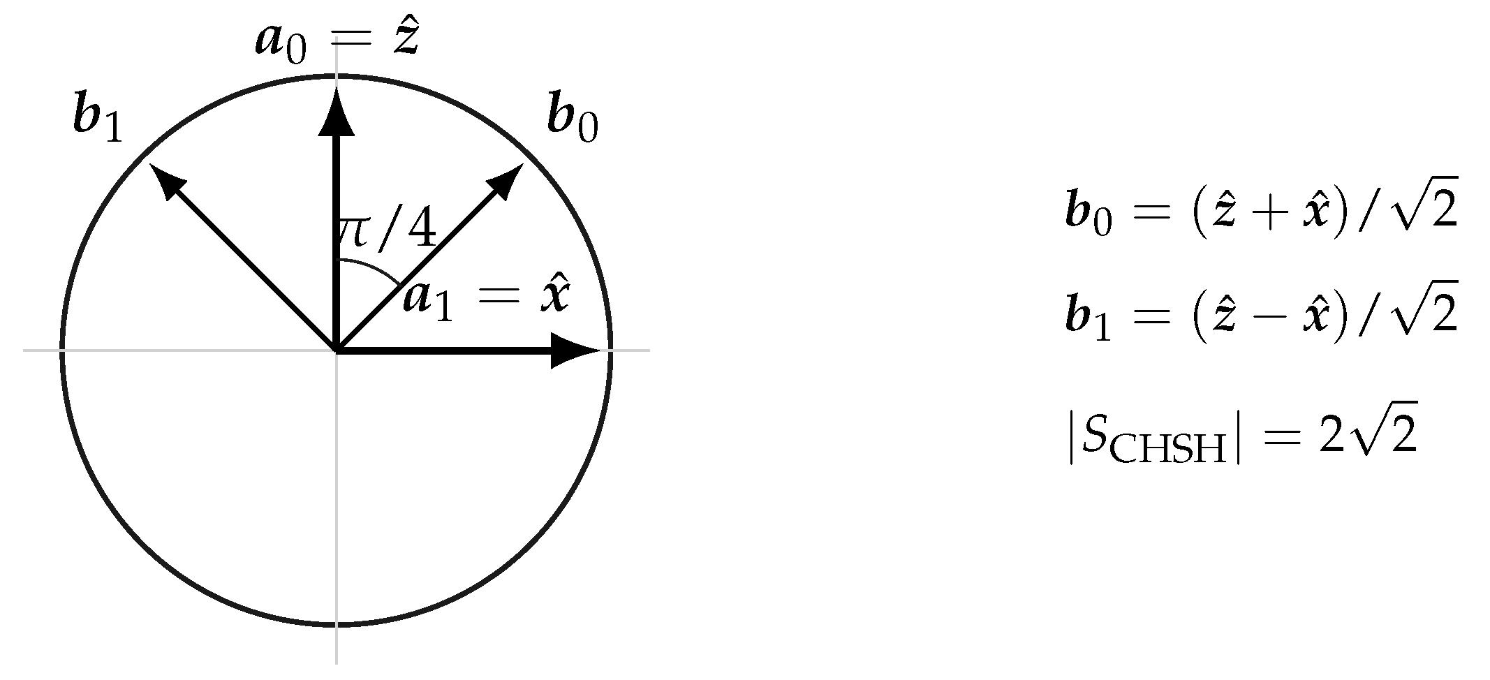
For Bloch observables,
23. The State-Dependent Spectral Boundary
Let be the eigenvalues of .
Theorem 29
(Dual-axis CHSH spectral criterion). The maximal CHSH value of a two-qubit state, optimized over all nondegenerate rank-one projective binary tests of Eq. (136), is
Hence the state violates a CHSH inequality exactly when .
Proof.
By Theorem 26,
There are orthonormal vectors and such that
For fixed , align with and with . Optimizing gives
For the singlet , all three eigenvalues equal one and the spectral criterion gives . For a general state, the two leading principal axes of the physical correlation ellipsoid determine its exact CHSH capacity.
The successive constructions can now be gathered without suppressing the steps that produced them.
Theorem 30
(Quantum representation on an enriched dual-axis interface). Let a nontrivial canonical dual-axis law satisfying the PODA Axiom admit the enrichment conditions stated in Axiom 10, Axiom 11, Axiom 13, Axiom 14, Axiom 16, Axioms 18–22. Then:
- (i)
- the scalar algebra of coherent binary response is uniquely isomorphic to ;
- (ii)
- normalized pure binary observation events form ;
- (iii)
- the probability law on every generated complex composite of dimension at least three, and by marginal descent on each binary factor, has the Born trace form;
- (iv)
- every two-qubit correlation has the universal contraction ;
- (v)
- joint rotational invariance and perfect equal-axis anticorrelation force ;
- (vi)
- every CHSH expression obeys , the bound is attainable, and the exact optimum for a state ρ is .
Proof.
Coherent response and full circular phase give item (i) by Theorem 12. Complete ray identity, the invariant Hermitian form, and compact irreducible mixing give item (ii) by Theorem 15. Independent composition produces ; refined-test completeness, contextual probability, coarse graining, and response-event consistency then yield the projector measure of Theorem 23. Gleason representation and composite marginal consistency give item (iii) by Theorem 24 and Corollary 6. The Pauli expansion and Born pairing give item (iv) in Theorem 26; rotational symmetry and equal-axis anticorrelation give item (v) in Theorem 27. Finally, the squared Bell operator proves the universal bound, Proposition 14 supplies an attainable singlet preparation, and Theorem 29 gives the exact state-dependent optimum. This proves item (vi). □
23.1. The Compact Quantum Representation and Its Dynamical Extension
Two features of the representation theorem are essential. The circle is the entire scalar-phase group, not merely a subgroup of a larger one. Composite tests also cover the full projective lattice rather than product tests alone. The first condition fixes the scalar algebra; the second provides the domain on which probability assignments acquire their trace representation.
The same Hermitian geometry also gives the PTFE of Eqs. (99) and (). Its relation to the Schrödinger branch can therefore be collected with the probability and correlation results without introducing a second geometry.
Corollary 9
(Representation with reversible physical dynamics). Under the conditions of Theorem 30, the compact quantum realization has the complex scalar field, binary projective geometry, the Born trace pairing, and the attainable Tsirelson boundary. If its reversible transformations also admit the temporal realization of 11, its physical propagation has the Schrödinger form. On a smooth reversible observation-test orbit the same propagation has the covariant form
Phase transport, physical propagation, and event probability are thus compatible laws on the same typed physical–observation architecture.
Proof.
Theorem 30 gives the scalar, projective, probabilistic, and correlation conclusions. The invariant Hermitian metric is exactly the metric used to differentiate reversible temporal composition in Theorem 25; Lemma 3 first establishes that the same transformation propagates the physical density operator. No second Hilbert geometry is introduced. Changing to the observation frame gives Eq. (188) by direct differentiation. The Born trace pairing is invariant under simultaneous changes of that frame, and hence its correlation bound is preserved. For a time-dependent state the spectral criterion applies to at each specified time and to the chosen family of complete local tests. □
The corollary combines the static representation with reversible temporal propagation. Its predictions in that sector agree with ordinary coherent quantum theory. Event-level deviations are not consequences of this compatibility result and remain separate from the present foundation.
24. The Dual-Axis Meaning of Bell Violation
Proposition 15
(Joint necessity of physical nonseparability and observational incompatibility). In a CHSH experiment:
- every separable physical state satisfies for all local tests;
- if the two tests commute at either site, every physical state satisfies .
Proof.
For a separable state of the form Eq. (218), each product term factorizes into local expectations in . The CHSH expression is multiaffine in those four numbers, so its maximum on their hypercube occurs at a vertex. The vertices are precisely the scalar assignments obeying Eq. (234); convex mixtures retain the bound. If a local pair commutes, one commutator in Eq. (239) vanishes, giving and . □
Both conditions are necessary, but neither is sufficient. A nonseparable physical state need not violate CHSH, and incompatible tests need not be chosen in directions that reveal a violation. The exact state criterion is ; the selected observation directions determine the realized value. Table 4 summarizes the roles of the state, test, and probability pairing.
For normalized binary pair distributions with consistent one-site marginals, Fine’s theorem states that a joint distribution for , a factorizable stochastic hidden-variable representation, and satisfaction of every CHSH inequality are equivalent [46]. A violation therefore says exactly that the context-indexed probability fibers do not glue into a positive, setting-independent local scalar section. Each realizable context retains a well-defined Born distribution, and overlapping marginals remain consistent; what is absent is a positive probability distribution over simultaneous assignments that reproduces all observed context marginals.
Bell’s hidden variable and the observation axis occupy different logical roles. In
is a proposed physical variable in the common past, whereas index objective local observation states. Bell violation does not identify these roles; it proves that their contextual records cannot be represented by the positive global scalar assignment required by Eq. (249).
25. Three Event Structures and Three Correlation Bounds
The algebraic CHSH maximum for four independent correlations is 4, and a no-signaling Popescu–Rohrlich box attains it [50]. A positive local scalar section lowers the ceiling to 2. Complex projective events joined by the Born pairing enlarge the attainable region to , while leaving it strictly below the algebraic boundary. These are not three estimates of one unspecified mechanism. They are the exact ceilings of three event structures: Boolean global assignments, complex-projective Born facts, and unrestricted no-signaling correlations. The numerical bound is therefore a signature of the geometry by which facts are formed.
The structural chain is summarized in Eq. (117); Corollary 9 includes its temporal continuation. The three CHSH bounds compare the event and probability structures rather than alternative estimates of the same unspecified interaction. A reproducible value above , with the required loopholes excluded, would contradict the stated complex-projective Born realization. If its marginals remained no-signaling, it would lie in the larger correlation domain illustrated in Figure 5.
A prescribed observation path already has the transport law derived above. An autonomous law for that path is a different task. A model with nonzero mixed curvature would also have to specify the physical coupling that produces it; the existence of two state coordinates or a curved projected ray bundle does not suffice.
26. Universality of the Natural Dual-Axis Structure
The universality of the second axis is a universality of form. The primitive sets , , and carry no discipline-specific internal structure, and the proof uses only typed products, equality of complete behaviors, quotients, and universal properties. Probability and Hilbert space arise when a particular science enriches the canonical state objects.
Corollary 10
(Value-object universality). Let Z be any set of complete scientific records and let . Every operationally role-faithful table has a terminal active typed exact realization. Its second state object is canonically bijective with the distinct complete maps realized by . It is non-singleton exactly when record formation is nontrivial; equivalently, in that case μ does not factor through .
Proof.
Apply Theorem 1 with ; the final equivalence is Corollary 1. □
The corollary permits Z to be a set of scalar outcomes, probability distributions, stochastic kernels, quantum channels, time series, images, logical valuations, control responses, biological phenotypes, or cognitive reports. Their internal mathematics can differ completely; the canonical behavioral reduction does not. The generality of PODA Theory lies at this structural level: wherever facts are formed from a role-faithful object input and a variable formation condition, the reduced law has the same dual-axis type.
The Chu-space reduction discussed in the Introduction is the common table geometry. The present physical application retains the two empirical anchors and a feasibility predicate, and lifts the result to antecedent physical identity when the compatibility condition holds. Universality concerns this form of representation, not a single dynamics shared by all of the possible value objects.
Enrichment requires its own descent and regularity conditions. A quotient may carry a quotient topology or -algebra, but smoothness, separation properties, and useful measure-theoretic regularity do not follow merely from forming the quotient set. Convex and compositional models likewise require operations compatible with the behavioral identifications. The quantum branch is one such specified enrichment; it is not the only domain in which the two-role reduction applies.
27. Empirical Consequences
The first empirical requirement is a fixed-input distinction in the complete record law. For distribution-valued records, different outcomes in repeated trials are not enough: the conditional probability laws themselves must differ beyond their statistical uncertainty. Once the physical and formation roles are independently fixed, such a distinction supplies the nonfactorization witness used in the categorical construction.
The enriched theory makes more specific predictions. Its Born pairing, singlet correlation, CHSH bounds, and reversible propagation reproduce the corresponding quantum sector. Their assumptions identify what is being tested: coherent response, complete composite events, reversible temporal composition, or a prescribed observation reference. The general quotient construction does not replace those physical conditions.
Appendix B presents a table-top experiment in which an adiabatically moving, isolated observation frame induces a geometric phase on a quantum system whose Hamiltonian vanishes. Standard quantum mechanics predicts a null phase for this configuration. The phase transport fundamental equation predicts a phase equal to half the solid angle enclosed by the frame’s Bloch-sphere trajectory. The comparison tests the operational content of observation-axis transport and establishes the observation axis as a physical entity. It does not require an event-selection law.
28. Conclusions
The starting point was a change of complete record at one independently certified physical input. Complete behavioral equivalence removes the redundant preparation and formation labels, unique descent retains their record law, and terminality makes the reduced realization canonical. Exponential transposition then identifies the surviving formation classes with distinct complete response maps. This is the observation-state object. The compatible physical anchor preserves the first axis even when the present observation family resolves only a coarser behavioral image.
The resulting physical statement is a joint record law: in an activated domain, the state observed does not by itself determine the complete fact law across changing observation conditions. Both arguments remain objective within the declared physical interpretation. Fixing an observation state recovers a unary section; allowing it to vary restores the full interface. Conditional identifiability, label-free recovery, and same-source comparison then become separate, precisely stated questions on that domain.
The quantum branch gives this structure a specific representation. Full circular phase within the associative division-response class selects . Reversible mixing and ray identity supply projective binary geometry; bilinear universal composition, complete tests, and event consistency supply the setting for the Born trace representation. The correlation tensor gives the singlet cosine law, the Tsirelson ceiling, and the exact state-dependent CHSH optimum. Nonseparability and local test incompatibility are necessary resources for a violation, whereas a positive global answer distribution is the structure excluded by the complete CHSH test.
The temporal continuation uses that same Hermitian geometry. Reversible covariance first relates response transformations to physical preparation changes. Differentiable temporal composition then gives a Hermitian generator and the Schrödinger equation. In a moving observation frame, separates physical propagation from frame transport. The nonrelativistic spatial assumptions fix the kinetic term once the mass is specified, and the rotating binary example shows how two changing states can produce a constant probability record. None of these steps identifies phase transport with an autonomous event-selection law.
The familiar quantum examples can be located within this division of roles. In a two-path experiment, coherent preparation supplies the amplitudes and the complete test determines whether the recorded distribution retains their interference term. A which-path instrument changes the experimental interaction or the retained record; this is not a claim that a passive choice of description changes an otherwise identical experiment. In the cat experiment, unitary evolution, a macroscopic outcome distribution, and an outcome-conditioned update are different parts of the description. Their typing clarifies the question of a definite record but does not itself select one outcome. In a Bell experiment, one nonseparable preparation and two local tests produce correlations with no-signaling marginals, without a positive global assignment of all incompatible local answers.
Relativistic and internal gauge geometries enter through the bundle-pullback construction. Their symmetry groups and connections retain their physical meaning, while fixed-observation sections recover their supplied sector geometry. This establishes a common representation of states and transport, not the Einstein or Yang–Mills equations or the matter content and couplings of the Standard Model. A further dynamical theory would have to select an action, for example within the schematic class
Here denotes candidate matter or response fields, g a metric, the remaining coupling and background data, and the chosen integration measure. No particular Lagrangian is fixed in the present paper. Recovery of the observed gravitational and gauge sectors, compatible limiting procedures, and an independently calculated mixed-curvature response are requirements on such a continuation.
The geometric-phase experiment makes the physical reality of the observation axis concrete. A system held at zero Hamiltonian accumulates a phase that depends only on the geometry of the frame’s closed path, in sharp contrast to the null prediction of standard quantum mechanics. The phase is a holonomy of the observation-axis connection. A positive result establishes the observation axis as an irreducible physical entity and confirms the PTFE as a law of quantum kinematics. Departures from the predicted solid-angle law would constrain the implementation model rather than an autonomous event law.
The foundation is thus a canonical state architecture together with a specified coherent realization. It retains the physical source, gives the conditions of observation a behavioral state identity, and distinguishes the laws that evolve a state, compare its representations, and form its probabilities. An event-selection dynamics can be developed on this foundation, but is not a premise of the state construction or the geometric-phase experiment.
Appendix A. Proofs of the Categorical Construction
The categorical constructions below generate the canonical typed behavioral realization from an operationally role-faithful complete record. Together with the compatible antecedent physical interface of Proposition 9, they generate a canonical model of the PODA Axiom.
Appendix A.1. Kernel Pairs and Coequalizers
For a map , its kernel pair in is with the two coordinate projections to U. The quotient of U by this equivalence relation is the coequalizer of those projections. The aggregate maps and were defined in Equation (12). The relations in Equations (10) and (11) are exactly and . Hence and are their coequalizers. The induced maps and are injective; this is the regular-epimorphism–monomorphism factorization of the two transposes in .
Appendix A.2. Proof of the Terminal Universal Property
The objects and morphisms of are given in 3. Let be any object. If , then for every ,
Thus , so is constant on every -fiber. Since is surjective, there is a unique map with . Because is surjective, so is u. The same argument gives a unique surjection with .
For any , choose with and . Then
Hence , and is a morphism to the canonical realization. The anchor equations and surjectivity of and force u and v uniquely, proving terminality.
It remains to identify their fibers. If , choose with and . Then , so the primitive rows agree. For any , choose a with ; exactness gives
Conversely, equality of the two G-rows implies equality after evaluation at every , hence and . This proves Equation (30); the proof of Equation (31) is symmetric. Since u and v are already surjective, the realization is biextensional exactly when both maps are bijective. Their inverses then define the unique isomorphism to the canonical realization.
Appendix A.3. Proof of Formation-Side Minimality
Suppose . Choose with and . For every , set . Then
Thus and , proving injectivity. Surjectivity of holds by the definition of , proving Theorem 1(iii).
The proof that the row transpose in Equation (33) is injective is symmetric. If , choose with and . Equality on every gives for every , so and .
For a complete implementation , define if . The formula
is well defined and injective, and surjectivity of makes it bijective. Hence every complete implementation becomes uniquely isomorphic to the canonical behavior space after quotienting its duplicate labels. This proves the observation-state identity used in the main text.
Appendix A.4. Proof of the Activation Equivalences
If Equation (4) holds, then , so and . Conversely, two distinct classes in have different complete columns; hence some witnesses unequal entries. The bijection gives the equivalence with .
If , every slice equals h, so and are singletons. Conversely, if , define ; then . Composing with proves the corresponding primitive factorization. Conversely, a primitive factorization makes every row constant on , so all columns are equivalent and is a singleton. This proves the first cycle of equivalences in Corollary 1.
A strong primitive witness descends to two points with unequal values under F. Conversely, suppose such reduced points exist. Choose with and with . Then
so the lifted entries form a strong witness. Finally, the surjection admits a factorization exactly when F is constant on each of its fibers. This is equivalent to the absence of a reduced strong witness and completes the proof.
Appendix A.5. Proof of Empirical-Cover Invariance
Indeed, equality of the two primed rows is, by injectivity of , equality of the unprimed rows after evaluation at every ; surjectivity of v makes this equivalent to equality at every . Hence is well defined and injective; surjectivity of u makes it surjective, and surjectivity of makes the anchor equation determine it uniquely. The symmetric argument, using surjectivity of u, proves the corresponding claims for .
For quotient classes,
which proves Equation (59). Because maps bijectively onto and ⊥ to , the product bijection maps onto and its restriction is . Restricting the descended-law identity gives Equation (61). Witnesses lift through the surjections and descend through Equation (56); injectivity of preserves inequality, while and preserve the strong–weak distinction.
Appendix A.6. External Physical Identity
Condition (62) says , so quotient factorization gives a unique with ; it is surjective. Define
Compatibility on the first side and complete column equivalence on the second make this independent of representatives. Evaluating on the surjective image of proves both equalities in Equation (63). Taking inverse images of gives Proposition 9; the pullback proof is identical to the canonical case. If two formation states give the same maps on , surjectivity of r gives equality of their primitive columns and hence equality in ; the formation-side transpose is injective. Finally, is injective exactly when equality of row behaviors also implies equality under r, proving Proposition 9.
Appendix B. Observation-Frame-Induced Geometric Phase: a Table-Top Test of the PTFE
The PTFE of Eq. (102) predicts that the motion of an observation frame induces a geometric phase on a quantum system, even when the system Hamiltonian vanishes identically. This appendix turns that prediction into a table-top experiment executable on existing superconducting quantum processors. The distinction from standard quantum mechanics is sharp: a passive change of observation frame is a coordinate transformation that leaves every physical prediction invariant, whereas the PTFE treats the frame as a physical entity whose motion leaves a measurable geometric imprint.
Appendix B.1. Physical Setup and the Role of the Observation Axis
Two independently controllable quantum systems are required. A system qubit S is realized by a superconducting transmon with transition frequency , representing the physical axis. A frame qubitF is realized by a second transmon or tunable resonator, representing the observation frame. The two are engineered to have negligible direct coupling: their interaction is mediated exclusively by the observation interface, implemented as a calibrated dispersive coupling that is switched off during the phase-accumulation window, or as a measurement-and-feedback loop that establishes the same interface. The system Hamiltonian is held at throughout the protocol.
The experiment is a direct test of the algebraic structure of the dual-axis connection. In the language of Section 18.2, the frame’s Bloch vector traces a closed path on . The PTFE comparison factor associated with this path is the holonomy
where and are the polar and azimuthal angles of the frame’s Bloch vector. For a path that winds once at fixed around the polar axis,
where is the solid angle enclosed by the path on the Bloch sphere. Standard quantum mechanics predicts a null phase for the system qubit throughout the protocol.
Appendix B.2. Protocol
The protocol has five steps.
- (i)
- Initialization. Prepare the system qubit in . Prepare the frame qubit in the reference state , corresponding to the north pole of its Bloch sphere.
- (ii)
- Frame trajectory. Adiabatically drive the frame qubit along a closed path on its Bloch sphere. For example, at fixed polar angle , rotate the frame’s Bloch vector around the z-axis by . The drive must be slow compared to the frame qubit’s energy gap to ensure adiabaticity, but fast compared to the system qubit’s coherence time.
- (iii)
- System evolution. During the frame trajectory, hold the system Hamiltonian at . The system undergoes no dynamical evolution. Its state evolves solely according to the PTFE.
- (iv)
- Ramsey interferometry. After the frame returns to its initial state, perform Ramsey interferometry on the system qubit: apply a pulse, wait for a fixed delay, apply a second pulse, and measure the population of . The phase of the resulting interference fringe is the accumulated geometric phase .
- (v)
- Variation. Repeat the protocol for several values of . Plot the measured phase shift as a function of .
Appendix B.3. Predictions
Standard quantum mechanics treats the observation frame as a passive coordinate choice. A change of frame induces a unitary transformation on the state vector, but every physical prediction—including the phase of an interference fringe—remains invariant. In particular, if the system Hamiltonian vanishes and the system and frame are uncoupled, the system’s state does not change, and the measured Ramsey phase is identically zero.
Prediction 1
(Standard quantum mechanics). The measured geometric phase is identically zero for every frame trajectory.
The PTFE instead predicts a nonzero, geometry-dependent phase. The phase shift in the Ramsey fringe is
Prediction 2
(PTFE). The measured phase shift depends only on the solid angle Ω enclosed by the frame’s Bloch-sphere trajectory, according to Eq. (A4). It is independent of the duration of the frame’s motion, the system’s energy, and the specific shape of the closed path.
The two predictions are mutually exclusive. A measurement of a nonzero phase shift that follows Eq. (A4) confirms the PTFE and establishes the observation axis as a physical entity. A null result falsifies the PTFE.
Appendix B.4. Control and Calibration
Several controls are essential to exclude alternative explanations.
- (i)
- Null test. With the frame qubit held stationary ( or no drive), the measured phase must be zero.
- (ii)
- Direct-coupling test. Verify independently that the system and frame qubits have no residual direct coupling by measuring the system’s phase with the frame driven but the observation interface disconnected.
- (iii)
- Frame calibration. Calibrate the frame qubit’s Bloch-sphere trajectory using quantum state tomography, ensuring that the intended solid angle is accurately realized.
- (iv)
- Ramsey calibration. Calibrate the Ramsey interferometer using a known dynamical phase (for example, a calibrated Z-rotation on the system qubit) to establish the phase-to-fringe conversion factor.
- (v)
- Randomized paths. Use randomly generated closed paths with the same enclosed solid angle but different shapes. The PTFE predicts the same holonomy for all such paths, providing a strong consistency check.
- (vi)
- Frequency scan. Verify that the measured phase does not depend on the duration of the frame drive when the frame path is fixed.
Appendix B.5. Technical Feasibility
The experiment is executable on existing superconducting quantum processors with the following specifications: qubit coherence time ; single-qubit gate fidelity ; readout fidelity ; adiabatic frame drive with duration ; phase measurement precision . These requirements are met by state-of-the-art transmon processors.
Appendix B.6. Experimental Feasibility and Systematic Errors
A critical reader may question the feasibility of achieving for a superconducting transmon. While a bare transmon possesses an intrinsic finite transition frequency, we envisage implementing this protocol by applying a continuously calibrated dynamical decoupling sequence (e.g., a spin-echo or XY-8 sequence) synchronized with the frame drive. This effectively zeros the time-averaged dynamical phase while preserving the geometric holonomy. Furthermore, the residual cross-Kerr coupling between the system and the frame is independently calibrated before the closed-path drive, and its dynamical contribution is subtracted from the measured phase.
To mitigate non-adiabatic transitions during the frame’s trajectory, we adopt a Shortcuts-to-Adiabaticity (STA) protocol. By adding a counter-diabatic driving field to the frame qubit, the system can follow the instantaneous eigenstates of the frame within a significantly reduced evolution time, ensuring that the geometric phase is accumulated faster than the system’s decoherence rate. Finally, a differential measurement scheme is employed to isolate the geometric contribution. Two closed paths with identical enclosed solid angles but opposite orientations are driven sequentially. The dynamical phases accumulated in both paths cancel out, while the geometric holonomy changes sign. The measured phase difference therefore provides a direct, background-free readout of the PTFE holonomy, independent of pulse calibration errors or slow frequency drifts.
Appendix B.7. Falsifiability and the Physical Reality of the Observation Axis
The experiment is a direct, table-top test of the PTFE. It does not rely on any dynamical evolution of the system, any specific form of the system–frame interaction, or any cosmological observation. The two predictions are mutually exclusive, and the phase predicted by the PTFE is fixed by the geometry of the frame’s closed path alone. The experiment therefore provides a decisive, falsifiable test of the physical reality of the observation axis and of the PTFE as a law of quantum kinematics.
A positive result would establish a geometric phase that is not associated with any dynamical evolution of the system, but solely with the motion of the observation frame. This directly contradicts the standard quantum mechanical treatment of observation frames as passive coordinate choices. A null result would falsify the PTFE in its stated scalar or projective form.
Parameter-Free Prediction and the Numerical Constant
To demonstrate the falsifiability of the framework, we derive the exact numerical constant expected in a table-top implementation. The observation-axis connection on the Bloch sphere is . For a frame trajectory that adiabatically winds once around the polar axis at a fixed polar angle , the accumulated geometric holonomy is
To isolate a non-trivial geometric constant that is unambiguously distinguishable from zero, we choose a specific polar angle such that . This yields the parameter-free prediction
Standard quantum mechanics, treating the observation frame as a passive coordinate choice, predicts a null phase shift () for this configuration. Observing a phase shift of (within the calibrated error bars of the differential measurement scheme) would confirm the PTFE, whereas a null result would sharply falsify the dual-axis mechanism.
References
- Shannon, C. E. A mathematical theory of communication. Bell Syst. Tech. J. 1948, 27, 379 and 623. [Google Scholar] [CrossRef]
- Fisher, R. A. On the mathematical foundations of theoretical statistics. Philos. Trans. R. Soc. Lond. A 1922, 222, 309. [Google Scholar] [CrossRef]
- Wald, A. Statistical Decision Functions; Wiley, New York, 1950. [Google Scholar]
- Kiefer, J.; Wolfowitz, J. Optimum designs in regression problems. Ann. Math. Stat. 1959, 30, 271. [Google Scholar] [CrossRef]
- Chernoff, H. Sequential design of experiments. Ann. Math. Stat. 1959, 30, 755. [Google Scholar] [CrossRef]
- Shannon, C. E. Channels with side information at the transmitter. IBM J. Res. Dev. 1958, 2, 289. [Google Scholar] [CrossRef]
- Gelfand, S. I.; Pinsker, M. S. Coding for channel with random parameters. Probl. Control Inf. Theory 1980, 9, 19. [Google Scholar]
- Le Cam, L. Sufficiency and approximate sufficiency. Ann. Math. Stat. 1964, 35, 1419. [Google Scholar]
- Bohr, N. The quantum postulate and the recent development of atomic theory. Nature 1928, 121, 580. [Google Scholar] [CrossRef]
- Einstein, A.; Podolsky, B.; Rosen, N. Can quantum-mechanical description of physical reality be considered complete? Phys. Rev. 1935, 47, 777. [Google Scholar] [CrossRef]
- E. Schrödinger, Discussion of probability relations between separated systems. Math. Proc. Camb. Philos. Soc. 1935, 31, 555. [CrossRef]
- Bell, J. S. On the Einstein Podolsky Rosen paradox. Physics 1964, 1, 195. [Google Scholar] [CrossRef]
- Clauser, J. F.; Horne, M. A.; Shimony, A.; Holt, R. A. Proposed experiment to test local hidden-variable theories. Phys. Rev. Lett. 1969, 23, 880. [Google Scholar] [CrossRef]
- Kochen, S.; Specker, E. P. The problem of hidden variables in quantum mechanics. J. Math. Mech. 1967, 17, 59. [Google Scholar] [CrossRef]
- Blackwell, D. Equivalent comparisons of experiments. Ann. Math. Stat. 1953, 24, 265. [Google Scholar] [CrossRef]
- Krantz, D. H.; Luce, R. D.; Suppes, P.; Tversky, A. Foundations of Measurement, Vol. I; Academic Press: New York, 1971. [Google Scholar]
- E. Torgersen, Comparison of Statistical Experiments; Cambridge University Press: Cambridge, 1991.
- Barrett, J. Information processing in generalized probabilistic theories. Phys. Rev. A 2007, 75, 032304. [Google Scholar] [CrossRef]
- Chiribella, G.; D’Ariano, G. M.; Perinotti, P. Informational derivation of quantum theory. Phys. Rev. A 2011, 84, 012311. [Google Scholar] [CrossRef]
- Masanes, L.; Müller, M. P. A derivation of quantum theory from physical requirements. New J. Phys. 2011, 13, 063001. [Google Scholar] [CrossRef]
- Spekkens, R. W. Contextuality for preparations, transformations, and unsharp measurements. Phys. Rev. A 2005, 71, 052108. [Google Scholar] [CrossRef]
- Abramsky, S.; Brandenburger, A. The sheaf-theoretic structure of non-locality and contextuality. New J. Phys. 2011, 13, 113036. [Google Scholar] [CrossRef]
- Abramsky, S.; Coecke, B. Categorical quantum mechanics. In Handbook of Quantum Logic and Quantum Structures: Quantum Logic; Engesser, K., Gabbay, D. M., Lehmann, D., Eds.; Elsevier: Amsterdam, 2009; pp. 261–324. [Google Scholar] [CrossRef]
- Selby, J. H.; Schmid, D.; Wolfe, E.; Sainz, A. B.; Kunjwal, R.; Spekkens, R. W. Accessible fragments of generalized probabilistic theories, cone equivalence, and applications to witnessing nonclassicality. Phys. Rev. A 2023, 107, 062203. [Google Scholar] [CrossRef]
- Eilenberg, S.; Mac Lane, S. General theory of natural equivalences. Trans. Am. Math. Soc. 1945, 58, 231. [Google Scholar] [CrossRef]
- Mac Lane, S. Categories for the Working Mathematician, 2nd ed.; Springer: New York, 1998. [Google Scholar]
- Leinster, T. Basic Category Theory; Cambridge University Press: Cambridge, 2014. [Google Scholar]
- Riehl, E. Category Theory in Context; Dover: Mineola, NY, 2016. [Google Scholar]
- E. F. Moore, Gedanken-experiments on sequential machines, in Automata Studies, edited by C. E. Shannon and J. McCarthy 1956, 129–153.
- Myhill, J. 1957. Finite Automata and the Representation of Events. WADC Technical Report No. 57-624. Wright Air Development Center. [Google Scholar]
- Nerode, A. Linear automaton transformations. Proc. Am. Math. Soc. 1958, 9, 541. [Google Scholar] [CrossRef]
- Kalman, R. E. Mathematical description of linear dynamical systems. J. Soc. Ind. Appl. Math. Ser. A Control 1963, 1, 152. [Google Scholar] [CrossRef]
- Ho, B. L.; Kalman, R. E. Effective construction of linear state-variable models from input/output functions. Regelungstechnik 1966, 14, 545. [Google Scholar] [CrossRef]
- Bellman, R.; Åström, K. J. On structural identifiability. Math. Biosci. 1970, 7, 329. [Google Scholar] [CrossRef]
- Rothenberg, T. J. Identification in parametric models. Econometrica 1971, 39, 577. [Google Scholar] [CrossRef]
- Hermann, R.; Krener, A. J. Nonlinear controllability and observability. IEEE Trans. Autom. Control 1977, 22, 728. [Google Scholar] [CrossRef]
- Walter, E.; Pronzato, L. Identification of Parametric Models from Experimental Data; Springer: London, 1997. [Google Scholar]
- L. Ljung, System Identification: Theory for the User, 2nd ed.; Prentice Hall PTR: Upper Saddle River, NJ, 1999.
- Frobenius, F. G. Über lineare Substitutionen und bilineare Formen. J. Reine Angew. Math. 1878, 84, 1. [Google Scholar] [CrossRef]
- Hopf, H. Über die Abbildungen der dreidimensionalen Sphäre auf die Kugelfläche. Math. Ann. 1931, 104, 637. [Google Scholar]
- Meng, X. Mathematical and theoretical foundations of the basic phase-transport equation: A unified differential, covariant, and path-functional theory. Preprints 2026. [Google Scholar] [CrossRef]
- Gleason, A. M. Measures on the closed subspaces of a Hilbert space. J. Math. Mech. 1957, 6, 885. [Google Scholar] [CrossRef]
- Fiorentino, V.; Weigert, S. Gleason’s theorem for a qubit as part of a composite system. Phys. Rev. A 2026, 113, 062221. [Google Scholar] [CrossRef]
- Busch, P. Quantum states and generalized observables: A simple proof of the Gleason theorem. Phys. Rev. Lett. 2003, 91, 120403. [Google Scholar] [CrossRef] [PubMed]
- Davies, E. B.; Lewis, J. T. An operational approach to quantum probability. Commun. Math. Phys. 1970, 17, 239. [Google Scholar] [CrossRef]
- A. Fine, Hidden variables, joint probability, and the Bell inequalities. Phys. Rev. Lett. 1982, 48, 291. [CrossRef]
- Werner, R. F. Quantum states with Einstein-Podolsky-Rosen correlations admitting a hidden-variable model. Phys. Rev. A 1989, 40, 4277. [Google Scholar] [CrossRef] [PubMed]
- Cirelson, B. S. Quantum generalizations of the Bell inequality. Lett. Math. Phys. 1980, 4, 93. [Google Scholar] [CrossRef]
- Horodecki, R.; Horodecki, P.; Horodecki, M. Violating Bell inequality by mixed spin-1/2 states: Necessary and sufficient condition. Phys. Lett. A 1995, 200, 340. [Google Scholar] [CrossRef]
- Popescu, S.; Rohrlich, D. Quantum nonlocality as an axiom. Found. Phys. 1994, 24, 379. [Google Scholar] [CrossRef]
- M. Barr, The Chu construction. Theory Appl. Categ. 1996, 2, 17.
- Barr, M. The separated extensional Chu category. Theory Appl. Categ. 1998, 4, 137. [Google Scholar] [CrossRef]
- R. M. Wald, General Relativity; University of Chicago Press: Chicago, 1984.
- Yang, C. N.; Mills, R. L. Conservation of isotopic spin and isotopic gauge invariance. Phys. Rev. 1954, 96, 191. [Google Scholar] [CrossRef]
- Wu, T. T.; Yang, C. N. Concept of nonintegrable phase factors and global formulation of gauge fields. Phys. Rev. D. 1975, 12, 3845. [Google Scholar] [CrossRef]
- Kobayashi, S.; Nomizu, K. Foundations of Differential Geometry, Vol. I; Wiley–Interscience: New York, 1963. [Google Scholar]
- Stone, M. H. On one-parameter unitary groups in Hilbert space. Ann. Math. 1932, 33, 643–648. [Google Scholar] [CrossRef]
- B. Simon, Holonomy, the quantum adiabatic theorem, and Berry’s phase. Phys. Rev. Lett. 1983, 51, 2167–2170. [CrossRef]
- J.-M. Lévy-Leblond, Galilei group and nonrelativistic quantum mechanics. J. Math. Phys. 1963, 4, 776–788. [CrossRef]
- Hoeffding, W. Probability inequalities for sums of bounded random variables. J. Am. Stat. Assoc. 1963, 58, 13–30. [Google Scholar] [CrossRef]
Figure 5.
Three structural CHSH bounds. The numerical ceiling records the event geometry and probability-composition law: a local scalar section, complex projective Born probabilities, or the unrestricted no-signaling domain.
Figure 5.
Three structural CHSH bounds. The numerical ceiling records the event geometry and probability-composition law: a local scalar section, complex projective Born probabilities, or the unrestricted no-signaling domain.
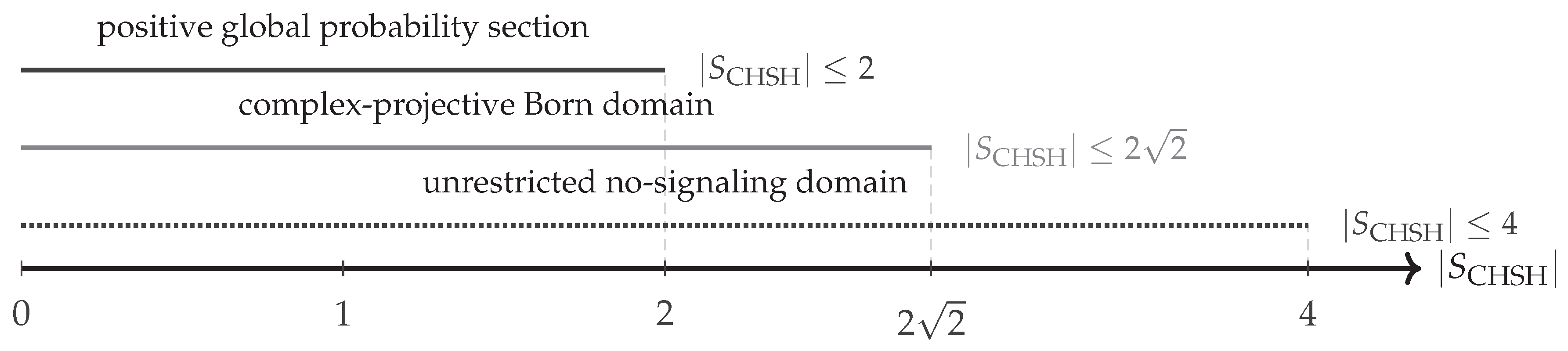
Table 4.
Distinct roles in a Bell experiment. The observation state is the complete local test; an event projector is one component selected by an outcome.
Table 4.
Distinct roles in a Bell experiment. The observation state is the complete local test; an event projector is one component selected by an outcome.
| Structural layer | Mathematical object | Role in the correlation |
|---|---|---|
| Physical axis | and T | Carries the separable or nonseparable joint state and its correlation ellipsoid |
| Observation axis | Tests indexed by | Carries local alternatives and their compatibility relations |
| Dual-axis interface | Forms context-indexed probabilities with consistent marginals | |
| Fact layer | and | Produces experimentally comparable correlations and bounds |
Disclaimer/Publisher’s Note: The statements, opinions and data contained in all publications are solely those of the individual author(s) and contributor(s) and not of MDPI and/or the editor(s). MDPI and/or the editor(s) disclaim responsibility for any injury to people or property resulting from any ideas, methods, instructions or products referred to in the content. |
© 2026 by the authors. Licensee MDPI, Basel, Switzerland. This article is an open access article distributed under the terms and conditions of the Creative Commons Attribution (CC BY) license (http://creativecommons.org/licenses/by/4.0/).
Copyright: This open access article is published under a Creative Commons CC BY 4.0 license, which permit the free download, distribution, and reuse, provided that the author and preprint are cited in any reuse.