

Submitted:
04 September 2026
Posted:
07 September 2026
You are already at the latest version
Abstract
Local sequence carries information about the backbone dihedrals out to a window radius of about 8 residues.¹ How much of that information becomes accuracy, and what the remainder consists of, are separate questions. Working at a fixed radius of 8 on 2,588 enzyme chains, I ask both. A model with 27,000 weights reaches a mean absolute error of 22.7° for φ and 46.8° for ψ on held-out enzyme cores, against 28.2° and 66.3° for the best constant predictor. Eleven interventions were then tried against that model; ten changed nothing. Capacity does not help — a convolutional control with 116,068 weights and none of the model's constraints scores 23.5° and 47.4°. Reach does not help: running the same weight tensors repeatedly extends the receptive field to 64 residues with no parameters added at all, and buys 0.6° on ψ and 0.1° on φ over three seeds. The one large effect is conditioning on secondary structure, worth 5.9° on ψ — but only when the true class is supplied. A second, independent route to the same information confirms it: supplying each strand residue's true β-pairing partner, extracted from deposition records, is worth 7.65° on ψ and 13.29° on ψ sheet, and a control reduces the channel to a single bit — that a partner exists — recovering the whole effect with 72 weights while the partner's identity contributes nothing. A class predictor in the same architecture reaches Q3 58.0% while assigning sheet to none of 82,949 test residues; class-balancing lifts sheet recall to 51.0% at the cost of 56.3% overall error, and both make the torsion prediction worse than no class channel at all.To calibrate what any of this means I measure a reproducibility floor on a separately assembled redundant set: 1,092 pairs of independently deposited structures sharing ≥90% sequence identity, of which 1,069 could be measured from coordinates rather than from binned angles, giving 131,771 scored core positions. Half of all core residues agree to within 3.6° in φ and 3.3° in ψ; the means are 6.0° and 5.8° and the 90th percentiles 12.4° and 11.9°. The model therefore sits at 3.8 and 8.0 times the floor in the mean, and at 4.4 and 13.5 times at the 90th percentile, capturing a quarter of φ's and a third of ψ's available range. Crystal packing is the largest environmental term and it is small: pairs differing in space group disagree by about two degrees more than pairs sharing one, against a model error of 22.7°. The residual is therefore missing information rather than conformational indeterminacy or environment — which, with the locality results, places that information in the chain but outside any local window. Two signatures point at a single ceiling: two mechanically unrelated interventions, one at the readout and one extending reach, each remove three to four degrees of β-sheet error and combining them removes less than reach does alone; and replacing the architecture outright decorrelates the model's errors less than changing its random seed does.
Keywords:
protein conformation
; protein structure
; secondary
; amino acid sequence
; models
; molecular
; computational biology
; neural networks
Introduction
A companion study measured how far along the chain a backbone dihedral is written, and found that φ and ψ both saturate at a window radius of about 8 residues, beyond which additional sequence context costs accuracy rather than leaving it unchanged [1]. That result is about reach, expressed in bits: it says where the local signal ends. It says nothing about how much of the signal inside that window a model can convert into angular accuracy, nor what the part it cannot reach is made of.
Those are the questions here, and they need a different currency. Information in bits is the right measure for locating a signal’s endpoint, because it is insensitive to how concentrated the target already is. Mean angular error is the right measure for asking how close a prediction gets, and it is the quantity that matters to anything built downstream from predicted angles. The two are not interchangeable, and a result in one does not transfer to the other.
The second question is the harder one, and the literature offers less help with it. Predictors of backbone angles report mean absolute errors of roughly 15–20° for φ using deep architectures over evolutionary profiles and predicted contact maps [2], with single-sequence variants where no alignment is available [3]. None reports what error would be achieved by a perfect predictor. Without that reference an error figure cannot be read: 20° is either close to optimal or far from it depending on how much φ varies between structures of the same sequence, and that quantity is not established.
It can be measured. The same sequence crystallised more than once gives structures that differ, and the size of that difference is a floor no sequence-only predictor can go below. Conformational variation between independent determinations of the same protein is well documented—it underlies the coil-library approach to intrinsic propensities [4,5], and fold-switching proteins adopt genuinely distinct native structures under different conditions [6]—but I am not aware of a published estimate of it expressed as a per-residue dihedral disagreement, on the same population and in the same units as prediction error is reported.
This paper does four things. It exhausts a set of architectural and input-side interventions against a model held at the saturation radius, reporting one modest success and ten failures, because the failures locate the constraint more sharply than the success does. It measures the reproducibility floor over a thousand pairs of independently deposited structures and uses it to calibrate every error figure, with the crystallographic conditions attached so that the environmental component can be quantified rather than assumed. It isolates why one intervention that clearly works—conditioning on secondary structure—cannot be made to work from sequence alone, which turns out to follow from the geometry rather than from any deficiency of the predictor. And it shows why the natural remedy for that class of failure is unavailable: the residues a local model gets wrong are not a property of the model.
Throughout, the model is a per-residue-type architecture described in Methods. It is used because it is small enough that capacity claims are testable rather than assumed, and because its constraints are individually removable, so each can be tested as a hypothesis. It is not offered as an advance in predictive accuracy; on this dataset it is level with an unconstrained convolutional control, and Limitations reports where it is worse.
Materials and Methods
Data
All structures are public depositions in the Protein Data Bank [7]. Chains were restricted to enzymes, identified by an EC number recorded in a COMPND record. The restriction reflects the intended application; its consequences for generality are addressed in Limitations. Of the candidate chains, 4,858 were rejected as non-enzymes, 93 as unreadable, 22 as too short and 11 as too long, leaving 2,588 chains and 797,541 residues: 2,050 training, 266 validation and 272 test chains, and 630,643, 83,949 and 82,949 residues. Splits are assigned deterministically by a hash of the chain identifier. The composition is 33% helix, 12% sheet and 55% coil.
Backbone dihedrals were computed from deposited coordinates and secondary structure taken from the HELIX and SHEET records, reduced to three classes. The assignment is therefore the depositors’ rather than one recomputed by a single algorithm [8].
Angles were discretised into 72 bins of 5°. A bin’s representative angle is its centre, reported in (−180°, 180°]. φ is undefined at the N-terminal residue and ψ at the C-terminal residue; those positions are excluded throughout and are not counted in any reported n.
All accuracy figures are quoted over helix and sheet residues only—36,475 φ and 36,406 ψ values in the test split. Coil is excluded from scoring and from the loss, a choice tested in Results. Every number in this paper is a mean absolute circular error in degrees over that population unless stated otherwise, and every floor figure is measured over the same population so that the two are comparable.
The Model
Each residue holds a state vector of 36 values, and each layer replaces that state by a weighted combination of the states of its neighbours within a radius of 8—17 offsets including itself. Two properties define the architecture.
First, the weight applied to a neighbour’s contribution is selected by that neighbour’s residue type, so the parameters form an array W[type][layer][offset][slot]: each of 22 residue types carries its own set, and a type’s parameters travel with it wherever in a chain it occurs. Second, combination is element-wise—slot b of a neighbour reaches only slot b of the receiving residue—so the 36 slots are 36 independent scalar networks and no weight anywhere lets one slot influence another.
The configuration used throughout is two weight layers (one hidden), radius 8, tanh activation on the hidden layer, and an input state of all ones, giving 22 × 2 × 17 × 36 weights plus biases = 27,000 parameters. The final layer’s 36 values are the logits directly; there is no activation on them.
The 36 slots encode the angle as a thermometer code in which Hamming distance equals circular bin distance, and decoding is by nearest codeword under the full quadratic criterion, argmax over b of 2·p·c<sub>b</sub> − ‖c<sub>b</sub>‖2, where p is the vector of predicted bit probabilities. Dropping the norm term biases decoding toward high-weight codewords and is a mistake worth naming, since the term vanishes only for codes of constant weight, which this is not.
The forward pass runs over every residue including coil, so a core residue’s window sees its coil neighbours; only the loss is restricted. Training uses Adam [10], mini-batches of 16 chains, early stopping on validation negative log likelihood with patience 8 and a cap of 40 epochs. Unless stated, figures are means over seeds 11, 23 and 37 with the range given.
Interventions
Mixing head. One shared 36 × 36 layer applied to the final logits, at the point where 36 independently estimated slots must become one codeword. It is shared across residue types rather than per-type—the latter would be 484,704 weights, eighteen times the trunk—and it is initialised to the identity, so the arm is a strict superset of the model it is compared with and epoch 0 reproduces it exactly. A nonlinear variant adds a residual 64-unit tanh layer with zeroed output weights, also starting at the identity. Costs are 1,332 and 4,708 weights.
Recurrence. The same 22 weight tensors are applied repeatedly, with the logistic transform of the raw logits from one pass becoming the input state of the next; the first pass starts from all ones, as the base model does. Weights are shared across passes, so the parameter count remains 27,000 at any number of passes while the receptive radius grows by layers × radius = 16 residues per pass. Gradients propagate through every pass: the quantity needed is the gradient with respect to a layer’s input state, which the base backward pass already computes and discards. This is not a depth increase—depth would give each layer independent parameters—and it is not a two-stage cascade, because no intermediate is required to be a good prediction of anything.
Secondary-structure conditioning. Two forms. Per-class models train separate models restricted to helix and to sheet targets. Class as input replaces the all-ones input state with a codeword encoding the residue’s class. The encoding must be checked for degeneracy: an encoding by the modal angle of the torsion being predicted gives helix and sheet identical vectors for φ, whose modal value is −62° in both, and the arm then reports a null result that says nothing about the idea. Both encodings used here are verified distinct before training, and the software refuses a degenerate one.
Class prediction. Secondary structure is predicted in the same architecture by relabelling the target, with the three classes placed at well-separated codewords. A class-balanced variant weights the loss by inverse class frequency.
Corruption sweep. To establish what class accuracy the conditioning result requires, the true class was corrupted at 5, 10, 20, 30 and 50% before training, both uniformly and with errors concentrated at element boundaries, where real predictors err.
The Reproducibility Floor
Chains sharing high sequence identity were located by an inverted index over 8-mers, scored by containment, and the candidates then scored by ungapped identity at the offset maximising it. For each pair above 90% identity, the circular absolute difference in φ and ψ was computed at every position where both structures define the angle and both assign the same residue type.
The measurement is starved by construction on a culled dataset, since a redundancy cull exists to remove exactly the pairs it needs. The sample was therefore enlarged deliberately: entries sharing a 30% sequence cluster with a chain already held were retrieved from the PDB, and those passing the same enzyme, resolution and length criteria were added, giving 2,320 further chains. Across the combined set 1,092 pairs exceed 90% identity, 654 of them at exactly 100%.
Angles were measured from the deposited coordinates at full precision rather than read from the 72-bin dataset, because the binned median saturates at one bin and hides the centre of the distribution. Since the dataset stores no chain identifier, the chain used was recovered by sequence matching; as a control the raw angles were re-binned and compared against the dataset’s own, agreeing on 99.96% of residues over a 40-chain sample. Everything else—which chains pair, at what offset, and which residues count as core—is taken from the dataset unchanged, so precision is the only variable.
Crystallographic conditions were parsed from the deposition records for every structure: resolution and R-free, space group and unit cell, data-collection temperature, pH, alternate-conformation count, and bound non-solvent ligands. These are covariates for the floor analysis only. They are never model inputs; the model is sequence-alone by construction.
The floor is measured over helix and sheet residues, the same population every model figure is quoted over.
Controls and Verification
Every intervention arm is paired with a control that reproduces the model it is compared against. Because the mixing head and the recurrence both start at exact identities, their controls do more than approximate: with the head disabled, or with one recurrent pass, each arm reproduces its baseline on the same random seed digit for digit. Reported comparisons are therefore matched-seed comparisons, which is a tighter reference than a seed mean.
Every model variant carries finite-difference gradient checks, exercised for each configuration before training. This is reported because the failure it guards against—an incorrect gradient in a lower layer—raises no error and produces something indistinguishable from a genuine negative result.
Results
The Baseline, and Where Its Error Lives
The convolutional control removes every constraint the architecture imposes—per-type weights, element-wise combination, the fixed input—across four times the parameters, and the result is a wash. Whatever limits the model is not its constraints and not its capacity.
The error is a tail rather than a spread. The worst decile of residues carries 44% of φ’s total error and 36% of ψ’s; median error is 10° and 15° while the ninetieth percentile is 60° and 160°. Sheet residues carry 2.3 times the bad-prediction rate of helix, and on ψ 56% of the worst decile predicts into the other class’s Ramachandran basin—the model retreating toward helix when unsure, which training at 73% helix among cores encourages. Crystallographic resolution has no effect; every chain lies between 0.74 and 2.00 Å and error does not track it. Chain-level core fraction correlates with error at r = −0.38.

Table 1.
Frozen model against baselines, test split, helix and sheet residues. Ranges are across seeds 11, 23 and 37.
Table 1.
Frozen model against baselines, test split, helix and sheet residues. Ranges are across seeds 11, 23 and 37.
| model | weights | φ | ψ |
|---|---|---|---|
| best constant predictor | 0 | 28.2 | 66.3 |
| per-residue-type model | 27,000 | 22.9 (22.9–23.0) | 47.7 (47.5–47.9) |
| convolutional control | 116,068 | 23.5 | 47.4 |
Relaxing the Element-Wise Rule, at the Readout Only
The element-wise rule means no weight lets one slot influence another, yet the thermometer code makes the slots strongly dependent: a valid codeword is a contiguous run, so adjacent slots agree almost always. The model cannot express that and the decoder repairs it afterwards. One shared mixing layer on the final logits tests whether the constraint costs anything.
Table 2.
Mixing head on the final logits. Test split, helix and sheet residues.
| torsion | arm | seeds | MAE | ≤10° | ≤30° | helix | sheet |
| φ | none | 3 | 22.9 | 54.3% | 77.4% | 19.4 | 32.5 |
| φ | linear head | 3 | 22.7 (22.6–22.8) | 54.1% | 77.8% | 19.4 | 31.7 |
| φ | nonlinear head | 3 | 22.7 (22.7–22.8) | 54.5% | 77.8% | 19.3 | 32.0 |
| ψ | none | 3 | 47.7 | 46.5% | 63.5% | 40.5 | 67.2 |
| ψ | linear head | 3 | 46.8 (46.6–47.1) | 46.9% | 64.3% | 40.2 | 64.3 |
| ψ | nonlinear head | 3 | 46.6 (46.5–46.7) | 46.3% | 64.6% | 40.9 | 62.1 |
The constraint costs 0.2° in φ and 0.9° in ψ, for 1,332 weights, and both gains clear their seed ranges.
The mechanism is not the one the experiment was built to test, and I report the failed prediction because it was specific. The head was expected to buy precision: the convolutional model, which mixes everything, is exactly right more often than this model while being no better on mean error, so mixing looked like the thing that sharpens a peak. Within-10° did not move on either torsion. What moved was the tail, and it moved almost entirely in sheet—ψ sheet error falls 67.2° to 64.3° with the linear head and to 62.1° with the nonlinear one.
The nonlinear head is not adopted, and the reason is the more interesting half of the result. At 4,708 weights against 1,332 it is level on φ—22.74° against 22.73°, with the matched-seed differences splitting two to one and averaging to nothing—and on ψ its 0.17° mean advantage does not clear the seed ranges, one of three seeds reversing the sign. What it does do is buy a further 2.26° of ψ sheet error, from 64.34° to 62.08°, and pay 0.62° of helix error for it, 40.23° to 40.85°.
That trade recurs. Recurrence makes it too, and more sharply: four passes reach 63.28° in sheet while taking helix from 40.50° to 41.15°. Three of the interventions in this study that reach furthest into sheet error do so at helix’s expense, which is a stronger statement than any of their means. Total error is not being reduced so much as moved between the two classes, and that is what a ceiling looks like from underneath.
Reach Is Not the Binding Constraint
The companion result—that information declines beyond radius 8—invites the objection that wide windows lost to capacity or optimisation rather than to absent signal [1]. Recurrence tests this without the confound, because it adds no parameters whatsoever: the same 27,000 weights are applied repeatedly, extending the receptive radius by 16 residues per pass.
Table 3.
Recurrence, ψ, seed 11. All arms have 27,000 trunk weights; the headed arms add the 1,332-weight linear head. One pass is exactly the base model and reproduces it digit for digit. Seeded figures for the two arms that carry conclusions are in Table 4.
Table 3.
Recurrence, ψ, seed 11. All arms have 27,000 trunk weights; the headed arms add the 1,332-weight linear head. One pass is exactly the base model and reproduces it digit for digit. Seeded figures for the two arms that carry conclusions are in Table 4.
| passes | reach | no head | with head | ≤10° (no head) | p90 (no head) | ψ sheet (no head) |
| 1 | 16 | 47.9 | 47.1 | 46.5% | 160 | 69.5 |
| 2 | 32 | 47.4 | 46.8 | 46.5% | 160 | 67.0 |
| 3 | 48 | 47.3 | 46.8 | 46.8% | 160 | 66.4 |
| 4 | 64 | 47.2 | 46.7 | 45.5% | 155 | 63.3 |
Quadrupling the reach buys 0.6° in ψ and 0.1° in φ across three seeds. The gain is small but it is not an artefact of an unlucky start, and the seeded arm settles this cleanly: four passes score 47.12–47.16° on ψ against a base range of 47.54–47.93°, two intervals that do not overlap at all. Validation negative log likelihood falls monotonically from 0.5225 to 0.5175 and is essentially flat after two passes.
Two features are worth separating from the mean. Recurrence is the only intervention in this study that moves the ψ tail—the ninetieth percentile falls from 160° to 155°, where every other arm leaves it at 160°—and it pays for that in peak precision, within-10° dropping from 46.5% to 45.5%. That is the opposite trade from the mixing head, which sharpens the peak and leaves the tail untouched, and it is the trade that extra reach should make if the residues it helps are the ones whose context is distant.
Sixty-four residues in each direction, at constant parameter count, therefore says very nearly what sixteen says.
The Two Interventions Recover the Same Error, on Sheet
The two arms that carry conclusions were replicated across three seeds. Because one pass reproduces its baseline exactly, every recurrent arm can be read against its own seed, and the matched difference is a tighter test than the seed range.
Table 4.
Seeded arms, test split, helix and sheet. Per-seed values are given because the ranges overlap while the matched differences do not.
Table 4.
Seeded arms, test split, helix and sheet. Per-seed values are given because the ranges overlap while the matched differences do not.
| arm | φ per seed | φ mean | ψ per seed | ψ mean | ψ helix | ψ sheet |
| base | 22.98 / 22.96 / 22.90 | 22.94 | 47.93 / 47.54 / 47.69 | 47.72 | 40.50 | 67.15 |
| + mixing head | 22.80 / 22.74 / 22.65 | 22.73 | 47.05 / 46.60 / 46.64 | 46.76 | 40.23 | 64.34 |
| + 4 recurrent passes | 22.80 / 22.88 / 22.78 | 22.82 | 47.16 / 47.12 / 47.15 | 47.14 | 41.15 | 63.28 |
| both, 2 passes + head | 22.74 / 22.55 / 22.59 | 22.62 | 46.78 / 46.35 / 46.47 | 46.53 | 40.21 | 63.55 |
On β-sheet, where both interventions do their work, they do not add. The head removes 2.81° of sheet error and recurrence removes 3.87°; combining them removes 3.60°, which is less than recurrence achieves alone. The two are mechanically unrelated—one operates on the decoding of a fixed representation, the other on how much of the chain that representation sees—so this is not a redundancy of implementation. It is the signature of a single ceiling reached from two directions.
The combination is nonetheless the best arm overall, and the reason is instructive rather than contradictory. Recurrence hurts helix, taking ψ from 40.50° to 41.15°, and two passes with the head recover almost all of its sheet gain without that cost: decomposing the 0.23° advantage over the head alone gives 0.73 × (−0.02°) from helix and 0.27 × (−0.79°) from sheet, so the improvement is entirely a sheet effect. It is small and it is consistent: all six matched-seed comparisons favour the combination, by 0.06–0.19° in φ and 0.17–0.27° in ψ, where a sign test gives p = 0.031. It adds no parameters and costs a second forward pass.
We report this rather than adopt it. The architecture was frozen before these interventions were tried, and every figure elsewhere in this paper is quoted against the adopted arm; re-freezing on a difference of a quarter of a degree would invalidate that comparison for a gain smaller than the effect the paper is about.
Secondary Structure Is Worth Six Degrees, and Cannot Be Predicted Locally
This is by a wide margin the largest effect found, and it lives in sheet: ψ sheet error falls from 67.2° to 50.2°, crossing from ten degrees worse than the sheet-only constant of 60.4° to ten degrees better. Combining the two forms adds nothing (level on φ, 0.7° worse on ψ): once a model sees only one class of target, its neighbours’ classes are largely redundant.
Table 5.
Conditioning on the true secondary structure. Test split, seeds pooled.
| torsion | arm | seeds | MAE | helix | sheet | vs base |
| φ | base | 3 | 22.9 | 19.4 | 32.5 | — |
| φ | per-class models | 3 | 21.6 | 18.9 | 28.6 | −1.4 |
| φ | class as input | 3 | 22.0 | 19.0 | 30.2 | −0.9 |
| ψ | base | 3 | 47.7 | 40.5 | 67.2 | — |
| ψ | per-class models | 3 | 41.8 | 38.7 | 50.2 | −5.9 |
| ψ | class as input | 3 | 43.2 | 39.3 | 53.8 | −4.5 |
The requirement is not a knife edge. Corrupting the true class before training degrades the gain gracefully—ψ retains −4.4° at 5% class error, −3.9° at 10%, −3.1° at 20% and −2.6° at 30%, reaching +0.2° only at 50%. Errors concentrated at element boundaries cost 0.3° more than uniform ones at the same rate. A class predictor at 20–30% error would therefore be worth having.
It cannot be built at this radius, and it fails in two ways with no path between them.
Table 6.
Class prediction in the same architecture, test split, all residues.
| predictor | Q3 | balanced | coil | helix | sheet | overall error |
| plain | 58.0% | 40.2% | 83.5% | 37.1% | 0.0% | 42.0% |
| class-balanced | 43.7% | 48.0% | 31.0% | 62.0% | 51.0% | 56.3% |
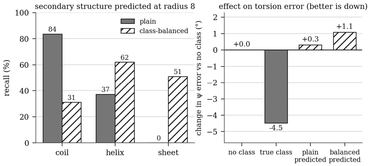
The plain predictor assigns sheet to none of the 82,949 test residues and calls 87.8% of true sheet residues coil; its Q3 of 58.0% is close to what the coil prior alone yields. Class-balancing repairs exactly that deficiency, raising sheet recall from zero to 51.0%, and pays with coil, which is 55% of residues: overall error rises from 42.0% to 56.3%, past the point at which the corruption sweep says the channel is worthless.
Table 7.
Torsion error using predicted rather than true classes, matched seed.
| torsion | seed | base | plain predicted | balanced predicted |
| φ | 11 | 23.0 | 23.0 | 23.1 |
| φ | 23 | 23.0 | 22.9 | 23.1 |
| ψ | 11 | 47.9 | 48.2 | 48.7 |
| ψ | 23 | 47.5 | 47.9 | 48.9 |
Both are worse than supplying no class at all, and the predictor with the better sheet recall gives the worse torsion model. The oracle result requires correct labels and sheet coverage, and a radius-8 window supplies one or the other.
The plain predictor’s 42% error rate should, by the corruption sweep, be worth roughly −1 to −1.5°; it delivers +0.3°. The discrepancy is informative. Corrupted-oracle errors fall at random, whereas a predictor’s errors fall on the residues that are hard to classify, which are the residues the torsion model already gets wrong. The same mechanism accounts for two other failures reported below, and it should be the default expectation for any two-stage design of this kind rather than a surprise encountered three times.
The structural reason is straightforward. An α-helix’s defining i → i+4 hydrogen bond fits comfortably inside a radius-8 window. A β-strand’s pairing partner is routinely tens of residues distant along the chain, frequently at its far end, and sometimes on a different chain. The class channel is worth 5.9° precisely because it summarises non-local context—which is why a local window cannot reconstruct it.
The Pairing Partner Itself Carries Nothing
If the class channel works because it summarises non-local context, the partner that context refers to should be worth more than the summary. That is testable directly. PDB SHEET records carry explicit registration, so the partner of a strand residue is recoverable from the deposition: 3,464 chains and 66,863 partnered residues, 49.0% of the sheet population. The pairing is emphatically non-local—median separation 25 residues, ninetieth percentile 104, and 86.2% of pairs lie outside radius 8, a fifth outside even the ±64 that recurrence reached.
Table 8.
The β-pairing oracle, three seeds. none is the exact control and reproduces its baseline seed digit for digit.
Table 8.
The β-pairing oracle, three seeds. none is the exact control and reproduces its baseline seed digit for digit.
| torsion | arm | weights | MAE | helix | sheet |
| φ | base | — | 22.94 | 19.39 | 32.52 |
| φ | partner type | 1,584 | 20.76 | 17.96 | 28.30 |
| ψ | base | — | 47.72 | 40.50 | 67.15 |
| ψ | none (control) | 0 | 47.93 | 39.91 | 69.53 |
| ψ | partner present only | 72 | 40.03 | 34.95 | 53.73 |
| ψ | partner type | 1,584 | 40.07 | 34.95 | 53.86 |
Supplying it adds one term to the model, indexed by the partner rather than by any sequence separation, a[i][b] += P[type(partner(i))][l][b]—1,584 weights, and zero-initialised so that epoch 0 is the frozen model exactly.
The gain is large—7.65° on ψ and 13.29° on ψ sheet, exceeding every other intervention in this study. It is also not what it appears to be.
Knowing that a residue has a registered partner is itself secondary-structure information: it says the residue sits in a strand. The present arm collapses all twenty-two type banks into one, so the channel reports only that a partner exists and not which residue it is. It recovers the entire effect with 72 weights. Per seed, ψ is 40.036 / 40.046 / 40.022 for present against 40.046 / 39.992 / 40.180 for type; the matched-seed differences are +0.010, −0.054 and +0.157, with no direction, and the identity-indexed arm is the noisier of the two despite twenty-two times the parameters.
So partner identity contributes nothing, and the channel is the class channel reached by another route—a sharper one, which is why it exceeds 5.9°. Only 49% of sheet residues carry registration, so the flag selects regular, registered β-structure rather than everything the depositor labelled sheet.
Whether a partner could be identified from sequence is a separate question and it also answers negatively. Treating the extracted pairings as labels makes recovery a supervised problem: a content-addressed model given the raw 17-residue windows of both residues, at 47,872 parameters, recovers the partner as its first choice 4.07% of the time on strand-restricted candidates, where a baseline using only the empirical distribution of |i − j| and ignoring residue identity entirely reaches 10.07%. Adding identity to that baseline degrades it monotonically, to 8.85%, 6.66% and 5.24% at increasing weight. Identity is not merely uninformative about which strand pairs with which; the learned scores are fitted noise.
That is the expected result on reflection. β-pairing is backbone hydrogen bonding, and which strands pair is set by the fold’s topology—chain connectivity, loop lengths, burial—rather than by the two residues’ side chains. It is the reason coevolutionary signal identifies contacts and a single sequence does not.
Correlated Error Is a Property of the Input, Not of the Architecture
Every two-stage design in this paper failed for the same reason, and the reason was quoted as a single correlation coefficient. That scalar conflates two causes. Two models may fail on the same residues because they read the same seventeen residues, in which case nothing inside a local window can help; or because they read it through the same architecture and retreat to the same modal basin when unsure, in which case a differently-constrained model would fail elsewhere and could be combined with the first. Only the second leaves anything to exploit.
They separate by measurement. The ceiling on error correlation is not 1.0 but the correlation between two runs of the same model differing only in random seed; any pair of models correlating at that level carries no additional information. Table 9 compares that ceiling against a pair differing in architecture—the per-residue-type model against the convolutional control, same seed, same scored residues.
Table 9.
Pearson correlation of circular absolute error, and the percentage of one model’s worst decile falling in the other’s. Independence would give 10%.
Table 9.
Pearson correlation of circular absolute error, and the percentage of one model’s worst decile falling in the other’s. Independence would give 10%.
| comparison | φ r | φ decile | ψ r | ψ decile |
| same model, different seed (ceiling) | 0.967 | 90.6% | 0.943 | 85.2% |
| convolutional control, different seed | 0.859 | 84.7% | 0.723 | 70.2% |
| per-residue-type against convolutional | 0.871 | 85.8% | 0.749 | 56.0% |
| linear control against the nonlinear model | 0.932 | 91.1% | — | — |
| φ against ψ, same architecture | 0.373 | 27.8% | — | — |
On φ the result is unambiguous and negative. Replacing the architecture entirely—27,000 per-residue-type weights against 116,068 convolutional ones, sharing no constraint—takes the correlation from 0.967 to 0.871, which is higher than the convolutional model’s own seed-to-seed ceiling of 0.859. Changing the whole architecture decorrelates less than changing one random seed. The linear control makes the same point from the other end: removing the nonlinearity altogether leaves 91.1% of the worst decile in common. On the residues where the model is worst, the convolutional control averages 92.2° against 15.1° elsewhere, a ratio of 6.09 where two seeds of the same model give 6.66. It is not a second opinion; it is lost on the same residues.
On ψ there is a little more room—the worst-decile overlap falls to 56.0%—but the correlation of 0.749 sits essentially at the convolutional model’s own seed ceiling of 0.723, so most of the apparent diversity is that model scattering between initialisations rather than architectural difference. This is consistent with the ensemble arm, where seed-averaging the convolutional model alone accounted for most of the gain.
The consequence is general. Within sequence-alone prediction at radius 8, which residues are hard is a property of the input rather than of the model reading it, and no rearrangement of the reader reaches them.
A Reproducibility Floor of Three to Six Degrees
Across the enlarged set, 1,092 pairs exceed 90% ungapped identity, 654 of them at exactly 100%, drawn from 1,146 distinct chains. Because the dataset stores no chain identifier, each chain must be recovered from the deposition by sequence matching; 1,108 of the 1,146 were recovered, leaving 1,069 pairs measurable at full precision and contributing 131,771 scored core positions in φ and 131,380 in ψ. All figures below are over those pairs.
Table 10.
Circular absolute difference between independently deposited structures of near-identical sequence, from coordinates, over helix and sheet positions where both structures define the angle and assign the same residue type. Per-pair values are in the supplementary data.
Table 10.
Circular absolute difference between independently deposited structures of near-identical sequence, from coordinates, over helix and sheet positions where both structures define the angle and assign the same residue type. Per-pair values are in the supplementary data.
| population | pairs | φ mean | φ median | φ p90 | ψ mean | ψ median | ψ p90 |
| all pairs | 1,069 | 5.98 | 3.60 | 12.38 | 5.81 | 3.33 | 11.89 |
| 100% identity only | 641 | 5.80 | 3.47 | 12.16 | 5.66 | 3.21 | 11.72 |
| same space group | 672 | 5.37 | 3.27 | 11.19 | 5.18 | 3.01 | 10.63 |
| different space group | 397 | 7.50 | 4.63 | 15.09 | 7.41 | 4.28 | 14.79 |
| conditions matched | 523 | 5.45 | 3.38 | 11.44 | 5.20 | 3.09 | 10.88 |
| conditions differ | 546 | 6.63 | 3.93 | 13.59 | 6.57 | 3.67 | 13.16 |
Half of all core residues in independently determined structures of the same sequence agree to within 3.6° in φ and 3.3° in ψ. The mean is higher than the median because the distribution has a real tail: about a tenth of core positions differ by more than twelve degrees, and those are genuine conformational differences rather than measurement scatter. Both statistics are reported throughout, because the mean alone overstates typical disagreement and the median alone conceals the tail.
The environmental terms are measurable and small. Crystal packing is the largest: pairs crystallising in different space groups disagree by 2.13° more in φ and 2.23° more in ψ than pairs sharing one. Collection temperature and pH together account for 1.18° in φ and 1.37° in ψ. Ligand state does not register at all—pairs matched apo-to-apo or holo-to-holo agree no better than mismatched pairs, so induced fit is not detectably inflating the floor at this sample size.
Table 11.
Model error against the floor, on the same population. Model figures are the adopted linear-head arm; its medians are multiples of 5° because it emits bin centres.
Table 11.
Model error against the floor, on the same population. Model figures are the adopted linear-head arm; its medians are multiples of 5° because it emits bin centres.
| statistic | floor | model | constant | model ÷ floor | captured | |
| φ | mean | 5.98 | 22.73 | 28.2 | 3.8 | 25% of 22.2° |
| φ | median | 3.60 | 10.0 | — | 2.8 | — |
| φ | p90 | 12.38 | 55.0 | — | 4.4 | — |
| ψ | mean | 5.81 | 46.76 | 66.3 | 8.0 | 32% of 60.5° |
| ψ | median | 3.33 | 15.0 | — | 4.5 | — |
| ψ | p90 | 11.89 | 160.0 | — | 13.5 | — |
The model captures a quarter of the available range in φ and a third in ψ. The remaining three quarters and two thirds is not conformational indeterminacy: independently determined structures of the same sequence place half of these residues within three and a half degrees of one another, so the geometry is reproducible and the model is failing to predict something that is there. The gap is widest where it is hardest to explain away—at the 90th percentile two independent determinations differ by about twelve degrees while the model differs by 55° in φ and 160° in ψ.
What Does Not Help
Ten interventions produced no improvement, and the list is reported because a constraint is located more precisely by what fails than by what succeeds.
Coupling φ and ψ at decode time, using the empirical joint distribution, fails on arithmetic before it fails empirically: the Ramachandran basin structure imposes a gap of roughly 44 nats where the available pointwise mutual information is about 14. Coupling them at the input, by replacing the all-ones state with the other torsion’s codeword, gains 5.0° and 10.6° when supplied the true value and loses 0.3° and 1.0° when supplied a model’s prediction; the two models’ errors correlate at +0.37, for the reason set out above. Replacing the nearest-codeword decoder with a learned 36 → 72 readout gives 24.7° and 49.7°, worse. Unclassifying residues at the ends of helices and sheets, where assignment is least reliable, changes nothing at 15% (+0.0°, +0.1°) and hurts at 30% (+0.2°, +0.2°). Restoring coil to the loss costs 0.8° and 1.1°, confirming the core-only choice. Ensembling with the convolutional control reaches 22.7° and 46.6°, level with the mixing head by a different route. Increasing training data 2.7-fold changes nothing. Depth, width and radius were swept without improvement.
Discussion
A model at the saturation radius, with 27,000 weights, predicts enzyme-core backbone dihedrals to 22.7° in φ and 46.8° in ψ. Against a reproducibility floor of 6.0° and 5.8° in the mean—3.6° and 3.3° at the median—that is a quarter and a third of what is available. The interesting question is what occupies the rest, and the interventions here converge on one answer: information that exists in the chain but not in a local window.
Five independent lines support this. Capacity does not close the gap, and neither does removing the architecture’s constraints wholesale. Reach does not close it either, and recurrence establishes that at constant parameter count, which removes the capacity confound entirely and independently corroborates the companion paper’s saturation result by an entirely different mechanism [1]. The one intervention that does work at scale—supplying secondary structure—works because it imports a summary of non-local context, and the same architecture cannot reconstruct that summary from a local window, failing specifically and completely on β-sheet for a reason that follows from where a strand’s hydrogen-bond partner sits. Supplying that partner directly, from deposition records, reaches the same conclusion by a route that does not pass through the class label at all, and adds a second measurement to it: the partner’s identity is worth nothing even when handed over, and cannot be identified from sequence in any case. Two unrelated interventions each remove three to four degrees of β-sheet error, and combining them removes less than reach alone does, which is what a shared ceiling looks like. And the error-correlation decomposition closes the argument from the model’s side: the residues a local model gets wrong are the same residues under any architecture, so the difficulty belongs to the input.
The floor measurement bears on a broader question. That sequence determines structure, in a given environment, is not in dispute [9], but the residual error of a sequence-based model is sometimes read as evidence of how far determination extends. It cannot be read that way without a floor: error attributable to the same sequence adopting different conformations is not a failure of prediction at all. Here that component is small. Independently deposited structures agree to about six degrees on cores, and the model is three to eight times further away. Whatever else this result says, it says the geometry is reproducible and the information is there to be had—a point in favour of sequence determination rather than against it, reached from a direction that does not usually supply evidence either way.
It bears equally on a claim it cannot support. One might read a local model’s failure as evidence that determination depends on the environment. It does not: the model’s handicap is locality, not surroundings. When a β-strand’s partner lies a hundred residues away in the same molecule, the information the model lacks is sequence. Nothing in this design distinguishes the rest of the chain from the medium around it, because the model is blind to both in the same way. The floor measurement is where an environmental effect would appear, and it can now be quantified rather than bounded: across the crystallographic range sampled here, changing space group moves a core backbone dihedral by about two degrees and changing temperature and pH by rather less, against a model error of 22.7° and 46.8°. Environment is not the residual.
Correlated error deserves emphasis as a methodological finding rather than an incidental one. Three two-stage designs were tried—φ conditioned on predicted ψ, ψ on predicted φ, and both on predicted secondary structure—and all three failed while their oracle versions succeeded by 5 to 11 degrees. In each case the second stage’s errors fall on the residues the first stage already handles badly. An oracle experiment therefore establishes an upper bound only, and the gap between oracle and honest performance is governed by error correlation rather than by the accuracy of the intermediate predictor: at 42% class error the honest arm underperformed a randomly corrupted oracle at the same rate by more than a degree.
The decomposition in Table 9 says how far that generalises, and the answer is further than expected. The natural remedy for correlated error is architectural diversity, and it is unavailable here: two architectures sharing no constraint correlate more tightly on φ than two seeds of one of them. Any design that hopes to rescue a local model with a second local opinion—an ensemble, a two-stage cascade, a coupled joint model—is drawing that opinion from the same exhausted source. This is a stronger statement than the individual failures, because it holds without reference to which second model is chosen.
Limitations
The dataset is enzymes, where the companion measurement is on general proteins [1], so the accuracy figures here are not directly comparable to it and generality beyond enzymes is untested. The architecture is dataset-dependent in a way worth stating plainly: against the convolutional control it is ahead on one dataset examined during development, level on this one, and behind on a third. It is used here as an instrument whose constraints can be removed one at a time, not as a contribution to predictive accuracy, and no claim of the latter is made.
The floor rests on 1,069 pairs drawn from 1,108 chains, and those pairs are not independent: many share a protein family, so effect sizes are better supported than any interval around them would be. Thirty-eight pairs disagree by more than 15° on average, with a maximum of 42°; some are real conformational differences and some may be artefacts of ungapped alignment where an insertion is present, and they have not been individually triaged. A further 38 of the 1,146 chains could not be matched to a deposited chain by sequence and are excluded; there is no reason to expect their exclusion to be informative, but it is not a random sample either.
Every chain is an X-ray structure, so the comparison samples crystal forms and buffers, not membranes, crowded cytosol or pH extremes. The environmental terms reported here—about two degrees for space group, rather less for temperature and pH—constrain the range present in these depositions and say nothing beyond it. Room-temperature structures are 2% of the set, which is too few to treat cryo-cooling as a separately resolved axis.
The three-pass recurrent arms rest on a single seed and carry no conclusion the replicated arms do not also carry. Every other arm reported here has three. The β-pairing oracle covers 49.0% of sheet residues, since only registered strands appear in SHEET records with an anchor; the unpartnered remainder is treated as having no partner rather than excluded, so the reported gain is a lower bound on what complete registration would give. Because the conclusion drawn from it is negative—that partner identity contributes nothing—a lower bound is the conservative direction. Secondary structure is the depositors’ assignment rather than a recomputed one [8], which adds noise to both the conditioning and the prediction results, though not in a direction that would create the sheet failure. Finally, the model is single-sequence, where the accurate predictors cited use evolutionary profiles and predicted contacts [2]; the conclusion is about what a local window contains, not about what is achievable with a richer input.
Figure 1.
The per-residue-type architecture, and where the mixing head is inserted. The architecture. Each residue holds 36 slots, and a layer replaces that state by a combination of its neighbours’ states within radius 8. The weight applied to each contribution is selected by the residue the contribution comes from, and slot b reaches only slot b, so the 36 slots never mix. The dashed line marks the layer-2 output: the base model decodes from there, and the mixing head is the one place in this study where the element-wise rule is relaxed.
Figure 1.
The per-residue-type architecture, and where the mixing head is inserted. The architecture. Each residue holds 36 slots, and a layer replaces that state by a combination of its neighbours’ states within radius 8. The weight applied to each contribution is selected by the residue the contribution comes from, and slot b reaches only slot b, so the 36 slots never mix. The dashed line marks the layer-2 output: the base model decodes from there, and the mixing head is the one place in this study where the element-wise rule is relaxed.
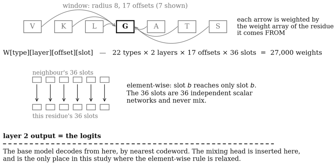
Figure 2.
Mean absolute error against the reproducibility floor, held-out enzyme cores. Mean absolute error against the reproducibility floor, on held-out enzyme cores. Bars are the best constant predictor, the base model, the model with the linear mixing head, per-class models given the true secondary structure, and the floor measured between independently deposited structures of ≥90% sequence identity (dashed line). The distance between the model and the floor is the quantity this paper is about. The floor is measured from coordinates at full precision over 1,092 pairs; its median, 3.6° in φ, is lower still than the mean plotted here.
Figure 2.
Mean absolute error against the reproducibility floor, held-out enzyme cores. Mean absolute error against the reproducibility floor, on held-out enzyme cores. Bars are the best constant predictor, the base model, the model with the linear mixing head, per-class models given the true secondary structure, and the floor measured between independently deposited structures of ≥90% sequence identity (dashed line). The distance between the model and the floor is the quantity this paper is about. The floor is measured from coordinates at full precision over 1,092 pairs; its median, 3.6° in φ, is lower still than the mean plotted here.
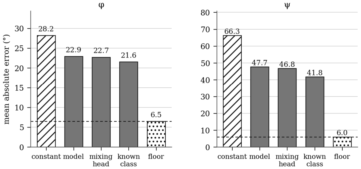
Figure 3.
Recurrence at constant parameter count: ψ error and tail against passes. Recurrence at constant parameter count, ψ, seed 11. Upper panel: mean absolute error against the number of passes through the same 27,000 weights, which multiplies the receptive radius without adding a single parameter, with and without the mixing head. One pass is exactly the base model and reproduces it digit for digit. Lower panel: the ninetieth-percentile error for the headless arm, the only tail movement observed in this study.
Figure 3.
Recurrence at constant parameter count: ψ error and tail against passes. Recurrence at constant parameter count, ψ, seed 11. Upper panel: mean absolute error against the number of passes through the same 27,000 weights, which multiplies the receptive radius without adding a single parameter, with and without the mixing head. One pass is exactly the base model and reproduces it digit for digit. Lower panel: the ninetieth-percentile error for the headless arm, the only tail movement observed in this study.
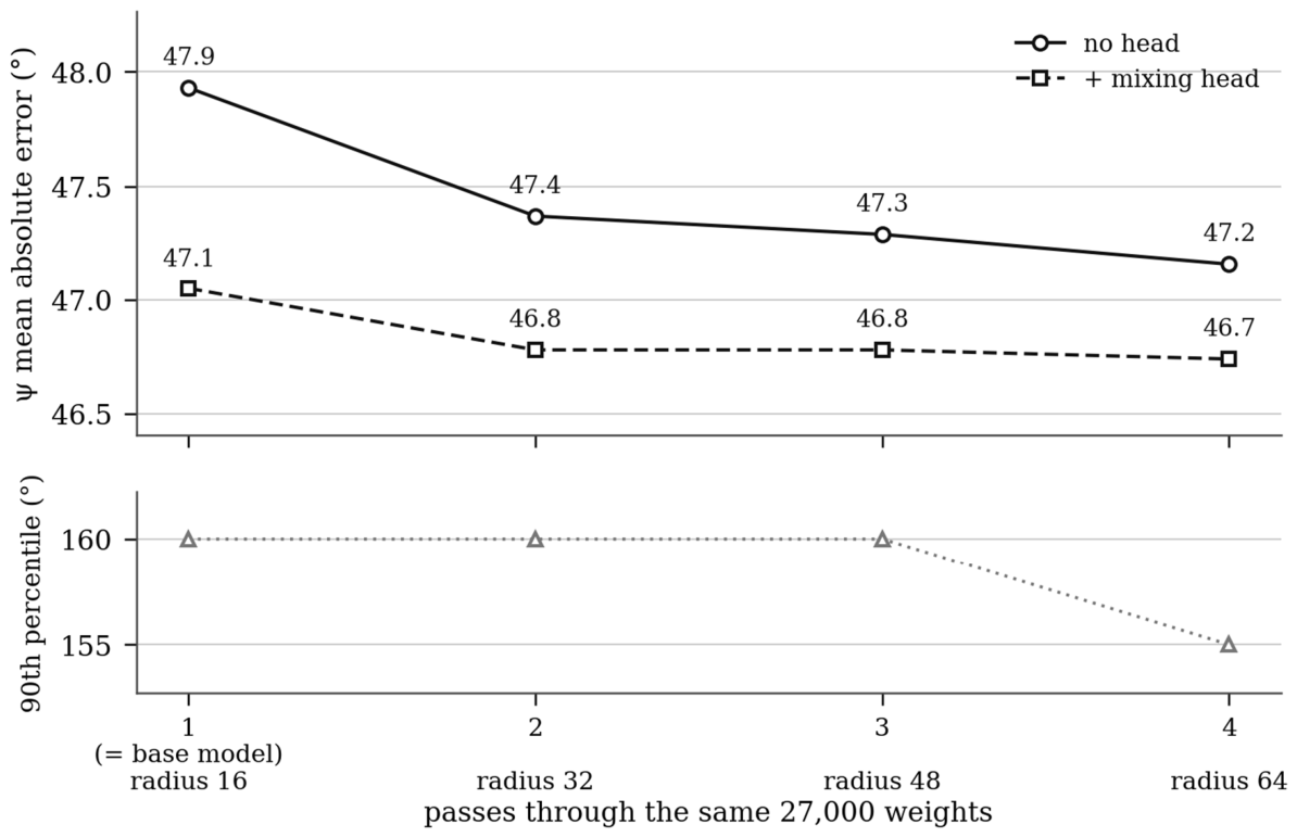
Figure 4.
Per-class recall of the two secondary-structure predictors, and the resulting torsion error. Why the class channel cannot be local. Left, per-class recall on the test split for the plain and class-balanced secondary-structure predictors: the plain predictor assigns sheet to no residue at all, and balancing recovers sheet only by destroying coil. Right, the resulting change in ψ error relative to supplying no class, for the class-as-input form throughout, so the true-class and predicted-class bars differ only in where the class came from. Supplying the true class is worth 4.5°; supplying either predictor’s output is worse than supplying nothing.
Figure 4.
Per-class recall of the two secondary-structure predictors, and the resulting torsion error. Why the class channel cannot be local. Left, per-class recall on the test split for the plain and class-balanced secondary-structure predictors: the plain predictor assigns sheet to no residue at all, and balancing recovers sheet only by destroying coil. Right, the resulting change in ψ error relative to supplying no class, for the class-as-input form throughout, so the true-class and predicted-class bars differ only in where the class came from. Supplying the true class is worth 4.5°; supplying either predictor’s output is worse than supplying nothing.
Author Contributions
Nick Harkiolakis: conceptualisation; methodology; software; formal analysis; investigation; data curation; writing—original draft; writing—review and editing; visualisation.
Funding
This work received no specific grant from any funding agency.
Data Availability Statement
All source code, run scripts, analysis scripts, the prepared datasets and every result file behind this paper are openly available at https://doi.org/10.5281/zenodo.22122427, which resolves to the most recent version of the deposit. This includes the per-pair floor measurements at full precision, the crystallographic metadata table underlying the environmental strata, and the error-correlation decomposition. The structures analysed are public depositions in the Protein Data Bank.
Acknowledgments
Claude (Anthropic) was used in preparing this work: to draft and revise the manuscript text, to write the Python analysis and figure-generation scripts, and to design and script several of the reported controls, including the recurrence formulation and its finite-difference gradient verification of Table 3, the class-balanced secondary-structure predictor of Table 6, and the reproducibility-floor measurement of Table 7. All models were trained and all experiments executed by the author using the released code; every reported value derives from those runs and was verified against the released result files. The author takes full responsibility for the content.:
Conflicts of Interest
The author declares no conflict of interest.:
References
- Harkiolakis, N. How far along the chain is a backbone dihedral written? Saturation radius for φ and ψ. Preprints 2026. [Google Scholar] [CrossRef]
- Hanson, J.; Paliwal, K.; Litfin, T.; Yang, Y.; Zhou, Y. Improving prediction of protein secondary structure, backbone angles, solvent accessibility and contact numbers by using predicted contact maps and an ensemble of recurrent and residual convolutional neural networks. Bioinformatics 2018, 35, 2403–2410. [Google Scholar] [CrossRef] [PubMed]
- Singh, J.; Litfin, T.; Paliwal, K.; Singh, J.; Hanumanthappa, A.K.; Zhou, Y. SPOT-1D-Single: improving the single-sequence-based prediction of protein secondary structure, backbone angles, solvent accessibility and half-sphere exposures using a large training set and ensembled deep learning. Bioinformatics 2021, 37, 3464–3472. [Google Scholar] [CrossRef] [PubMed]
- Swindells, M.B.; MacArthur, M.W.; Thornton, J.M. Intrinsic φ,ψ propensities of amino acids, derived from the coil regions of known structures. Nat. Struct. Mol. Biol. 1995, 2, 596–603. [Google Scholar] [CrossRef] [PubMed]
- Fitzkee, N.C.; Fleming, P.J.; Rose, G.D. The Protein Coil Library: A structural database of nonhelix, nonstrand fragments derived from the PDB. Proteins Struct. Funct. Bioinform. 2005, 58, 852–854. [Google Scholar] [CrossRef] [PubMed]
- Porter, L.L.; Looger, L.L. Extant fold-switching proteins are widespread. Proc. Natl. Acad. Sci. 2018, 115, 5968–5973. [Google Scholar] [CrossRef] [PubMed]
- Berman, H.M.; Westbrook, J.; Feng, Z.; Gilliland, G.; Bhat, T.N.; Weissig, H.; Shindyalov, I.N.; Bourne, P.E. The Protein Data Bank. Nucleic Acids Res. 2000, 28(1), 235–242. [Google Scholar] [CrossRef] [PubMed]
- Kabsch, W.; Sander, C. Dictionary of protein secondary structure: Pattern recognition of hydrogen-bonded and geometrical features. Biopolymers 1983, 22, 2577–2637. [Google Scholar] [CrossRef] [PubMed]
- Anfinsen, C.B. Principles that Govern the Folding of Protein Chains. Science 1973, 181, 223–230. [Google Scholar] [CrossRef] [PubMed]
- Kingma, D.P.; Ba, J. Adam: a method for stochastic optimization. In Proceedings of the 3rd International Conference on Learning Representations (ICLR), 2015. [Google Scholar]
Disclaimer/Publisher’s Note: The statements, opinions and data contained in all publications are solely those of the individual author(s) and contributor(s) and not of MDPI and/or the editor(s). MDPI and/or the editor(s) disclaim responsibility for any injury to people or property resulting from any ideas, methods, instructions or products referred to in the content. |
© 2026 by the authors. Licensee MDPI, Basel, Switzerland. This article is an open access article distributed under the terms and conditions of the Creative Commons Attribution (CC BY) license (http://creativecommons.org/licenses/by/4.0/).
Copyright: This open access article is published under a Creative Commons CC BY 4.0 license, which permit the free download, distribution, and reuse, provided that the author and preprint are cited in any reuse.