

Submitted:
07 September 2026
Posted:
07 September 2026
You are already at the latest version
Abstract
Telemetry data provide essential information on a spacecraft’s in-orbit operating state and its evolution, supporting system health-state awareness, assessment, and judgment. However, existing data-driven health-state modeling methods may provide unstable representations of healthy operating patterns and have difficulty distinguishing local disturbances from state deviations in complex spacecraft telemetry. To address these problems, this paper proposes a Health Prototype Memory Transformer (HPM-Former) for telemetry health-state baseline modeling. HPM-Former uses convolutional structures to extract local fluctuation features and a Transformer to model global temporal dependencies among multivariate telemetry parameters. Health-memory prototypes learn representative healthy patterns under normal operating conditions, enabling stable representations of healthy spacecraft operation. A health-consistency deviation is constructed from reconstruction deviation, health-prototype matching, and uncertainty in memory addressing to characterize input deviation from the health-state baseline, thereby supporting comprehensive state assessment. Experiments on the European Space Agency Anomalies Dataset (ESA-AD) show that HPM-Former stably represents healthy operating patterns and improves the reliability of current-state assessment against the health-state baseline. It outperforms the comparison methods in corrected event-wise F0.5 and event-wise alarming precision, providing an effective data-driven approach for operational-state assessment of complex spacecraft.
Keywords:
spacecraft telemetry
; health-state prototype memory
; Transformer
; multivariate time series
1. Introduction
Complex spacecraft, such as manned spacecraft and deep-space explorers, continuously generate large-scale, high-dimensional, and structurally complex telemetry during long-term on-orbit operations. Telemetry is a primary source of information on a spacecraft’s on-orbit operational state and its evolution, and it uniquely captures the intrinsic operating patterns and fundamental characteristics of the spacecraft [1]. Continuous telemetry monitoring and analysis support real-time awareness of spacecraft operational states, early identification of anomaly-related risks, and mission-control operations. Therefore, extracting representative operating patterns from historical telemetry and constructing a health-state baseline that characterizes nominal system behavior is essential for state awareness and operational assessment of complex spacecraft systems.
Out-of-limits(OOL) alarm and expert-rule methods are widely used in engineering practice because they are simple and interpretable [2]. However, their dependence on historical experience, high manual-analysis burden, and limited ability to update rule bases as spacecraft operational states change have restricted their use in health assessment [3,4]. Data-driven health-state baseline modeling has therefore attracted increasing attention [5,6,7,8]. These methods use the mathematical relationships in historical telemetry to learn healthy operating patterns through machine-learning and deep-learning techniques, and compare the resulting baseline with current telemetry for system health assessment. In this context, health-state baseline modeling establishes a reference of nominal operation, while anomaly detection evaluates deviations from this reference.
Among data-driven approaches, deep-learning-based health-state baseline models have shown higher accuracy and better generalization [9,10,11]. These methods learn the temporal evolution and characteristics of nominal operation from historical healthy telemetry and use prediction values, reconstructions, or latent representations to quantify deviations from the health baseline. Researchers at the Jet Propulsion Laboratory of the National Aeronautics and Space Administration (NASA) used a Long Short-Term Memory (LSTM) network to predict spacecraft telemetry and identified anomalous states through nonparametric dynamic thresholding of prediction errors [12], and the European Space Agency (ESA) later included this approach in its anomaly-detection benchmark [13]. NASA’s data science group proposed a variational autoencoder (VAE)-based model that learns the distribution of nominal operation in latent space and detects state deviations from reconstruction errors [14]. Yan et al. [15] combined K-means clustering with a variational encoder to model the probability distribution of healthy telemetry under different operating modes. Jiang et al. [16] combined a Transformer with LSTM to model global variation patterns and local temporal dependencies, while Zhao et al. [17] proposed the Seasonal Decomposition Cross-Attention Transformer (SDCA-Former) for non-stationary satellite telemetry. The Korea Aerospace Research Institute (KARI) combined multivariate convolutional LSTM with mixtures of probabilistic principal component analysis (PCA) for spacecraft telemetry state monitoring [18], and Liu et al. [9] used temporal convolution and dynamic graph attention to model dependencies among variables and across time.
Despite recent progress, telemetry-based health-state baseline modeling still faces several practical challenges. Prediction-based and reconstruction-based deep learning models generally establish health-state baselines by learning temporal patterns from historical healthy telemetry. However, healthy spacecraft operation inherently exhibits a certain range of variation, and its characteristics may differ across operating conditions. Accurately characterizing healthy states and their normal variation boundaries therefore remains difficult. On the one hand, some telemetry data that have already deviated from healthy operation may still exhibit temporal patterns and inter-parameter relationships similar to those of healthy data over certain time intervals. Such data may still be predicted or reconstructed accurately, making the learned health baseline less distinguishable from these off-nominal states [19]. On the other hand, normal variations caused by operating-condition adjustments, short-term disturbances, or measurement noise may deviate from the typical health patterns learned by the model. As a result, some valid healthy states may not be adequately covered by the established health baseline [20]. Therefore, telemetry-based health-state baseline modeling should not only capture the temporal patterns of nominal telemetry sequences, but also accurately represent typical healthy operating patterns and their normal variation ranges [21,22]. A key challenge is to enhance the model’s representation and memory of healthy patterns, thereby establishing a health-state baseline that adequately covers normal operational variations while remaining well separated from off-nominal states.
To address these challenges, we propose the Health Prototype Memory Transformer (HPM-Former). The model combines Transformer-based temporal modeling with convolutional feature extraction to capture long-term evolution and local variations in telemetry. A health-state prototype memory learns representative healthy operating patterns in latent space, while sparse memory addressing constrains reconstruction to relevant health prototypes, thereby establishing a health-state baseline, reducing over-generalized reconstruction of anomalous structures, and improving separability between healthy and off-nominal states. For operational-state assessment, we further construct a health-consistency deviation score from health-prototype matching, the residual between the query and memory representation, and memory-addressing uncertainty. Reconstruction-error and health-consistency thresholds are calibrated separately from nominal validation data and combined in a joint decision rule, with anomaly risk identified only when both deviations are significant.
The main contributions of this study are summarized as follows: (1) a health-state prototype memory is introduced to learn representative healthy operating patterns and establish a stable health-state reference, while sparse prototype addressing constrains reconstruction to the learned healthy patterns; (2) a health-consistency deviation is constructed from health-prototype matching, the residual between the query and memory representation, and memory-addressing uncertainty, providing state-consistency evidence in addition to reconstruction deviation; and (3) reconstruction deviation and health-consistency deviation are combined in a joint decision mechanism to reduce state misclassification caused by relying solely on model-output error. Experiments on ESA’s public satellite telemetry anomaly-detection dataset demonstrate the effectiveness of HPM-Former in health-state baseline modeling, showing that the established baseline can effectively distinguish healthy operating patterns from abnormal state deviations while maintaining a favorable balance between false-alarm control and anomaly-recognition capability.
2. HPM-Former Model
2.1. Overall Architecture of HPM-Former
The overall architecture of HPM-Former is shown in Figure 1. It consists of an input-representation module, a temporal feature-extraction module, a health-state prototype memory module, a reconstruction-output module, and a health-consistency evaluation module. First, the input telemetry sequence is transformed by feature embedding and positional encoding into a sequence representation that preserves temporal order. The representation is then passed to a fused feature extractor composed of a Transformer temporal-modeling unit and a convolutional local-feature extractor. The Transformer learns global temporal dependencies and trend evolution in the telemetry sequence, while the convolutional structure captures short-term fluctuations and local changes. Together, they produce a latent representation of the telemetry state.
From the latent representation, the model generates a query vector and matches it against learnable health prototypes in the health-state prototype memory. Sparse addressing produces prototype-access weights, and the health prototypes most relevant to the current telemetry state are selected and combined to form a memory-augmented representation. This representation is passed to the reconstruction-output module to generate the reconstructed telemetry sequence. In parallel, the model constructs a health-consistency measure from the input sequence and its latent representation to assess how closely the current telemetry state matches nominal operating patterns. HPM-Former therefore outputs both the reconstructed telemetry and the health-consistency measure, providing complementary reconstruction-error and state-consistency evidence for subsequent health-state deviation assessment.
During training, sustained-offset samples are generated from the original telemetry training data as references outside the health-state boundary. Specifically, channels and continuous segments are randomly selected from healthy telemetry windows. A fixed offset matched to the normal fluctuation scale of the selected channel is then added to simulate a persistent state deviation. This enables the model to learn healthy operating patterns while defining the valid range of the health-state baseline.
2.2. Telemetry Input Representation
Spacecraft telemetry typically consists of multiple continuously sampled physical quantities. Different telemetry channels can differ substantially in units, value ranges, variation rates, and noise levels. For a given multivariate telemetry window, the model must represent the multichannel state at each sampling instant while preserving temporal order. HPM-Former therefore first applies a temporal representation module that maps the raw telemetry window to a common-dimensional latent sequence representation and adds positional encoding to retain temporal-location information within the window.
Let the input telemetry window be , where T is the window length, C is the number of telemetry channels, and is the multichannel telemetry observation at sampling instant t. To map observations from different channels into a common feature space, a linear embedding layer is applied to the telemetry vector at each time step:
where is the input embedding matrix, is the bias term, d is the latent feature dimension, and is the embedding at time step t. Arranging the embeddings in temporal order gives . This operation maps the original C-dimensional channel vector at each time step to a d-dimensional representation, allowing the convolution, attention, and memory modules to operate in a unified latent space.
The embedded representation E mainly describes the multivariate state at each time step but does not explicitly encode its temporal position within the window. Because telemetry health states usually evolve over time, the model further introduces learnable positional encoding. The positional-encoding matrix is defined as:
where denotes the positional vector at time step t. Unlike fixed sinusoidal positional encoding, the positional vectors are trainable model parameters and can adapt to the telemetry-window modeling task. The input embedding and positional encoding are added element-wise to obtain the output of the temporal representation module, . This representation incorporates temporal-position information and provides a common input to subsequent feature extraction and fusion.
2.3. Temporal Feature Extraction and Fusion
After the latent representation is obtained, the model extracts deeper features that characterize changes in the telemetry state. Spacecraft telemetry states exhibit different variation characteristics across multiple time scales. Local fluctuations over short periods reflect the transient responses of telemetry parameters, whereas long-term trends represent state evolution and contextual relationships. Based on this characteristic, HPM-Former fuses local convolutional features with global temporal features extracted by the Transformer. It therefore forms an operational-state representation that captures both local variations and overall evolution within the same latent space.
2.3.1. Local Feature Extraction by Convolution
The convolutional local-feature extractor captures short-term variation patterns between adjacent temporal positions. A one-dimensional convolution slides along the time axis and aggregates local-neighborhood information without disrupting temporal order. As a result, the latent representation at each time step contains variation features from both the current and neighboring time steps.
The model uses two one-dimensional convolutional layers, each followed by a Gaussian Error Linear Unit (GELU) activation. The computation is given by:
where denote the outputs of the first and second convolutional layers, respectively. The GELU activation introduces nonlinear representation capability and is defined as , where is the cumulative distribution function of the standard normal distribution. Compared with hard-threshold activation functions, GELU is smoother around zero and better preserves the influence of small state variations on subsequent feature extraction. Early health-state deviation in spacecraft telemetry may not appear as a large limit violation; instead, it can manifest as a small but persistent change. The smooth activation therefore helps preserve subtle local variations that carry state information. Through the two convolutional layers, the initial temporal representation is transformed into the local temporal feature , which provides a locally enriched input to subsequent Transformer-based temporal modeling.
2.3.2. Transformer-Based Temporal Modeling
Convolutional features are mainly based on local neighborhoods and cannot fully describe the overall correlation between different temporal positions within the current window. Based on the local temporal feature , this paper introduces the Transformer temporal modeling unit. Through the self-attention mechanism, it calculates the correlation between time positions within the window, reorganizes these local features, and enables the model to highlight the time positions and key change information that contribute more to the representation of the current state, forming an overall correlation of trend-enhanced features .
The Transformer temporal-modeling unit consists mainly of multi-head self-attention, layer normalization, residual connections, and a feed-forward network. HPM-Former uses a pre-layer-normalization (Pre-LN) architecture, in which layer normalization is applied before the multi-head self-attention and feed-forward sublayers. This improves the scale stability of features entering each sublayer. The input features are first normalized to reduce scale differences among latent features at different temporal positions, yielding the normalized temporal representation Z. Z is then projected into the query matrix Q, key matrix K, and value matrix V.
, , and are the corresponding linear-projection parameters. Q and K are used to compute correlations among temporal positions, while V contains the temporal features to be aggregated. The attention output is defined as:
where is the feature dimension of a single attention head. Each temporal position can thus aggregate information from other positions according to their relevance. Unlike convolution, which mainly depends on local neighborhoods, self-attention directly connects arbitrary positions in the sequence and is therefore well suited to modeling global relationships and complex temporal dependencies in telemetry.
Multi-head self-attention further extracts temporal relationships from different feature subspaces. The outputs of all attention heads are concatenated and linearly transformed to obtain the multi-head attention output:
where h is the number of attention heads and is the output projection matrix. Concatenating and transforming the heads allows the model to integrate relationships learned in different subspaces and obtain the multi-head attention feature A. The attention output is then added to the input through a residual connection. This preserves the original local temporal features and reduces the risk of losing convolution-derived local variations during the attention transformation. Dropout is used to reduce over-reliance on specific transformed features and improve robustness. A feed-forward network then performs a nonlinear transformation at each temporal position. With the residual connection, the Transformer unit outputs . This representation integrates global sequence relationships and complex temporal context while retaining the local variation information contained in .
2.3.3. Gated Residual Fusion
The final temporal latent representation is generated through learnable residual injection of Transformer-derived trend features. is used as the local-trend representation, and serves as a trend-correction term. A learnable gate controls the strength of this correction. Let G be a gating matrix with the same dimensions as , where . The fused representation is:
where is an all-ones matrix of size , ⊙ denotes element-wise multiplication, and is a learnable scalar gating coefficient. At the beginning of training, can be initialized to a small value so that the model first retains the stable convolutional representation. As training proceeds, adapts to the optimization objective and determines the contribution of Transformer-derived temporal information to the final latent representation.
2.4. Health-State Prototype Memory
After the temporal feature-extraction and fusion module produces H, a health-state prototype memory module is introduced to store and retrieve representative health-state patterns in latent space. Healthy spacecraft operation is rarely represented by a single fixed pattern; instead, it includes multiple typical operating modes. If reconstruction relies only on the current window’s latent representation, the model may generalize strongly to locally off-nominal segments, reducing the reconstruction contrast between healthy and off-nominal states. We therefore introduce a health-state prototype memory matrix in latent space and represent healthy operating patterns as a set of addressable prototypes. Similarity matching and sparse combination generate a memory-augmented representation that constrains subsequent reconstruction, thereby improving separability between healthy and off-nominal states, as shown in Figure 2.
The core of the health-state prototype memory is a learnable matrix . N denotes the number of health prototypes, and the j-th row of M is denoted by , representing the j-th health-state prototype. The memory matrix M is randomly initialized at the beginning of training. It is jointly optimized with the other model parameters. During training, nominal telemetry windows are mapped into the latent space and used to update the corresponding memory items. The reconstruction objective drives these memory items to retain representative characteristics of normal spacecraft operating states. As a result, the memory matrix gradually forms a set of health-state prototypes covering different nominal operating modes. Instead of reconstructing directly from the input-window representation, the model first generates a query vector for the current window, uses the query to address the health-state prototype memory, and then combines the selected prototypes by weighted summation to obtain a memory-augmented representation.
2.4.1. Query Vector Generation
Memory addressing requires a sample-level query vector that summarizes the overall state of the current telemetry window. We construct the query from both the window-center state and latent-space variation statistics. The latent feature at the center of the window represents its dominant state, while statistics of differences between adjacent time steps capture the strength of within-window changes. Let the center position be , with , and define the base-state vector as . To characterize within-window variation, the latent difference between adjacent temporal positions is computed as . Statistical pooling is then applied to to obtain the variation-statistics vector:
where mean, std, and max denote the mean, standard deviation, and maximum value statistics, respectively, and perform global statistics on both the time dimension and the latent space feature dimension. represents the center state of the current window, whereas characterizes the magnitude of within-window variation. They describe the latent state of the telemetry window from complementary perspectives. The two vectors are concatenated, linearly projected, and layer-normalized to obtain the query vector for memory addressing:
where and are the query-projection parameters, denotes layer normalization, and is the query vector for the current telemetry window. Because the query combines the center state with latent variation statistics, it more effectively represents how the current window should be matched in the health-state prototype space.
2.4.2. Health-State Prototype Memory Addressing
Given the query vector q, the model evaluates the match between the current telemetry window and each health prototype in memory matrix M. Because q and all prototypes lie in the same latent space, cosine similarity is used to measure their proximity. The similarity to the j-th prototype is defined as:
where denotes the similarity between query q and health prototype , and is the norm. The similarities for all prototypes form the vector . To convert similarity values into access weights for prototype retrieval, temperature scaling and Softmax are applied:
where is the temperature coefficient and is the vector of prototype-access weights. A larger indicates that the j-th health prototype is more relevant to the current window and therefore receives a higher weight during memory retrieval.
The access weights obtained solely using Softmax are typically dense, with multiple prototypes participating in the representation with relatively small weights. In a health-state prototype memory, an overly dense combination can reduce prototype selectivity and allow the current window to be explained by too many prototypes. To improve the discriminative capability of memory addressing, the access weights are sparsified. Small weights are suppressed to zero or near zero, leaving only the most relevant prototypes. The sparsification operation is:
where is the sparsity threshold and denotes the threshold-shrunk access weights. ReLU sets weights below to zero and retains only values above the threshold. The nonzero weights are then normalized:
is the sparse access weight for the j-th prototype. If threshold shrinkage removes all valid prototypes, a Top-k fallback strategy retains the k largest Softmax weights to ensure stable memory retrieval. This sparse addressing mechanism allows the model to prioritize a small set of health prototypes most relevant to the current state rather than averaging over the entire memory matrix.
After the sparse access weights are obtained, the model performs a weighted read from the health-state prototype memory matrix M to generate the memory-augmented representation:
Because has large values only for a small number of relevant prototypes, is mainly composed of health prototypes close to the current telemetry state. Thus, before entering the reconstruction-output module, the latent state of the input window is mapped into the representation space spanned by the health-state prototype memory. For a window consistent with nominal operation, the query can find nearby health prototypes and preserve its state characteristics well. For a window that deviates from nominal patterns, the query is difficult to represent adequately with a small number of health prototypes, so the subsequent reconstruction is more likely to differ from the original input. The resulting memory representation is .
2.5. Reconstruction Output and Health-Consistency Evaluation
2.5.1. Prototype-Constrained Reconstruction
After the memory-augmented representation is obtained, a decoder maps it back to the original telemetry-sequence space to generate the reconstruction. Because is a sample-level latent vector and does not directly correspond to a telemetry sequence of length T, the decoder first maps it to an initial reconstruction feature . is then repeated T times along the temporal dimension and combined with decoder positional encoding to obtain a length-T latent reconstruction sequence . Two one-dimensional convolutional layers unfold and locally reorganize the sequence features, producing the decoder feature . Finally, a linear output layer maps the latent features back to the original telemetry-parameter space:
where denotes the reconstructed telemetry window generated by the decoder, and and are the output-layer parameters. Because the decoder input is a sparse combination of health-state prototypes, the reconstruction is constrained by the learned health-prototype representation. When the input window follows nominal operating patterns, provides an effective healthy-state representation and the decoder can reconstruct the original input closely. When the input contains structures that deviate from the health pattern, cannot fully represent those structures and the reconstruction error increases. The prototype-based representation used by the decoder remains . For an original input window X, the point-wise reconstruction error is therefore defined as:
2.5.2. Modeling the Health-Consistency Deviation
Using reconstruction error alone to measure the difference between the current state and the health-state baseline is susceptible to local noise and short-term disturbances. It is also difficult to use reconstruction error to represent smooth state deviations continuously. To address this limitation, a health-consistency deviation is constructed from the health-state prototype memory. It evaluates the consistency between the current window and representative healthy operating patterns according to their matching relationships in the latent space.
If the current window is nominal, its query vector usually forms a stable match with the health prototypes and the difference between q and remains small. If the window deviates from a healthy state, prototype matching may weaken, memory-addressing uncertainty may increase, or the difference between the query and memory representation may become larger. Based on these observations, we construct features describing memory-matching deviation and addressing uncertainty.
The memory-residual feature is ; the degree of prototype mismatch is ; and the dispersion of memory-addressing weights is characterized by the attention entropy . These features are defined as follows:
The health-consistency feature vector of the current window is therefore:
To avoid excessive sensitivity of a single memory-feature threshold to complex nominal conditions, we estimate the statistical distribution of the health-consistency features from nominal validation windows. Let the set of health-consistency features in the nominal validation set be . The mean vector and covariance matrix are then defined as:
To improve numerical stability when inverting the covariance matrix, a diagonal regularization term is added:
The health-consistency deviation of the current window is finally defined as the squared Mahalanobis distance of the health-consistency feature from the nominal healthy distribution:
where . A small indicates that the memory-matching relationship of the current window is close to that of nominal healthy windows. A large indicates deviation from the nominal distribution in health-prototype matching or memory-addressing uncertainty and therefore a higher likelihood of an abnormal health state. This modeling approach complements reconstruction deviation by evaluating the consistency of healthy patterns in the latent space. It provides a basis for quantitatively assessing the current state against the health-state baseline.
2.5.3. Joint Assessment of Reconstruction Deviation and Health Consistency
The reconstruction output module and the health-consistency deviation characterize observation-level deviations and latent-space deviations from healthy patterns, respectively. The two continuous quantities are jointly calibrated to produce a comprehensive assessment of the current window against the health-state baseline. Because telemetry channels differ in their measurement scales and normal fluctuation ranges, the reconstruction residual of each channel is first calibrated using the healthy validation set. Let the reconstruction-residual threshold of channel j be . The normalized reconstruction residual is:
To emphasize meaningful channel deviations within a window while reducing the influence of extreme values at isolated samples, we first take the maximum normalized residual across channels at each time step and then compute a high-quantile statistic over the window. The resulting window-level reconstruction-deviation score is:
where denotes the 95th percentile. If , the window contains a reconstruction deviation beyond the residual range observed in the nominal validation set.
The health-consistency deviation , computed as a squared Mahalanobis distance from the nominal health distribution, is a continuous deviation score. A health-deviation threshold is calibrated from the nominal validation set, yielding the normalized health-deviation score:
The corresponding reconstruction-deviation decision, health-consistency decision, and final joint decision are:
where is the indicator function, equal to 1 when the condition is satisfied and 0 otherwise.
2.5.4. Module Constraints and Loss Design
The primary objective of the health-state prototype memory module is to learn representative and discriminative health-state prototypes in memory matrix M, so that the reconstruction process preferentially relies on these prototypes for state representation. To achieve this objective, the module is trained with the following constraints.
(1) Nominal reconstruction constraint. Healthy telemetry windows should be reconstructed accurately after prototype addressing and memory augmentation. This encourages the health-state prototypes to cover the main patterns of nominal operation and ensures that retains sufficient health-state information. (2) Prototype-structure constraint. Prototype diversity, memory-addressing entropy, and prototype-usage constraints are used to prevent excessive similarity among prototypes, over-concentration of access weights, and long-term inactivity of some prototypes. These constraints promote a stable and well-dispersed health-state representation in the memory matrix. (3) Health-feature separability constraint. Because the health-consistency deviation is computed from the Mahalanobis distance of memory-matching features from the nominal health distribution, the deviation score is not directly supervised as a binary probability during training. Instead, the underlying memory-feature space is constrained. Memory features of nominal windows are pulled toward the health-feature center, while those of off-nominal windows are pushed away. A ranking constraint further increases the separation between nominal and off-nominal windows in memory-feature space, improving the discriminative capability of the subsequent Mahalanobis-distance-based health-consistency deviation.
Combining these constraints, the overall training loss is:
where is the nominal reconstruction constraint, which ensures that healthy telemetry windows can be accurately reconstructed through the health-prototype memory; is the prototype-structure constraint, which improves prototype discrimination and regularizes memory addressing and prototype usage; is the health-feature separability constraint, which increases the distance between nominal and off-nominal windows in memory-feature space and improves the discriminative capability of the health-consistency deviation; and and are the corresponding weighting coefficients. With these constraints, the model jointly learns reconstructable nominal patterns, a stable health-prototype structure, and feature-level separation between healthy and off-nominal states, thereby improving the identification of telemetry health-state deviations.
3. Experimental Validation, Results and Discussion
3.1. Experimental Setup
1) Dataset
Experiments are conducted on ESA-AD, a public benchmark for satellite telemetry anomaly detection. The data originate from real in-orbit ESA satellite missions and include multivariate telemetry channels, anomaly events, and communication gaps. The events were manually annotated by spacecraft operations engineers and machine-learning experts and cross-verified using state-of-the-art algorithms. Compared with commonly used public datasets such as NASA Soil Moisture Active Passive (SMAP) and Mars Science Laboratory (MSL), the ESA Anomaly Detection Benchmark (ESA-ADB) places greater emphasis on the complexity of real space-mission telemetry, including multichannel coupling, changes in sampling frequency, long-term operating-mode drift, and anomalous samples in the training data. It therefore more closely reflects practical satellite health-monitoring scenarios. Because ESA-AD is derived from operational satellite missions, mission names, channel semantics, the true timeline, and some mission-related information are anonymized. We therefore use the anonymous channel identifiers provided by the dataset rather than assigning physical names to the selected channels.
ESA-ADB contains two missions for benchmark evaluation. Mission 1 has 76 telemetry channels, including 58 target channels and 18 non-target channels. Mission 2 has 100 telemetry channels, including 47 target channels and 53 non-target channels. In addition to the full-channel benchmark settings, ESA-ADB provides a lightweight channel subset. For Mission 1, subsystem 5 contains six telemetry channels, Channels 41–46. This subset preserves joint variations across multiple telemetry channels and channel-level anomaly annotations at a smaller input scale. We use this setting so that the model input retains joint variations among related telemetry channels while avoiding interference from large numbers of irrelevant and non-target channels. This makes the subset suitable for analyzing the key mechanisms of HPM-Former, including temporal feature extraction, health-state prototype memory, and health-consistency evaluation. Nine months of data, totaling 901,206 data points, are used for training and validation with an 8:2 split. Four months of data, totaling 418,800 data points, are used for testing, with an anomaly rate of 1.58%.
2) Data Preprocessing
The raw telemetry is irregularly sampled and contains heterogeneous channel types. To remain consistent with the official ESA-AD benchmark procedure and facilitate comparison with ESA baselines such as the ESA-adapted dilated-convolutional variational autoencoder (DC-VAE-ESA) and Telemanom-ESA, we follow the benchmark’s basic preprocessing strategy. The telemetry is time-aligned, standardized by channel, and partitioned into samples.
The Mission 1 telemetry is first resampled to a common 30-s interval. Each telemetry channel is resampled using zero-order hold, which carries the latest known value forward to each new sampling instant. Let the original observation times be and the resampled time points be . Zero-order hold is defined as:
Unlike linear interpolation, zero-order hold does not create artificial intermediate states between two actual samples. It is therefore better suited to state variables, quantized measurements, and discontinuously changing signals commonly found in satellite telemetry.
Telemetry channels differ in amplitude range and fluctuation scale. Without normalization, channels with larger amplitudes may dominate the reconstruction error and gradient updates. We therefore standardize each channel separately to reduce the influence of unit and scale differences on model training and anomaly scoring:
where and are the mean and standard deviation of channel c computed from the training set. To convert the continuous multivariate telemetry into model inputs, the standardized sequence is segmented with a sliding window. Let the standardized multivariate sequence be X = {{, , …, }}. A local window of length T is used to construct each sample. The i-th window is , written as , where ; S is the stride. We set T = 250 and S = 25, producing a sequence of overlapping window samples. The same windowing procedure is applied to the training, validation, and test sets.
3) Model Parameter Settings
HPM-Former is implemented in TensorFlow 2.5.1 with CUDA 11.0. Training and detection are performed in a Docker container with Python 3.6.9, NumPy 1.19.5, and Pandas 1.1.5. Computation uses one NVIDIA GeForce RTX 4060 Ti GPU with 8 GB of memory. The host system is Windows 10 Pro with a 12th Gen Intel Core i5-12400F CPU. All experiments use the same software environment and random seed (seed = 42). The main model parameters are listed in Table 1.
Each training batch contains nominal windows and synthetically generated anomalous windows. Nominal windows are used to learn reconstructable baseline states, while anomalous windows provide contrasting examples of off-nominal states. During training, a contiguous segment of length 25 is randomly masked in each input window. The masked window is fed to the model, while the original unmasked window remains the reconstruction target. For nominal windows, the loss primarily optimizes reconstruction over the masked region, with a lower-weight full-window reconstruction term. Anomalous windows are used to increase the health-deviation score of off-nominal states and reduce the likelihood that they are explained with high confidence by health prototypes. Memory matrix M is updated end-to-end. Prototypes that are effectively accessed by nominal windows and help reduce reconstruction error receive the main gradient updates. Memory-diversity, access-entropy, and prototype-usage constraints prevent memory collapse and persistent reliance on only a few prototypes. Gradient clipping is used to stabilize training.
The validation stage is used for model selection and baseline calibration. The reference ranges are determined from the reconstruction deviations and health-consistency deviations of the healthy validation windows. During testing, the model parameters and calibration results remain fixed, and the two deviations are calculated for each window in the test sequence. A window is recorded as a significant state deviation when both quantities exceed their respective health reference ranges. These results are subsequently used for event-level evaluation. Test labels are used only to calculate the evaluation metrics and do not participate in model training or baseline calibration.
3.2. Evaluation Metrics
ESA noted that, for health-state baseline modeling, evaluation should not be limited to whether individual time points are identified as anomalous. It should also examine whether the model can respond effectively to a complete state-deviation process and provide assessment results suitable for engineering analysis. Point-wise metrics alone cannot adequately determine whether a state-deviation event is identified, whether numerous redundant alarms are generated, whether the affected channels are correctly localized, or whether the response timing is appropriate. Therefore, this study adopts the hierarchical evaluation metrics proposed by ESA-ADB to evaluate the effectiveness of the constructed health-state baseline and the resulting state assessment in terms of event identification, false-alarm control, channel localization, alarm redundancy, and anomaly-interval matching.
(1) Corrected event-wise F0.5-score. This metric evaluates overall state deviation. Let , , and denote event-wise true positives, false positives, and false negatives, respectively. Let be the duration of normal operation correctly classified as normal and be the total duration of normal operation. Corrected event-wise precision, event-wise recall, and the corrected event-wise F0.5-score are defined as:
F0.5 places more emphasis on precision compared to F1, making it suitable for scenarios where there are stringent requirements for false positive control.
(2) Channel-aware F0.5-score. This metric evaluates whether the model correctly localizes the telemetry channels affected by an anomaly. Let , , and denote channel-level true positives, false positives, and false negatives, respectively. Then:
(3) Event-wise alarming precision. This metric evaluates whether alarms are redundant or invalid and is computed as:
where is the number of valid alarms associated with real anomaly events and is the total number of alarms generated by the model.
(4) Anomaly detection timing quality curve (ADTQC). This metric evaluates the agreement between the detected start time and the true anomaly start time. Let denote the start-time difference for the k-th correctly detected event. Then:
where is the timing-quality function defined by ESA-ADB and is the number of correctly detected anomaly events. This metric measures whether an anomaly is detected within a reasonable time range.
(5) Modified affiliation-based F0.5-score. This metric evaluates the affiliation between predicted anomalous intervals and ground-truth anomalous intervals. Let and denote affiliation-based precision and recall, respectively. Then:
3.3. Experimental Results and Discussion
To evaluate HPM-Former for spacecraft telemetry anomaly detection, we compare it with three representative types of methods from ESA-ADB using the same test data and evaluation metrics. The comparison methods are: (1) DC-VAE-STD3/STD5, a multivariate reconstruction method based on a dilated-convolutional variational autoencoder. Dilated convolutions capture short- and long-range temporal dependencies, and an anomaly is flagged when the deviation between measured and reconstructed telemetry exceeds 3 or 5 standard deviations. (2) Global-STD3/STD5, a global statistical threshold method. A nominal range is established from the mean and standard deviation of each training channel, and samples beyond the 3 or 5 threshold are classified as anomalous. (3) Telemanom-ESA, an LSTM-based predictive anomaly detector. It uses historical multichannel telemetry to predict the future state of a target channel and combines prediction error with a nonparametric dynamic threshold to identify anomalies.
These methods are selected for three reasons. First, they are representative methods used in the official ESA-ADB benchmark, with public implementations and reported evaluation results, which supports reproducibility and comparability. Second, they represent three common technical routes: statistical thresholding, deep reconstruction, and temporal prediction. They therefore allow HPM-Former to be compared with conventional statistical models as well as reconstruction- and prediction-based deep models. Third, DC-VAE-ESA and Telemanom-ESA are adapted specifically to ESA-ADB satellite telemetry, while Global STD provides a simple and interpretable statistical baseline with relatively strict false-alarm control. Together, these methods cover the main comparison settings for spacecraft telemetry anomaly detection. All methods are trained, tested, and evaluated over the same data range. Detailed results are presented in Table 2 and Figure 3. The upper part of the figure shows the original telemetry test sequences, with different colors representing different channels. Red translucent regions indicate ground-truth anomalous intervals. The lower part shows the binary detection results of each model, where 1 denotes an anomaly and 0 denotes a nominal state.
The experimental results show that the health-state baseline constructed by HPM-Former provides the best state discrimination performance. Its reaches 0.9967. Both and reach 1.0000, while reaches 0.9237. These results indicate that the constructed baseline can cover normal variations in the healthy state and respond consistently to states outside the healthy reference range. The model also performs well in false-alarm control, anomalous-channel localization, anomaly-interval alignment, and redundant-alarm suppression. As shown in the assessment results, the alarms generated by HPM-Former are mainly concentrated around the actual anomalous intervals. In contrast, the comparison methods exhibit different limitations. The statistical threshold methods are sensitive to threshold settings. DC-VAE-STD3 generates dense and fragmented alarms, whereas DC-VAE-STD5 provides insufficient responses to some anomalies. Telemanom can identify anomalous events, but its detected intervals are short and lack continuity. The following analysis examines these performance differences in terms of the decision mechanisms and output patterns of the models.
For the statistical threshold methods, Global-STD3 and Global-STD5 exhibit evident threshold sensitivity. Global-STD3 generates a large number of false alarms, including 301 event-level false-positive segments. A lower threshold increases sensitivity to state changes but narrows the allowable range of normal fluctuations. Consequently, many normal variations are identified as state deviations. Global-STD5 applies a stricter decision condition and produces considerably fewer false alarms, but it identifies only one actual anomalous event. These results demonstrate that the use of only the global mean and standard deviation cannot adequately describe normal states while maintaining both responsiveness to state changes and effective false-alarm control. Such a static statistical baseline has limited adaptability to spacecraft telemetry characterized by multichannel coupling, trend variations, and local disturbances.
For the deep-learning comparison models, DC-VAE and Telemanom mainly use reconstruction or prediction errors to measure the difference between the current state and the learned patterns. Deep models possess strong fitting capabilities. Their outputs may therefore follow normal operating-condition changes and gradually adapt to persistent state deviations. Consequently, the output errors do not always provide a stable representation of the relationship between the current state and normal operating patterns, as shown in Figure 4. Local spikes and noise in normal segments may cause transient increases in the output error, pushing normal variations beyond the decision boundary. Persistent or smooth state deviations may instead be partially followed by the model. This reduces the difference between these deviations and normal states, ultimately resulting in false alarms, missed detections, or incomplete coverage of deviation intervals.
DC-VAE-STD3 is highly sensitive to reconstruction residuals. Its description of normal states cannot adequately cover local fluctuations during healthy operation. Some normal variations are therefore amplified into state-deviation responses, and its is considerably lower than that of HPM-Former. The model also generates several short response segments around an actual anomalous interval. This indicates that it cannot provide a stable and continuous description of the same state change, resulting in a low . These short and scattered response intervals also weaken their agreement with the actual anomaly duration, leading to a low . DC-VAE-STD5 uses a higher threshold, which suppresses false alarms caused by normal fluctuations. However, its responses to state deviations are also weakened. Some smooth or persistent deviations are followed by the reconstruction trend, thereby affecting the event recall, , and .
The main limitation of Telemanom is its incomplete description of persistent state deviations. As a predictive model, it usually produces a large prediction error when the state begins to change or when a rapid local change occurs. It can therefore respond to the corresponding event. As the deviation continues, however, the LSTM gradually follows the new variation trend. The subsequent prediction error decreases, producing short and localized state-deviation intervals. Consequently, its is lower than that of HPM-Former. Prediction-error responses are also inconsistent across different channels, resulting in a lower . In addition, several short responses may occur around the same anomalous event. These redundant alarms result in a lower than that of HPM-Former.
In contrast, HPM-Former introduces health-memory prototypes to learn representative healthy patterns under normal operating conditions and provide a stable health-state reference for the current input. For data consistent with healthy operation, the model retrieves well-matched health representations from the memory module and generates stable reconstruction results. When a deviation persists or occupies a large proportion of the input window, conventional reconstruction and prediction models may gradually follow the new trend, making the output errors less evident. The reconstruction process of HPM-Former is constrained by the health prototypes. It therefore tends to produce results consistent with the learned healthy patterns and preserves the difference between the current data and the health-state baseline, as shown in Figure 5. The model further combines reconstruction deviation with health-consistency deviation. The former describes the difference between the observed data and the reconstruction, whereas the latter evaluates the consistency between the current state and the health-prototype distribution. A normal local fluctuation may cause a short-term increase in the reconstruction error. However, if the fluctuation remains consistent with the health prototypes, it does not produce a persistent state-deviation response, as shown in Figure 6. HPM-Former produces substantially fewer reconstruction-error threshold exceedances than DC-VAE. The health-consistency assessment further reduces the influence of local disturbances on the assessment results. HPM-Former therefore outperforms the comparison methods in , , , and . Its health-state baseline provides better coverage of normal variations and a more stable representation of state deviations.
The relatively low ADTQC of the proposed model is mainly attributable to the sensitivity of this metric to response timing and alignment with anomaly boundaries. HPM-Former assesses the current state using contextual windows. When a local temporal segment contains early indications of deviation from the health-state baseline, the model produces an early state-deviation response. This response may be offset from the annotated start and end boundaries of the event, thereby affecting ADTQC. This result reflects the trade-off between the early identification of state changes and alignment with annotated event boundaries.
3.4. Ablation Study
To verify the contributions of the health-memory prototypes and health-consistency assessment to baseline modeling, an ablation model without the health-prototype memory is constructed. This model retains only the reconstruction backbone and uses reconstruction deviation alone to produce the state-assessment result. Health-prototype matching and health-consistency deviation are removed. The ablation results are presented in Table 3.
The ablation model obtains an of only 0.0010, which is substantially lower than the 0.9967 achieved by the complete HPM-Former. Similar to the deep-learning comparison models discussed above, the ablation model frequently identifies local fluctuations and noise in normal segments as anomalies, resulting in a substantial increase in event-level false positives. Its is only 0.0083, indicating evident repeated triggering and redundant alarms. The model therefore cannot provide a stable assessment of anomalous events. These results show that, after the health-consistency constraint is removed, the model remains highly sensitive to local residual changes but exhibits insufficient alarm selectivity.
At the interval and channel levels, the ablation model obtains a modified affiliation-based of 0.6949, below the 0.9237 of the full model, indicating weaker alignment between detected segments and true anomaly durations. Its channel-aware of 0.7646 shows that channel localization is also less stable when decisions rely only on channel reconstruction residuals. The ablation model has an ADTQC of 0.7500, higher than the 0.2976 of the full model. This indicates that it can respond early to local errors near anomaly onset. However, the early response is accompanied by many invalid and repeated alarms, so the higher ADTQC does not indicate better overall detection performance.
In summary, after the health-memory module is removed, the state reference learned by the model mainly depends on reconstruction error. The model becomes sensitive to local fluctuations during healthy operation and cannot stably cover the normal variation range. The complete HPM-Former uses health-memory prototypes to establish representative health-state references. It then uses health-consistency deviation to evaluate the agreement between the current state and these references. These mechanisms improve the stability of the health-state baseline and the reliability of the assessment results.
4. Conclusions
To address the unstable representation of healthy operating patterns and the difficulty of distinguishing local disturbances from genuine state deviations in health-state baseline modeling of complex spacecraft telemetry, we propose HPM-Former, a Health Prototype Memory Transformer for data-driven telemetry health-state baseline modeling. Convolutional layers capture local fluctuations, while the Transformer models global temporal dependencies in multivariate telemetry sequences. Health-state memory prototypes learn representative healthy patterns under nominal operation and provide a stable representation and reference for the spacecraft’s healthy operating state. We further construct a health-consistency deviation score that characterizes departure from the health baseline using reconstruction deviation, health-prototype matching, and memory-addressing uncertainty, thereby supporting operational-state assessment and decision support.
Experimental results on the ESA-AD dataset demonstrate that HPM-Former can learn representative healthy operating patterns. The resulting health-state baseline outperforms the comparison models in covering normal variations and representing state deviations. The ablation study further shows that the health-memory prototypes provide a stable reference for the current state, while the health-consistency deviation reduces the influence of relying solely on output errors. The proposed method provides a feasible data-driven solution for health-state baseline modeling of complex spacecraft telemetry and can support operational-state assessment and potential risk identification.
Author Contributions
Conceptualization and methodology, G.Z. and S.P.; software, G.Z. and D.W.; validation, G.Z. and S.P.; formal analysis, G.Z.; investigation, S.P. and D.W.; resources, G.Z.; data curation, G.Z.; writing—original draft preparation, G.Z. and D.W.; writing—review and editing, G.Z. and D.W.; visualization, S.P.; supervision, H.Y. All authors have read and agreed to the published version of the manuscript.
Funding
This research was funded by the National Key Research and Development Program of China, grant number 2025YFB3003400.
Data Availability Statement
The ESA Anomalies Dataset (ESA-AD) analyzed in this study is publicly available in the Zenodo repository at https://doi.org/10.5281/zenodo.12528695. No new data were created in this study.
Acknowledgments
The authors would like to thank the project team members and administrative staff involved in the National Key Research and Development Program of China project for their assistance with project coordination and research support. Meanwhile, during the preparation of this manuscript, the authors used ChatGPT 5.6sol for the purposes of reviewing text. The authors have reviewed and edited the output and take full responsibility for the content of this publication.
Conflicts of Interest
The authors declare no conflicts of interest.
Abbreviations
The following abbreviations are used in this manuscript:
| ADTQC | Anomaly Detection Timing Quality Curve |
| DC-VAE | Dilated-Convolutional Variational Autoencoder |
| DC-VAE-ESA | ESA-adapted Dilated-Convolutional Variational Autoencoder |
| ESA | European Space Agency |
| ESA-AD | European Space Agency Anomalies Dataset |
| ESA-ADB | European Space Agency Anomaly Detection Benchmark |
| GELU | Gaussian Error Linear Unit |
| HPM-Former | Health Prototype Memory Transformer |
| KARI | Korea Aerospace Research Institute |
| LN | Layer Normalization |
| LSTM | Long Short-Term Memory |
| MSE | Mean Squared Error |
| MSL | Mars Science Laboratory |
| NASA | National Aeronautics and Space Administration |
| OOL | Out-of-Limits |
| PPCA | Probabilistic Principal Component Analysis |
| Pre-LN | Pre-Layer Normalization |
| ReLU | Rectified Linear Unit |
| SDCA-Former | Seasonal Decomposition Cross-Attention Transformer |
| SMAP | Soil Moisture Active Passive |
| STD3 | Three-standard-deviation threshold |
| STD5 | Five-standard-deviation threshold |
| TNR | True Negative Rate |
| VAE | Variational Autoencoder |
References
- Iino, S.; Nomoto, H.; Fukui, T.; Yagisawa, Y.; Ishizawa, S.; Hirose, T.; Michiura, Y. Towards Explainable Anomaly Detection in Safety-Critical Systems: Employing FRAM and SpecTRM in International Space Station Telemetry. Int. J. Progn. Health Manag. 2024, 15, 1–12. [Google Scholar] [CrossRef]
- Fejjari, A.; Delavault, A.; Camilleri, R.; Valentino, G. A Review of Anomaly Detection in Spacecraft Telemetry Data. Appl. Sci. 2025, 15, 5653. [Google Scholar] [CrossRef]
- Ruszczak, B.; Kotowski, K.; Evans, D.; Nalepa, J. The OPS-SAT Benchmark for Detecting Anomalies in Satellite Telemetry. Sci. Data 2025, 12, 710. [Google Scholar] [CrossRef] [PubMed]
- Peng, X.; Pang, J.; Peng, Y.; Liu, D. Review on Anomaly Detection of Spacecraft Telemetry Data. Chin. J. Sci. Instrum. 2016, 37, 1929–1945. (In Chinese) [Google Scholar] [CrossRef]
- Liu, Q.; Li, J.; Wang, Z.; Chen, X. Lightweight Spacecraft Anomaly Detection Based on Telemetry Data Feature Prediction. J. Astronaut. 2025, 46, 232–243. (In Chinese) [Google Scholar] [CrossRef]
- Zhang, J.; Pang, J.; Lu, X.; Song, Y. Feen-LSTM: An Optimized Online Unsupervised Anomaly Detection Method for Multi-Telemetry Parameters. Chin. J. Sci. Instrum. 2025, 46, 247–257. (In Chinese) [Google Scholar] [CrossRef]
- Yash, P.; Gundawar, S.; Kumar, N.; Rajasekaraiah, U.B.; Ganesan, K.P.; Kar, P. Multiforecast-Based Early Anomaly Detection for Spacecraft Health Monitoring. In Proceedings of the 7th Joint International Conference on Data Science and Management of Data (11th ACM IKDD CODS and 29th COMAD), Bengaluru, India, 4–7 January 2024; pp. 275–283. [Google Scholar] [CrossRef]
- Park, K.S.; Yun, S.T. A Data-Driven Battery Degradation Estimation Method for Low-Earth-Orbit (LEO) Satellites. Appl. Sci. 2025, 15, 2182. [Google Scholar] [CrossRef]
- Liu, L.; Tian, L.; Kang, Z.; Wan, T. Spacecraft Anomaly Detection with Attention Temporal Convolution Networks. Neural Comput. Appl. 2023, 35, 9753–9761. [Google Scholar] [CrossRef]
- Zamanzadeh Darban, Z.; Webb, G.I.; Pan, S.; Aggarwal, C.; Salehi, M. Deep Learning for Time Series Anomaly Detection: A Survey. ACM Comput. Surv. 2024, 57, 1–42. [Google Scholar] [CrossRef]
- Lakey, D.; Schlippe, T. A Comparison of Deep Learning Architectures for Spacecraft Anomaly Detection. In Proceedings of the 2024 IEEE Aerospace Conference, Big Sky, MT, USA, 2–9 March 2024; pp. 1–11. [Google Scholar] [CrossRef]
- Hundman, K.; Constantinou, V.; Laporte, C.; Colwell, I.; Soderstrom, T. Detecting Spacecraft Anomalies Using LSTMs and Nonparametric Dynamic Thresholding. In Proceedings of the 24th ACM SIGKDD International Conference on Knowledge Discovery and Data Mining, London, UK, 19–23 August 2018; pp. 387–395. [Google Scholar] [CrossRef]
- Kotowski, K.; Haskamp, C.; Andrzejewski, J.; Ruszczak, B.; Nalepa, J.; Lakey, D.; Collins, P.; Martinez-Heras, J.; De Canio, G. European Space Agency Dataset and Benchmark for Real-World Anomaly Detection in Spacecraft Time Series. Journal of Data-Centric Machine Learning Research. 2026. Available online: https://openreview.net/forum?id=bbpRMoatVO (accessed on 14 August 2026).
- Memarzadeh, M.; Matthews, B.; Avrekh, I. Unsupervised Anomaly Detection in Flight Data Using Convolutional Variational Auto-Encoder. Aerospace 2020, 7, 115. [Google Scholar] [CrossRef]
- Yan, G.; Wang, Q.; Liu, Z.; Su, C.; Gao, R. Anomaly Detection in Multidimensional Spacecraft Telemetry via an Integrated K-Means, VAE and SVDD Model. In Proceedings of the 2024 6th International Conference on Electronic Engineering and Informatics (EEI), Chongqing, China, 28–30 June 2024; pp. 445–449. [Google Scholar] [CrossRef]
- Jiang, S.; Jiang, Y.; Wang, Y.; Zhang, X.; Zhang, Z. Anomaly Detection in Spacecraft Telemetry Data Based on Transformer-LSTM. In Proceedings of the 2023 International Conference on Intelligent Communication and Networking (ICN), Changzhou, China, 10–12 November 2023; pp. 271–276. [Google Scholar] [CrossRef]
- Zhao, H.; Qiu, S.; Yang, J.; Guo, J.; Liu, M.; Cao, X. Satellite Early Anomaly Detection Using an Advanced Transformer Architecture for Non-Stationary Telemetry Data. IEEE Trans. Consum. Electron. 2024, 70, 4213–4225. [Google Scholar] [CrossRef]
- Tariq, S.; Lee, S.; Shin, Y.; Lee, M.S.; Jung, O.; Chung, D.; Woo, S.S. Detecting Anomalies in Space Using Multivariate Convolutional LSTM with Mixtures of Probabilistic PCA. In Proceedings of the 25th ACM SIGKDD International Conference on Knowledge Discovery and Data Mining, Anchorage, AK, USA, 4–8 August 2019; pp. 2123–2133. [Google Scholar] [CrossRef]
- Shen, K.Y. Learn Hybrid Prototypes for Multivariate Time Series Anomaly Detection. In Proceedings of the Thirteenth International Conference on Learning Representations, Singapore, 24–28 April 2025; Available online: https://openreview.net/forum?id=8TBGdH3t6a (accessed on 14 August 2026).
- Sun, X.; Zhou, H.; Li, C. Multivariate Time Series Anomaly Detection with Idempotent Reconstruction. Adv. Neural Inf. Process. Syst. 2025, 38, 178665–178723. [Google Scholar] [CrossRef]
- Kim, K.; Gwak, M.; Ryu, S.H.; Park, P. Reconstruction-Based Anomaly Detection in Vibration Data with Deep State Space Models. In Proceedings of the 2025 44th Chinese Control Conference (CCC), Chongqing, China, 28–30 July 2025; pp. 6987–6991. [Google Scholar] [CrossRef]
- Lai, C.Y.; Sun, F.K.; Gao, Z.; Lang, J.H.; Boning, D. Nominality Score Conditioned Time Series Anomaly Detection by Point/Sequential Reconstruction. Adv. Neural Inf. Process. Syst. 2023, 36, 76637–76655. [Google Scholar] [CrossRef]
Figure 1.
Overall architecture of HPM-Former.
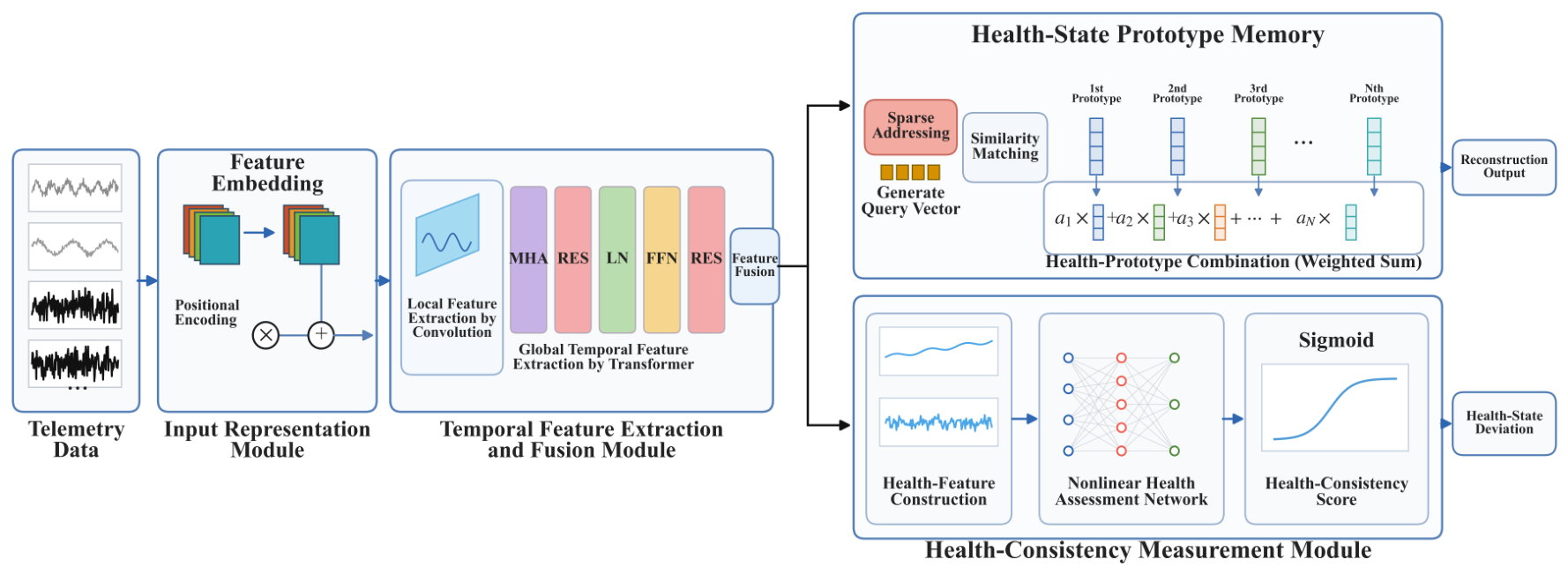
Figure 2.
Health-state prototype memory workflow.
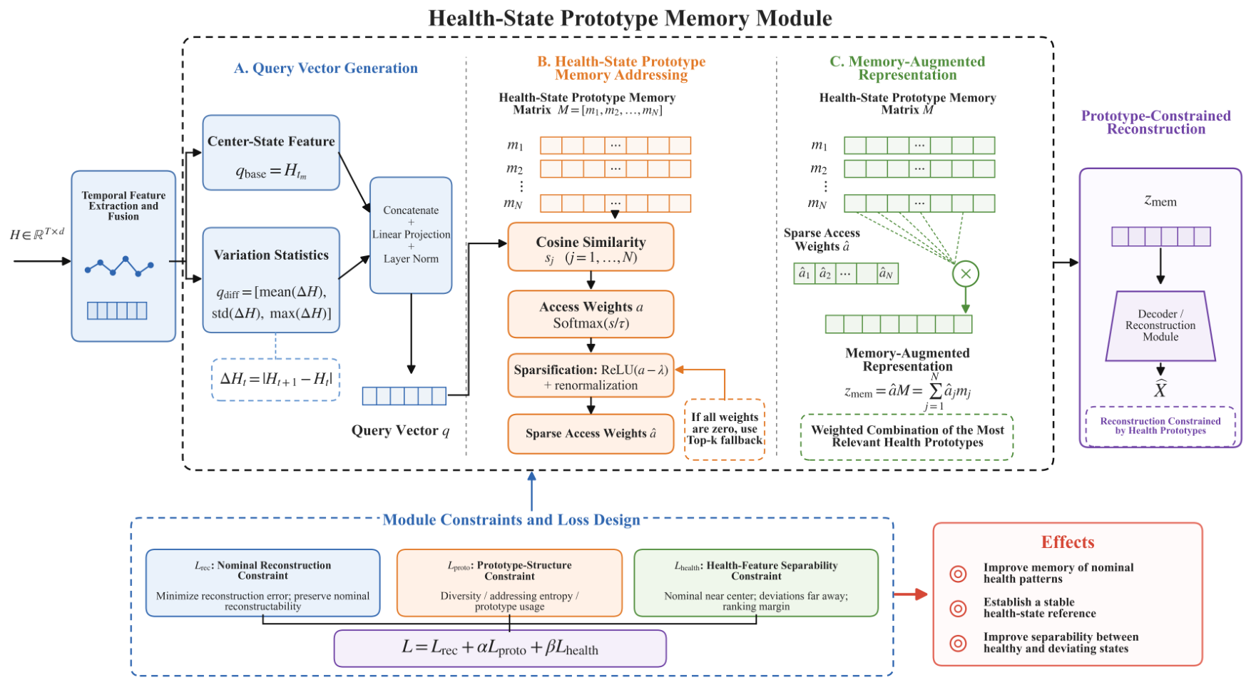
Figure 3.
Evaluation results of state deviation for different models: (a) first representative test sequence; (b) second representative test sequence.
Figure 3.
Evaluation results of state deviation for different models: (a) first representative test sequence; (b) second representative test sequence.
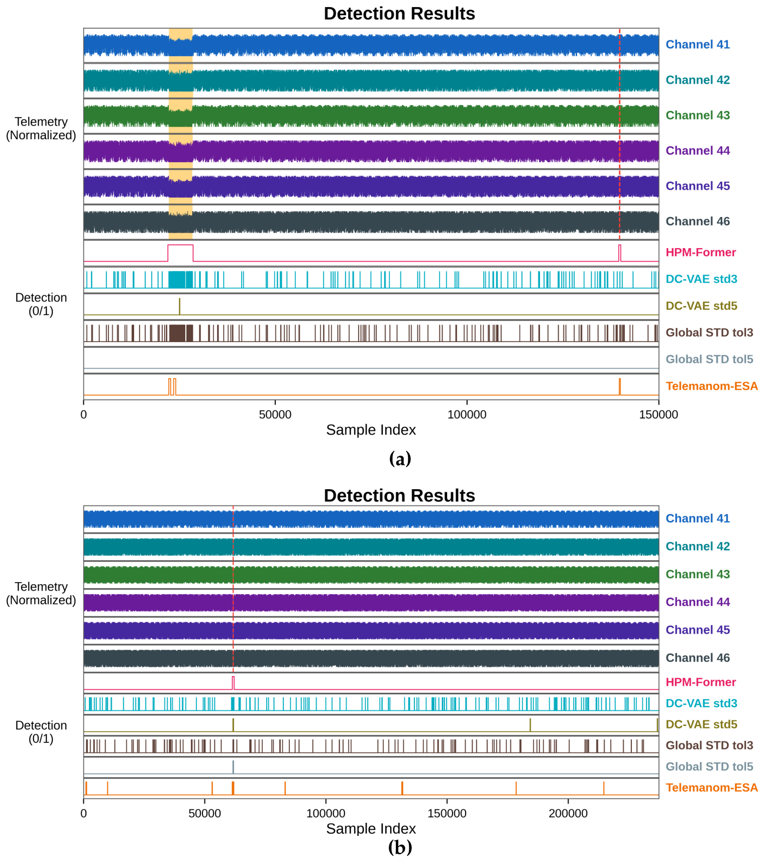
Figure 4.
Output comparison of the deep-learning models: (a) reconstruction output of DC-VAE; (b) prediction output of Telemanom.
Figure 4.
Output comparison of the deep-learning models: (a) reconstruction output of DC-VAE; (b) prediction output of Telemanom.
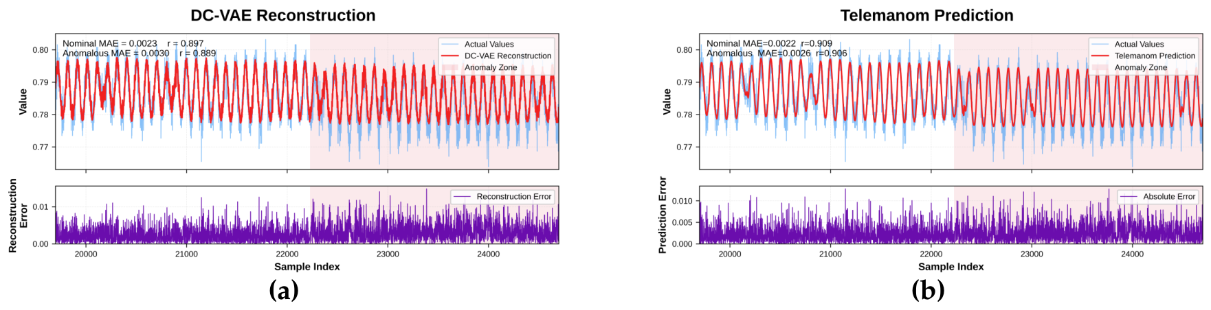
Figure 5.
Reconstruction comparison between Telemanom and HPM-Former.
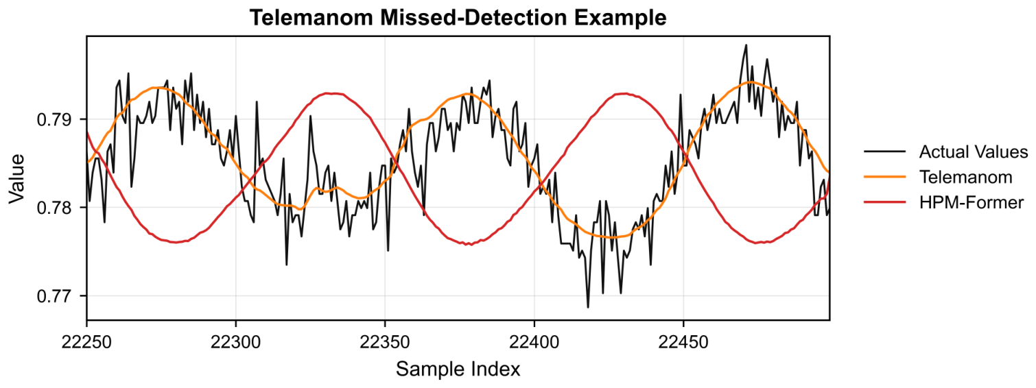
Figure 6.
Comparison of state-deviation decision distributions across different models: (a) joint anomaly-decision distribution of HPM-Former; (b) reconstruction-error distribution of DC-VAE.
Figure 6.
Comparison of state-deviation decision distributions across different models: (a) joint anomaly-decision distribution of HPM-Former; (b) reconstruction-error distribution of DC-VAE.
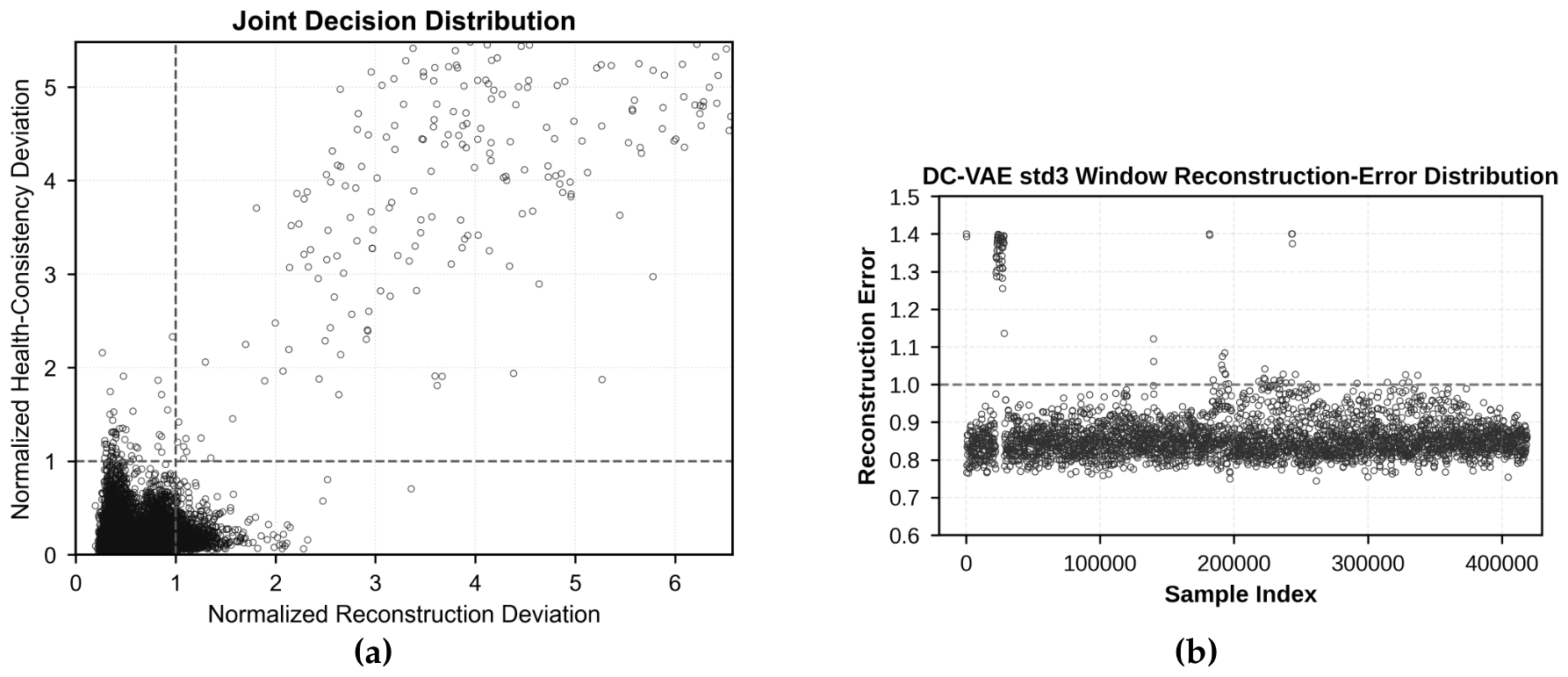

Table 1.
Main hyperparameter settings of HPM-Former.
| Parameter | Value | Parameter | Value |
|---|---|---|---|
| Latent dimension | 64 | Number of health-state prototypes | 128 |
| Number of attention heads | 4 | Dropout | 0.1 |
| Memory-addressing temperature | 0.12 | Sparse-access threshold | 0.01 |
| Top-k fallback size | 5 | Training batch size | 16 |
| Epochs | 50 | Optimizer | Adam |
| Learning rate | Test batch size | 128 | |
| State-separation loss weight | 0.5 | Health-consistency loss weight | 0.1 |
| Loss function | Mean squared error (MSE) | Convolution kernel size | 3 |
Table 2.
Experimental results.
| Method | ADTQC | ||||
|---|---|---|---|---|---|
| HPM-Former | 0.9967 | 1.0000 | 1.0000 | 0.2976 | 0.9237 |
| DC-VAE-STD3 | 0.0106 | 0.5667 | 0.0189 | 0.6667 | 0.6248 |
| DC-VAE-STD5 | 0.7692 | 0.3000 | 1.0000 | 0.9568 | 0.6046 |
| Telemanom | 0.4371 | 0.6923 | 0.8333 | 0.3993 | 0.7993 |
| Global-STD3 | 0.0123 | 0.5000 | 0.0231 | 0.6666 | 0.6809 |
| Global-STD5 | 0.5556 | 0.2000 | 1.0000 | 1.0000 | 0.4286 |
Table 3.
Ablation study results.
| Method | ADTQC | ||||
|---|---|---|---|---|---|
| HPM-Former | 0.9967 | 1.0000 | 1.0000 | 0.2976 | 0.9237 |
| Ablation model | 0.0010 | 0.7646 | 0.0083 | 0.7500 | 0.6949 |
Disclaimer/Publisher’s Note: The statements, opinions and data contained in all publications are solely those of the individual author(s) and contributor(s) and not of MDPI and/or the editor(s). MDPI and/or the editor(s) disclaim responsibility for any injury to people or property resulting from any ideas, methods, instructions or products referred to in the content. |
© 2026 by the authors. Licensee MDPI, Basel, Switzerland. This article is an open access article distributed under the terms and conditions of the Creative Commons Attribution (CC BY) license (http://creativecommons.org/licenses/by/4.0/).
Copyright: This open access article is published under a Creative Commons CC BY 4.0 license, which permit the free download, distribution, and reuse, provided that the author and preprint are cited in any reuse.