

Submitted:
03 September 2026
Posted:
07 September 2026
You are already at the latest version
Abstract
TikTok supports fashion discovery and creator-mediated brand communication. This study examines associations among TikTok fashion-brand content involvement, brand awareness, brand engagement, and purchase-related intentions among Bulgarian users and illustrates a human-governed analytical architecture for structured and open survey data. An online survey yielded 295 responses; 268 eligible TikTok users comprised the sample. The architecture organizes primary measurement and structural analysis, secondary prediction and moderation, exploratory segmentation and text analysis, and descriptive multi-criteria synthesis within processing stages. Content involvement was positively associated with awareness (β = 0.683), engagement (β = 0.512), and purchase-related intentions (β = 0.283). Awareness was associated with engagement (β = 0.300) but had no incremental direct association with purchase-related intentions; engagement showed the strongest direct association (β = 0.496). The model explained 52.5% of purchase-related-intention variance, and PLS-PM prediction produced lower errors than the training-mean benchmark for all four outcome indicators. No demographic interaction received Holm-adjusted support. Illustrative multi-criteria synthesis ranked engagement first, involvement second, and awareness third under sample-derived criteria. Dictionary-assisted open-response categories concerning presentation, creators, reviews, demonstrations, music, and humor were manually checked against the responses. Cross-sectional self-reports, concentrated sampling, broad working constructs, and internal validation require cautious, noncausal interpretation and independent external replication.
Keywords:
TikTok
; fashion-brand content
; brand awareness
; brand engagement
; purchase-related intentions
; intelligent survey-data analysis
; PLS path modeling
; business intelligence
; machine learning
; multi-criteria decision making
1. Introduction
Social media influencers have become important intermediaries between brands and consumers. They combine personal communication, content creation, product demonstration, and audience interaction, thereby shaping how sponsored and organic brand messages are encountered during the consumer decision process [1,2]. TikTok intensifies this role through short, rapidly changing videos in which entertainment, product information, creator identity, comments, sharing, and shopping cues appear in the same interface.
Fashion is particularly suitable for this environment because apparel and accessories are visually inspectable, identity-related, and responsive to trends. TikTok research shows that humor and hedonic experience can support influencer marketing outcomes [3], while brand-influencer communication is associated with engagement and purchase likelihood [4]. Fashion-specific studies further connect content quality, parasocial interaction, influencer credibility, attractive selling content, and attitudes towards TikTok videos with purchase-related outcomes [5,6,7,8].
Influencers should nevertheless not be treated as a uniformly effective marketing input. Their persuasive role depends on identification, similarity, trust, expertise, content value, and the relationship between creator and product [9,10,11]. Moreover, awareness, engagement, and purchase-related intentions represent different parts of the consumer response. A short video may make a brand recognizable without generating sufficient involvement to affect continued purchase, loyalty, or recommendation. This distinction is especially relevant when users encounter fashion content incidentally in an algorithmically curated feed.
Existing studies provide substantial evidence on influencer credibility and purchase intention, but fewer examine brand awareness (BA), brand engagement (BE), and broader purchase-related intentions in one TikTok fashion model. The literature is also concentrated in Asian markets and frequently focuses on livestream shopping, named influencers, or specific brands. Evidence from Central and Eastern Europe remains comparatively limited, and open consumer comments are rarely used to interpret pathways estimated from structured survey items.
The present study addresses this gap using Bulgarian survey data [12]. It evaluates a theory-guided association model in which TikTok fashion-brand content involvement (TCI) is specified as an antecedent of brand awareness (BA), brand engagement (BE), and purchase-related intentions (PRI), while BA and BE are specified as distinct correlates of PRI. This ordering follows the conceptual logic developed in Section 3; the cross-sectional design cannot establish temporal direction, and reverse or reciprocal relationships remain plausible. The dataset also contains open questions on content elements that attract attention and examples associated with brand opinions or purchasing decisions.
In this article, intelligent survey-data analysis denotes a human-governed combination of statistical modeling, machine learning, computer-assisted text processing, and rule-based quality control rather than autonomous artificial intelligence. The proposed architecture is illustrated through this case study; its transferability and comparative efficiency are not empirically validated here.
The study addresses four substantive research questions:
RQ1: How is involvement with TikTok fashion-brand content associated with brand awareness, brand engagement, and purchase-related intentions?
RQ2: Do brand awareness and brand engagement show distinct direct and statistical indirect associations between TikTok fashion-brand content involvement and purchase-related intentions under the specified model?
RQ3: Which content and creator categories are identified by dictionary-assisted coding and confirmed through manual review as attracting attention or being associated with fashion-brand responses?
RQ4: What response profiles emerge when purchase-related intentions are excluded from cluster formation, and how accurately can the antecedent indicators predict that outcome under repeated cross-validation?
A prespecified robustness check examines whether the construct-reliability conclusions remain stable after straight-line response profiles are excluded. This check is limited to reliability and does not re-estimate the structural model.
Illustrative analytical question (IAQ): How do TCI, BA, and BE rank when total structural association, incremental direct contribution, and internal predictive contribution are combined in a limited-scope MCDM synthesis?
Exploratory RQ5: Do gender, recorded age category, residence size, household income, or education show multiplicity-adjusted evidence of modifying any of the six specified associations?
The study makes two substantive contributions. It integrates TCI, BA, BE, and broad PRI in a compact association model and distinguishes the strong TCI–BA association from the more proximal BE–PRI association. It also examines whether demographic characteristics modify the six specified relationships, while treating their directions as theory-guided rather than causal.
Methodologically, the study proposes and illustrates a candidate human-governed analytical architecture. The measurement and PLS-PM association model is primary; prediction and demographic analysis are secondary; clustering and manually reviewed open-response coding are exploratory; and MCDM addresses a separate illustrative analytical question. This hierarchy prevents the methods from being treated as interchangeable evidence and keeps the questionnaire’s evidential boundary explicit: creator mentions are observed in open responses, but influencer credibility is not measured as a separate latent construct.
The remainder of the article reviews intelligent dataset-analysis frameworks (Section 2), presents the theoretical background and hypotheses (Section 3), introduces the proposed framework (Section 4), describes the study methods (Section 5), reports the results (Section 6), discusses their implications (Section 7), and concludes the article (Section 8).
2. Related Work on Intelligent Dataset-Analysis Frameworks
2.1. General Analytical Process Models
Intelligent dataset analysis is commonly organized as an iterative process rather than as a single algorithm. The knowledge-discovery-in-databases framework connects data selection, preprocessing, transformation, data mining, and interpretation [13]. CRISP-DM similarly links business understanding, data understanding, preparation, modeling, evaluation, and deployment [14]. CRISP-ML(Q) extends this logic for machine-learning systems by making quality assurance and monitoring explicit [15], while empirical software-engineering research shows that production machine learning also requires data discovery, feature engineering, testing, deployment, and monitoring activities that extend beyond model training [16]. These frameworks establish the need for iterative quality checks and traceable outputs, but they are not tailored to theory-based survey measurement.
2.2. Intelligent Analysis of Structured and Open Survey Data
Survey datasets combine response scales, construct definitions, demographic variables, and sometimes open text. Their analysis therefore requires more than generic preprocessing and prediction: measurement quality, common-source limitations, multiple testing, respondent heterogeneity, and the distinction between explanatory and predictive results must also be addressed. Clustering and machine learning can identify response patterns and internal predictive relationships, while natural-language processing can assist the coding of open answers. Research on automatic survey coding shows that model-assisted classification can reduce manual effort, but its validity depends on labeled data, coding design, and human verification [17]. Recent large-language-model annotation studies likewise indicate substantial potential for text coding while reinforcing the need for task-specific validation rather than assumed accuracy [18].
2.3. Research Gap
The reviewed approaches contribute important process, quality-assurance, engineering, and text-analytic elements, but none provides a survey-specific sequence connecting construct measurement, theory-guided structural analysis, exploratory segmentation, repeated prediction, open-text interpretation, and descriptive synthesis. Table 1 summarizes this gap. The candidate architecture assigns these roles to three nested processing levels and uses explicit pass/revise conditions under human review.
The comparison in Table 1 shows that the proposed architecture does not replace established process models; it combines their iterative and quality-assurance principles with requirements specific to theory-based survey research. Its role is to coordinate measurement assessment, explanatory modeling, exploratory segmentation, internal prediction, manually reviewed text analysis, and limited-scope multi-criteria synthesis while preserving the evidential limits of each method. This synthesis provides the methodological basis for the construct model in Section 3 and the governed analytical stages presented in Section 4.
3. Theoretical Background and Hypotheses
3.1. TikTok Fashion-Brand Content and Creator-Mediated Communication
Influencer communication combines source characteristics with message characteristics. Consumers may respond to a creator because the creator appears relatable or trustworthy, because the content is informative or entertaining, or because both mechanisms operate together [9,10,11]. In fashion, creators can reduce the distance between a product image and an imagined consumption experience by showing fit, styling, use situations, combinations, and personal evaluations. These demonstrations can also invite comments, imitation, and sharing.
The present questionnaire does not isolate creator credibility, attractiveness, expertise, or creator type. Its exogenous block measures interest in TikTok information about fashion brands, perceived information sufficiency, information sharing, and attention to fashion advertising. We refer to this block as TikTok fashion-brand content involvement (TCI). For this study, the common variance among the four indicators is interpreted as a general orientation to attend to, appraise, and use TikTok fashion-brand information. This rationale supports a reflective working specification, although the facets are not conceptually interchangeable; formative and multidimensional alternatives remain plausible.
3.2. Brand Awareness
Brand awareness concerns the accessibility of brand knowledge in memory, including recognition and recall [19]. Repeated exposure to distinctive visual, verbal, and sonic cues can make fashion brands easier to identify. On TikTok, creator demonstrations, recurring formats, hashtags, and participatory trends can reinforce these cues. Informative and credible influencer content has previously been connected with brand awareness [11]. Accordingly:
H1.
Involvement with TikTok fashion-brand content is positively associated with brand awareness.
3.3. Brand Engagement
Consumer brand engagement represents cognitive, affective, and behavioral investment in brand interactions [20]. In a short-video environment, engagement can include focused attention, positive affect, perceived connection with other users, and participation in brand-related activities. Entertaining, useful, and relatable creator content may be associated with these responses. Under the specified model, BA was hypothesized to be positively associated with BE.
H2.
Involvement with TikTok fashion-brand content is positively associated with brand engagement.
H4.
Brand awareness is positively associated with brand engagement.
3.4. Purchase-Related Intentions
Purchase intention is a stated willingness or likelihood to buy and is a proximal, imperfect indicator of subsequent behavior [21,22]. The present four-item block additionally includes continued purchase, loyalty, and recommendation. These items share a favorable future-oriented response to fashion brands encountered on TikTok, which motivates their use as a broad reflective working block named purchase-related intentions (PRI). However, they refer to different behavioral stages and may presuppose different levels of prior brand experience. PRI should therefore not be interpreted as a pure purchase-probability measure, a homogeneous single behavior, or observed sales.
H3.
Involvement with TikTok fashion-brand content is positively associated with purchase-related intentions.
H5.
Brand awareness is positively associated with purchase-related intentions.
H6.
Brand engagement is positively associated with purchase-related intentions.
The association model is informed by stimulus–organism–response (SOR) reasoning [23]. TCI is positioned first as a content-related appraisal, BA as cognitive accessibility, BE as relational investment, and PRI as the broad stated outcome. This ordering provides the theoretical rationale for the arrows, but the variables were measured at one time point. The arrows therefore denote theory-guided associations rather than observed temporal or causal effects; reverse, reciprocal, and contemporaneous alternatives remain plausible. Recent short-video studies similarly connect content appraisals with internal evaluations and purchase-related intentions [24,25]. Figure 1 summarizes the specified relationships.
3.5. Demographic Moderation as an Exploratory Research Question
Consumer responses to fashion-brand content may differ with digital familiarity, purchasing resources, education, and residential context. However, existing evidence does not establish consistent directional predictions for five demographic characteristics across all six model relationships. Demographic moderation is therefore examined as an exploratory research question rather than a single omnibus hypothesis.
RQ5: Do gender, recorded age category, residence size, household income, or education show multiplicity-adjusted evidence of modifying any of the six specified associations?
3.6. Comparison with Previous Empirical Models
Table 2 positions the model against selected empirical studies. Previous work commonly emphasizes credibility, trust, attitude, entertainment, or parasocial interaction. The present study complements these approaches by testing whether awareness and engagement have distinct roles in a TikTok fashion context, describing outcome-excluded response profiles, evaluating internal prediction, and using manually reviewed open responses to identify concrete content and creator categories.
Table 2 indicates that previous studies support links between content appraisals, awareness, engagement-related mechanisms, and purchase intentions, but generally examine only subsets of the relationships combined here. The present model specifies TCI as an antecedent construct, BA and BE as distinct consumer responses, and PRI as a broad outcome, while demographic moderation is examined separately. These directions define the explanatory component of the analytical architecture introduced in Section 4; they do not establish temporal ordering and do not exclude reverse or reciprocal models.
4. Proposed Human-Governed Framework for Intelligent Survey-Data Analysis
4.1. Framework Logic
The proposed candidate architecture adapts the iterative logic of KDD, CRISP-DM, and CRISP-ML(Q) to theory-based survey research [13,14,15]. Intelligent analysis denotes a governed combination of statistical modeling, data mining, machine learning, computer-assisted text processing, and rule-based quality control rather than autonomous artificial intelligence. The architecture is demonstrated here as a case-specific workflow, not as an empirically validated universal model.
Figure 2 organizes the architecture into three nested levels. Level 1 defines the analysis cycle; Level 2 specifies governed processing, quality gates, corrective feedback, and human interpretation; and Level 3 integrates measurement assessment, complementary analytical branches, diagnostic review, and illustrative synthesis. Human decisions remain necessary when defining constructs, checking eligibility, validating text categories, selecting synthesis criteria and weights, and interpreting results.
An additional advantage is software independence. The analytical stages can be implemented using paid commercial platforms or free and open-source environments, allowing researchers and organizations to select tools according to expertise, data-governance requirements, interoperability, infrastructure, and budget. In this study, the principal workflow was executed in R 4.4.1 using RStudio 2024.04.2, illustrating a reproducible implementation without mandatory software-license costs. Because the architecture defines analytical roles, quality gates, feedback loops, and outputs rather than vendor-specific commands, the same governed sequence can be implemented in other software ecosystems.
4.2. Analytical Stages
At Level 1, the analysis begins with the research objective and explicitly delimited decision question. Level 2 governs the ingestion of structured items, open responses, and metadata. Its first gate checks the input schema, codebook agreement, eligibility rule, missingness, valid 1–5 integer responses, duplicate and near-duplicate flags, response quality, translation, and categorical coding. A failed check leads to correction, exclusion under a stated rule, or documented limitation before analysis proceeds.
Level 3 begins with measurement assessment. It estimates construct scores and evaluates loadings, alpha, omega, composite reliability, AVE, and HTMT. These diagnostics are admissibility checks rather than proof of conceptual unidimensionality; uninterpretable measures require revision before downstream analysis, and AVE is not used as a marketing-relevance criterion.
To control analytical scope, the architecture assigns distinct evidential roles. Measurement assessment and the PLS-PM structural association model are primary; repeated internal prediction and demographic analyses are secondary; response-quality auditing, clustering, heatmaps, and manually verified open-response coding are exploratory; and MCDM is an illustrative descriptive synthesis. These roles answer different questions and do not validate one another independently.
The second gate evaluates measurement and reliability sensitivity, bootstrap-supported structural conclusions, demographic robustness, internal prediction benchmarks, cluster-validation indices, multiplicity-controlled tests, and completion of the manual text-verification procedure. Failed checks return the workflow to data processing, specification, or analysis revision. Outputs that pass may enter the limited-scope synthesis of total association with PRI, direct f2 on PRI, and grouped predictive importance.
Level 1 defines the overall analysis cycle. Level 2 specifies ingestion, operational quality checks, corrective feedback, and human interpretation. Level 3 integrates measurement assessment, complementary analytical branches, diagnostic review, and illustrative synthesis. Dictionary-assisted open-response assignments were manually verified before descriptive reporting.
5. Materials and Methods
5.1. Data Collection and Analytical Sample
The source file contained 295 anonymous online questionnaire responses recorded in Bulgaria between 30 November 2025 and 7 May 2026. Participation was restricted to respondents aged 18 years or older. The questionnaire was administered in Bulgarian. Structured variables and response categories were translated into English, while the original values were retained in the analysis workbook. For the open questions, one member of the research team manually checked all English translations and category assignments against the original Bulgarian responses; ambiguous cases were discussed within the research team. Because the available file contains neither a complete sampling frame nor an invitation log, the data are treated as a nonprobability, self-selected sample, and a conventional response rate cannot be reconstructed.
The principal analysis includes respondents who reported using TikTok and having encountered fashion-brand content. This deterministic eligibility rule retained 268 cases and excluded 27 records before model estimation. The excluded responses were not reintroduced as a robustness sample because they fall outside the population defined for the analysis. All sixteen Likert indicators were complete in the principal sample. The de-identified source dataset is publicly available in Mendeley Data [12].
5.2. Measurement Instrument
The model contains four reflectively specified working constructs measured on a five-point Likert scale (1 = strongly disagree; 5 = strongly agree). BA items follow recognition and recall logic [19], and BE items represent attention, affect, connection, and participation [20]. PRI combines planned purchase, continued purchase, loyalty, and recommendation as a broad favorable behavioral-intention block [21]; these outcomes are related but not conceptually identical. TCI represents a proposed orientation to attend to, appraise, and use TikTok fashion-brand information through interest, information sufficiency, sharing, and advertising attention. Treating TCI and PRI as reflective and approximately continuous is an empirical working specification, not proof of unidimensional conceptual identity. Full item wording is reported in Table 3.
5.3. Quantitative Analysis
The quantitative results were produced in R 4.4.1 using RStudio 2024.04.2 under Windows 10. The principal packages were plspm 0.6.0, psych 2.6.5, pwr 1.3-0, cluster 2.1.6, mclust 6.1.1, ranger 0.18.0, e1071 1.7-16, and gbm 2.2.3.
PLS-PM was selected for the primary prediction-oriented association model; it was not selected to establish causality. Among the complementary analyses, standardized PLS-PM construct scores were used in the two-stage demographic moderation models. The remaining complementary analyses used purpose-specific inputs: clustering used standardized equal-weight TCI, BA, and BE means; machine learning used the 12 TCI, BA, and BE indicators to predict the equal-weight PRI mean; and MCDM combined total structural association with PRI, direct f2 on PRI, and grouped predictive ΔRMSE. Reflective measurement assessment used loadings, Cronbach’s alpha, approximate omega total, composite reliability, AVE, and HTMT [26,27,28]. Structural assessment used standardized path coefficients, bootstrap intervals, R2, structural VIF, f2, and statistical indirect associations [29]. The model used path weighting, reflective Mode A blocks, and scaled data. No competing structural specification was estimated; parallel-predictor and alternative BA–BE orderings remain for future sensitivity analysis.
Main-path and indirect-effect uncertainty was estimated from 10,000 case-resampling bootstrap samples using sample.int(); stats::sd() and stats::quantile() supplied bootstrap standard errors and percentile intervals. HTMT was evaluated against the prespecified 0.85 descriptive threshold; no bootstrapped HTMT inference was performed. With n = 268 and a maximum of three predictors in an endogenous equation, pwr::pwr.f2.test() indicated a minimum detectable f2 of 0.041 at α = 0.05 and power = 0.80 for the main-effect regression setting. This sensitivity calculation does not establish adequate power for small demographic interactions or sparse subgroup contrasts.
Out-of-sample prediction was examined through repeated 10-fold cross-validation with 10 repetitions. The script’s run_pls_predict() routine re-estimated the PLS model, scaling, structural regressions, and indicator prediction equations within every training fold. Fold-specific regressions and predictions used stats::lm() and stats::predict(). Q2predict was calculated against the training-mean benchmark, and RMSE and MAE were also compared with a linear-regression benchmark [30]. The full-collinearity diagnostic was derived from auxiliary stats::lm() regressions; values below 3.3 do not eliminate same-source bias in a cross-sectional survey [31,32]. The 27 ineligible records were retained in the raw-data sheet but were not used as a sensitivity model.
To assess whether use intensity or fashion-content exposure distinguished the observed outcomes, Kruskal-Wallis tests compared equal-weight BA, BE, and PRI means across the original categories. The tests were obtained with stats::kruskal.test(), and stats::p.adjust(method = “holm”) controlled family-wise error across the six tests [33]. These comparisons are descriptive and do not identify causal exposure effects.
Demographic moderation was evaluated exploratorily using two-stage interaction models based on standardized PLS-PM construct scores [26,27]. Five binary moderators were used to avoid sparse categories: women versus men; the youngest recorded age category (‘Under 20’) versus the two older recorded categories (21–30 and 31 or older); residence in settlements with 50,000 residents or fewer versus larger settlements; household income below versus above BGN 1547 (approximately EUR 791) per household member; and secondary versus higher education. All participants were at least 18 years old. However, the supplied age categories do not separately identify respondents aged 18, 19, or 20; consequently, the moderation contrast is interpreted as a recorded age-category comparison rather than a precise age threshold. Each structural equation included its original predictors, the moderator main effect, and all corresponding interactions. Holm correction controlled the 30 path-specific tests. RQ5 was addressed by asking whether any interaction received adjusted support; omnibus block tests were treated as secondary diagnostics.
As a complementary robustness analysis, the five demographic variables were also entered simultaneously as direct covariates in the BA, BE, and PRI equations. The companion fit_demographic_effect_equation() routine used stats::lm.fit() for the original and adjusted equations and stats::pf() for the nested demographic-block comparisons. Case-resampling bootstrap intervals were calculated for each adjusted demographic direct effect and for changes in the six original structural coefficients. Holm correction through stats::p.adjust() was applied separately to the three demographic-block tests, the 15 direct-effect tests, the six adjusted structural paths, and the six coefficient-change tests. This analysis assesses robustness to demographic adjustment and is distinct from the interaction-based moderation analysis.
5.4. Exploratory Data Quality, Segmentation, and Machine-Learning Analysis
An additional data-quality audit examined duplicate response identifiers and timestamps, exact and near-duplicate structured profiles, missingness, response-range and integer consistency, eligibility-flag agreement, straight-line responding, and low within-person variation. Exact structured profiles were flagged with duplicated(), while near-duplicate item profiles within the same response context were screened using stats::dist(method = “manhattan”). Row-wise stats::sd() and run-length encoding through rle() supported the straight-line and long-string checks. Flagged profiles were documented rather than automatically deleted because anonymous response similarity does not establish respondent identity. Reliability diagnostics included standardized alpha, approximate omega total, corrected item-total correlations, alpha if an item was deleted, and item-level floor and ceiling percentages. As a prespecified robustness check, the 25 straight-line profiles were excluded and construct reliability was re-estimated [34,35]. The structural, clustering, predictive, and MCDM analyses were not re-estimated after this exclusion; therefore, the check supports only the stability of the reported reliability conclusions.
Exploratory response structure was first visualized from the 16 standardized indicators using pairwise Euclidean respondent dissimilarities and Ward.D2 hierarchical heatmaps. Standardization used scale(); Euclidean distances, Ward trees, and heatmaps used stats::dist(), stats::hclust(method = “ward.D2”), and stats::heatmap(), respectively. One heatmap clustered respondents and a second clustered indicators; respondent labels were suppressed because records were anonymous and the dendrograms were used descriptively. Exploratory segmentation then used standardized equal-weight means for TCI, BA, and BE; PRI was excluded from cluster formation. K-means solutions for k = 2–6 were estimated with stats::kmeans(nstart = 100, iter.max = 1000) and assessed using cluster::silhouette(), a directly calculated Calinski–Harabasz index, and the custom davies_bouldin_index() function [36,37,38]. The solutions for k = 2–5 were projected onto the first two principal components using stats::prcomp(), while cluster selection remained based on the full standardized equal-weight TCI, BA, and BE mean-score space. Ward hierarchical clustering and mclust::adjustedRandIndex() provided an algorithmic stability comparison [39]. Cluster means were interpreted as provisional response profiles, not population segments or causal types.
A separate internal prediction analysis estimated the equal-weight PRI mean from the 12 TCI, BA, and BE indicators using 10-fold cross-validation repeated five times. The target was an equal-weight PRI score, not the PLS-PM construct score, so the predictive and structural outcomes are closely related but not identical. Linear regression, ridge regression, radial-basis support-vector regression, random forest [40], extra trees, and gradient boosting were compared with the training-mean benchmark. Hyperparameters were fixed before performance evaluation as transparent, nonoptimized specifications; no outcome-based search was conducted. Performance was summarized across 50 held-out folds. Grouped permutation importance was descriptive, and no formal uncertainty test compared the ensemble models. Outcome indicators were never included among their own predictors.
5.5. Open-Response Analysis
The two open questions asked which TikTok content elements attract attention to a fashion brand (column Z) and requested an example associated with a brand opinion or purchase decision (column AA). The English translations were analyzed after applying the principal-sample eligibility rule. An R 4.4.1 script normalized the text and produced multi-label dictionary assignments, candidate counts, and token frequencies. The coding dictionary and category set were fixed before manual verification, and no new categories were introduced during that stage. One member of the research team manually reviewed all row-level English translations and dictionary-assisted assignments against the original Bulgarian responses. Ambiguous cases were discussed within the research team, after which the final assignments and reported counts were confirmed. Punctuation-only entries were retained in the nonempty denominators and coded as no relevant answer. Percentages use the number of nonempty responses to each question and may exceed 100% because labels are nonexclusive. This was deductive category verification rather than independent inductive thematic analysis [41]. Because the records were not independently double-coded, no intercoder-agreement statistic was calculated. The text categories were not used in structural estimation, prediction, clustering, or MCDM.
5.6. Illustrative Multi-Criteria Synthesis
MCDM addressed the illustrative analytical question after the measurement, structural, and predictive analyses. The limited-scope comparison considered TCI, BA, and BE under three sample-derived benefit criteria: total structural association with PRI, direct f2 on PRI, and grouped predictive ΔRMSE. Measurement quality was an admissibility condition and was not weighted; the alternatives were measured constructs rather than campaigns or interventions.
6. Results
6.1. Respondent Profile and Construct Descriptives
The principal sample consisted predominantly of women (76.9%) and respondents in the youngest recorded age category (‘Under 20’; 66.4%); a further 30.6% were recorded as aged 21–30. Daily TikTok use was reported by 87.7%, and 70.9% reported often encountering fashion-brand content. The profile therefore represents a young, highly active TikTok audience rather than the Bulgarian population as a whole.

Table 4.
Profile of the principal analysis sample (n = 268).
| Characteristic | Category | n | % |
| Gender | Female | 206 | 76.9 |
| Male | 62 | 23.1 | |
| Age | Under 20 | 178 | 66.4 |
| 21–30 | 82 | 30.6 | |
| 31 or older | 8 | 3.0 | |
| Residence | >50,000 residents | 139 | 51.9 |
| 1,000–50,000 | 115 | 42.9 | |
| <1,000 | 14 | 5.2 | |
| TikTok use | Daily | 235 | 87.7 |
| Weekly | 13 | 4.9 | |
| Rarely | 20 | 7.5 | |
| Fashion content | Often | 190 | 70.9 |
| Sometimes | 64 | 23.9 | |
| Very rarely | 14 | 5.2 |
The data-quality audit found no duplicate response identifiers or timestamps, no missing Likert responses, no out-of-range or noninteger Likert values, and no disagreement between the stored eligibility flag and the questionnaire rule. Three pairs of identical profiles across the predefined structured comparison variables were identified. Two pairs—records 4 and 50 and records 13 and 57 – were among the 268 eligible respondents, whereas one pair – records 264 and 281- was among the 27 excluded respondents. These are not completely duplicated records because timestamps, municipalities, and/or open responses differ. Twenty-five principal-sample records showed straight-line responding across all 16 audited indicators; they were retained in the primary analysis and examined through sensitivity checks rather than treated as automatically invalid.
In terms of geographic distribution, municipality names were normalized to correct spelling, capitalization, and administrative-prefix variants before calculating the distributions. Among the 268 eligible respondents, the largest share was from Plovdiv Municipality (125 respondents; 46.6%), followed by Asenovgrad (11 respondents; 4.1%). Burgas and Pazardzhik were each represented by nine respondents (3.4%). Overall, the eligible sample was strongly concentrated in the South Central Region (217 respondents; 81.0%), followed by the South East Region (40 respondents; 14.9%) and the South West Region (6 respondents; 2.2%). The remaining five respondents (1.9%) were distributed across the North West, North Central, and North East regions.
Brand awareness had the highest mean (M = 3.422), followed by TCI (M = 3.042) and brand engagement (M = 2.937). Purchase-related intentions were lower (M = 2.565), indicating that recognition and content involvement did not automatically translate into strong purchase-related responses. All construct correlations were positive, with the strongest associations between TCI and BE (r = 0.710) and between BE and PRI (r = 0.696).
Table 5.
Construct descriptives and correlations.
| Construct | Mean | SD | TCI | BA | BE | PRI |
| TCI | 3.042 | 0.974 | 1.000 | |||
| BA | 3.422 | 0.982 | 0.683 | 1.000 | ||
| BE | 2.937 | 0.989 | 0.710 | 0.647 | 1.000 | |
| PRI | 2.565 | 0.992 | 0.633 | 0.509 | 0.696 | 1.000 |
Respondent-level distances based on all 16 standardized indicators showed a broad, continuous response-intensity gradient (Figure 3). Blocks of relatively similar profiles were visible, but no sharp discontinuity justified treating the sample as naturally dichotomous. The matrix is a descriptive diagnostic and did not enter the PLS-PM estimation.
6.2. Reflective Measurement Assessment
All indicator loadings exceeded 0.70. Alpha and CR values exceeded 0.80, approximate omega ranged from 0.834 to 0.932, and AVE ranged from 0.665 to 0.831. The lowest corrected item-total correlation was 0.561 (TCI2), and item-deletion diagnostics did not provide a reliability-based reason to remove an indicator. The largest HTMT value was 0.822 (TCI–BE), below the prespecified 0.85 descriptive threshold; bootstrapped HTMT inference was not conducted. After excluding the 25 straight-line profiles, alpha remained acceptable for every construct (0.797–0.914). These diagnostics support the internal consistency of the four working reflective blocks in this sample, but they do not establish content validity or rule out formative or multidimensional TCI specifications and narrower PRI specifications.
Table 6.
Reflective measurement-model assessment.
| Construct | Items | Loading range | Alpha | Omega | CR | AVE |
| TCI | 4 | 0.730–0.871 | 0.832 | 0.834 | 0.888 | 0.665 |
| BA | 4 | 0.805–0.882 | 0.882 | 0.884 | 0.919 | 0.740 |
| BE | 4 | 0.851–0.890 | 0.890 | 0.890 | 0.924 | 0.751 |
| PRI | 4 | 0.897–0.927 | 0.932 | 0.932 | 0.952 | 0.831 |
Note: Omega denotes approximate omega total.
6.3. Structural Model and Hypothesis Tests
Five of the six hypothesized associations received bootstrap support. TCI was positively associated with BA (β = 0.683), BE (β = 0.512), and PRI (β = 0.283). BA was positively associated with BE (β = 0.300) but had no incremental direct association with PRI after TCI and BE were included (β = −0.002, p = 0.940). BE showed the strongest direct association with PRI (β = 0.496). The model explained 46.7% of BA variance, 56.2% of BE variance, and 52.5% of PRI variance. Structural VIFs ranged from 1.000 to 2.474. Effect sizes were large for TCI → BA (f2 = 0.876), moderate for TCI → BE (0.318) and BE → PRI (0.227), small for BA → BE (0.109) and TCI → PRI (0.068), and negligible for BA → PRI. These coefficients apply to the aggregate working specifications of TCI and broad PRI and should not be attributed to their individual facets.
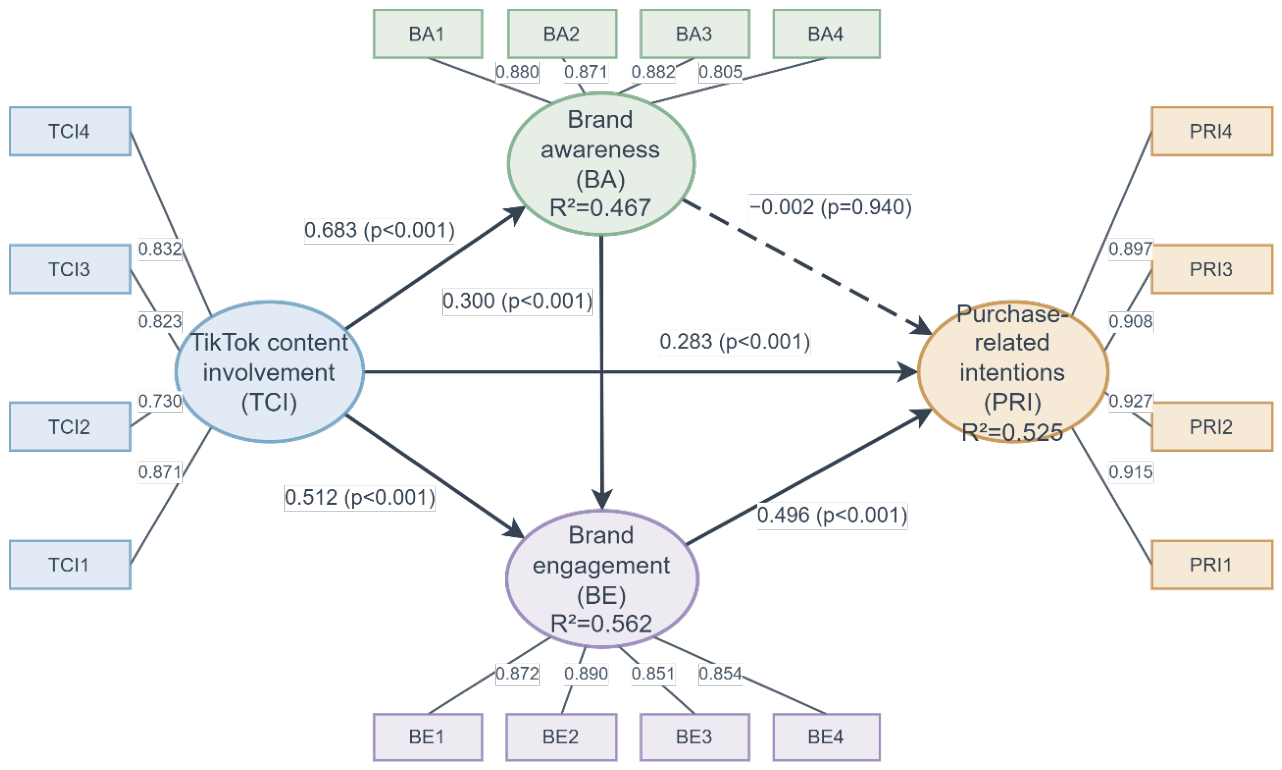
Table 7.
Structural paths and hypothesis results.
| Hypothesis | Relationship | β | SE | 95% CI | p | Decision | VIF | f2 |
| H1 | TCI → BA | 0.683 | 0.043 | [0.591, 0.760] | <0.001 | Supported | 1.000 | 0.876 |
| H2 | TCI → BE | 0.512 | 0.075 | [0.364, 0.655] | <0.001 | Supported | 1.876 | 0.318 |
| H3 | TCI → PRI | 0.283 | 0.077 | [0.135, 0.438] | <0.001 | Supported | 2.474 | 0.068 |
| H4 | BA → BE | 0.300 | 0.081 | [0.142, 0.462] | <0.001 | Supported | 1.876 | 0.109 |
| H5 | BA → PRI | −0.002 | 0.085 | [−0.168, 0.163] | 0.940 | Not supported | 2.082 | 0.000 |
| H6 | BE → PRI | 0.496 | 0.081 | [0.332, 0.651] | <0.001 | Supported | 2.282 | 0.227 |
Figure 4.
R 4.4.1-derived PLS-PM measurement and structural model. Values beside indicators are reflective loadings; values on paths are standardized coefficients with bootstrap p-values; values inside endogenous constructs are R2. The dashed BA → PRI path was nonsignificant.
Figure 4.
R 4.4.1-derived PLS-PM measurement and structural model. Values beside indicators are reflective loadings; values on paths are standardized coefficients with bootstrap p-values; values inside endogenous constructs are R2. The dashed BA → PRI path was nonsignificant.
6.4. Indirect Effects
The specified model yielded a nonsignificant TCI–BA–PRI statistical indirect association and positive TCI–BE–PRI and TCI–BA–BE–PRI indirect associations. Under this model, BA was associated with PRI statistically through BE (β = 0.149), while its incremental direct association with PRI was negligible. The total statistical indirect association from TCI to PRI was 0.354. These coefficient products describe model-dependent associations in cross-sectional data and do not establish temporal or causal mediation.
Table 8.
Bootstrapped indirect effects.
| Indirect relationship | β | SE | 95% CI | p |
| TCI → BA → PRI | −0.001 | 0.058 | [−0.118, 0.109] | 0.940 |
| TCI → BE → PRI | 0.254 | 0.051 | [0.160, 0.356] | <0.001 |
| TCI → BA → BE → PRI | 0.102 | 0.037 | [0.041, 0.185] | <0.001 |
| BA → BE → PRI | 0.149 | 0.052 | [0.062, 0.265] | <0.001 |
| TCI total indirect | 0.354 | 0.058 | [0.236, 0.465] | <0.001 |
6.5. Prediction and Group Comparisons
Repeated 10-fold cross-validation produced positive Q2predict values for all four PRI indicators. PLS RMSE and MAE values were lower than those of the training-mean benchmark in every case and were close to the linear-regression benchmark. The comparison therefore supports useful internal prediction without implying that PLS is uniformly superior to a simple linear model. The result has not been externally validated and should not be interpreted as a forecast of observed fashion purchases.
Table 9.
Repeated cross-validated prediction of purchase-related-intention indicators.
| Indicator | Q2predict | PLS RMSE | Linear RMSE | Mean RMSE | PLS MAE | Linear MAE | Mean MAE |
| PRI1 | 0.453 | 0.823 | 0.842 | 1.113 | 0.644 | 0.654 | 0.948 |
| PRI2 | 0.464 | 0.793 | 0.806 | 1.083 | 0.604 | 0.614 | 0.926 |
| PRI3 | 0.374 | 0.832 | 0.836 | 1.051 | 0.617 | 0.625 | 0.899 |
| PRI4 | 0.390 | 0.874 | 0.882 | 1.119 | 0.678 | 0.683 | 0.965 |
Full-collinearity VIFs ranged from 2.082 to 2.799, below 3.3. This auxiliary result reduces concern about severe common-method inflation but does not eliminate same-source or self-report bias. The 27 records failing the TikTok-use/content-exposure eligibility rule were not included in structural sensitivity analysis.
TikTok-use frequency did not distinguish BA, BE, or PRI after Holm correction. In contrast, self-reported fashion-content exposure distinguished all three outcomes: BA, H(2) = 20.807, pHolm < 0.001; BE, H(2) = 9.976, pHolm = 0.027; and PRI, H(2) = 23.948, pHolm < 0.001. Effect sizes were small to moderate (ε2 = 0.030–0.083). Respondents reporting frequent exposure had higher mean BA, BE, and PRI than those reporting very rare exposure. These unadjusted group differences may reflect self-selection or pre-existing interest and do not identify exposure effects.
Table 10.
Kruskal–Wallis comparisons across TikTok-use and fashion-content-exposure categories.
| Grouping variable | Outcome | H | df | p | pHolm | ε2 |
| TikTok use frequency | BA | 4.092 | 2 | 0.129 | 0.259 | 0.008 |
| TikTok use frequency | BE | 1.168 | 2 | 0.558 | 0.558 | 0.000 |
| TikTok use frequency | PRI | 5.495 | 2 | 0.064 | 0.192 | 0.013 |
| Fashion-content exposure | BA | 20.807 | 2 | <0.001 | <0.001 | 0.071 |
| Fashion-content exposure | BE | 9.976 | 2 | 0.007 | 0.027 | 0.030 |
| Fashion-content exposure | PRI | 23.948 | 2 | <0.001 | <0.001 | 0.083 |
6.6. Demographic Moderation
No path-specific demographic interaction received Holm-adjusted support; the smallest corrected value was pHolm = 0.948. The only nominal result was a gender interaction for BA → PRI (Δβ = −0.309, bootstrap p = 0.032, 95% CI [−0.615, −0.033]), but it did not survive correction. Its omnibus PRI interaction block added ΔR2 = 0.016 (F(3,260) = 3.081, raw p = 0.028, pHolm = 0.420). RQ5 therefore received no multiplicity-adjusted support in this sample; small moderation effects may remain undetected. The nominal result is reported for transparency and is not treated as a reproducible subgroup difference.
In the complementary demographic-adjustment models, adding gender, age, residence size, household income, and education increased R2 from 0.467 to 0.481 for BA, from 0.562 to 0.576 for BE, and from 0.525 to 0.540 for PRI (ΔR2 = 0.014, 0.015, and 0.015, respectively). None of the three demographic blocks was significant after Holm correction (all pHolm = 0.345). None of the 15 adjusted demographic direct effects survived correction; the smallest corrected value was pHolm = 0.216 for the gender coefficient in the BE equation. All five supported structural paths remained significant after adjustment, BA → PRI remained nonsignificant, and none of the six coefficient changes survived Holm correction. The original structural conclusions were therefore stable to simultaneous demographic adjustment.
Table 11.
Omnibus demographic interaction-block tests across the endogenous constructs.
| Moderator | Outcome | ΔR2 | F (df1, df2) | p | pHolm | Significant |
| Gender | BA | 0.002 | 0.758 (1, 264) | 0.385 | 1.000 | No |
| Gender | BE | 0.000 | 0.053 (2, 262) | 0.948 | 1.000 | No |
| Gender | PRI | 0.016 | 3.081 (3, 260) | 0.028 | 0.420 | No |
| Age | BA | 0.009 | 4.370 (1, 264) | 0.038 | 0.525 | No |
| Age | BE | 0.002 | 0.591 (2, 262) | 0.555 | 1.000 | No |
| Age | PRI | 0.009 | 1.689 (3, 260) | 0.170 | 1.000 | No |
| Residence size | BA | 0.008 | 4.004 (1, 264) | 0.046 | 0.603 | No |
| Residence size | BE | 0.006 | 1.894 (2, 262) | 0.153 | 1.000 | No |
| Residence size | PRI | 0.003 | 0.526 (3, 260) | 0.665 | 1.000 | No |
| Household income | BA | 0.005 | 2.568 (1, 264) | 0.110 | 1.000 | No |
| Household income | BE | 0.001 | 0.151 (2, 262) | 0.860 | 1.000 | No |
| Household income | PRI | 0.005 | 0.849 (3, 260) | 0.468 | 1.000 | No |
| Education | BA | 0.001 | 0.389 (1, 264) | 0.533 | 1.000 | No |
| Education | BE | 0.003 | 0.772 (2, 262) | 0.463 | 1.000 | No |
| Education | PRI | 0.000 | 0.071 (3, 260) | 0.975 | 1.000 | No |
Note: Omnibus p-values were Holm-adjusted across 15 interaction-block tests. RQ5 was evaluated primarily through 30 bootstrapped path-specific interactions; none received adjusted support.
6.7. Exploratory Segmentation and Machine-Learning Prediction
Across k = 2–6, k = 2 had the strongest internal validation profile: the highest silhouette coefficient (0.449) and Calinski–Harabasz index (278.755), and the lowest Davies–Bouldin index (0.865; Table 12). Ward and k-means agreement was substantial but not near-perfect (adjusted Rand index = 0.769). The solution separated 87 lower-rating and 181 higher-rating profiles. Because TCI, BA, and BE were strongly positively correlated, this division primarily reflects general response intensity rather than distinct consumer types. PRI was excluded from cluster formation; its post-cluster difference is descriptive and is expected to some extent from its correlations with the clustering variables. Temporal stability and external cluster validity were not assessed.
Table 12.
Internal validation of outcome-excluded k-means solutions.
| k | Total within-cluster SS | Silhouette | Calinski–Harabasz | Davies–Bouldin | Selected |
| 2 | 391.123 | 0.449 | 278.755 | 0.865 | Yes |
| 3 | 275.159 | 0.356 | 253.213 | 0.956 | No |
| 4 | 224.581 | 0.311 | 225.864 | 1.069 | No |
| 5 | 196.209 | 0.289 | 202.666 | 1.136 | No |
| 6 | 171.927 | 0.284 | 191.730 | 1.135 | No |
Note: Clusters were estimated from standardized equal-weight TCI, BA, and BE scores; PRI was excluded. Higher silhouette and Calinski–Harabasz values and lower Davies–Bouldin values indicate stronger separation. The within-cluster sum of squares decreases mechanically as k increases and was not used alone for selection.
The hierarchical views give a complementary item-level description. The respondent heatmap (Figure 5) shows broad lower- and higher-response bands while preserving substantial within-band variation. The indicator heatmap (Figure 6) recovers coherent within-construct groupings and also visualizes the comparatively close TCI–BE and BE–PRI relationships found in the correlation and structural analyses. These dendrograms summarize similarity; they do not establish a fixed number of latent classes.
The principal-component projections in Figure 7 make the selection trade-off visible. The k = 2 panel provides the clearest broad separation; solutions with three to five clusters subdivide the same response continuum and show increasing overlap in the two-dimensional projection. Because the panels display only the first two components, the formal selection is based on the full-space indices in Table 12 rather than on visual separation alone.
Table 13.
Outcome-excluded exploratory cluster profiles.
| Cluster | n | TCI mean | BA mean | BE mean | PRI mean |
| 1: Higher ratings | 181 | 3.528 | 3.887 | 3.443 | 2.975 |
| 2: Lower ratings | 87 | 2.032 | 2.454 | 1.882 | 1.713 |
Note: PRI was not used to form the clusters and was compared only after cluster assignment.
Random forest achieved the lowest mean fold-level error (RMSE = 0.651, SD = 0.103; MAE = 0.481, SD = 0.078) and the highest mean held-out R2 (0.521, SD = 0.170), improving RMSE by 34.1% relative to the training-mean benchmark. Gradient boosting and extra trees produced closely similar results, and no formal uncertainty test compared the ensemble methods. Grouped permutation analysis identified BE as the largest predictor group, followed by TCI and BA. The target was the equal-weight PRI mean rather than the PLS-PM construct score. These results describe internal predictive performance and require external validation.
Table 14.
Repeated 10-fold cross-validated prediction of the purchase-related-intentions mean.
| Model | RMSE (SD) | MAE (SD) | R2 (SD) | RMSE improvement (%) |
| Training-mean benchmark | 0.987 (0.120) | 0.841 (0.113) | −0.053 (0.087) | 0.0 |
| Linear regression | 0.696 (0.110) | 0.533 (0.078) | 0.451 (0.196) | 29.6 |
| Ridge regression | 0.692 (0.110) | 0.531 (0.078) | 0.457 (0.192) | 29.9 |
| SVR-RBF | 0.774 (0.133) | 0.586 (0.098) | 0.305 (0.305) | 21.6 |
| Random forest | 0.651 (0.103) | 0.481 (0.078) | 0.521 (0.170) | 34.1 |
| Extra trees | 0.673 (0.112) | 0.493 (0.084) | 0.486 (0.193) | 31.9 |
| Gradient boosting | 0.671 (0.104) | 0.512 (0.078) | 0.493 (0.169) | 32.1 |
Note: Values are means and standard deviations across 50 held-out folds (five repetitions of 10-fold cross-validation). R2 was computed separately within each held-out fold and then summarized across folds.
6.8. Open-Response Findings
The attention question contained 230 nonempty eligible responses, including three punctuation-only entries. After manual verification of the dictionary-assisted assignments against the original Bulgarian responses, presentation and visual style was assigned to 84 responses (36.5%), reviews or product demonstrations to 62 (27.0%), influencers or creators to 61 (26.5%), and music, humor, or entertainment to 48 (20.9%). No relevant experience was assigned to 12 responses (5.2%), authenticity or credibility to 9 (3.9%), and trends or participation to 7 (3.0%); price, promotion, or availability was not assigned for this question. The categories are descriptive and nonexclusive and do not measure the relative effectiveness of the identified content elements.
The influence-case question contained 201 nonempty eligible responses, including six punctuation-only entries. Manual verification assigned no relevant experience or recall to 38 responses (18.9%), presentation and visual style to 35 (17.4%), reviews or product demonstrations to 32 (15.9%), influencers or creators to 22 (10.9%), authenticity or credibility to 6 (3.0%), price, promotion, or availability to 6 (3.0%), and music, humor, or entertainment to 2 (1.0%). In the separate consequence coding, no relevant case or influence was assigned to 38 responses (18.9%), positive opinion or increased interest to 22 (10.9%), completed purchase to 9 (4.5%), brand discovery or awareness to 8 (4.0%), purchase consideration or intention to 8 (4.0%), and negative opinion, avoidance, or return to 3 (1.5%). The categories are descriptive, nonexclusive, and do not claim exhaustive thematic coverage or causal effects.
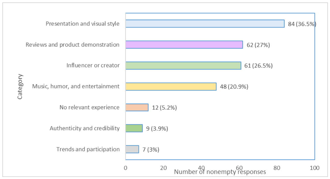
Figure 8.
Manually verified multi-label categories in responses concerning attention to TikTok fashion-brand content (n = 230 nonempty eligible responses). Dictionary-assisted assignments were checked against the original Bulgarian responses; the categories are descriptive and nonexclusive.
Figure 8.
Manually verified multi-label categories in responses concerning attention to TikTok fashion-brand content (n = 230 nonempty eligible responses). Dictionary-assisted assignments were checked against the original Bulgarian responses; the categories are descriptive and nonexclusive.
6.9. Illustrative Multi-Criteria Synthesis
Table 15 presents the fixed three-construct decision matrix. TCI had the largest total association with PRI, whereas BE had the largest direct f2 and grouped predictive contribution; BA had a negligible direct f2.
All four methods produced the same order under equal and CRITIC weights: BE first, TCI second, and BA third. This result indicates insensitivity to the examined aggregation formulas and weighting schemes for the fixed matrix.
7. Discussion
7.1. Interpretation of the Main Findings
The results distinguish awareness from broader purchase-related responses. TCI had its strongest association with BA, consistent with TikTok’s capacity to expose users repeatedly to distinctive fashion-brand cues. The manually verified open-response categories provide descriptive context: presentation and visual style was most frequent, while creators, demonstrations, music, and humor were also identified. These categories do not explain the structural association and should not be interpreted as comparative effectiveness evidence.
BE showed the strongest direct association with PRI, and the specified model yielded positive TCI–BE–PRI and BA–BE–PRI statistical indirect associations. Under this model, BA was associated with PRI indirectly through BE rather than through a separate direct association. This pattern is consistent with recognition being insufficient once attention, affect, connection, and participation are considered. Because PRI also includes continued purchase, loyalty, and recommendation, the interpretation concerns a broad purchase-related block rather than purchase intention alone.
The positive direct TCI–PRI association indicates that some TikTok content may be related to purchase-related intentions without passing entirely through the measured awareness and engagement blocks. Reviews, product demonstrations, links, promotions, or immediate creator recommendations may reduce search effort and support such responses. At the same time, the cross-sectional design does not show that changing these content features would cause a corresponding change in purchasing.
The exploratory analyses describe a broad response-intensity gradient rather than sharply isolated natural classes. The outcome-excluded two-cluster solution separated lower- and higher-rating profiles, but the correlated TCI, BA, and BE inputs mean that the solution largely reflects general response positivity. The post-cluster PRI difference is therefore descriptive and partly expected from PRI’s correlations with those inputs. The adjusted Rand index of 0.769 shows substantial, not near-perfect, agreement between k-means and Ward clustering. The profiles are not validated consumer types and their temporal stability is unknown.
The machine-learning results align descriptively with the structural model at the construct level: BE produced the largest grouped permutation contribution and was also the strongest direct structural correlate of PRI. Random forest had the lowest mean held-out error, but gradient boosting and extra trees were close and no formal uncertainty test established a difference between them. Moreover, machine learning predicted the equal-weight PRI mean, whereas PLS-PM used a model-derived construct score. The analyses are complementary rather than independent validation.
The illustrative synthesis ordered BE first, TCI second, and BA third across the examined formulas and weights. Because all criteria came from the same fixed sample-derived matrix, the order is a descriptive analytical summary rather than evidence about marketing interventions.
The moderation analysis provided no Holm-adjusted evidence that the specified associations differed by gender, recorded age category, residence size, household income, or education. The complementary adjustment models likewise showed no corrected demographic direct effect, significant demographic block, or Holm-adjusted change in any original structural coefficient. Thus, these analyses provide no multiplicity-adjusted evidence of demographic interaction or coefficient instability in this sample; they do not establish demographic invariance, and small effects may remain undetected. The nominal gender interaction requires independent replication.
7.2. Comparison with Previous Studies
The strong TCI–awareness association is consistent with Lou and Yuan [11], who connected trust in influencer-branded content with brand awareness and purchase intentions. The present model adds an important qualification: BA had no incremental direct association with PRI after BE and TCI were modeled simultaneously. This difference may arise because Lou and Yuan explicitly modeled trust in influencer posts, whereas the present TCI block measures content involvement and information behavior rather than creator credibility.
The central role of engagement is consistent with Hazari et al. [4] and complements studies emphasizing content quality, parasocial interaction, credibility, and relational mechanisms [5,6]. The manually verified open-response categories identified creators, presentation, reviews, and demonstrations. They provide descriptive context but do not isolate influencer effectiveness or support causal managerial claims.
The statistical indirect pattern also resembles the Vietnamese TikTok fashion-livestream study by Thuy and Quang [7], which linked streamer influence to purchase intention through attitude and trust. In the present specified model, the TCI–BA–BE–PRI coefficient product is consistent with an indirect association involving BA and BE. Because the data are cross-sectional, this comparison does not establish a temporal mechanism.
Music, humor, and entertainment were also identified in the manually reviewed categories. This descriptive pattern is compatible with Barta et al. [3], who emphasized humor and hedonic experience in TikTok influencer marketing, but it is not confirmatory evidence of effectiveness. The structured results also align with Lin et al. [8], who connected attitudes toward TikTok videos with sustainable-apparel purchase intention.
7.3. Theoretical and Methodological Implications
The study contributes to short-video and creator-mediated brand research by separating a cognitive brand outcome from a relational outcome. The association sequence is compatible with SOR reasoning, but TCI is a respondent appraisal rather than an experimentally controlled stimulus. Accordingly, the model shows that awareness and engagement do not have equivalent relationships with PRI without claiming a tested temporal stimulus–response mechanism.
The findings also clarify the level at which influencer claims can be made. The data support a role for TikTok fashion-brand content and creator cues, but not a comparison of influencer types or a causal effect of influencer credibility. Future models should add explicit measures of trustworthiness, expertise, similarity, parasocial interaction, sponsorship disclosure, and creator–brand fit to distinguish source effects from message effects.
Methodologically, the study illustrates a candidate human-governed architecture that separates primary PLS-PM analysis, secondary prediction and moderation, exploratory clustering and manually verified text coding, and descriptive synthesis. The roles are software-independent and can be implemented in commercial or free and open-source tools; R 4.4.1 and RStudio provide the present reproducible route. Transferability requires comparison with alternative workflows and testing in new samples and domains.
7.4. Managerial Implications
The findings suggest that fashion brands may benefit from evaluating TikTok activity beyond reach and recall indicators. Visual consistency and memorable presentation may accompany awareness, while sustained viewing, meaningful comments, saves, shares, creator–audience interaction, and product-related questions may be useful indicators of engagement associated with stronger purchase-related intentions.
The manually verified presentation, creator, review, demonstration, and entertainment categories can be treated as research-informed content hypotheses rather than proven tactics. Managerial use would require testing them against campaign exposure, clickstream, conversion, and sales data.
The lower- and higher-rating profiles may be used as provisional analytical descriptions when reviewing content responses, but they should not be converted directly into targeting rules. Before operational use, brands should verify profile stability in a new sample and determine whether the separation reflects substantive consumer differences, general response positivity, or prior interest in fashion content.
7.5. Limitations and Future Research
Several limitations apply. First, the nonprobability Bulgarian sample is concentrated among women, younger respondents, and the South Central Region. Recruitment-channel coverage and a conventional response rate cannot be reconstructed. Participation was restricted to adults. Nevertheless, the recorded category ‘Under 20’ does not distinguish respondents aged 18 from those aged 19 and does not explicitly represent age 20; the age composition and moderation results should therefore be interpreted as recorded category contrasts rather than precise age thresholds. Second, all key constructs were measured in one cross-sectional survey, so temporal order and causality cannot be established and common-method bias remains possible.
Third, TCI combines interest, information sufficiency, sharing, and advertising attention as a reflective working construct; formative or multidimensional alternatives remain plausible. Fourth, PRI combines planned purchase, continued purchase, loyalty, and recommendation across different behavioral stages and does not measure actual sales. Fifth, the exploratory demographic contrasts may lack power for small or nonlinear interactions. No competing structural specification was estimated; parallel-predictor, reverse BA–BE, and other contemporaneous orderings should be evaluated in independent longitudinal or experimental data.
Sixth, the illustrative MCDM analysis ranks only three constructs using overlapping criteria derived from the same sample and does not propagate sampling or criterion-selection uncertainty. Its order should therefore be treated as a descriptive summary until replicated with independent data and stakeholder-defined alternatives, criteria, and weights.
Seventh, one researcher manually verified all dictionary-assisted assignments against the original Bulgarian responses using a category set fixed in advance; ambiguous cases were discussed within the team. The procedure confirms the reported deductive categories and counts but is neither independent double coding nor inductive thematic analysis, and it does not claim exhaustive coverage of meanings.
Future work should use probability-based or stratified samples, record age precisely, and collect longitudinal or experimental data linked to observed exposure and transactions. Measurement research should compare reflective, formative, and multidimensional TCI specifications and separate purchase intention from loyalty and recommendation. Competing structural directions, cluster stability, pooled out-of-fold predictive metrics, and uncertainty in MCDM ranks should be examined in independent samples. Preregistered external validation would permit stronger conclusions.
8. Conclusions
This study examined TikTok fashion-brand content using 268 eligible Bulgarian respondents. Under the specified PLS-PM model, TCI was positively associated with BA, BE, and broad PRI. BA was associated with BE but had no incremental direct association with PRI, whereas BE was the strongest direct correlate of PRI. All four PRI indicators showed positive internal predictive performance relative to a training-mean benchmark.
No demographic interaction received Holm-adjusted support across the 30 path-specific tests. RQ5 therefore yielded no multiplicity-adjusted evidence of moderation in this sample, although small effects may remain undetected. The nominal gender interaction involving BA → PRI requires independent replication.
The exploratory two-cluster solution described lower- and higher-rating response-intensity partitions without using PRI to form them. Because the inputs were strongly correlated and external or temporal cluster stability was not tested, the partitions are not distinct consumer types. Random forest provided the lowest mean prediction error for the equal-weight PRI mean, but other ensemble methods were close.
The illustrative synthesis ranked BE first, TCI second, and BA third for the fixed sample-derived matrix; this order is descriptive and does not establish causal or managerial priority.
The structured results indicate that TikTok fashion communication cannot be reduced to visibility: PRI was more closely associated with BE than with BA’s incremental direct contribution. Dictionary-assisted categories concerning presentation, creators, reviews, demonstrations, music, and humor were manually checked against the responses and may inform subsequent research. They remain descriptive categories rather than evidence that these content elements cause consumer outcomes.
The study therefore offers two limited-scope contributions. Substantively, it documents model-dependent associations among content involvement, awareness, engagement, and broad purchase-related intentions in a young, active Bulgarian TikTok sample. Methodologically, it proposes and illustrates a candidate human-governed architecture that assigns primary, secondary, exploratory, textual, and descriptive-synthesis roles to reproducible analytical stages. The architecture can be implemented using paid software or free and open-source tools; R 4.4.1 and RStudio provide the present reproducible route. Transferability and comparative effectiveness require testing in new samples, domains, and workflows.
Author Contributions
Conceptualization, G.I., T.Y., M.R., D.A., S.K.-B., M.B., P.G. and A.D.; modeling, G.I., T.Y., M.R. and S.K.-B.; validation, G.I., T.Y., M.R. and M.B.; formal analysis, T.Y.; resources, G.I., T.Y., M.R. and S.K.-B.; writing—original draft preparation, G.I.; writing—review and editing, G.I., T.Y. and P.G.; visualization, T.Y. and S.K.-B.; supervision, G.I.; project administration, M.R. and A.D.; funding acquisition, G.I., T.Y. and S.K.-B. All authors have read and agreed to the published version of the manuscript.
Funding
This research is supported by the Project BG16RFPR002-1.014-0013-C01 “Digitalization of Economy in Big Data Environment– Second Stage” (DIGD2) financed by the “Research, Innovation and Digitalization for Smart Transformation” Program 2021–2027 and co-funded by the European Union.
Institutional Review Board Statement
Ethical review and approval were not required for this study, as it did not involve any sensitive or personally identifiable data. Participation was voluntary and anonymous. All procedures complied with the EU General Data Protection Regulation (GDPR) and applicable national legislation.
Informed Consent Statement
Participants were informed about the purpose of the study, its voluntary and anonymous nature, and the intended use of the collected data. Participation was restricted to adults aged 18 years or older, and proceeding with the questionnaire was treated as informed consent.
Data Availability Statement
The de-identified dataset analyzed in this study is openly available in Mendeley Data, Version 1, at https://data.mendeley.com/drafts/dv9zw7cs5x [12].
Conflicts of Interest
The authors declare no conflicts of interest.
References
- Vrontis, D.; Makrides, A.; Christofi, M.; Thrassou, A. Social media influencer marketing: A systematic review, integrative framework and future research agenda. Int. J. Consum. Stud. 2021, 45, 617–644. [Google Scholar] [CrossRef]
- Hudders, L.; De Jans, S.; De Veirman, M. The commercialization of social media stars: A literature review and conceptual framework on the strategic use of social media influencers. Int. J. Advert. 2021, 40, 327–375. [Google Scholar] [CrossRef]
- Barta, S.; Belanche, D.; Fernandez, A.; Flavian, M. Influencer marketing on TikTok: The effectiveness of humor and followers’ hedonic experience. J. Retail. Consum. Serv. 2023, 70, 103149. [Google Scholar] [CrossRef]
- Hazari, S.; Talpade, S.; Brown, C.O. Do brand influencers matter on TikTok? A social influence theory perspective. J. Mark. Theory Pract. 2024, 32, 271–289. [Google Scholar] [CrossRef]
- Gomes, M.A.; Marques, S.; Dias, A. The impact of digital influencers’ characteristics on purchase intention of fashion products. J. Glob. Fash. Mark. 2022, 13, 187–204. [Google Scholar] [CrossRef]
- Alcantara-Pilar, J.M.; Rodriguez-Lopez, M.E.; Kalinic, Z.; Liebana-Cabanillas, F. From likes to loyalty: Exploring the impact of influencer credibility on purchase intentions in TikTok. J. Retail. Consum. Serv. 2024, 78, 103709. [Google Scholar] [CrossRef]
- Thuy, D.C.; Quang, N.N. Influence of livestream selling on purchase intention fashion products on TikTok. SAGE Open 2025, 15, 21582440251375733. [Google Scholar] [CrossRef]
- Lin, C.A.; Wang, X.; Dam, L. TikTok videos and sustainable apparel behavior: Social consciousness, prior consumption and theory of planned behavior. Emerg. Media 2023, 1, 46–69. [Google Scholar] [CrossRef]
- Schouten, A.P.; Janssen, L.; Verspaget, M. Celebrity vs. influencer endorsements in advertising: The role of identification, credibility, and product-endorser fit. Int. J. Advert. 2020, 39, 258–281. [Google Scholar] [CrossRef]
- Ki, C.-W.C.; Kim, Y.-K. The mechanism by which social media influencers persuade consumers: The role of consumers’ desire to mimic. Psychol. Mark. 2019, 36, 905–922. [Google Scholar] [CrossRef]
- Lou, C.; Yuan, S. Influencer marketing: How message value and credibility affect consumer trust of branded content on social media. J. Interact. Advert. 2019, 19, 58–73. [Google Scholar] [CrossRef]
- Ilieva, G.; Yankova, T.; Ruseva, M.; Angelov, D.; Klisarova-Belcheva, S.; Bratkov, M.; Georgiev, P.; Dimitrov, A. TikTok Fashion Marketing and Consumer Brand Responses: A Survey Dataset. Mendeley Data 2026, V1. Available online: https://data.mendeley.com/drafts/dv9zw7cs5x.
- Fayyad, U.; Piatetsky-Shapiro, G.; Smyth, P. From data mining to knowledge discovery in databases. AI Mag. 1996, 17, 37–54. [Google Scholar] [CrossRef]
- Shearer, C. The CRISP-DM model: The new blueprint for data mining. J. Data Warehous. 2000, 5, 13–22. [Google Scholar]
- Studer, S.; Bui, T.B.; Drescher, C.; Hanuschkin, A.; Winkler, L.; Peters, S.; Müller, K.-R. Towards CRISP-ML(Q): A machine learning process model with quality assurance methodology. Mach. Learn. Knowl. Extr. 2021, 3, 392–413. [Google Scholar] [CrossRef]
- Amershi, S.; Begel, A.; Bird, C.; DeLine, R.; Gall, H.; Kamar, E.; Nagappan, N.; Nushi, B.; Zimmermann, T. Software engineering for machine learning: A case study. In Proceedings of the 41st International Conference on Software Engineering: Software Engineering in Practice, Montreal, QC, Canada, 25–31 May 2019; pp. 291–300. [Google Scholar] [CrossRef]
- He, Z.; Schönlau, M. Automatic coding of open-ended questions into multiple classes: Whether and how to use double coded data. Surv. Res. Methods 2020, 14, 267–287. [Google Scholar] [CrossRef]
- Gilardi, F.; Alizadeh, M.; Kubli, M. ChatGPT outperforms crowd workers for text-annotation tasks. Proc. Natl. Acad. Sci. USA 2023, 120, e2305016120. [Google Scholar] [CrossRef] [PubMed]
- Keller, K.L. Conceptualizing, measuring, and managing customer-based brand equity. J. Mark. 1993, 57, 1–22. [Google Scholar] [CrossRef]
- Hollebeek, L.D.; Glynn, M.S.; Brodie, R.J. Consumer brand engagement in social media: Conceptualization, scale development and validation. J. Interact. Mark. 2014, 28, 149–165. [Google Scholar] [CrossRef]
- Spears, N.; Singh, S.N. Measuring attitude toward the brand and purchase intentions. J. Curr. Issues Res. Advert. 2004, 26, 53–66. [Google Scholar] [CrossRef]
- Morwitz, V.G. Consumers’ purchase intentions and their behavior. Found. Trends Mark. 2014, 7, 181–230. [Google Scholar] [CrossRef]
- Mehrabian, A.; Russell, J.A. An Approach to Environmental Psychology; MIT Press: Cambridge, MA, USA, 1974. [Google Scholar]
- Luo, C.; Mohd Hasan, N.A.; Zamri bin Ahmad, A.M.; Lei, G. Influence of short video content on consumers purchase intentions on social media platforms with trust as a mediator. Sci. Rep. 2025, 15, 16605. [Google Scholar] [CrossRef] [PubMed]
- Ngo, T.T.A.; Quach, P.; Nguyen, T.V.; Nguyen, A.D.; Nguyen, T.M.N. Short video marketing factors influencing the purchase intention of Generation Z in Vietnam. Innov. Mark. 2023, 19, 34–50. [Google Scholar] [CrossRef]
- Hair, J.F., Jr.; Hult, G.T.M.; Ringle, C.M.; Sarstedt, M.; Danks, N.P.; Ray, S. Partial Least Squares Structural Equation Modeling (PLS-SEM) Using R: A Workbook; Springer: Cham, Switzerland, 2021. [Google Scholar] [CrossRef]
- Hair, J.F.; Risher, J.J.; Sarstedt, M.; Ringle, C.M. When to use and how to report the results of PLS-SEM. Eur. Bus. Rev. 2019, 31, 2–24. [Google Scholar] [CrossRef]
- Henseler, J.; Ringle, C.M.; Sarstedt, M. A new criterion for assessing discriminant validity in variance-based structural equation modeling. J. Acad. Mark. Sci. 2015, 43, 115–135. [Google Scholar] [CrossRef]
- Nitzl, C.; Roldan, J.L.; Cepeda, G. Mediation analysis in partial least squares path modeling: Helping researchers discuss more sophisticated models. Ind. Manag. Data Syst. 2016, 116, 1849–1864. [Google Scholar] [CrossRef]
- Shmueli, G.; Sarstedt, M.; Hair, J.F.; Cheah, J.-H.; Ting, H.; Vaithilingam, S.; Ringle, C.M. Predictive model assessment in PLS-SEM: Guidelines for using PLSpredict. Eur. J. Mark. 2019, 53, 2322–2347. [Google Scholar] [CrossRef]
- Kock, N. Common method bias in PLS-SEM: A full collinearity assessment approach. Int. J. e-Collab. 2015, 11, 1–10. [Google Scholar] [CrossRef]
- Podsakoff, P.M.; MacKenzie, S.B.; Lee, J.-Y.; Podsakoff, N.P. Common method biases in behavioral research: A critical review of the literature and recommended remedies. J. Appl. Psychol. 2003, 88, 879–903. [Google Scholar] [CrossRef] [PubMed]
- Holm, S. A simple sequentially rejective multiple test procedure. Scand. J. Stat. 1979, 6, 65–70. [Google Scholar]
- Meade, A.W.; Craig, S.B. Identifying careless responses in survey data. Psychol. Methods 2012, 17, 437–455. [Google Scholar] [CrossRef] [PubMed]
- Dunn, T.J.; Baguley, T.; Brunsden, V. From alpha to omega: A practical solution to the pervasive problem of internal consistency estimation. Br. J. Psychol. 2014, 105, 399–412. [Google Scholar] [CrossRef] [PubMed]
- Rousseeuw, P.J. Silhouettes: A graphical aid to the interpretation and validation of cluster analysis. J. Comput. Appl. Math. 1987, 20, 53–65. [Google Scholar] [CrossRef]
- Caliński, T.; Harabasz, J. A dendrite method for cluster analysis. Commun. Stat. 1974, 3, 1–27. [Google Scholar] [CrossRef]
- Davies, D.L.; Bouldin, D.W. A cluster separation measure. IEEE Trans. Pattern Anal. Mach. Intell. 1979, PAMI-1, 224–227. [Google Scholar] [CrossRef]
- Hubert, L.; Arabie, P. Comparing partitions. J. Classif. 1985, 2, 193–218. [Google Scholar] [CrossRef]
- Breiman, L. Random forests. Mach. Learn. 2001, 45, 5–32. [Google Scholar] [CrossRef]
- Braun, V.; Clarke, V. Using thematic analysis in psychology. Qual. Res. Psychol. 2006, 3, 77–101. [Google Scholar] [CrossRef]
- Hwang, C.-L.; Yoon, K. Multiple Attribute Decision Making: Methods and Applications—A State-of-the-Art Survey; Springer: Berlin/Heidelberg, Germany, 1981. [Google Scholar] [CrossRef]
- Opricovic, S.; Tzeng, G.-H. Compromise solution by MCDM methods: A comparative analysis of VIKOR and TOPSIS. Eur. J. Oper. Res. 2004, 156, 445–455. [Google Scholar] [CrossRef]
- Keshavarz Ghorabaee, M.; Zavadskas, E.K.; Olfat, L.; Turskis, Z. Multi-criteria inventory classification using a new method of evaluation based on distance from average solution (EDAS). Informatica 2015, 26, 435–451. [Google Scholar] [CrossRef]
- Zavadskas, E.K.; Turskis, Z.; Antucheviciene, J.; Zakarevicius, A. Optimization of weighted aggregated sum product assessment. Elektron. Elektrotech. 2012, 122, 3–6. [Google Scholar] [CrossRef]
- Diakoulaki, D.; Mavrotas, G.; Papayannakis, L. Determining objective weights in multiple criteria problems: The CRITIC method. Comput. Oper. Res. 1995, 22, 763–770. [Google Scholar] [CrossRef]
Figure 1.
Main-effects conceptual association model and hypotheses H1–H6. RQ5 examines demographic moderation of the six displayed paths.
Figure 1.
Main-effects conceptual association model and hypotheses H1–H6. RQ5 examines demographic moderation of the six displayed paths.
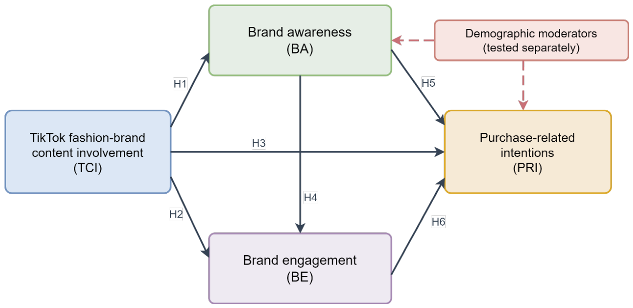
Figure 2.
Proposed human-governed intelligent framework for survey-data analysis.
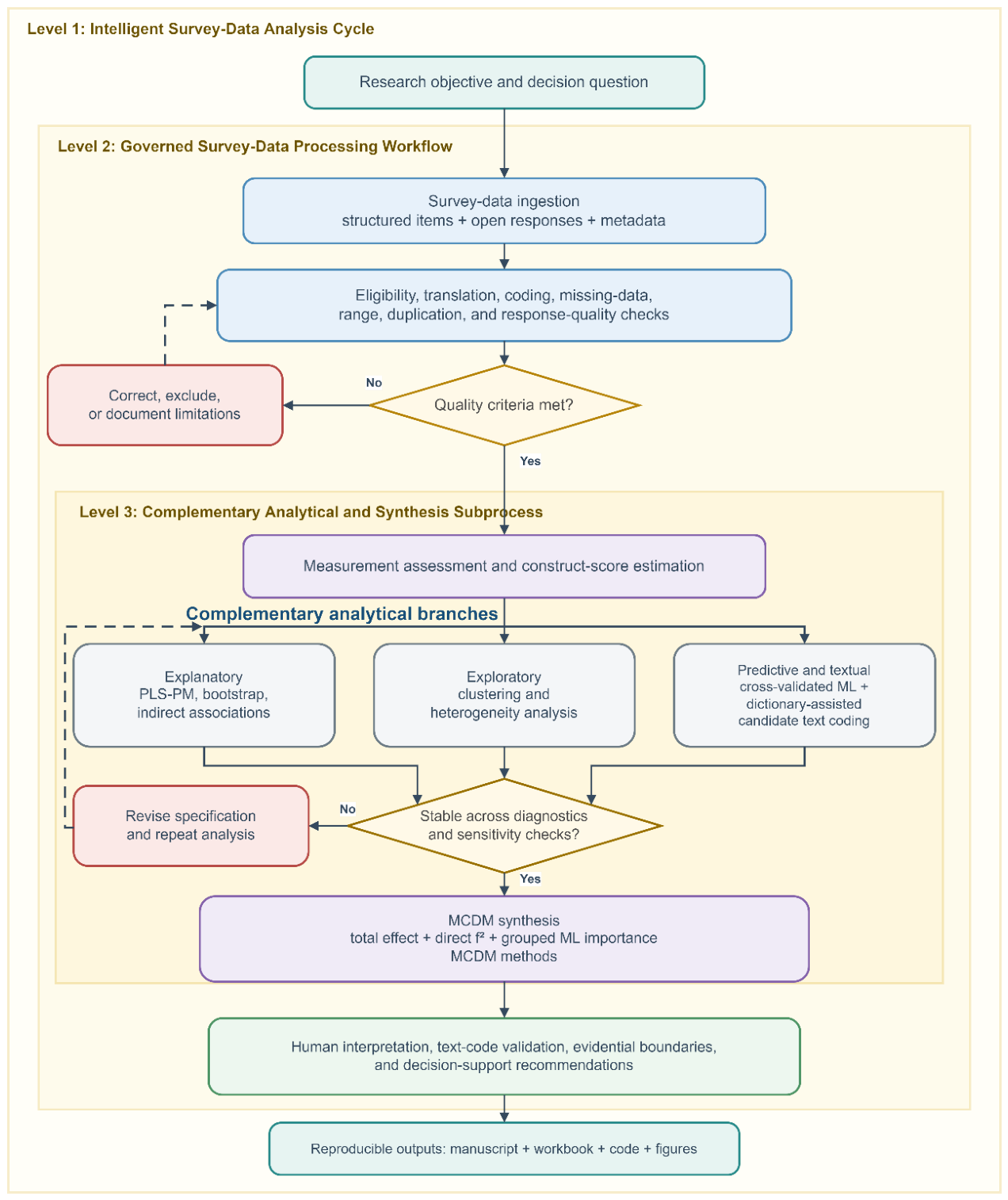
Figure 3.
Respondent-level Euclidean dissimilarity matrix based on the 16 standardized indicators in the principal sample (n = 268). Darker cells indicate greater dissimilarity.
Figure 3.
Respondent-level Euclidean dissimilarity matrix based on the 16 standardized indicators in the principal sample (n = 268). Darker cells indicate greater dissimilarity.
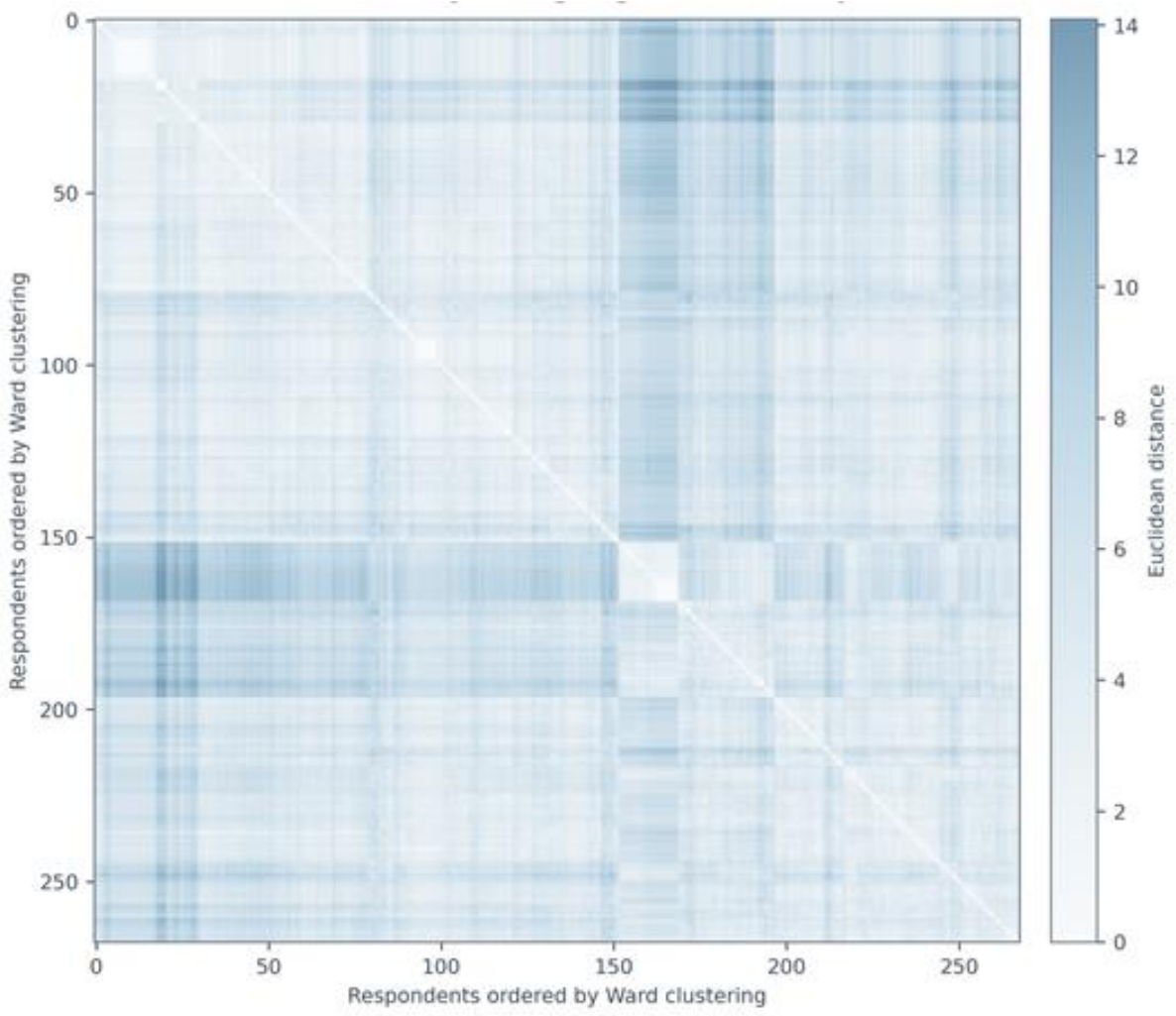
Figure 5.
Ward hierarchical-clustering heatmap of respondents based on the 16 standardized indicators. Dendrogram labels are suppressed because rows represent anonymous response records.
Figure 5.
Ward hierarchical-clustering heatmap of respondents based on the 16 standardized indicators. Dendrogram labels are suppressed because rows represent anonymous response records.
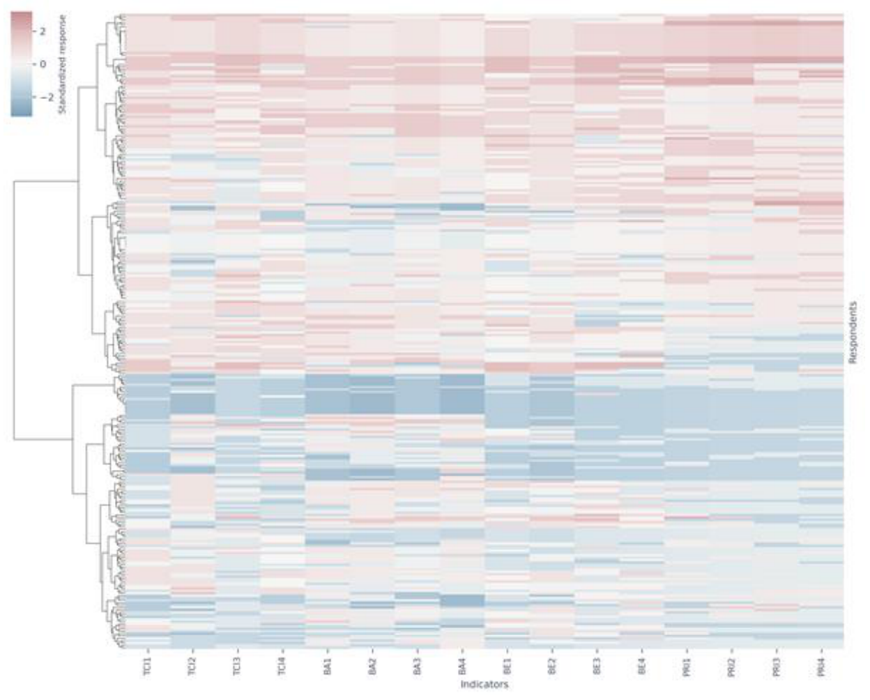
Figure 6.
Ward hierarchical heatmap of the 16 standardized indicators across respondents. The color scale represents within-indicator standardized values.
Figure 6.
Ward hierarchical heatmap of the 16 standardized indicators across respondents. The color scale represents within-indicator standardized values.
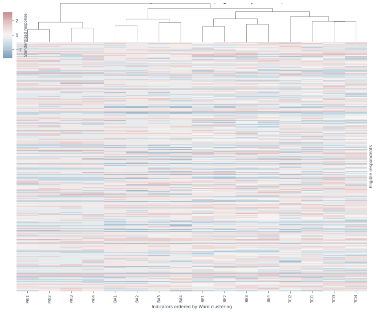
Figure 7.
Principal-component visualization of k-means solutions for k = 2–5. The panels are descriptive projections; cluster selection was based on the full standardized equal-weight TCI, BA, and BE mean-score space.
Figure 7.
Principal-component visualization of k-means solutions for k = 2–5. The panels are descriptive projections; cluster selection was based on the full standardized equal-weight TCI, BA, and BE mean-score space.
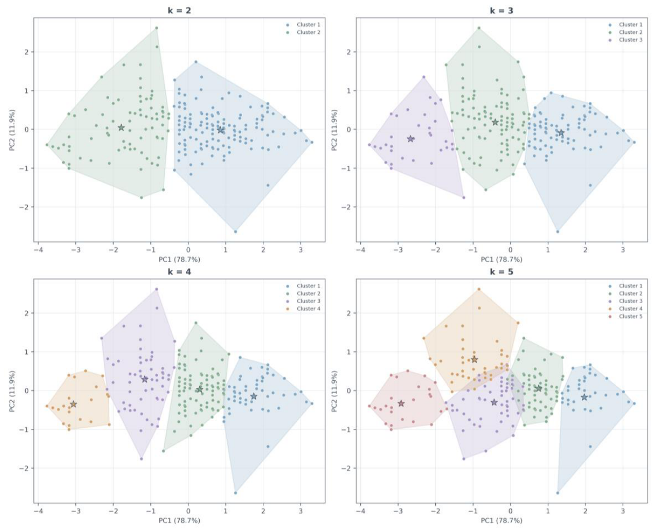
Table 1.
Selected dataset-analysis frameworks and their relevance to intelligent survey-data analysis.
Table 1.
Selected dataset-analysis frameworks and their relevance to intelligent survey-data analysis.
| Framework or approach | Main contribution | Relevance and limitation for survey analysis |
| KDD [13] | Iterative selection, preparation, mining, and interpretation | Provides a knowledge-discovery sequence but does not specify construct measurement or survey-bias diagnostics. |
| CRISP-DM [14] | Business- and data-centered analytical lifecycle | Supports iterative project organization but treats survey measurement and inferential boundaries only indirectly. |
| CRISP-ML(Q) [15] | Machine-learning lifecycle with explicit quality assurance | Strengthens validation and monitoring but is oriented toward ML products rather than mixed explanatory survey studies. |
| ML engineering workflow [16] | Operational tasks surrounding model development and deployment | Emphasizes testing and monitoring but does not integrate latent constructs, group tests, and open-response interpretation. |
| Automated survey-text coding [17,18] | Model-assisted classification and annotation of open responses | Supports scalable text analysis but requires labeled examples, error analysis, and human validation. |
| Proposed candidate architecture | Human-governed coordination of measurement, explanation, exploration, prediction, text analysis, and MCDM | Illustrated for one survey dataset; transferability, comparative efficiency, and external validity remain untested. |
Table 2.
Selected empirical studies on influencer, TikTok, and fashion-related consumer responses.
| Study | Context and method | Main result relevant to this study |
| Lou and Yuan [11] | Social media influencer followers; PLS path modeling | Informative value and source credibility supported trust in branded posts, which was related to awareness and purchase intention. |
| Barta et al. [3] | TikTok influencer marketing | Humor and followers’ hedonic experience were important to influencer-marketing effectiveness. |
| Hazari et al. [4] | TikTok brand influencers; SEM | Brand-influencer impact was associated with prior engagement and purchase likelihood. |
| Gomes et al. [5] | Fashion consumers; mixed methods | Content quality, parasocial interaction, and attitudes toward sponsored posts were related to purchase intention. |
| Alcantara-Pilar et al. [6] | TikTok influencer credibility | Credibility and relational mechanisms were linked to purchase intentions and loyalty. |
| Thuy and Quang [7] | TikTok fashion livestreaming; SEM | Content affected purchase intention directly and indirectly; streamer influence operated indirectly through attitude and trust. |
| Lin et al. [8] | TikTok sustainable-apparel videos | Attitudes toward TikTok videos and sustainable apparel were associated with purchase intention. |
Table 3.
Constructs and measurement items.
| Construct | Code | Abbreviated item content | Specification |
| TikTok fashion-brand content involvement | TCI1–TCI4 | Interest; information sufficiency; sharing with friends; advertising attention | Reflective (Mode A) |
| Brand awareness | BA1–BA4 | Awareness; multimedia information; brand recall; brand recognition | Reflective (Mode A) |
| Brand engagement | BE1–BE4 | Attention; pleasure; user connection; stronger engagement | Reflective (Mode A) |
| Purchase-related intentions | PRI1–PRI4 | Planned purchase; continued purchase; loyalty; recommendation | Reflective (Mode A) |
Table 15.
Inputs to the MCDM synthesis of construct-level analytical relevance.
| Alternative | Total association with PRI | Direct f2 on PRI | Grouped ML ΔRMSE | Quality check |
| TCI | 0.637 | 0.068 | 0.139 | Passed |
| BA | 0.147 | 0.000 | 0.071 | Passed |
| BE | 0.496 | 0.227 | 0.242 | Passed |
Note: The first three columns are benefit criteria. Total association includes direct and estimated indirect structural pathways. ΔRMSE is the deterioration in cross-validated prediction after grouped permutation; a larger value denotes greater predictive contribution. All constructs passed the separate measurement-quality assessment reported in Table 6; this status was not weighted in the MCDM. The values are conditional on the present sample and model.
Disclaimer/Publisher’s Note: The statements, opinions and data contained in all publications are solely those of the individual author(s) and contributor(s) and not of MDPI and/or the editor(s). MDPI and/or the editor(s) disclaim responsibility for any injury to people or property resulting from any ideas, methods, instructions or products referred to in the content. |
© 2026 by the authors. Licensee MDPI, Basel, Switzerland. This article is an open access article distributed under the terms and conditions of the Creative Commons Attribution (CC BY) license (http://creativecommons.org/licenses/by/4.0/).
Copyright: This open access article is published under a Creative Commons CC BY 4.0 license, which permit the free download, distribution, and reuse, provided that the author and preprint are cited in any reuse.