
Submitted:
04 September 2026
Posted:
07 September 2026
You are already at the latest version
Abstract
There exists a huge quantity of papers written about deadlock prevention of Automated Manufacturing Systems (AMS) by means Petri net (PN)-based models in the world literature. In principle they consist in two approaches, namely based either on P-invariants or on siphons of Petri net (PN) models of AMS. The approach presented here makes use of the former approach simultaneously with the structure of deadlocks themselves acquired by means of the reachability tree (RT) of such models. This approach unifies structure of all deadlocks of the AMS PN model as to activity (i.e. operation) places in order to construct the basic matrix [L] used in P-invariant approach making the supervisor synthesis possible. Namely, the product of the matrix [L] with the incidence matrix [N] of the PN model directly yields the incidence matrix [N]s of the supervisor which guarantees deadlock-freeness of the supervised system. In such a way the application of the only one supervisor is able to prevent all deadlocks in the actual model. The approach is verified by means of its application on quite a number of Petri net models of AMS of type S3PR, GS3PR and S4PR. In several cases, the results obtained by the proposed approach are compared with those obtained by the siphon-based approach. The comparison is based on the confrontation of the RTs of supervised models obtained by both approaches. Finally, the possibility of decomposition (or rather splitting) of the supervisor in the case of the structure of very complex S4PR PN models into two supervisors is shown, if in the case of using a single supervisor, the development of one of the two parts of the model (production lines) is suppressed at the expense of the other (as far as access to resources is concerned).
Keywords:
automated manufacturing systems
; discrete-event systems
; deadlocks
; Petri nets
; P-invariants
; resource allocation systems
; siphons
; supervisor
1. Introduction
Discrete event systems (DES) are widely used systems. They cover different kinds of systems in human society. Most widespread are discrete manufacturing systems usually named automated manufacturing systems (AMS), previously named flexible manufacturing systems (FMS). Railways and road transport are also very widespread. Operations accomplished in them (the activity of rail-switches and semaphores, respectively) can also be understood to be a kind of DES. In such complex systems, deadlocks can occur. In AMS deadlocks can lead to a stoppage of production and succeeding economics damages, while in transport even to dangerous disasters with toll of life. Allocation of resources in AMS is the main source of deadlocks. On this account, as to deadlock prevention in them, resource allocation systems (RAS) are the preferred subject of interest in this paper. However, there exists also many other important kinds of DES inside informatics, business, economy, aeronautics, military, etc. Consequently, the deadlock prevention is very important branch of science. Using Petri nets (PN) for modeling DES is very frequent. It has a great advantage that the PN-based models can also be used in different methods for deadlock prevention. Hence, they will also be applied here, in this paper, for both, modeling DES and the deadlock prevention. We are focused here exclusively on deadlock prevention in AMS. In such systems resources are represented by robots, different kinds of machine-tools, buffers, transport belts, automated guided vehicles, etc. Sharing such devices by multiple production lines represents a dominant source of deadlocks in AMS.
1.1. Petri Nets
In principle, from purely mathematical point of view, PNs are a kind of bipartite directed graphs, i.e., graphs with two types of nodes (places and transitions) and two types of edges (directed arcs from places to transitions and from transitions to places). The places (i.e., ), while transitions (i.e., ). Places model particular operations or activities inside of DES. Their states are expressed by marking - i.e., by the number of tokens put into them. Transitions represent discrete events which start or finish these operations.
More precisely, a Petri net can be expressed as where P and T are finite nonempty sets, and ; is the flow relation in N (consisting of flows from P to T and vice versa); assigns a weight to an arc in such a way that if and otherwise. Here, represents the set of integers increased by zero. The net N where , is named as the ordinary Petri net (OPN) . If , the net is named as the generalized net (GPN).
A place in N is marked at marking M if . A place is insufficiently marked with respect to a transition at M if . Here, is the set of output transitions emerging from the place p. If at least one place in a subset is marked at M then S is marked at M. denotes the sum of tokens in all places in S i.e., . If , S is said to be empty at M. If , S is said to be insufficiently marked at M .
A subset is marked by M iff (if and only if) at least one place is marked by M. Thus, represents the sum of tokens in all places in D.
In general, the preset and postset of a node is defined as follows: is the preset of a node , while is the postset of a node .
Let a marked ordinary Petri net is . A transition t is enabled at M, expressed by , if . An enabled transition t at M can be fired. Consequently, a new marking arises. It may be denoted by , where ; otherwise, .
PN marking M is an vector. It is frequently called as the state vector. The evolution of PN marking is performed by means of the following relationship
where is an initial marking, is the incidence matrix, is a vector of non negative integers, called a firing vector. Elements of indicate the algebraic sum of all occurrences of t in . The set of all markings reachable from M by firing any possible sequence of transitions is denoted as . is the set of reachable markings of a Petri net starting from the initial marking .
The equation (1) constitutes the mathematical model of the Petri net N. The matrix is the incidence matrix. It presents the matrix form of the set F. It can also be written in the shape . Finally, is an vector expressing the firing of transitions. It can also be named as the control vector because it represents the state of transitions. When a transition is enabled (i.e., able to be fired) i-th element of the vector is indicated by 1. In the opposite case, when the transition is disabled, it is indicated by 0. Important is to say that the enabled transition may or may not be fired. The marking of a place p is an integer indicating the number of tokens located in this place. The place p is marked by M iff . The mathematical relation ’if and only if’ is expressed by the abbreviation ’iff’ in the whole paper.
A non-empty subset of places is a siphon iff . A non-empty subset of places is a trap iff . A siphon S is minimal iff there is no siphon contained in it as a proper subset. A minimal siphon S is said to be strict if . When a minimal siphon S does not contain a marked trap, it is named to be strict minimal siphon (SMS). Such siphons have to be controlled in order to prevent their emptying.
Siphons are extensively used in a large amount of approaches concerning the deadlock control and liveness-enforcing for both OPN and GPN models of AMSs.
A siphon (trap) S (Q) is said to be empty at marking M iff ().
S or Q is said to be max-marked (min-marked) at a marking M iff or such that , where .
Any PN is deadlock-free when each reachable marking enables a transition, while it is live when each reachable marking enables an occurrence sequence containing all transitions. A transition t is dead [56] in N if no marking of enables t. A deadlock, or dead marking, is a marking enabling no transition. N is deadlock-free if no deadlock belongs to ; otherwise it is deadlockable. The net N is structurally deadlockable if, for every marking M, is deadlockable. A transition t is live in N if for every marking M in , there is a marking in enabling t. N is live if every transition is live in N. N is structurally live if a marking M exists such that is live.
In particular cases, it is possible to prevent deadlocks by a thoughtful change in the system structure. Sometimes even a slight change in the structure of the system itself is sufficient in order to reorganize succession of internal processes in such a way that deadlocks are prevented. However, in systems where the succession of internal processes is strongly prescribed (like in case of technological processes in AMS), supplementing the original structure with an additional structure is necessary. Such a structure is a supervisor, which is designed so that, after connecting to the original system, it is able to guarantee the deadlock prevention in the controlled system.
2. Most Commonly Used Kinds of PN Models of AMS
Mostly used PN models of AMS are Systems of Simple Sequential Processes with Resources (S3PR) and System of Sequential Systems with Shared Process Resources (S4PR).
2.1. S3PR Models of AMS
1) is called the set of activity places (here ∅ means the empty set);
2) is called the idle process place;
3) N is a strongly connected state machine; and
4) every circuit of N contains place .
1. The subnet generated by is an S2P.
2. and .
3. (here represents all input transitions of the place p, represents all input places of the transition t, represents all output transitions of the place p, represents all output places of the transition ).
4. The following statements are verified : (a) and (b) (here is the set of all input places of all input transitions of the place r, represents the set of all output places of all output transitions of the place r).
5. .
Because resources are represented by places from the set , represents input transitions of the resource r. Then is the set of all input places of all input transitions of the place r. Similarly, represents the set of all output places of all output transitions of the place r.
Definition 3 [31,34] Let be an S2PR. An initial marking is called an acceptable initial marking for N if:
(1) ,
(2) , and
(3) . An S2PR with such a marking is said to be an acceptably marked one.
1. An S2PR is an S3PR.
2. Let , be two S3PR such that , and . Then, the net resulting from the composition of and via defined as follows : (a) .
(b) .
(c)
(d) .
(e) is also an S3PR.
In such a way we can compose S3PR by n S2PR. Then if and if , or alternatively, . Transitions in are called source transitions representing raw materials.
Definition 5 [31,34] Let N be an S3PR. is called an acceptably marked S3PR if one of the following statements is true:
1. is an acceptably marked S2PR. 2. , where is an acceptably marked S3PR and
(a) .
(b) .
(c) .
2.2. Generalized S3PR - GS3PR
The difference between S3PR and GS3PR consists in the fact that while S3PR are based on ordinary PN (weights of arcs are only one), GS3PR weights of arcs can be greater than one (i.e., they are based on GPN). Sometimes they are also called [37] weighted S3PR WS3PR. Definitions of them are as follows:
Definition 6 [34,37] A generalized simple sequential process with resources (GS2PR) is a Petri net if:
1. The subnet generated by is an S2P;
2. ( is called a resource or a resource place in the net formalism) and ;
3. , where and , where ;
4. and a unique minimal P-semiflow s.t. , and . Furthermore, ;
5. The following statements are satisfied : and ;
6. .
Definition 7 [34,37] Let be a GS2PR. An initial marking is called an acceptable initial marking for N if ; and .
The couple with N being a GS2PR and being an acceptable initial marking is called a well-marked GS2PR. An acceptable initial marking guarantees that each transition is potentially fireable.
1. A GS2PR is a GS3PR;
2. Let , be two GS3PR such that , and (in this case we say that and are two composable GS3PR). Then, the net resulting of the composition of and via PC (denoted as defined as follows :
(a) ,
(b) ,
(c) ,
(d) ,
(e) ,
(f) is also a GS3PR.
Definition 9 [34,37] Let N be a GS3PR. ) is a well-marked GS3PR if one of the two following statements is true:
1. is a well-marked GS2PR;
2. , where are well-marked GS2PR;
(a) ;
(b) ;
(c) .
Consequently, a GS3PR N composed of k GS2PR can be denoted by , .
2.3. S4PR Models of AMS
More powerful modeling ability than S3PR and generalized S3PR (GS3PR) [34,37] has a class of generalized Petri nets named as S4R [35]. In the sense of [33] S4PR are equivalent to S4R.
Definition 10 [33,34] A well-marked S4R net ) is a marked Petri net with initial marking such that :
1. is a partition such that
(a) is called the set of activity places, where and .
(b) is called the set of idle places.
(c) is called the set of resource places;
2. . ;
3. , where and , and ;
4. generated by is a strongly connected state machine such that every circuit in contains place ;
5. , there exists a unique minimal P-semiflow such that , and . Furthermore, we have ;
6. N is pure and strongly connected;
7. , and .
2.4. Brief Summary
It can be said that GS3PR is a subclass of S4R (or S4PR) and a generalized version of a S3PR. A GS3PR is equivalent to WS3PR. An activity place representing a processing stage of a job needs a single unit of a single resource type. The usage of resources in S4R is almost arbitrary and requires only conservativeness.
Theorem 1 [38] A Petri net N is (partially) conservative iff there exists an vector y of positive (nonnegative) integers such that .
3. Using Knowledge of Deadlocks in the Reachability Tree of PN Model to Form a Procedure for Themselves Prevention in that Model
Just as siphons form a kind of a substructure in a Petri net, and similarly P-invariants and T-invariants form another substructures of PN, deadlocks also form a kind of substructure of PN. It results from the reachability tree (RT) the nodes of which are being PN reachable markings (i.e., states of PN). Deadlocks are unambiguously determined as a part (a subset) of RT nodes, because RT is unambiguously determined for any PN. Since, to each PN belongs the only one RT, deadlocks that clearly belong among these nodes of the RT (they are some of PN states at which no transitions can be fired, i.e., they are unwanted terminal states), also have an important informative value about the PN. Let us utilize this as a kind of a hypothetical feedback in the process of deadlock prevention. It may sound indeed paradoxical, but let us use the knowledge of deadlocks obtained from the RT of the PN to prevent deadlocks themselves in this PN. However, the question arises as to how to implement this.
This paper presents an unusual approach to the deadlock prevention in Petri net based models of AMS. Namely, there exist two main approaches to the PN deadlock prevention in the world literature. There are based either on (i) P-invariants; or on (ii) siphons. In both areas a galaxy of literature were written. The invariant-based approach is touched especially in [9,10,12,26,32,41], while the siphon-based approach is presented in [2,3,4,5,6,7,8,14,18,19,20,21,22,23,24,29,30,31,33,34,36,37,40,45,47]. A brief introduction to both approaches was presented in [2].
In this paper we will be based especially on [13,15,27,39,46,48,49,50,51,52,53] as well as on PN theoretical works [16,17,28,38,42,43,56] and on PN practical works [25,26] concerning the GPenSIM editor for Petri nets.
The PN models of AMS contain three groups of places (as it was introduced in Section 2) idle, activity and resource places. The approach that will be presented here, is based on the approach based on P-invariants, but it modifies the choice of elements for the matrix (see below introduced relationships (7) - (15)), which plays a significant role there. It represents prescribed conditions in the inequality (7).
In our approach is characteristic the specific procedure for creating the matrix . It is based on a sort of aggregation of activity places occurring in PN deadlock markings (i.e., in RT nodes, being PN state vectors, representing deadlocks) and their incorporating into the matrix as its elements. This operation brings information about deadlocks and their mutual interconnections to the method based on P-invariants. At creation of idle places and resource ones are not used. Namely, it can be said that on the one hand idle places do not affect significantly (the sufficient amount of them is put from outside by the plant operator) the internal structure of deadlocks and, on the other hand, resources are not affected by deadlocks because their amount depends on outside appearances (they are given also from outside). Though a lack of resources can cause deadlocks, but it cannot solve them. Activity (i.e., operation) places present a core of events inside the production processes. Setting the marking of idle places and resource places is an external matter.
3.1. A Short Consideration about Deadlocks
Deadlocks are structural parameters of Petri nets. They are unwanted in real AMS as well as in their PN models. A deadlock occurs there when the system reaches a state where no PN transitions can be fired. The system halts its operation and further continuation of the activity is impossible. When we are trying to find a mutual relations among deadlocks in a Petri net we hit on the answer that the analysis of its reachability tree (RT) is the closest way how to achieve this. Namely, to a PN appertains unique RT. However, the opposite is not true. RT nodes yield particular states of PN, i.e., the whole state space, including deadlocks. It can therefore be assumed that knowledge of deadlocks can be retroactively utilized to influence the structure of the PN. Let us try to use deadlocks for changing the structure of the original PN to remove them, i.e., for finding a supervisor realizing the deadlock prevention in the original PN. It will be performed in further Sections.
3.2. Multisets vs. Sets
It is usual to express PN states by means of multisets in the sense of the definition originally introduced in [40]. A multiset is a generalization of the concept of a set. A multiset , over a non-empty set A, is a mapping , which we represent as a formal sum . For example, when the PN marking (i.e., state) we will write as . For two multisets is valid the following: and .
3.3. A Simple Example of S3PR PN Model of AMS
Let us find a supervisor that has to be added to the original deadlocked system being the S3PR modeled by PN displayed in Figure 1 left, and which will control it in such a way that deadlocks cannot occur. Its RT in this Figure right shows us that there exists only one deadlock.
Let us compare both the siphon based approach to the deadlock prevention and the approach based on activity places contained in deadlocks in RT (i.e., being familiar with all its nodes representing whole state space including deadlocked states).
The state space of the system is given by the RT nodes in the form of row vectors as follows.
The RT shows us that the node is the deadlock. The incidence (structural) matrix of the system is the following
Let us compare the siphon-based approach (see e.g., [2,3,4]) to the deadlock prevention with the deadlock prevention proposed in this paper. It is necessary to show that the RT-based approach, more precisely the deadlock-based approach in our case, is also sound.
3.3.1. Siphon Based Approach
First let us use the elementary siphon based approach to the deadlock prevention. Almost all articles referred to in this paper are interested in the siphon-based approach at the deadlock prevention except [11,27,32,39,41]. There is only one elementary siphon in the system, namely
Hence, the incidence matrix of the supervisor is as follows
It means that we can use the new Petri net structure containing the place with marking being the supervisor. It is connected with the original structure in such a way that interconnections from direct to transitions and while interconnections to direct from transitions and . Thus, the new structure is displayed in Figure 2 left while RT is presented in Figure 2 right to document deadlock-freeness of the supervised plant. In this way we can see that no deadlock occurs in the united structure.
3.3.2. Proposed Approach
Note that the deadlock (node ) contains two activity (operation) places and . Create the matrix using these places, i.e., . Try to put . We obtain . We can see that the supervisor is the same like that in (5).
Such approach was not applied just like haphazardly, of course. It follows from the P-invariant based approach to the deadlock prevention introduced below, where the matrix is composed by means of the activity places contained in the marking representing the deadlock. It was shown here that the activity (operation) places contained in deadlocks (i.e., in RT nodes expressing deadlocks) have an impact on the prevention of themselves. In this simple example even they give the same results as elementary siphons.
Consequently, it can be said that there exists a certain feedback effect of RT on PN itself, although in general it may not be as unambiguous as is the relationship from PN to RT. On the other hand, it should also be added that it cannot be expected that the results of applying this approach will generally be identical to the approach based on siphons.
4. P-invariant Based Approach to Deadlock Prevention in General
Let us first look at the problem of deadlock prevention from the P-invariant point of view, which is the basis of the proposed approach.
Definition 11 [2,11,32,41] A vector I is a place invariant P (shortly, P-invariant) of PN iff and . Here, is the incidence matrix of N.
Definition 12 [31] A siphon S in an ordinary PN is invariant controlled by P-invariant I under the initial marking iff and , or equivalently, and is the positive support of I.
For P-invariant I it holds [2,11,32,41] the relation of the state conservation, as follows
The following inequality representing linear combinations restricting behavior of marking M is important for the deadlock prevention based on P-invariants. Let the following inequality holds
Here is a matrix of integers, M is a PN marking vector and b is an integer vector. To remove the inequality we can add slack variable s. Thus we have
where s is vector of integers.
When we force instead of into (see the Definition 1), we obtain
where is -dimensional identity matrix; is the number of slacks; is a -dimensional matrix of integers; is the PN incidence matrix; is the -dimensional matrix of integers, and m is the number of PN transitions. Thus, after finding from (9), we obtain the incidence matrix describing the structure of the PN-based model of the supervisor.
Consequently,
where is and is of .
Marking of the supervised system will consist of marking M of the original (unsupervised) system and marking of the supervisor , i.e., . Therefore we can write
Consequently,
Thus, there is the only freedom of choice, namely the suitable choice of the structure and elements of the matrix which the only are at the disposal for experiments. The reachability tree (RT) of the net N yields an efficient help at creating . RT nodes are state vectors (markings) of PN. These states include among themselves also PN deadlocks (dead states). The proposed method just uses the places of deadlock markings that correspond to activity (operation) places of the PN. Namely, just these places represent production processes inside AMS.
In [47] the RT nodes are divided (as to marking) into four categories: good, dangerous, bad, and deadlock markings. At formulation of our approach, the partial knowledge from [12,13,45,46] was utilized, especially those concerning the isomorphism of graphs and isomorphism of PNs. The graph isomorphism problem is the computational problem of determining whether two finite graphs are isomorphic.
Definition 13 [46]: Let and be two directed graph, where and indicate the vertex and edge sets, respectively. Suppose that there is an isomorphism between and , which is denoted as , such that there exist two functions and .
Definition 14 [53] Given two graphs and an isomorphism between G and H is a bijection satisfying for every pair of nodes , .
And even automorphisms in is the set of bijections from onto itself satisfying .
These definitions can be applied to PN model, which is also a class of directed graphs (namely, bipartite directed graph). In [46] were proved the next Theorems, where authors lean on the algorithm ’Think-globally-act-locally’, presented in [45]:
Theorem 2 [46]: Given two PN models and . Let their vertex sets be and edge sets be . If there are two bijective functions and , it is verified that .
Theorem 3 [46]: Given two isomorphic PN models and with the same initial marking . It is said that the related reachability graphs and also have isomorphism relationship, where .
Already more then 60 years ago in [48] a heuristic algorithm was proposed for testing pairs of directed line graphs for isomorphism. However, till now it is not known the problem to be solvable in polynomial time, however nor to be NP-complete, and therefore may be in the computational complexity class called as NP-intermediate. Relatively new research in this area was published in [49]. In [50] a category of nested-unit PN (NUPN) were defined in order to study PN isomorphism. A quasi-polynomial ( where n is th number or graph vertices) algorithm for isomorphism of graphs was published in [51]. Isomorphism in connection with parallel processing of calculations, or rather the number of parallel processors required, was addressed in the work [53].
4.1. Creating the Matrix
In order to obtain elements of the integer matrix an aggregate of markings of activity places has to be created. We start from RT nodes corresponding to deadlocks (occurring among PN state vectors). Such an aggregate, the set S, consists of the union of subsets , where is the number of deadlocks
Suppose that there are activity places in the PN. Of course, these places don’t have to be consecutive. In particular deadlocks they occur together with their markings , being greater or equal to zero. Then,
corresponds to the deadlock . Namely, in different deadlocks these places are presented with different markings. Elements of the set S are just derived from markings of corresponding activity places. Namely,
Thus, such aggregated markings of activity places are then becoming the corresponding elements of the matrix . It means that to the zero matrix (n is the number of PN places) we insert the aggregates of markings which correspond to activity places and remaining elements of stay zeros, because we do not consider them. Thus, the elements of :
where and are, respectively, the set of zero elements in positions of idle places and that in positions of resource ones. However, it should be emphasized here, that the arrangement of these elements in the matrix depends on the numbering of places in the investigated PN. Therefore, the elements of the matrix have to be aligned in the same order, i.e., succession of idle, activity and resource places need not be consecutive (i.e., can be mixed), because the order of elements in deadlocks also depends on the numbering of places in the investigated PN. The important thing is that all elements of the matrix , except those corresponding to activity places, are zero. This is also presented in several examples (even, may be said the whole series) introduced in next Sections of this paper.
Finally, we find (in the sense of (11) the incidence matrix of the supervisor as follows
In next Sections are introduced examples verifying correctness of the proposed approach to the deadlock prevention.
5. Verification of Proposed Approach
In this section several case studies of the kind of S3PR, GS3PR and S4PR PN models of AMS.
5.1. AMS Modeled by Generalized Petri Nets
Consider the S4PR PN model of a simple manufacturing system in Figure 3 consisting of two subsystems (subnets) sharing two resources.
The RT nodes are represented by the state vectors as follows
The supervised system, where the supervisor computed by another method for generalized PN (see e.g., that in [4]), is presented in Figure 4 left while its RT is right.
When in Figure 4 we put marking and when we assign the weight of the arc as we obtain also the resulting deadlock-free system, only RT will be displayed in Figure 5.
5.1.1. Proposed Aproach
The RT node
is the deadlock. It contains two activity places and . After their projection into the matrix we have the matrix
.
Consequently, we obtain the incidence matrix of the supervisor
.
With respect to (12) negative elements belong to while the positive ones belong to . Hence, PN arcs from the supervisor lead to the transitions and while arcs from transitions and arrive to the supervisor. The supervised system is displayed in Figure 6 left while its RT documenting the deadlock-freeness is right.
5.2. Another GS3PR PN Model of AMS
Consider the GS3PR model in Figure 8.
The PN model has the following incidence matrix
5.2.1. Siphon Based Approach to Deadlock Prevention
There is only only one siphon in the PN model. It is the following
The supervisor incidence matrix is the following
The supervised system is in Figure 9 left, with the supervisor depicted in red, while the RT documenting the deadlock-freeness is right.
5.2.2. Proposed Approach Resolving the Problem
As we can see in RT of the PN model in Figure 8 (see also the list of its nodes below) there is the deadlock .
Respecting activity places only (finally, this deadlock does not even contain other places), N12. Consequently we can put
.
The incidence matrix of the supervisor is
.
Then the supervised system is in Figure 10 left together with its RT right. The supervisor is depicted in red. RT shows that no deadlock is in the supervised system.
5.3. Slightly Larger S3PR and GS3PR PN Models
In this case as well as in further cases, we will not already introduced the siphon-based approach in order not to unnecessarily increase the scope of the article.
5.3.1. S3PR PN Model with Minimal Resources
Consider S3PR model of a simple AMS displayed in Figure 11. Similar model was solved in [4] using the siphon-based approach.
The transpose of its incidence matrix () is expressed in the form of the table in Figure 12
The RT of this PN model is depicted in Figure 13. It documents existence of two deadlocks in the PN model - nodes .
As we can see in the RT there are two deadlocks in the uncontrolled PN model:
Consider deadlocks
.
Hence, we can see that we have two sets of activity places and . After their union we have the set . Hence, we can create the matrix in the form
and applying (12) we have the incidence matrix of the supervisor
The supervised system is displayed in Figure 14. Its RT is in Figure 15. The RT documents that there are no deadlocks in the supervised model.
Let us compare figures Figure 14 and Figure 15 on the one hand with results (presented in [4]) displayed in Figure 16 on the other hand. There are 3 supervisors synthesized by the method based on siphons in Figure 16 on the left and the corresponding RT of the controlled model on the right which has 14 nodes. It is clear that we have achieved here, in this paper, the RT (in Figure 15) which on the one hand has indeed only 10 nodes and is a little bit less branched, but on the other hand these results were achieved by the single supervisor only.
5.3.2. A GS3PR Model described by Generalized PN (GPN)
Consider the GPN model displayed in Figure 17.
Its RT has 38 nodes (consequently, it cannot be introduced here) and it points out two deadlocks
and
.
Their unifying gives us , hereof
and
.
The supervisor structure is displayed in Figure 18 left. The RT of the supervised GPN model is displayed in the same figure right. It can be seen that there is no deadlock in the RT.
5.4. Simple S4PR GPN Model
Let us use the S4PR GPN model displayed in Figure 19.
This PN model of AMS has RT with 21 nodes. Hence, it cannot be introduced here. There is one deadlock in this model - the node
N9 = .
Consequently,
.
The supervisor
.
The supervised system has RT with 16 nodes. The supervised system is displayed in Figure 20 up, while the RT documenting deadlock-freeness of the controlled model is displayed down.
5.5. Further S4PR PN Model
Consider the S4PR PN model and its RT in Figure 21. The RT points out to two deadlocks
and
what leads to two subset of activity places and . Hence,
.
Consequently,
.
The supervised system is in Figure 22 (left) with the supervisor displayed in red, and its RT (right) documenting deadlock-freeness.
The alternative siphon based approach leads to 6 siphons what complicates the supervisor synthesis.
5.6. Another S4PR PN Model
Consider the deadlocked S4PR PN model with the structure displayed in Figure 23 (left) together with its RT (right).
As we can see there are not only two deadlocks but also a dwarfism of the state space. The transpose of the incidence matrix of the S4PR PN model is given in Figure 24.
The RT points out to two following deadlocks:
Node 3:
Node 4:
Ignoring idle places we can see that in the former node there is the activity (operation) place while in the latter node the operation places . When we unify them into one set we can construct the matrix
.
Consequently, we can find the incidence matrix of the supervisor as follows
.
Applying the supervisor into the original PN model we obtain the controlled structure and RT documented its deadlock-freeness in Figure 25.
5.7. GS3PR PN Model with a More Complex Structure
Let us consider the PN model of an automated manufacturing system in Figure 26. Its transposed incidence matrix is displayed in Figure 27 in the form of a table.
The RT of the GS3PR PN model has 247 nodes. Consequently, it cannot be displayed here. There are five deadlocks in it as follows:
Taking only operation places into account in particular deadlocks we have following subsets of such places; . The union of these subsets has the form . Taking into account corresponding markings of these places in particular deadlocks, we obtain the matrix:
and the supervisor
displayed in Figure 28 where the supervisor consists of the place with corresponding directed arcs (with corresponding weights) to transitions of the original PN model and directed arcs (with corresponding weights) from transitions back to the supervisor. The marking of the place is .
5.8. Another S4PR PN Model
Consider another S4PR PN model displayed in Figure 29. Its RT is in Figure 30 where one deadlock occurs:
.
Corresponding activity places are , hence
and the supervisor
.
The supervisor is displayed in Figure 31 left, while the RT documenting the deadlock-freeness of the supervised system is right.
The supervisor is displayed in Figure 31 left in red, while the RT of the supervised system is right. The RT shows that the supervised model is without deadlocks.
6. Large-Scale S3PR PN Model
Consider the S3PR PN model displayed in Figure 32. There can be seen that the model is relatively large-scale because it consists of 4 cooperating production lines. Correct coordination of them is not easy, and less so the deadlock prevention. Nevertheless, the approach presented here, offers effective solution.
Here, the places are idle places and are resources that all 4 production lines compete (or bid) for. RT of this model has 1144 nodes but 6 of them are deadlocks:
Here we have the following sets of activity (operation) places: , , , , , . When we apply the union of these sets of operation places (i.e., without idle and resource places) from these deadlocks we obtain the set
,
and so we can create the matrix
and consequently the incidence matrix of supervisor
The supervisor is depicted in Figure 33. After applying this supervisor to the PN model we obtain the system with 653 states but without deadlocks. This was verified by means of the above mentioned GPenSIM tool [14,26] in Matlab. Authentic behavior of the supervised model can be verified by simulation in any respectable PN editor.
7. S4PR PN Models with More Complicated Structure
Here, two relatively complex S4PR PN models are introduced. In the second model will be shown that in case when we are not satisfied with the behavior of the supervised system we can apportion the matrix with one row into the matrix with two rows.
7.1. Example 1
Consider S4PR PN model of AMS in Figure 34.
Eliminating idle places we have two subsets of places in particular deadlocks are and . After using the union operation on them we can find and consequently, the matrix
.
Then, the incidence matrix of the supervisor is
.
The supervisor is displayed in Figure 35. The supervised system has RT with 305 states and it has no deadlocks. The authentic behavior of the controlled model can be verified in any serious PN editor.
7.2. Example 2
Consider another S4PR PN model with significantly complicated structure displayed in Figure 36.
This example was resolved by the siphon-based approach in [21], more precisely said by so called augmented elementary siphons. There, the supervisor consists of 7 elements.
Here, we have 16 142 nodes in the RT (computed by GPenSIM tool [14,26]) of the uncontrolled model in Figure 36, including 10 deadlocks as follows:
N2466: (5 1 3 0 1 0 8 2 0 0 0 0 0 0 0 0)
N3166: (5 2 2 1 0 0 7 2 0 1 0 0 0 0 0 0)
N4845: (5 2 2 0 1 0 7 2 0 0 1 0 0 0 0 0)
N5741: (5 3 1 1 0 0 6 2 0 1 1 0 0 0 0 0)
N6621: (6 1 3 0 0 0 5 2 0 3 0 0 0 0 0 0)
N7639: (5 3 1 0 1 0 6 2 0 0 2 0 0 0 0 0)
N8555: (5 4 0 1 0 0 5 2 0 1 2 0 0 0 0 0)
N9466: (6 2 2 0 0 0 4 2 0 3 1 0 0 0 0 0)
N11909:(6 3 1 0 0 0 3 2 0 3 2 0 0 0 0 0)
N13792:(6 4 0 0 0 0 2 2 0 3 3 0 0 0 0 0)
and consequently we have following set of activity places (i.e., exclusive of idle places and resources) as follows: , , , , , , ,
, , .
Using union operation on these subsets we can find the set
,
and consequently the matrix
.
After performing the operation , we obtain the supervisor incidence matrix in the form
.
The supervisor is displayed in Figure 37.
The supervised system has RT with 47 states and it is without deadlocks.
Applying this supervisor into the unsupervised system in Figure 36 we indeed achieve the deadlock-free system, however its behavior is not satisfied. The right part (right subsystem) of the system is developed intensively while the left one very modestly, almost at all. The controlled system development is too asymmetrical. It is undesirable situation.
Fortunately, we found the interesting way how to resolved such a problem, namely by a decomposition of the supervisor into two ones as follows. The decomposition consists in splitting the matrix into two portion and create the new matrix with two rows. In our case into the first row of the new matrix we put first eight elements of and other eight elements we put zeros. Into the second row of the matrix we put first eight elements zeros while into the second eight elements the second eight elements of original matrix . In this way we have obtained the following matrix. Let us name it repeatedly .
Consequently,
Thus, we have two supervisors given in Figure 38. Applying them to the original unsupervised system we obtain deadlock-free system with the RT having 1028 states (computed by GPenSIM tool [14,26]). These two supervisors cover the same transitions like the original single supervisor. The second supervisor is quasi wrested out of the original supervisor in Figure 37. It should be noticed that after some fictitious optical identification (reverse composition or reassembling) of both supervisors in Figure 38 (i.e., amalgamating supervisors and into one) we get formally the original single supervisor in Figure 37. However, while the single supervisor yields only 47 states of the supervised system, applying two supervisors yields 1028 states and more satisfying behavior. Simulation on any serious PN editor shows that while in the former case the behavior of the supervised system is not satisfied, in the latter case it fully meets the needs. But for calculating RT, the GPenSIM tool [14,26] is suitable, especially in case of huge amount of nodes. It offers results relatively quickly - all RT states including deadlocks in the form of multisets (see Section 3.2) and integers of nodes being deadlocks.
8. Large-Scale S4PR PN Model of AMS
Consider large-scale S4PR PN Model of AMS in Figure 39. It was resolved in [46] by another approach.
It has 23 places and 18 transitions. Transpose of its incidence matrix is given in Figure 40 in the form of the table.
According to our calculations, the RT model has 19,299 nodes. Among them there are 25 deadlocks. The list of these deadlocks is introduced there, in [46]. Here, they are introduced in the Table 1.
Let us apply our approach to resolve that problem, i.e., to synthesize a supervisor realizing the deadlock prevention for that PN model. Utilize the list of deadlocks to create subsets of activity places corresponding to those deadlocks. They are introduced in Table 2.
Here, are idle places and are resources. Applying the union relation on the subsets introduced in Table 2 we have
Thus, we can write the matrix:
and to obtain the incidence matrix of the supervisor
.
Applying such supervisor into the original uncontrolled system we obtain system without deadlocks. The supervisor is displayed in Figure 41. Number of RT nodes of the controlled system is 299.
Verifying behavior of the system controlled by this supervisor on a PN editor shows the balanced deadlock-free development of its subsystems. In [46], where the problem was resolved by another way, another supervisor was obtained. The RT of the supervised system in that case has 270 nodes and the system is deadlock-free.
9. Results
The method for deadlock prevention based on P-invariants but with the specific construction of the matrix incident in relationships (7)-(15) was proposed and verified on several examples of S3PR, GS3PR, and S4PR. In SubsubSection 5.1.1, in SubsubSection 5.2.1, and in SubsubSection 5.2.2 the proposed approach was tested on relatively simple GPN models. In the SubsubSection 5.3.1 we tested the S3PR PN model with strictly minimal resources. Obtained results were compared with results obtained at solving the same model resolved in [4] by the siphon-based approach. A GS3PR PN model was presented and resolved in SubsubSection 5.3.2. In the SubSection 5.4, in the SubSection 5.5, and in the SubSection 5.6 S4PR PN models were introduced and resolved as to deadlock prevention. In the SubSection 5.7 a GS3PR PN model with more complex structure was resolved. In the SubSection 5.8 the S4PR PN model was resolved.
In the Section 6 the large-scale S3PR PN model was resolved and finally, in the Section 7 two S4PR PN models with more complicated structures were resolved in the Example 1 in SubSection 7.1 and in Example 2 in SubSection 7.2, respectively. In the latter example the matrix were rebuilt from the one-row matrix into the matrix with two rows in order to ensure not only the deadlock-freeness but also a symmetry of development of both subsystems (left and right) of the supervised model.
Thus, an important result was achieved. Namely, when the single supervisor based on the one-row matrix accomplished deadlock-freenes but it does not satisfy the expected quality of the controlled system behavior, it can be decomposed into two (in general more) supervisors (or better said we can create the two-row or, in general multi-row, matrix ).
In such a way built supervisors achieve together not only deadlock-freeness but also better behavior of the controlled system. The research in this direction seems to be promising. However, such research may be time-consuming for experiments, especially in case of many deadlocks.
In the Section 8 our proposed approach is applied on the large-scale S4PR PN model presented in [46]. The model is displayed in Figure 39 and the transpose of incidence matrix in the model is displayed in Figure 40. This S4PR PN model has RT with 19 299 nodes inclusive of 25 deadlocks. After finding the supervisor displayed in Figure 41 and its application on the original model we obtain deadlock-free system having RT with 299 nodes. The supervisor found in [46] is different. After its applying on the original model the supervised system has 270 states and it is deadlock-free too. Both of supervised models were verified by simulation in a PN editor.
10. Discussion
In this paper we present the simple effective method for deadlock prevention of S3PR, GS3PR, and S4PR Petri net models of AMS. It present a novelty at the construction of the matrix prescribing the set of constraints in the P-invariant based method of deadlock prevention for PN models of AMS presented in Section 4. As elements of the integer matrix an aggregation of activity places , occurring among PN state vectors, being nodes of RT corresponding to deadlocks, are inserted. More details are introduced in SubSection 4.1.
The proposed method was successfully examined on a number of varied kinds and different sizes of PN models of AMS. Compared to other methods, this method appears to be effective and relatively simple to be promising. From a formal point of view, this method is a form of a feedback between the reachability tree of a deadlocked Petri net and the structure of the net itself. The result of such feedback yields the supervisor ensuring the deadlock-freeness of the net controlled by it. It may seem to be paradoxical, but knowledge of deadlocks (namely marking of their activity places) obtained from the deadlocked RT nodes of the Petri net is, contrarily, used at computing the supervisor ensuring the deadlock-freeness of the net. 253 PN to prevent deadlocks themselves in this PN.
11. Conclusions
The deadlock prevention of AMS represents very wide area of research. Accordingly, there exist many directions of development of methods in both in theory and in applications. Two directions leave the most distinctive and noticeable mark on this way. They are approaches to deadlock prevention based on P-invariants and those based on siphons. This paper was devoted to a contribution to former direction. It brings an approach to creating the integer matrix which represents a key element (core) of the approach based on P-invariants. Elements of are derived from deadlocks themselves obtained from the reachability tree of the Petri net, which is just to be investigated as to deadlock prevention. Namely, markings of activity places occurring in particular deadlocks are unified into an aggregate and consequently create . After multiplying the PN incidence matrix by the matrix from the left we obtain the supervisor . Applying such supervisor on the PN ensures the deadlock-freenes of the PN. Normally we make do with the single-row matrix . However, in case of too structurally complex AMS, as it was shown in the Example 2 in the Section 7, when we are not gratified with the behavior of the supervised PN we can decompose the matrix into a double-row matrix. This topic seems to be interesting as to further investigation.
Funding
This research received no external funding.
Data Availability Statement
Data are contained within the article.
Acknowledgments
This work was partially supported by the Slovak Grant Agency for Science VEGA under Grant No. 2/0005/25.
Conflicts of Interest
The author declares no conflicts of interest.
Abbreviations
The following abbreviations are used in this manuscript:
| AMSs | Automated Manufacturing Systems |
| DESs | Discrete-Event Systems |
| FMSs | Flexible Manufacturing Systems |
| PNs | Petri Nets |
| RASs | Resource Allocation Systems |
| OPNs | Ordinary PNs |
| GPNs | Generalized PNs |
| S3PRs | Systems of Simple Sequential Processes with Resources |
| ES3PRs | Extended S3PRs |
| GS3PRs | Generalized S3PRs |
| S4Rs | Systems of Sequential Systems with Shared Resources |
| S4PRs | Simple Systems of Simple Sequential Processes with Resources |
| WS3PRs | Weighted System of Simple Sequential Processes with Resources |
References
- Liu, G. Complexity of the deadlock problem for Petri nets modeling resource allocation systems. Inf. Sci. 2016, 363, 190–197. [Google Scholar] [CrossRef]
- Čapkovič, F. Dealing with Deadlocks in Industrial Multi Agent Systems. Future Internet 2023, Vol. 5(No. 3, 107), 1–25. [Google Scholar] [CrossRef]
- Čapkovič, F. Sustainability of Automated Manufacturing Systems with Resources by Means of Their Deadlock Prevention. Electronics 2024, Vol. 13(No.17), 3517. [Google Scholar] [CrossRef]
- Čapkovič, F. Siphon-Based Deadlock Prevention of Complex Automated Manufacturing Systems Using Generalized Petri Nets. Electronics 2025, Vol. 14(Issue 24), 4889. [Google Scholar] [CrossRef]
- Bérard, B.; et al. Deadlock-freeness. Chapter. In Systems and Software Verification; Springer: Berlin, Heidelberg, 2001; pp. 99–101. [Google Scholar] [CrossRef]
- López-Grao, J.-P.; Colom, J. M.; Tricas, F. Prevention Policies for Flexible Manufacturing Systems A Petri Net Outlook. Chapter 7. In The Book Formal Methods in Manufacturing, First Edition 2014; Campos, J., Seatzu, C., Xie, X., Eds.; CRC Press, Taylor and Francis Group: Boca Raton, London, New York, 2014; pp. 197–227. [Google Scholar] [CrossRef]
- Cano, E. E.; Rovetto, C. A.; Colom, J.-M. An Algorithm to Compute the Minimal Siphons in S4PR Nets. IFAC Proc. Vol. 2010, Volume 43(Issue 12), Pages 15–20. [Google Scholar] [CrossRef]
- López-Grao, J.-P.; Colom, J.-M. Resource Allocation Systems: Some Complexity Results on the S4PR Class. In Proceedings of the 26th IFIP WG 6.1 International Conference Formal Techniques for Networked and Distributed Systems FORTE 2006; Paris, France, Najm, E., et al., Eds.; 2006; LNCS Vol. 4229, pp. 323–338. ISBN 978-3-540-46219-4. [Google Scholar] [CrossRef]
- Memmi, G. Home Spaces and Invariants to Analyze Parameterized Petri Nets. 20 pages. 2024, arXiv:2403.11779v1 [cs.DM] 18 Mar 2024, 20 pages. [Google Scholar] [CrossRef]
- Memmi, G. Invariants and Home Spaces in Transition Systems and Petri Nets. 108 pages. 2024, arXiv:2306.07623v4 [cs.FL] 21 Oct 2024, 108 pages. [Google Scholar] [CrossRef]
- Iordache, M.V.; Antsaklis, P.J. Supervisory Control of Concurrent Systems: A Petri Net Structural Approach; Birkhäuser: Basel, Switzerland, 2006. [Google Scholar] [CrossRef]
- Lee, S.-C.; Cheng, J.-F.; Row, T.-C. Deadlock Prevention Policy for Flexible Manufacturing Systems: Petri Net-Based Approach Utilizing Iterative Synthesis and Places Invariant. Eng. Proc. 2025, 108, 37. [Google Scholar] [CrossRef]
- Row, T.-C.; Pan, I.-L. Incomparable Single Controller for Solving Deadlock Problems of Flexible Manufacturing Systems. IEEE Access 2023, Vol. 11, 45270–45278. [Google Scholar] [CrossRef]
- Chen, I.F.; Li, Z.W.; Zhou, M. C. Behaviorally Optimal and Structurally Simple Liveness-Enforcing Supervisors of Flexible Manufacturing Systems. IEEE Trans. Syst. Man. Cybern. — Part A Syst. Hum. 2012, Vol. 42(No. 3), 615–629. [Google Scholar] [CrossRef]
- Huang, Y.-S.; Pan, Y.-L. Enhancement of an efficient liveness-enforcing supervisor for flexible manufacture systems. Int. J. Adv. Manuf. Technol. 2010, Vol. 48, 725–737. [Google Scholar] [CrossRef]
- Desel, J. Can a single transition stop an entire net? International Workshop on Algorithms and Theories for the Analysis of Event Data 2019, ATAED@Petri Nets/ACSD 2019, Aachen, Germany, 25 June 2019; 2019; pp. 23–35. Available online: http://ceur-ws.org/Vol-2371/ATAED2019-23-35.pdf.
- Chubarov, D.; Voronkov, A. Basis of solutions for a system of linear inequalities in integers: Computation and applications. In Mathematical Foundations of Computer Science 2005, Proceedings of the 30th International Symposium, MFCS 2005; Gdansk, Poland, August 29 - September 2, 2005, Jedrzejowicz, J., Szepietowski, A., Eds.; Springer, 2005; Vol. 3618 of Lecture Notes in Computer Science, pp. 260–270. [Google Scholar] [CrossRef]
- Tricas, F.; García-Vallés, F.; Colom, J.M.; Ezpeleta, J. A Petri Net Structure–Based Deadlock Prevention Solution for Sequential Resource Allocation Systems. In Proceedings of the 2005 IEEE International Conference on Robotics and Automation, Barcelona, Spain, April 2005; 2005; pp. 271–277. [Google Scholar] [CrossRef]
- Tricas, F. Analysis, prevention and avoidance of deadlocks in sequential resource allocation systems (Análisis, prevención y evitación de bloqueos en sistemas secuenciales de asignación de recursos). PhD Thesis, University of Zaragoza, Zaragoza, Spain, 2003; p. 195 pages. [Google Scholar]
- Gao, Z.; Feng, Y.; Tian, F.; Xing, L. Enforcing the Liveness of S4PR by Using the Approach of Allocating Resources. IEEE Access 2019, Vol. 7, 185811–185820. [Google Scholar] [CrossRef]
- Hou, Y.F.; Barkaoui, K. Deadlock analysis and control based on Petri nets: A siphon approach review. Adv. Mech. Eng. 2017, Vol. 9(No. 5), 1–30. [Google Scholar] [CrossRef]
- Tricas, F.; García-Vallés, F.; Colom, J.M.; Ezpeleta, J. Using linear programming and the Petri net structure for deadlock prevention in sequential resource allocation systems. In Proceedings of the XIII Conference on Concurrency and Distributed Systems (Actas de las XIII Jornadas de Concurrencia y Sistemas Distribuidos), Granada; Granada, 2005; pp. 65–77. Available online: https://api.semanticscholar.org/CorpusID:1916774ISBN 84-9732-432-3.
- Wang, S.; Duo, W.; Guo, X.; Jiang, X.; You, D.; Barkaoui, K.; Zhou, M.C. Computation of an Emptiable Minimal Siphon in a Subclass of Petri Nets Using Mixed-Integer Programming. IEEE/CAA J. Autom. Sin. 2021, Vol. 8(No. 1), 219–226. [Google Scholar] [CrossRef]
- Tricas, F.; Ezpeleta, J. A Petri net solution to the problem of deadlocks in systems of processes with resources. In Proceedings of the 1999 7th IEEE International Conference on Emerging Technologies and Factory Automation ETFA’99, Barcelona, Spain, 1999; Vol. 2, pp. 1047–1056. [Google Scholar] [CrossRef]
- Davidrajuh, R. GPenSIM, General Purpose Petri Net Simulator for MATLAB Platform. 2023. Available online: http://www.davidrajuh.net/gpensim/ (accessed on 3 December 2023).
- Davidrajuh, R. Modeling Discrete-Event Systems with GPenSIM: An introduction; Springer, 2018; Available online: https://link.springer.com/book/10.1007/978-3-319-73102-5. [CrossRef]
- Row, T.-C.; Pan, Y.-L. An Optimal Deadlock Recovery Algorithm for Special and Complex Flexible Manufacturing Systems-S4PR. IEEE Access 2021, Vol. 9, 11083–111094. [Google Scholar] [CrossRef]
- Lee, J.K.; Kim, S.H. (2008) Deadlock Detection and Avoidance Algorithm in Petri Nets Using the Resource Sharing Matrix. Stud. Inform. Control 2008, Vol. 17(No. 3), 259–272. [Google Scholar]
- Hou, Y.F.; Li, Z.W.; Zhao, M.; Liu, D. Extended elementary siphon-based deadlock prevention policy for a class of generalised Petri nets. Int. J. Comput. Integr. Manuf. 2014, Vol. 27(No. 1), 85–102. [Google Scholar] [CrossRef]
- Uzam, M. An Optimal Deadlock Prevention Policy for Flexible Manufacturing Systems Using Petri Net Models with Resources and the Theory of Regions. Int. J. Adv. Manuf. Technol. 2002, Vol. 19, 192–208. [Google Scholar] [CrossRef]
- Li, Z.W.; Zhou, M.C. Deadlock Resolution in Automated Manufacturing Systems: A Novel Petri Net Approach; Springer: London, UK, 2009. [Google Scholar] [CrossRef]
- Iordache, M.V. Methods for the Supervisory Control of Concurrent Systems Based on Petri Net Abstractions. Ph.D. Thesis, University of Notre Dame, Notre Dame, IN, USA, 2003. [Google Scholar]
- Tricas, F.; García-Vallés, F.; Colom, J.M.; Ezpeleta, J. An Iterative Method for Deadlock Prevention in FMS. In Discrete Event Systems. Analysis and Control, Edition: Volume 569 of The Springer International Series in Engineering and Computer Science; 10 pages, Proceedings of the 5th Workshop on Discrete Event Systems, WODES 2000, Ghent, Belgium, on August 21-23, 2000; Boel, R., Stremersch, G., Eds.; Springer US (Kluwer Academic Publishers): Ghent, Belgium, 2000. [Google Scholar] [CrossRef]
- Liu, G.Y. Supervisor Synthesis for Automated Manufacturing Systems Based on Structure Theory of Petri Nets. Ph.D. Thesis, Paris Graduate School for Informatics, Telecommunications and Electronics, Paris, France, 2014. [Google Scholar]
- Liu, G.Y.; Li, Z.W. General mixed integer programming-based liveness test for system of sequential systems with shared resources nets. IET Control Theory Appl. 2010, Vol. 4(No. 12), 2867–2878. [Google Scholar] [CrossRef]
- Liu, G.Y.; Barkaoui, K. Necessary and sufficient liveness condition of GS3PR Petri nets. Int. J. Syst. Sci. 2015, Vol. 46(No. 7), 1147–1160. [Google Scholar] [CrossRef]
- Zhong, C.F.; Li, Z.W. Self-liveness of a class of Petri net models for flexible manufacturing systems. IET Control Theory Appl. 2010, Vol. 4(No. 3), 403–410. [Google Scholar] [CrossRef]
- Murata, T. Petri Nets: Properties, Analysis and Applications. Proc. IEEE 1989, Vol. 77(No. 4), 541–580. [Google Scholar] [CrossRef] [PubMed]
- Row, T.-C.; Syu, W.-M.; Pan, Y.-L.; Wang, C.-C. One Novel and Optimal Deadlock Recovery Policy for Flexible Manufacturing Systems Using Iterative Control Transitions Strategy. Math. Probl. Eng. 2019, Vol. 2019(Article ID 4847072), 12 pages. [Google Scholar] [CrossRef]
- Li, Z.W.; Liu, G.Y.; Hanisch, H.-M.; Zhou, M.C. Deadlock Prevention Based on Structure Reuse of Petri Net Supervisors for Flexible Manufacturing Systems. IEEE Trans. Syst. Man. Cybern. Part A Syst. Hum. 2012, Vol. 42(No. 1), 178–191. [Google Scholar] [CrossRef]
- Yamalidou, K.; Moody, J.; Lemmon, M.; Antsaklis, P. Feedback control of Petri nets based on place invariants. Automatica 1996, Vol. 32(No. 1), 15–28. [Google Scholar] [CrossRef]
- Wenzelburger, P.; Allgöwer, F. A Petri Net Modeling Framework for the Control of Flexible Manufacturing Systems. Sci. Direct IFAC Pap. 2019, 52–13, 492–498. [Google Scholar] [CrossRef]
- Best, E.; Devillers, R. Petri Net Primer. A Compendium on the Core Model, Analysis, and Synthesis; Birkhäuser, 2024. [Google Scholar] [CrossRef]
- Hujsa, T.; Devillers, R. On Deadlockability, Liveness and Reversibility in Subclasses of Weighted Petri Nets. Fundam. Informaticae 2018, 161(4), 383–421. [Google Scholar] [CrossRef]
- Uzam, M.; Gelen, G.; Saleh, T.L. Think-globally-act-locally approach with weighted arcs to the synthesis of a liveness-enforcing supervisor for generalized Petri nets modeling FMSs. Inf. Sci. 2016, 363, 235–260. [Google Scholar] [CrossRef]
- Row, T.C.; Tseng, C.Y.; Pan, Y.L. Universal Single Controller for Solving Deadlock Problems of Flexible Manufacturing Systems. IEEE Access 2024, Vol. 12, 191907–191920. [Google Scholar] [CrossRef]
- Chen, Y.F.; Li, Z.W.; Khalguib, M.; Mosbahib, O. Design of a Maximally Permissive Liveness-Enforcing Petri Net Supervisor for Flexible Manufacturing Systems. IEEE Trans. Autom. Sci. Eng. 2011, Vol. 8(No. 2), 374–393. [Google Scholar] [CrossRef]
- Unger, S. H. GIT-a heuristic program for testing pairs of directed line graphs for isomorphism. Commun. ACM 1964, Vol, 7(No. 1), 26–34. [Google Scholar] [CrossRef]
- Bouvier, P.; Garavel, H. Identifying Duplicates in Large Collections of Petri Nets and Nested-Unit Petri Nets. In Petri Nets 2024; Kristensen, L. M., van der Werf, J. M., Eds.; 2024; Volume LNCS 14628, pp. 379–401. [Google Scholar] [CrossRef]
- Garavela, H. Nested-unit Petri nets. J. Log. Algebr. Methods Program. 2019, 104, 60–85. [Google Scholar] [CrossRef]
- Babai, L. Graph Isomorphism in Quasipolynomial Time. In Proceedings of the 48th Annual ACM Symposium on the Theory of Computing STOC 2016, Cambridge, MA, USA, June 19-21, 2016; 2016; pp. 684–697. [Google Scholar] [CrossRef]
- Pan, Y.L.; Tseng, C.Y.; Row, T.C. Design of improved optimal and suboptimal deadlock prevention for flexible manufacturing systems based on place invariant and reachability graph analysis methods. J. Algorithms Comput. Technol. 2017, Vol. 11(No. 3), 261–270. [Google Scholar] [CrossRef]
- Jenner, B.; Köbler, J.; McKenzie, P.; Torán, J. Completeness results for graph isomorphism. J. Comput. Syst. Sci. 2003, Vol. 66, 549–566. [Google Scholar] [CrossRef]
- Aranceta-Bartrina, Javier. Title of the cited article. J. Title 1999a, 6, 100–10. [Google Scholar]
- Aranceta-Bartrina, Javier. Title of the chapter. In Book Title;Editor 1 and Editor 2, 2nd ed.; Publisher: Publication place, 1999b; vol. 3, pp. 54–96. [Google Scholar]
- Baranwal, Ajay K.; Munteanu, Costea. Book Title; First published 1921 (op-tional); Publication place, 1955; pp. 154–96. [Google Scholar]
- Berry, Evan; Smith, Amy M. Title of Thesis. Level of Thesis, Identifi-cation information (if available). Degree-Granting University, City, Country, 1999. [Google Scholar]
- Cojocaru, Ludmila; Sanda, Dragos Constatin; Yun, Eun Kyeong. Title of Unpublished Work. Journal Title phrase indicating stage of publication. 1999. [Google Scholar] [CrossRef]
- Driver, John P.; Rohrs, Steffen; Meighoo, Sean. Title of Presentation. In Title of the Collected Work; Paper presented at Name of the Conference, Location of Conference, Date of Conference; 2000, 2000. [Google Scholar]
- Harwood, John. Title of the cited article. Available online: URL (accessed on Day Month Year). 2008.
Figure 1.
The Petri-net based model of a simple manufacturing systems where two processes share two resources e.g., robots (on the left) and its reachability tree (on the right) showing that there is one deadlock in the system.
Figure 1.
The Petri-net based model of a simple manufacturing systems where two processes share two resources e.g., robots (on the left) and its reachability tree (on the right) showing that there is one deadlock in the system.
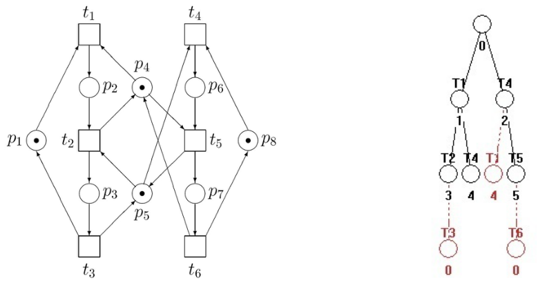
Figure 2.
The united structure of the original Petri-net model with the synthesized supervisor in red (on the left) and its reachability tree showing that there is no deadlock in the controlled (supervised) system (on the right).
Figure 2.
The united structure of the original Petri-net model with the synthesized supervisor in red (on the left) and its reachability tree showing that there is no deadlock in the controlled (supervised) system (on the right).
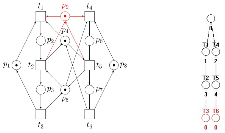
Figure 3.
On the left there is the model of a simple manufacturing system where two processes share two resources. There are several double interconnections between processes and resources. On the right there is the RT of the model with deadlock represented by the node 4 ().
Figure 3.
On the left there is the model of a simple manufacturing system where two processes share two resources. There are several double interconnections between processes and resources. On the right there is the RT of the model with deadlock represented by the node 4 ().
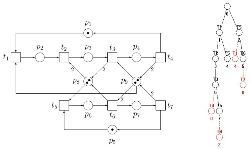
Figure 4.
On the left there is the supervised system (the supervisor is in red) while on the right there is its RT documenting that the system has no deadlocks.
Figure 4.
On the left there is the supervised system (the supervisor is in red) while on the right there is its RT documenting that the system has no deadlocks.
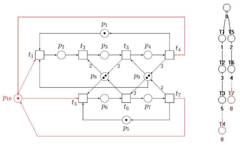
Figure 5.
The RT of the supervised system without deadlocks when in Figure 4 we put and .
Figure 5.
The RT of the supervised system without deadlocks when in Figure 4 we put and .

Figure 6.
On the left there is the supervised system (the supervisor is in red) while on the right there is its RT documenting that the system has no deadlocks.
Figure 6.
On the left there is the supervised system (the supervisor is in red) while on the right there is its RT documenting that the system has no deadlocks.
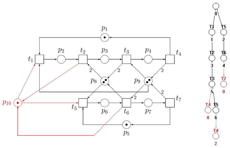
Figure 7.
The RT of the supervised system without deadlocks when in Figure 6 we put and .
Figure 7.
The RT of the supervised system without deadlocks when in Figure 6 we put and .

Figure 8.
On the left there is the GS3PR PN model while on the right there is its RT pointing to the deadlock - the RT node .
Figure 8.
On the left there is the GS3PR PN model while on the right there is its RT pointing to the deadlock - the RT node .
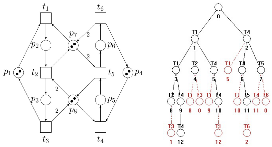
Figure 9.
On the left there is the supervised GS3PR PN model. The supervisor represented by is depicted in red. The RT of the supervised model pointing to its deadlock-freeness is right.
Figure 9.
On the left there is the supervised GS3PR PN model. The supervisor represented by is depicted in red. The RT of the supervised model pointing to its deadlock-freeness is right.
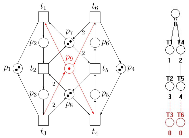
Figure 10.
On the left there is the supervised GS3PR while on the right there is its RT pointing to its deadlock-freeness. The supervisor represented by is depicted in red.
Figure 10.
On the left there is the supervised GS3PR while on the right there is its RT pointing to its deadlock-freeness. The supervisor represented by is depicted in red.
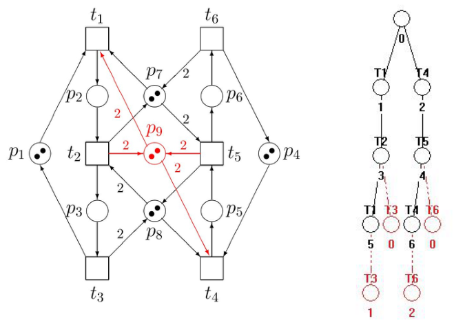
Figure 11.
The uncontrolled S3PR model with minimal resources.
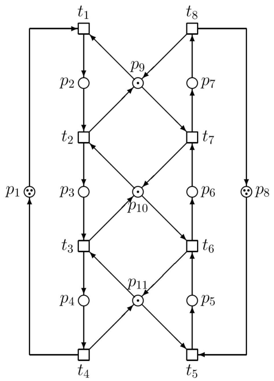
Figure 12.
Transpose of the incidence matrix in the form of a table
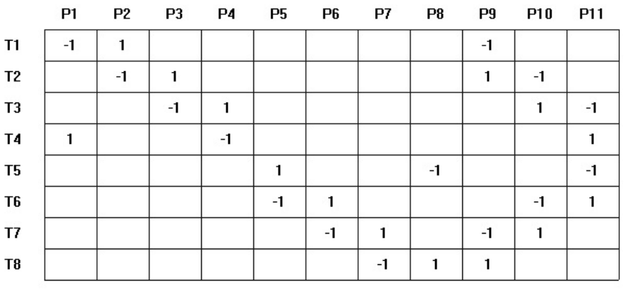
Figure 13.
The RT of the original (uncontrolled) S3PR PN model.
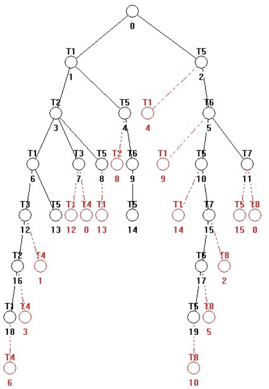
Figure 14.
Supervised S3PR PN model. The supervisor represented by is in red.
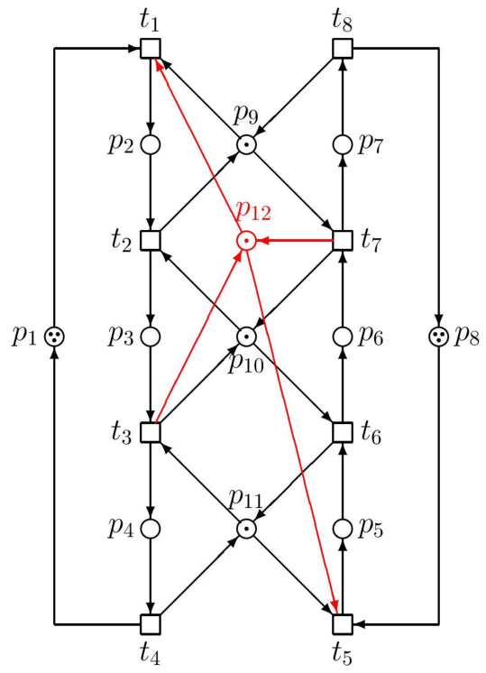
Figure 15.
RT of the supervised S3PR PN model.
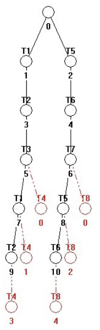
Figure 16.
Supervisor (left) and RT (right) achieved in [4] by means of elementary siphons
Figure 16.
Supervisor (left) and RT (right) achieved in [4] by means of elementary siphons
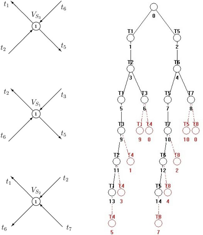
Figure 17.
GS3PR PN model of AMS based on the generalized PN.
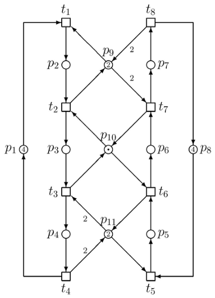
Figure 18.
The supervisor (left) synthesized for the PN model displayed in Figure 17 and the RT of the controlled system.
Figure 18.
The supervisor (left) synthesized for the PN model displayed in Figure 17 and the RT of the controlled system.
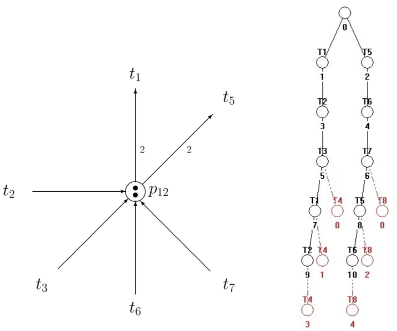
Figure 19.
The simple S4PR GPN model (left) and the transpose of its incidence matrix (right).
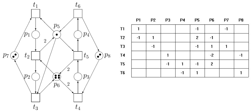
Figure 20.
Simple S4PR PN model supervised by the supervisor in red (up) and its RT documenting deadlock-freeness (down).
Figure 20.
Simple S4PR PN model supervised by the supervisor in red (up) and its RT documenting deadlock-freeness (down).
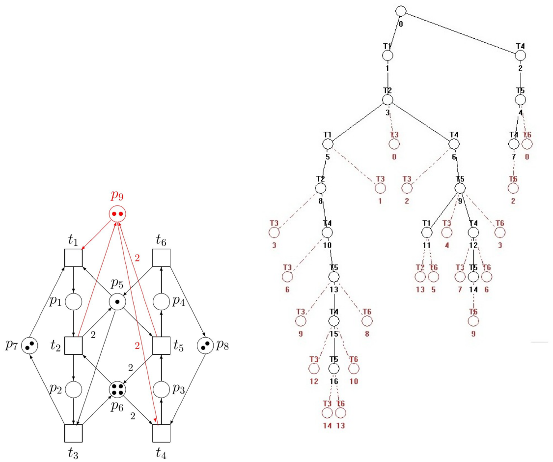
Figure 21.
The original S4PR PN model (on the left) and its RT (on the right).
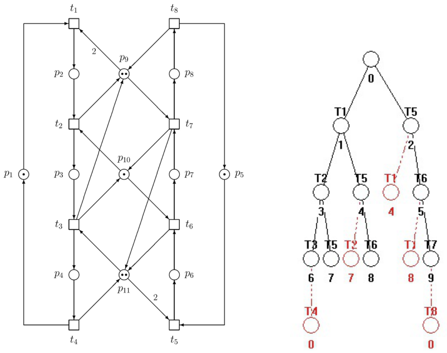
Figure 22.
The supervised S4PR PN model (on the left) and its RT (on the right).
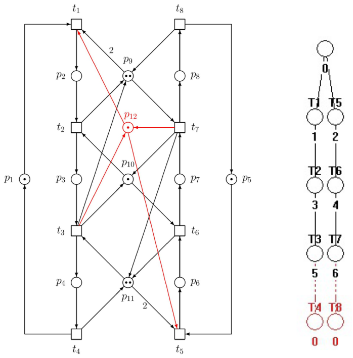
Figure 23.
The S4PR PN model (on the left) and its RT indicant 2 deadlocks (on the right).
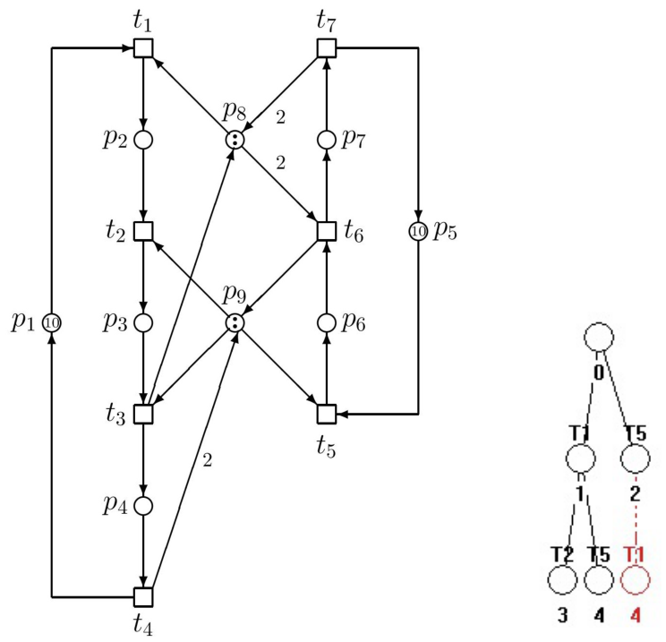
Figure 24.
The incidence matrix of the S4PR PN model.
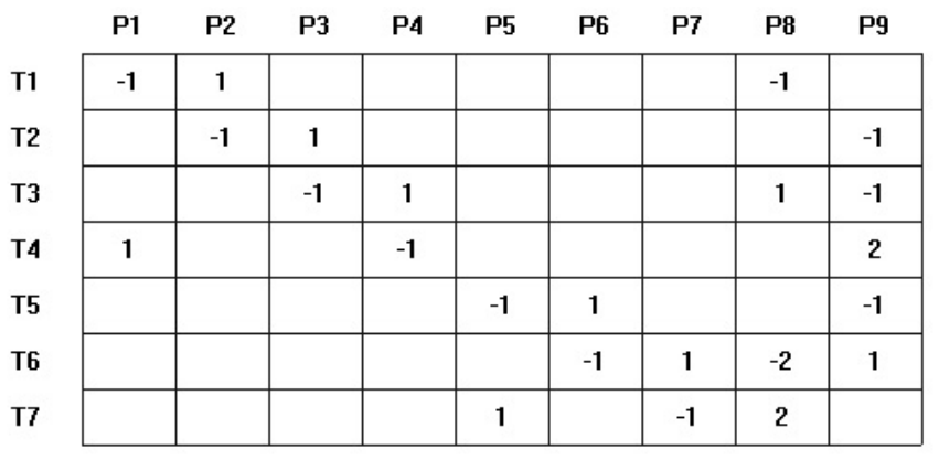
Figure 25.
The controlled S4PR PN model with the supervisor in red (on the left) and its RT documenting its deadlock-freeness (on the right).
Figure 25.
The controlled S4PR PN model with the supervisor in red (on the left) and its RT documenting its deadlock-freeness (on the right).
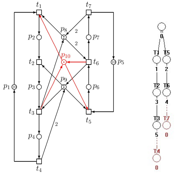
Figure 26.
The GS3PR PN model.
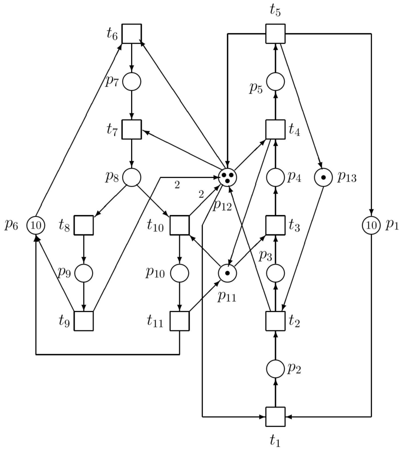
Figure 27.
The incidence matrix of the GS3PR PN model.
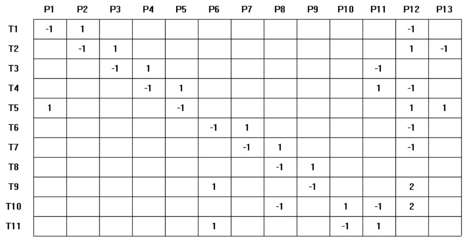
Figure 28.
The supervisor insuring the deadlock-freeness for the S4PR PN model.
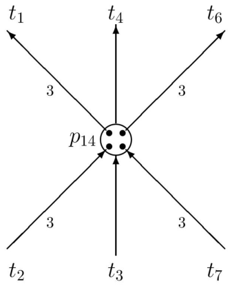
Figure 29.
Another S4PR PN model.
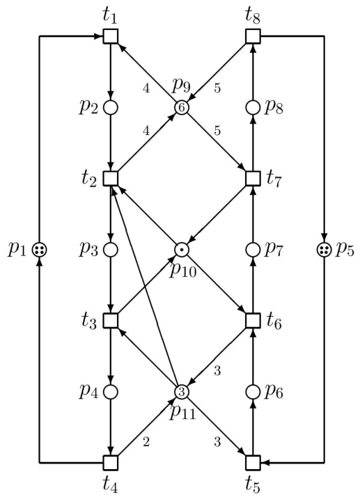
Figure 30.
RT of the S4PR PN model.
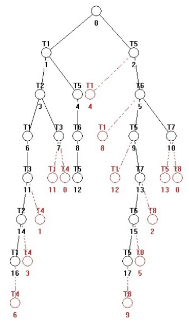
Figure 31.
Supervised S4PR PN model by the supervisor in red (left) and its RT documenting deadlock-freeness.
Figure 31.
Supervised S4PR PN model by the supervisor in red (left) and its RT documenting deadlock-freeness.
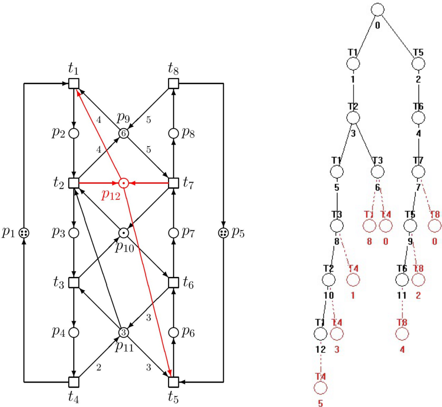
Figure 32.
The large-scale S3PR PN model.
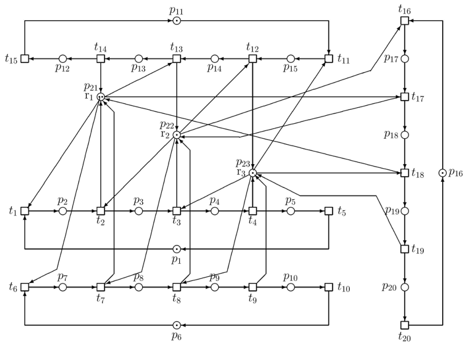
Figure 33.
The supervisor synthesized for the deadlock prevention in the large-scale S3PR PN model.
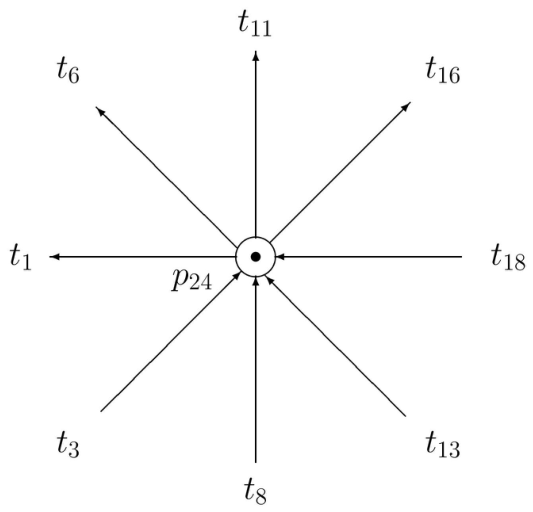
Figure 34.
The S4PR PN model of AMS.
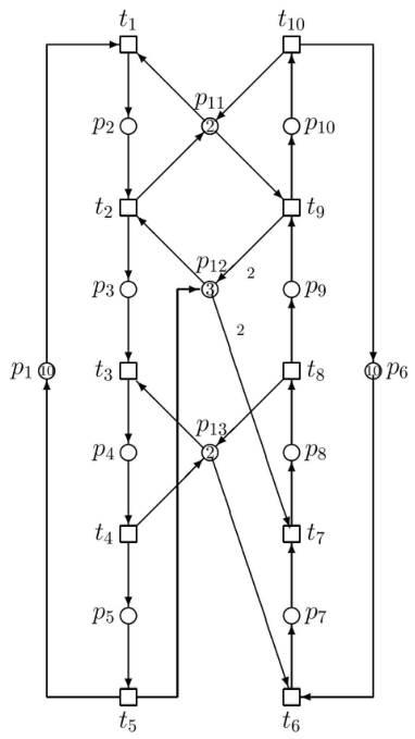
Figure 35.
The supervisor synthesized for the S4PR PN model.
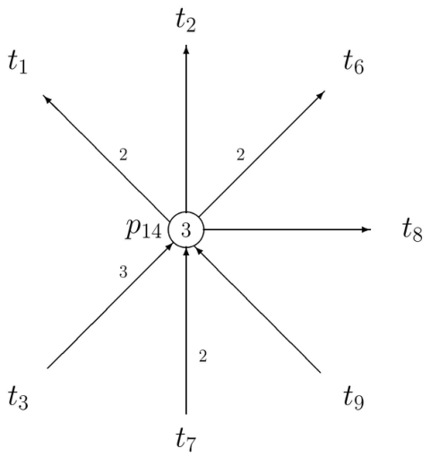
Figure 36.
The S4PR PN model of AMS.
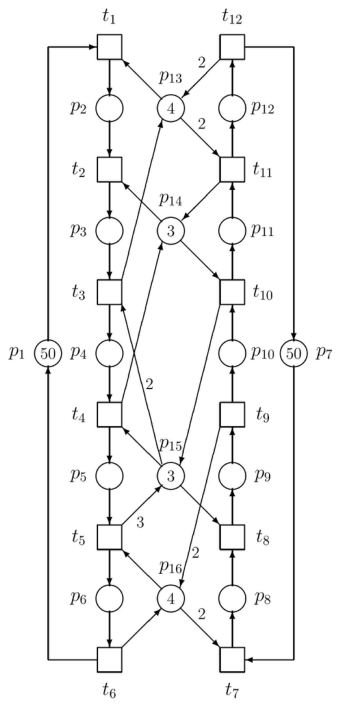
Figure 37.
The supervisor synthesized for the S4PR PN model.
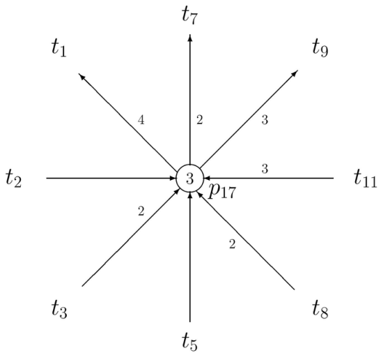
Figure 38.
Two supervisors synthesized for the S4PR PN model.
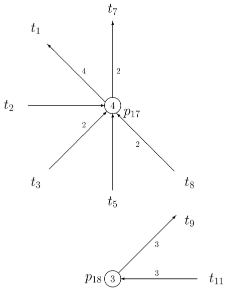
Figure 39.
Large-scale S4PR PN model.
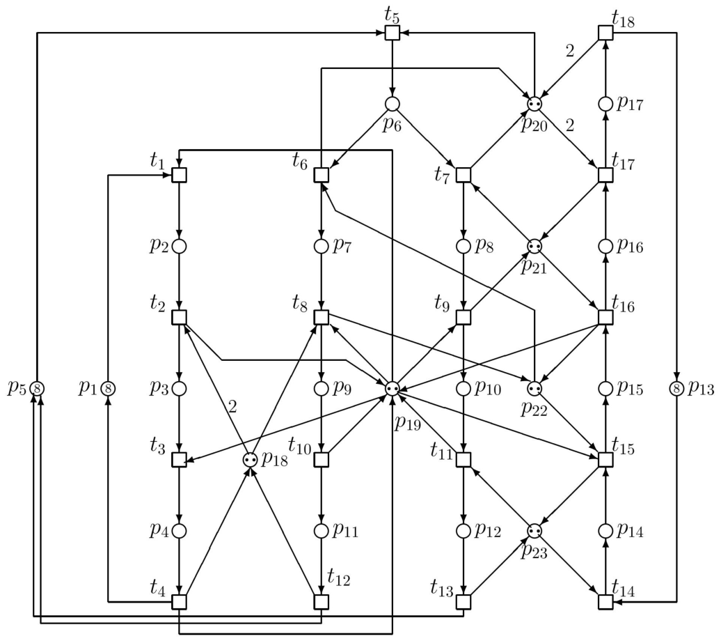
Figure 40.
Transpose of the incidence matrix of that S4PR PN model.
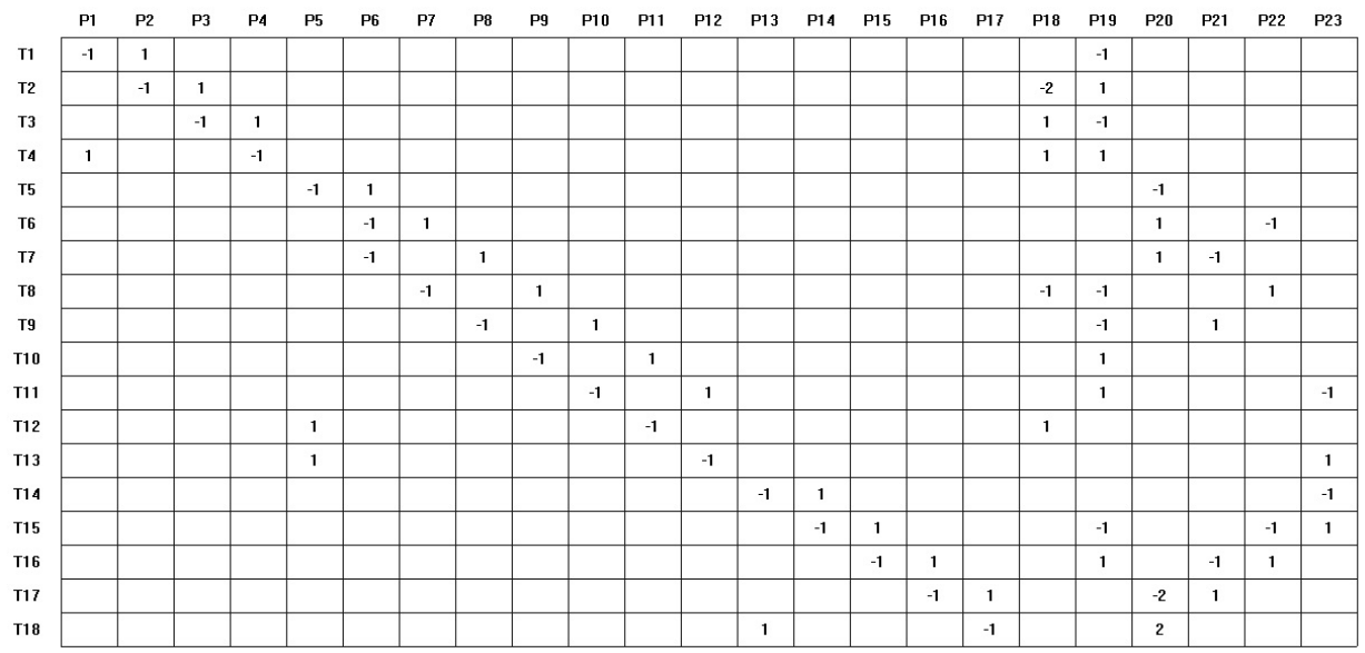
Figure 41.
Supervisor for the large-scale S4PR PN model.
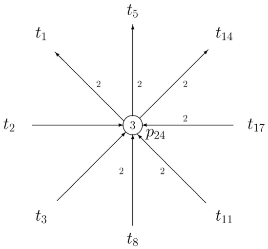

Table 1.
List of deadlocks
Table 2.
Subsets of activity places
Disclaimer/Publisher’s Note: The statements, opinions and data contained in all publications are solely those of the individual author(s) and contributor(s) and not of MDPI and/or the editor(s). MDPI and/or the editor(s) disclaim responsibility for any injury to people or property resulting from any ideas, methods, instructions or products referred to in the content. |
© 2026 by the authors. Licensee MDPI, Basel, Switzerland. This article is an open access article distributed under the terms and conditions of the Creative Commons Attribution (CC BY) license (http://creativecommons.org/licenses/by/4.0/).
Copyright: This open access article is published under a Creative Commons CC BY 4.0 license, which permit the free download, distribution, and reuse, provided that the author and preprint are cited in any reuse.