

Submitted:
04 September 2026
Posted:
04 September 2026
You are already at the latest version
Abstract
High-precision state of charge (SOC) estimation is essential to the reliability, stability, and efficiency of supercapacitor (SC) energy storage systems. However, in practical applications, voltage/current sensors inevitably suffer from irregular noise and bias errors, which weaken the accuracy and robustness of traditional filtering methods. To improve SOC estimation accuracy, a SOC estimation strategy for SCs using estimated value correction (EVC) is proposed. First, the state-space equations are derived from a second-order RC model, and forgetting factor recursive least squares (FFRLS) is used to update parameters, combined with the extended Kalman filter (EKF) to estimate SOC. Second, Sage-Husa adaptive noise mechanism is integrated into the FFRLS-EKF framework to suppress irregular noise. To mitigate sensor bias errors, ampere-hour integration (AHI) results are used to construct a reference value for calibrating the filter output. Finally, experiments under multiple cycling test conditions demonstrate that the proposed correction strategy further suppresses deviation when irregular noise and bias coexist. The proposed EVC-SHEKF framework significantly improves the robustness of SOC estimation under sensor bias and measurement noise conditions, providing a practical solution for reliable state estimation in SC energy storage systems.
Keywords:
supercapacitor
; state estimation
; sensor error
; estimated value correction
; Kalman filter
1. Introduction
Supercapacitors (SCs), characterized by rapid power delivery, strong temperature adaptability, and excellent durability, have been extensively applied across various applications including electric vehicles, new energy power, as well as rail transit [1]. To satisfy high-power requirements, SC cells are commonly assembled in series-parallel configurations to construct energy storage systems. [2]. In these systems, the SC management system (SCMS) is used for managing status of SCs, ensuring system safety and reliability. State of charge (SOC) is a key indicator for the SCMS, which is fundamental to indicating the remaining usable energy and optimizing control strategies. Therefore, high-precision SOC estimation plays an important role in maintaining reliable system operation and enhancing the energy utilization performance of energy storage systems [3].
At present, SOC estimation methods for SCs can be classified into model-free and model-based categories [4]. The former mainly consist of direct calculation and data-driven techniques. Direct calculation methods primarily include ampere-hour integration (AHI) and the open-circuit voltage (OCV) method, both of which are typically open-loop estimation approaches. AHI determines the SOC through time integration of the current, but its inability to correct accumulated deviations makes it sensitive to sensor noise and initial settings [5]. The OCV method estimates state using the pre-established static mapping between OCV and SOC, but it cannot capture the nonlinear dynamics of SCs under complex operating conditions and usually requires long rest periods, which limits its real-time applicability [6]. Consequently, both methods exhibit poor robustness as they lack a feedback mechanism to suppress errors. In contrast, data-driven methods, represented by support vector machine and convolutional neural networks model and predict the SOC of SCs by using a large amount of historical data, making up for the deficiencies of direct computational methods [7,8]. However, their poor generalization under unseen conditions may lead to unstable estimation results [9]. Model-based methods mainly include Luenberger observers, sliding mode observers, and Kalman filters (KF) [10,11,12]. Among these methods, KF and its variants have been extensively studied [13]. KF is based on the assumption of system linearity, and in the case of strong nonlinearity in reality, it will lead to a decrease in estimation accuracy. Meanwhile, the estimation accuracy of KF is also jointly affected by factors such as algorithm precision, system noise, model accuracy and sampling error. To enhance the applicability and estimation performance of KF in complex operating environments, scholars have proposed a variety of improved KF methods [14].
In order to improve the algorithm accuracy and solve the nonlinear problem of the system, algorithms such as extended KF (EKF), unscented KF (UKF) and fading KF (FKF) have been proposed. Among them, UKF has the highest SOC estimation accuracy, and FKF achieves the fastest convergence speed [15,16]. However, these algorithms can only handle system noise modeled as zero-mean Gaussian white noise and cannot handle irregular noise. Therefore, adaptive algorithms were developed to mitigate the effects of irregular noise [17,18,19]. References [20,21] respectively verified the effectiveness of adaptive EKF and adaptive UKF in suppressing irregular noise. Furthermore, all the above-mentioned models assume that the model parameters are accurate. However, in actual situations, the parameters of SCs may change due to temperature and aging. To address the issue of model mismatch, references [22,23] proposed online parameter identification methods that combine EKF and UKF with forgetting factor recursive least squares (FFRLS). Similarly, dual EKF (DEKF) has been employed to concurrently estimate SOC and update parameters by employing two concurrent filters. The dual-structure approach effectively handles the coupling between state variables and time-varying parameters. By dynamically adjusting the model parameters, the impact of parameter variations and model mismatch on the accuracy of SOC estimation has been mitigated.
In practical applications, measurement errors are inevitably introduced by sensors due to bias, drift, and faults, which are often more significant than process noise. These errors generally consist of two distinct components: random noise, which disrupts the statistical characteristics of the data, and systematic bias, which causes a persistent bias in the observation equations [24]. To address these issues, conventional methods including KF and least squares can mitigate disturbances by adjusting algorithm parameters. However, due to the inherent contradiction between bias and variance, parameter optimization cannot take into account both aspects simultaneously [25]. While parameter optimization can suppress random noise, it cannot simultaneously eliminate the systematic bias. The inadequacy of simple parameter adjustment is further explained by the nature of sensor physics. As pointed out in reference [26], certain inherent bias terms are independent of algorithm parameters and are instead coupled with physical characteristics, such as the OCV slope. Because these errors stem from the physical coupling of the sensor, they cannot be eliminated through algorithm optimization alone. This is particularly problematic in scenarios involving sensor damage or extreme sampling errors. Recognizing that parameter tuning is insufficient, researchers have turned to structural modifications and compensation mechanisms. For example, Reference [27] constructed a multi-working state model and designed a switching observer to achieve stable SOC tracking by utilizing the observer structure itself to suppress errors; Reference [28] incorporated current bias directly into the estimation framework and combined it with a PI observation structure to suppress bias interference.
Despite these advancements, most studies focus on reducing error results at the output level, and there remains a lack of quantitative analysis regarding the errors themselves. This gap necessitates the development of online correction mechanisms to ensure high-precision estimation.
To overcome these drawbacks, a state estimation algorithm combining Sage-Husa adaptive EKF (SHEKF) and FFRLS is proposed based on online correction of estimated values. The main contributions of this study are as follows:
(1) An analysis is conducted on the effects of measurement errors on SOC estimation, as well as on the correlation between these errors and the OCV slope.
(2) An online estimated-value correction strategy is developed by combining an AHI-based reference with an OCV slope-weighted compensation mechanism, enabling effective suppression of bias that cannot be eliminated by parameter optimization alone.
(3) A Sage-Husa adaptive noise mechanism is incorporated into the estimation framework to improve robustness under irregular noise.
(4) Experimental validation under DST and UDDS conditions demonstrates that the developed method consistently enhances estimation precision and robustness under coupled voltage/current sensor biases.
The structure of this paper is organized as follows: Section 2 describes the SC models and analyzes the impact of sensor errors and noise on SOC estimation. Section 3 presents the working principle of the developed method. Section 4 presents the platform setup and testing procedures. Section 5 performs the verification and analyzes the results. Section 6 summarizes conclusions.
2. SC Modeling and Error Analysis
2.1. Equivalent Circuit Model of the SC
SCs exhibit internal phenomena such as polarization and relaxation effects. To describe their dynamic characteristics, equivalent circuit models (ECMs) are commonly employed. ECMs can be further categorized into fractional-order models, multi-branch models, and RC network models [29]. The second-order RC ECM achieves a good balance of modeling accuracy and computational complexity, as illustrated in Figure 1.
Where denotes the OCV; is the terminal voltage; denotes the equivalent capacitance; represents the equivalent series resistance; , and , represent the resistance and capacitance of the two RC branches, and denotes the discharge current.
Based on Kirchhoff’s laws, the voltage relationship of the ECM is given by:
SOC is defined as the ratio of the remaining available capacity to the total capacity. Based on the AHI method, SOC can be calculated by integrating the current over time, and its expression is given by:
where represents the Coulombic efficiency, typically set to 1; denotes the rated capacity.
By combining the voltage-current relationship of the ECM with the definition of SOC, the state-space equations can be expressed as:
where represents SOC at time step k; represents the OCV at time step k; and respectively represent process and observation noise.
OCV can be expressed as a polynomial function of SOC:
2.2. Analysis of SOC Estimation Errors
Under real conditions, the measurement value contains ideal value and error:
where and denote the measured terminal voltage and current, respectively; and denote their corresponding true values; and and represent the voltage and current sensor biases.
To facilitate subsequent analysis, the OCV-SOC relationship is locally linearized:
where denotes the local slope of the OCV-SOC curve evaluated at .
The output equation that contains measurement errors can be expressed as follows:
Since this study employs the EKF and its improved variants, the subsequent analysis of error propagation is based on the general EKF update structure [30]. The SOC update equation derived from the first component of the EKF state-update equation:
where denotes the SOC-related element of the Kalman gain vector, i.e., the first element corresponding to the SOC state, and indicates the a priori predicted predicted value of SOC.
The a priori SOC prediction is given by:
The corresponding a priori voltage prediction:
The SOC estimation error:
where denotes the reference SOC and denotes the posterior SOC estimate.
For analytical simplicity, the direct contribution of current sensor bias to the voltage innovation through the ohmic resistance is neglected, while its accumulated effect through SOC prediction is retained. Combining equation (10)-(13), it can be derived that:
The expectation of the estimation error can be expressed in the following recursive form:
where
where denotes the initial estimation error; and denote the cumulative impact of process and measurement noise, respectively; and denote the steady-state deviations induced by the voltage and current measurement bias.
When the system satisfies the stability condition, , the contribution of the initial estimation error asymptotically vanishes:
Under the standard zero-mean noise assumption, and. Therefore, within the adopted local linearized error model, the process and measurement noise do not introduce systematic bias into the mean SOC estimation error:
In practical applications, sensors may encounter irregular noise with a non-zero mean. In such cases, and may no longer be zero, and the corresponding terms in Eqs. (17) and (18) can introduce persistent bias into the mean estimation error. To suppress the effects of irregular noise, it is necessary to employ adaptive algorithms or noise-correlation compensation methods.
While the effects of irregular noise can be mitigated by adaptive methods, steady-state deviations caused by the sensor biases cannot be eliminated by the algorithm itself and require the adoption of auxiliary methods to suppress their impact. For the following steady-state analysis, a local SOC interval is considered in which the OCV-SOC slope varies slowly and can be approximated as a constant. After filter convergence, the SOC-related Kalman gain is also assumed to approach a constant value. Therefore, , . The steady-state deviations are given by:
As shown in the derived formulas, the steady-state SOC error induced by voltage bias is inversely proportional to . As indicated by Eqs. (25) and (26), the voltage-bias-induced error is directly related to the inverse of the local OCV-SOC slope, whereas the contribution of current bias additionally depends on the sampling interval, nominal capacity, and Kalman gain. Therefore, the relative influence of the two sensor biases depends on the specific operating conditions and system parameters. Under the bias amplitudes and test duration considered in this study, the voltage-bias-induced error is more pronounced, as will be further verified experimentally. Therefore, the subsequent discussion focuses primarily on suppressing the steady-state deviation caused by voltage measurement bias.
Similarly, when the stability condition, , is satisfied and the time horizon is sufficiently long, the geometric term vanishes, the steady-state mean estimation error is obtained as:
Theoretical analysis indicates that sensor-induced errors lead to inherent steady-state bias in SOC estimation, which cannot be eliminated solely through parameter optimization, such as tuning the Kalman gain. Furthermore, qualitative analysis reveals that voltage errors exert a more significant impact on estimation accuracy than current errors. Specifically, under voltage-bias-dominant conditions, the magnitude of the steady-state SOC estimation error is inversely related to the magnitude of the local OCV-SOC slope.
3. State Estimation Algorithm
To improve the accuracy of SOC estimation, the Sage-Husa noise adaptive mechanism is first integrated into EKF, so that irregular noise can be suppressed. Secondly, by introducing an AHI reference correction mechanism based on voltage slope weighting, it fundamentally compensates for the inherent deviation caused by sensor errors. The flowchart of the SOC estimation algorithm proposed in this paper is shown in Figure 2.
3.1. FFRLS-EKF Algorithm
3.1.1. Parameter Identification Using FFRLS
To account for the time-varying characteristics of SCs and minimize the impact of model uncertainties, an online parameter identification method is employed. Among various candidates, the FFRLS algorithm is selected because of its superior balance between computational efficiency and identification accuracy. By incorporating a forgetting factor , the algorithm can effectively suppress the influence of historical data and prioritize recent measurements, thereby enhancing its ability to track parameter fluctuations caused by aging or temperature changes. The specific mapping relationship between the parameters of ECM and FFRLS observation vector has been rigorously derived in literature [31,32,33].
The iterative calculation process is detailed as follows:
- Gain vector calculation
- 2.
- Output error computation
where denotes the system output, corresponding to the voltage and current of the SC ECM, represents the output error, denotes the parameter vector.
- 3.
- Parameter update
- 4.
- Covariance matrix update
3.1.2. EKF-Based State Estimation
Time update
- A Priori state estimate:
- 2.
- A Priori covariance:
Measurement update
- Kalman gain:
- 2.
- Posteriori state:
- 3.
- Posteriori covariance:
where and represent the prior state estimate and the corresponding covariance, and denote the posterior estimates, and denote the covariance of the process noise and that of the measurement noise, respectively. denotes the sampled voltage.
3.2. Sage-Husa Noise Adaptive Mechanism
To enhance robustness under non-Gaussian and irregular noise conditions, SHEKF is incorporated to adaptively improve the noise adaptability of the algorithm. The Sage-Husa method dynamically estimates the characteristics of noise, thereby optimizing the noise model and enhancing estimation accuracy for systems with unknown or time-varying noise characteristics. The Sage-Husa formulation yields the following equations for updating noise parameters:
where is the forgetting factor, which controls the weighting of new data. A larger value of assigns greater importance to recent measurements and is suitable for rapidly changing systems, while a smaller value favors more stable systems. Typically, is selected within 0.95-0.99. denotes the innovation sequence, and represent the estimated means of process and measurement noise, respectively.
3.3. Estimated Value Correction (EVC) Based on OCV-SOC Slope
While adaptive filtering methods can mitigate the impact of irregular noise to some extent, it remains inherently limited. Specifically, state estimation based on the EKF is highly reliant on voltage measurements. Based on the aforementioned analysis, any constant sensor bias or voltage measurement error will lead to persistent estimation biases that the algorithm cannot eliminate on its own.
Therefore, an estimated value correction strategy is proposed by utilizing the AHI method as an online reference. The core of this strategy lies in the complementarity of the two methods: the filters are excellent at tracking dynamic system changes but highly sensitive to voltage measurement bias; the AHI method provides a smooth SOC trend because it is entirely independent of voltage measurements. By initializing both the filter and the AHI with the same accurate SOC, derived from OCV-based estimation or recorded data, the AHI result can be used as an auxiliary variable to indirectly reconstruct the reference needed by filter.
Figure 3 presents the procedure used to obtain the correction values.
Figure 3 schematically illustrates the relationship among the reference SOC, the AHI estimate, and the filter estimate; it is used to explain the construction of the correction discrepancy rather than represent a specific experimental trajectory.
Since the true SOC is unavailable during online estimation, the filter error cannot be obtained directly from an exact reference. Therefore, the reference required for filter error estimation is constructed indirectly with the aid of the AHI result. The core idea is to use the available filter estimate and AHI result to indirectly infer the filter error. The difference between the filter estimate and the AHI result at each time step k:
where denotes value from the AHI, denotes the estimation results of the filters. The discrepancy is directly available during online estimation and does not require knowledge of the true SOC.
This difference represents a combination of the filter’s deviation from the true SOC and the AHI’s own integration drift:
where and represent the estimation deviations of the AHI and EKF methods respectively.
Based on the reconstructed filter error, a correction factor γ is introduced to adjust the correction amount, and the corrected SOC is obtained as:
where is the correction gain used to regulate the contribution of the discrepancy signal.
The final corrected SOC is fed back into the filter’s state vector. This feedback mechanism initializes the subsequent state prediction with a corrected value, effectively suppressing the filter’s tendency to deviate due to sensor bias and ensuring a smooth, convergent estimation.
According to the error propagation analysis in Section 2.2, when voltage bias dominates the steady-state estimation error, the magnitude of the SOC bias is approximately inversely related to the magnitude of the local OCV-SOC slope, as expressed in Eq. (28). This relationship provides a physics-based basis for determining the relative correction strength. Therefore, the correction gain is modulated according to the local OCV-SOC slope as follows:
where denotes the local OCV-SOC slope at time step k, denotes the average slope over the considered SOC interval, and is the nominal correction gain. The ratio is dimensionless and preserves the inverse relationship between voltage-bias sensitivity and the local OCV-SOC slope. Thus, a smaller local slope results in a relatively larger correction gain.
For the SC module investigated in this study, the experimentally identified OCV-SOC characteristic is nearly linear, and the variation of over the operating SOC range is limited. Consequently, the slope-dependent modulation of is also small. A nominal gain of ( =0.021) is adopted in this study. The slope weighting therefore serves primarily as a physics-informed modulation of the EVC gain rather than introducing a large gain variation over the tested SOC range.
4. Experimental Setup and Data Acquisition
4.1. SC Test Platform
An experimental platform is developed for SC characteristic testing and the verification of SOC estimation algorithms. The platform consists of a programmable power supply (IT6005C-80-150), a thermal chamber (Binder MK 53), a SC module to be tested, and a host computer for data acquisition and control. The programmable power supply executes precision charging/discharging profiles, while the thermal chamber maintains a stable temperature environment to ensure the consistency of experimental conditions. The upper computer serves as the control hub, synchronized with the power supply to perform real-time data acquisition of voltage, current, and temperature. Figure 4 represents the physical configuration of the experimental arrangement. The SC module selected for this study is the BMOD0165 P048 C0B, and its key parameters are summarized in Table 1.
Since this study focuses on the effects of measurement errors, the nominal capacity is assumed to be accurate. Accordingly, capacity test and OCV characterization were performed prior to algorithm validation. The overall testing procedure is shown in Figure 5.
4.1.1. Capacity Test
During the initialization stage, the SC was first completely discharged to the lower limit cut-off voltage. After a sufficient rest period, it was charged to the fully charged state in constant current and constant voltage mode, followed by another one-hour rest [34,35]. After completing the initialization step, the SC was discharged at a small constant current to the lower limit cut-off voltage. A one-hour rest was then taken to mitigate the polarization effect. After standing, the SC was further discharged. The discharge-rest process were repeated multiple times until the SC voltage stabilizes within the range close cut-off voltage. Finally, the total capacity of the SC was obtained by summing up the discharge capacities of each step. Under the same conditions, the capacity of the SC was measured three times, and the average value was used as its actual value. The results of the three tests were 53.70 Wh, 53.68 Wh and 53.67 Wh. Consequently, the average value of 53.68 Wh was defined as the actual available capacity for this study.
4.1.2. SOC-OCV Curve Identification
After the initialization of the SC, the SC was discharged at a low current, with 5% SOC reduced in each stage. After each discharge step, the SC was allowed to rest for one hour to measure the OCV and SOC as data points. This cyclic discharge-rest-measurement process continued until the voltage reached the lower cut-off limit [36]. To ensure accuracy, three sets of loop test data were averaged and then fitted using polynomial functions ranging from the first to the eighth order. The results indicated that increasing the fitting order beyond a certain point led to overfitting issues. The root mean square error (RMSE) of the second-order fitting was 0.04, which satisfied the accuracy requirements of the subsequent algorithm. Finally, the second-order fitting was selected, yielding the following fitting result:
4.2. Analysis of SC Measurement Errors
In typical integrated energy storage systems, sampling chips and sensors are commonly used to monitor SC parameters. For voltage acquisition in a 48 V-class SC system, common sampling chips and sensors include the TI INA219, ADS1115, LEM LV 25-P, Analog Devices AD8210, and Vicor VI-J60. For devices that cannot directly withstand or measure the full bus voltage, appropriate front-end signal-conditioning circuits, such as voltage dividers or isolation stages, are required to scale the measured voltage to the allowable input range. Similarly, current detection typically employs devices such as LEM HLSR 50-P, Allegro ACS712, TI INA226, Yokogawa CW10, and Honeywell CSNX25 [37]. Each of these components inevitably introduces inherent measurement errors due to hardware limitations; the specific error profiles for the sensors used here are detailed in Table 2.
5. Experimental Validation and Results Analysis
5.1. SOC Estimation Under Error-Free Conditions
To verify the fundamental state estimation capabilities of the algorithms, experiments were conducted under dynamic stress test (DST) and urban dynamometer driving schedule (UDDS). For all test scenarios, the initial SOC was set to 1, and the temperature was maintained at 25 °C. To ensure a fair comparison, the initial parameters for the algorithms, including the process and measurement noise covariance matrix were individually optimized through empirical tuning to ensure that each algorithm performs at its respective best. The comparative results of the SOC estimation under these error-free conditions are shown in Figure 6. Rows (a)-(c) show the SOC trajectory, terminal voltage, and SOC estimation error, respectively, while row (d) summarizes the statistical metrics, Columns (1) and (2) correspond to the DST and UDDS driving cycles. According to the statistical results shown in Figure 6, under the UDDS condition, the maximum absolute error (MaxAE), mean error (ME), and root mean square error (RMSE) of EKF are 1.87%, 0.31%, and 0.48%, respectively, while the corresponding values of UKF are 1.46%, 0.29%, and 0.41%. For the proposed SHEKF, the MaxAE, ME, and RMSE are 0.63%, 0.08%, and 0.14%, respectively. It can be observed that the SHEKF achieves the smallest MaxAE, ME, and RMSE among the three algorithms. A similar trend can also be observed under the DST condition. These results indicate that the proposed method provides higher SOC estimation accuracy than the EKF and UKF under dynamic operating conditions. In addition, all three algorithms are able to accomplish SOC estimation, which also demonstrates that the SC model is capable of supporting state estimation.
5.2. Sensor Bias Gradient Experiments
To further investigate the influence of coupled sensor biases on estimation stability, coupled bias gradient experiments are conducted across DST and UDDS. The experiments are designed by fixing the voltage bias at three levels: 0.2 V, 0.5 V, and 1 V. while varying the current biases between 0.05 A and 0.1 A. This setup aims to verify the theoretical analysis regarding the algorithms’ sensitivity to different errors and to evaluate the effectiveness of the EVC mechanism. The results under these coupled bias conditions are shown in Figure 7 and Figure 8. For each figure, the subplots are organized as follows: (a-1), (a-2), and (a-3) show the SOC estimating performance under the three voltage-bias conditions, respectively; (b-1), (b-2), and (b-3) show the SOC error fluctuations for the corresponding voltage bias levels. The quantitative performance of the four algorithms are summarized in Table 3 and Table 4.
For the DST condition, the SOC estimation results and corresponding SOC error curves are shown in Figure 7, and the quantitative results are listed in Table 3. As shown in Table 3, under the bias condition of 0.05 A and 0.2 V, the RMSEs of SOC based on EKF, UKF, SHEKF, and EVC-SHEKF are 0.90%, 0.83%, 0.58%, and 0.39%, respectively, while the corresponding MEs are 0.75%, 0.71%, 0.52%, and 0.15%. When the current bias increases from 0.05 A to 0.1 A at the same voltage bias of 0.2 V, the corresponding RMSEs become 0.89%, 0.82%, 0.58%, and 0.39%, respectively, indicating only slight changes. By contrast, when the voltage bias increases from 0.2 V to 0.5 V at a fixed current bias of 0.05 A, the RMSE of EKF increases from 0.90% to 1.46%, while UKF increases from 0.83% to 1.37%. The RMSE of SHEKF also rises from 0.58% to 1.13%, whereas the corresponding RMSE of EVC-SHEKF rises from 0.39% to 0.84%. Similar variation can also be observed in the ME results shown in Table 3. These results indicate that, under the tested bias amplitudes and test duration, the SOC estimation error is more sensitive to voltage bias than to the variation in current bias. Meanwhile, among the four algorithms, EVC-SHEKF consistently achieves the smallest error indices, which demonstrates that the EVC mechanism can effectively suppress estimation deviation under coupled sensor bias conditions.
For the UDDS condition, the SOC estimation results and SOC error curves are shown in Figure 8, and the quantitative results are listed in Table 4. As shown in Table 4, under the bias condition of 0.05 A and 0.2 V, the RMSEs of EKF, UKF, SHEKF, and EVC-SHEKF are 0.85%, 0.84%, 0.61%, and 0.44%, respectively, while the corresponding MEs are 0.76%, 0.73%, 0.51%, and 0.15%. When the current bias increases to 0.1 A while the voltage bias remains 0.2 V, the RMSEs change to 0.84%, 0.84%, 0.61%, and 0.44%, respectively, which shows that under the considered bias amplitudes and test duration, the variation in current bias produces only limited changes, whereas increasing voltage bias causes a more pronounced estimation deterioration. However, when the voltage bias increases from 0.2 V to 1 V at a fixed current bias of 0.05 A, the RMSEs of EKF, UKF, SHEKF, and EVC-SHEKF increase from 0.85%, 0.84%, 0.61%, and 0.44% to 2.42%, 2.38%, 2.14%, and 1.11%, respectively. It can be seen that the UDDS condition presents the same trend as the DST condition, namely that voltage bias causes more severe estimation deterioration than current bias, and the EVC-SHEKF always provides the best estimation performance among the four algorithms. Therefore, the experimental results further verify the previous theoretical analysis and confirm that the proposed EVC mechanism can significantly improve estimation robustness and dynamic response capability under complex operating conditions.
5.3. Applicability of the EVC Strategy to Kalman-Filter-Based Estimators
To evaluate the compatibility of the EVC strategy with different Kalman-filter-based estimators, the correction mechanism is further incorporated into EKF, UKF, and SHEKF. Experiments are conducted under DST and UDDS, with sensor biases introduced to simulate real disturbances. The comprehensive results are shown in Figure 9 (DST) and Figure 10 (UDDS). In each figure, (a-1), (a-2), and (a-3) show the SOC curves for the EKF, UKF, and SHEKF algorithms, respectively. Each plot compares five curves: the reference SOC, the filter output without error, the uncorrected filter output under error, the results of the AHI, and the SOC estimated by the EVC method; (b-1), (b-2), and (b-3) present the quantitative error analysis in terms of MaxAE, ME, and RMSE, respectively.
For the DST condition, the experimental results are shown in Figure 9. After the introduction of the EVC mechanism, the SOC estimation curves of EKF, UKF, and SHEKF all move closer to the reference SOC, and the deviation caused by sensor bias is significantly reduced. After applying the EVC strategy, the RMSE of SHEKF decreases from 2.36% to 0.71%. For the EKF and UKF frameworks, the error indices also decrease from 2.26% to 0.61% and from 2.07% to 0.41%, respectively. It can be observed that the EVC strategy improves the estimation performance in all three filtering frameworks under the DST condition. These results demonstrate that the EVC strategy can be effectively incorporated into the three Kalman-filter-based estimators investigated in this study.
For the UDDS condition, the corresponding results are shown in Figure 10. The corresponding statistical results show a similar trend to those under the DST condition, indicating that the EVC strategy can also effectively reduce the estimation errors of different algorithms under more complex operating conditions. Overall, the above results confirm that the proposed EVC strategy exhibits good compatibility with the tested Kalman-filter-based estimation frameworks.
6. Conclusions
In this work, a SC SOC estimation method based on online correction of estimated values is developed to enhance the estimation accuracy of SCs under sensor errors. First, a second-order RC model is adopted with parameters identified online by FFRLS. Under error-free conditions, the SHEKF algorithm achieves a high-precision baseline with an RMSE within 1%, outperforming conventional EKF and UKF. Second, the sensitivity analysis reveals that while SHEKF excels in noise adaptation, it remains susceptible to voltage sensor errors. Conversely, current sensor bias can lead to accumulated drift in the AHI result. Then, an online estimated value correction strategy is developed. Based on the inverse relationship between voltage-bias-induced SOC error and the local OCV-SOC slope, the EVC strategy uses the AHI estimate as an auxiliary reference and applies a slope-modulated correction gain, further enhancing the accuracy of SOC estimation. Finally, the proposed method is validated across DST and UDDS driving cycles. The experimental results demonstrate that the EVC-SHEKF effectively improves the estimation accuracy and stability. Under the tested DST and UDDS conditions with coupled sensor noise and bias, the EVC-SHEKF consistently reduces the SOC estimation error compared with the uncorrected estimators.
Author Contributions
Conceptualization, H.W., J.D. and K.Z.; methodology, H.W.; software, H.W.; validation, H.W.; formal analysis, H.W. and J.D.; investigation, H.W. and L.W.; resources, J.D. and K.Z.; data curation, H.W., J.D. and L.W.; writing—original draft preparation, H.W. and J.D.; writing—review and editing, H.W.; visualization, H.W. and L.W.; supervision, J.D. and K.Z.; funding acquisition, J.D. All authors have read and agreed to the published version of the manuscript.
Funding
This research was funded by the National Natural Science Foundation of China, grant number 52177211.
Institutional Review Board Statement
Not applicable.
Informed Consent Statement
Not applicable.
Data Availability Statement
The data presented in this study are available on request from the corresponding author.
Conflicts of Interest
The authors declare no conflicts of interest. The funders had no role in the design of the study; in the collection, analyses, or interpretation of data; in the writing of the manuscript; or in the decision to publish the results.
Abbreviations
The following abbreviations are used in this manuscript:
| SOC | state of charge |
| SC | supercapacitor |
| EVC | estimated value correction |
| FFRLS | forgetting factor recursive least squares |
| EKF | extended Kalman filter |
| AHI | ampere-hour integration |
| SCMS | SC management system |
| OCV | open circuit voltage |
| KF | Kalman filter |
| UKF | unscented Kalman filter |
| FKF | fading Kalman filter |
| DEKF | dual extended Kalman filter |
| SHEKF | Sage-Husa adaptive extended Kalman filter |
| ECM | equivalent circuit model |
| DST | dynamic stress test |
| UDDS | urban dynamometer driving schedule |
| MaxAE | maximum absolute error |
| ME | mean error |
| RMSE | root mean square error |
References
- Afshan, M.; Kumar, N.; Das, S.; E.M., H.; Rani, D.; Sharangi, S.; Pahuja, M.; Siddiqui, S.A.; Rani, S.; Chaudhary, N.; et al. Electronic modulation of MOF-engineered bimetallic phosphides for cost-effective ampere-level water splitting and continuous hydrogen production via supercapacitor integration. J. Energy Chem. 2025, 108, 221–238. [CrossRef]
- Zhang, X.; Zhang, Z.; Zhou, Z. MXene-based materials for electrochemical energy storage. J. Energy Chem. 2018, 27, 73–85. [CrossRef]
- Chaluvachar, P.; Sudhakar, Y.N.; Mahesha, G.T.; Nair, V.G.; Desai, N.; Pai, D.K. Emerging role of graphitic carbon nitride in advanced supercapacitors: A comprehensive review. J. Energy Chem. 2025, 103, 498–524. [CrossRef]
- Naseri, F.; Karimi, S.; Farjah, E.; Schaltz, E. Supercapacitor management system: A comprehensive review of modeling, estimation, balancing, and protection techniques. Renew. Sustain. Energy Rev. 2022, 155, 111913. [CrossRef]
- Li, Z.; Chen, C.; Yang, R.; Li, H.; Xiong, R. Entropy-driven online open circuit voltage identification for precise state estimation in lithium-ion batteries. iScience 2025, 28, 113290. [CrossRef]
- Zhang, J.; Liu, W.; Du, M.; Xu, Q.; Hung, M.; Xiang, R.; Liao, M.; Wang, X.; Wang, B.; Yu, A.; et al. Kinetic investigation of the energy storage process in graphene fiber supercapacitors: Unraveling mechanisms, fabrications, property manipulation, and wearable applications. Carbon Energy 2025, 7, e625. [CrossRef]
- Liu, B.; Wang, H.; Tseng, M.-L.; Li, Z. State of charge estimation for lithium-ion batteries based on improved barnacle mating optimizer and support vector machine. J. Energy Storage 2022, 55, 105830. [CrossRef]
- Wang, D.; Chang, Y.; Ji, P.; Suo, Y.; Chen, N. State of charge prediction of mine-used LiFePO₄ battery based on PSO-Catboost. Energies 2024, 17, 5920. [CrossRef]
- Zhang, C.; Wang, T.; Zhang, B.; Qiao, L.; Lian, G.; Wei, M. Closed-loop state of charge estimation of lithium-ion batteries based on machine learning and Kalman filtering. Arab. J. Sci. Eng. 2026, 51, 1651–1668. [CrossRef]
- Rezaei, O.; Dinh, T.Q. A robust adaptive battery state of charge estimation based on integrated Luenberger observer: An investigation for electric urban air mobility application. J. Energy Storage 2025, 128, 117128. [CrossRef]
- Nath, A.; Gupta, R.; Mehta, R.; Bahga, S.S.; Gupta, A.; Bhasin, S. Attractive ellipsoid sliding mode observer design for state of charge estimation of lithium-ion cells. IEEE Trans. Veh. Technol. 2020, 69, 14701–14712. [CrossRef]
- Hu, X.; Sun, F.; Zou, Y. Estimation of state of charge of a lithium-ion battery pack for electric vehicles using an adaptive Luenberger observer. Energies 2010, 3, 1586–1603. [CrossRef]
- Chen, M.; Costa-Castelló, R.; Batlle, C.; Na, J. Metal hydride storage tanks real-time state of charge estimation based on nonlinear observer with a non-observable subsystem. Appl. Energy 2025, 399, 126448. [CrossRef]
- Plett, G.L. Sigma-point Kalman filtering for battery management systems of LiPB-based HEV battery packs: Part 1: Introduction and state estimation. J. Power Sources 2006, 161, 1356–1368. [CrossRef]
- Yang, J.; Xia, B.; Shang, Y.; Huang, W.; Mi, C.C. Adaptive state-of-charge estimation based on a split battery model for electric vehicle applications. IEEE Trans. Veh. Technol. 2017, 66, 10889–10898. [CrossRef]
- Peng, S.; Chen, C.; Shi, H.; Yao, Z. State of charge estimation of battery energy storage systems based on adaptive unscented Kalman filter with a noise statistics estimator. IEEE Access 2017, 5, 13202–13212. [CrossRef]
- Luo, Z.; Qu, D.; Fan, L.; Yang, S. State of charge estimation for the vanadium redox flow battery based on the Sage–Husa adaptive extended Kalman filter. Int. J. Circuit Theory Appl. 2024, 52, 380–395. [CrossRef]
- Gu, C.; Ni, L.; Tian, X.; Fan, C. Physics-based battery SOC estimation: A joint data-driven and window-varying adaptive extended Kalman filter approach. J. Energy Storage 2025, 121, 116465. [CrossRef]
- Du, J.; Wang, J.; Tan, B.; Cao, X.; Qu, C.; Ou, Y.; He, X.; Xiong, L.; Tu, R. Estimation of battery state of charge based on changing window adaptive extended Kalman filtering. J. Energy Storage 2024, 103, 114325. [CrossRef]
- Taborelli, C.; Onori, S. State of charge estimation using extended Kalman filters for battery management system. In Proceedings of the 2014 IEEE International Electric Vehicle Conference (IEVC), Florence, Italy, 17–19 December 2014; pp. 1–8. [CrossRef]
- Meng, J.; Luo, G.; Gao, F. Lithium polymer battery state-of-charge estimation based on adaptive unscented Kalman filter and support vector machine. IEEE Trans. Power Electron. 2016, 31, 2226–2238. [CrossRef]
- Liu, Z.; Chen, S.; Wu, H.; Huang, H.; Zhao, Z. A combined state of charge estimation method for lithium-ion batteries using cubature Kalman filter and least square with gradient correction. Adv. Theory Simul. 2022, 5, 2100331. [CrossRef]
- Li, X.; Zheng, Z.; Meng, J.; Wang, Q. Robust estimation of lithium battery state of charge with random missing current measurement data. Electronics 2024, 13, 4436. [CrossRef]
- Kadem, O.; Kim, J. Mitigation of state of charge estimation error due to noisy current input measurement. Proc. Inst. Mech. Eng. Part I J. Syst. Control Eng. 2024, 238, 34–46. [CrossRef]
- Tong, Y.; Zheng, Z.; Fan, W.; Liu, Z. Improved unscented Kalman filter for state of charge estimation of lithium-ion battery with one-step randomly measurement loss and inaccurate noise covariance matrices. Digit. Signal Process. 2022, 131, 103780. [CrossRef]
- Lin, X. Theoretical analysis of battery SOC estimation errors under sensor bias and variance. IEEE Trans. Ind. Electron. 2018, 65, 7138–7148. [CrossRef]
- Li, H.; Zhou, Z.; Hu, C. A switching observer for state-of-charge estimation of reconfigurable supercapacitors. Appl. Sci. 2024, 14, 8005. [CrossRef]
- Wu, L.; Liu, K.; Pang, H.; Jin, J. Online SOC estimation based on simplified electrochemical model for lithium-ion batteries considering current bias. Energies 2021, 14, 5265. [CrossRef]
- Hu, X.; Li, S.; Peng, H. A comparative study of equivalent circuit models for Li-ion batteries. J. Power Sources 2012, 198, 359–367. [CrossRef]
- Yuan, S.; Wu, H.; Yin, C. State of charge estimation using the extended Kalman filter for battery management systems based on the ARX battery model. Energies 2013, 6, 444–470. [CrossRef]
- Nadeau, A.; Sharma, G.; Soyata, T. State-of-charge estimation for supercapacitors: A Kalman filtering formulation. In Proceedings of the 2014 IEEE International Conference on Acoustics, Speech and Signal Processing (ICASSP), Florence, Italy, 4–9 May 2014; pp. 2194–2198. [CrossRef]
- Sun, X.; Ji, J.; Ren, B.; Xie, C.; Yan, D. Adaptive forgetting factor recursive least square algorithm for online identification of equivalent circuit model parameters of a lithium-ion battery. Energies 2019, 12, 2242. [CrossRef]
- Zhao, X.; Wang, T.; Li, L.; Cheng, Y. Estimation of lithium-ion battery SOC based on IFFRLS-IMMUKF. World Electr. Veh. J. 2024, 15, 494. [CrossRef]
- Yang, T.; Li, J.; Zhan, N.; Wang, X.; Zhang, X. A SOC estimation method for energy storage batteries based on FFRLS-EKF. In Proceedings of the 2025 2nd International Symposium on New Energy Technologies and Power Systems (NETPS 2025), Hangzhou, China, 23–25 May 2025; pp. 298–303. [CrossRef]
- Asghar, M.A.; Ahmad, S.; Alanazi, A.K.; Demir, M.; Mansoor, M.A.; Iqbal, M. Synergistic integration of reduced graphene oxide with Ti₃CN MXene for superior electrochemical energy storage. Mater. Today Commun. 2025, 49, 114273. [CrossRef]
- Sandoval-Chileño, M.A.; Lozada-Castillo, N.; Cortez, R.; Luviano-Juárez, A.; Vazquez-Arenas, J. State of charge estimator based on tractable extended state observers for supercapacitor packs. J. Energy Storage 2024, 85, 111086. [CrossRef]
- Chen, Z.; Yang, L.; Zhao, X.; Wang, Y.; He, Z. Online state of charge estimation of Li-ion battery based on an improved unscented Kalman filter approach. Appl. Math. Model. 2019, 70, 532–544. [CrossRef]
Figure 1.
Second-order RC equivalent circuit model of the SC.
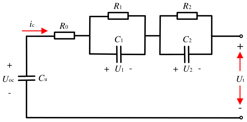
Figure 2.
Flowchart of SOC estimation algorithm.
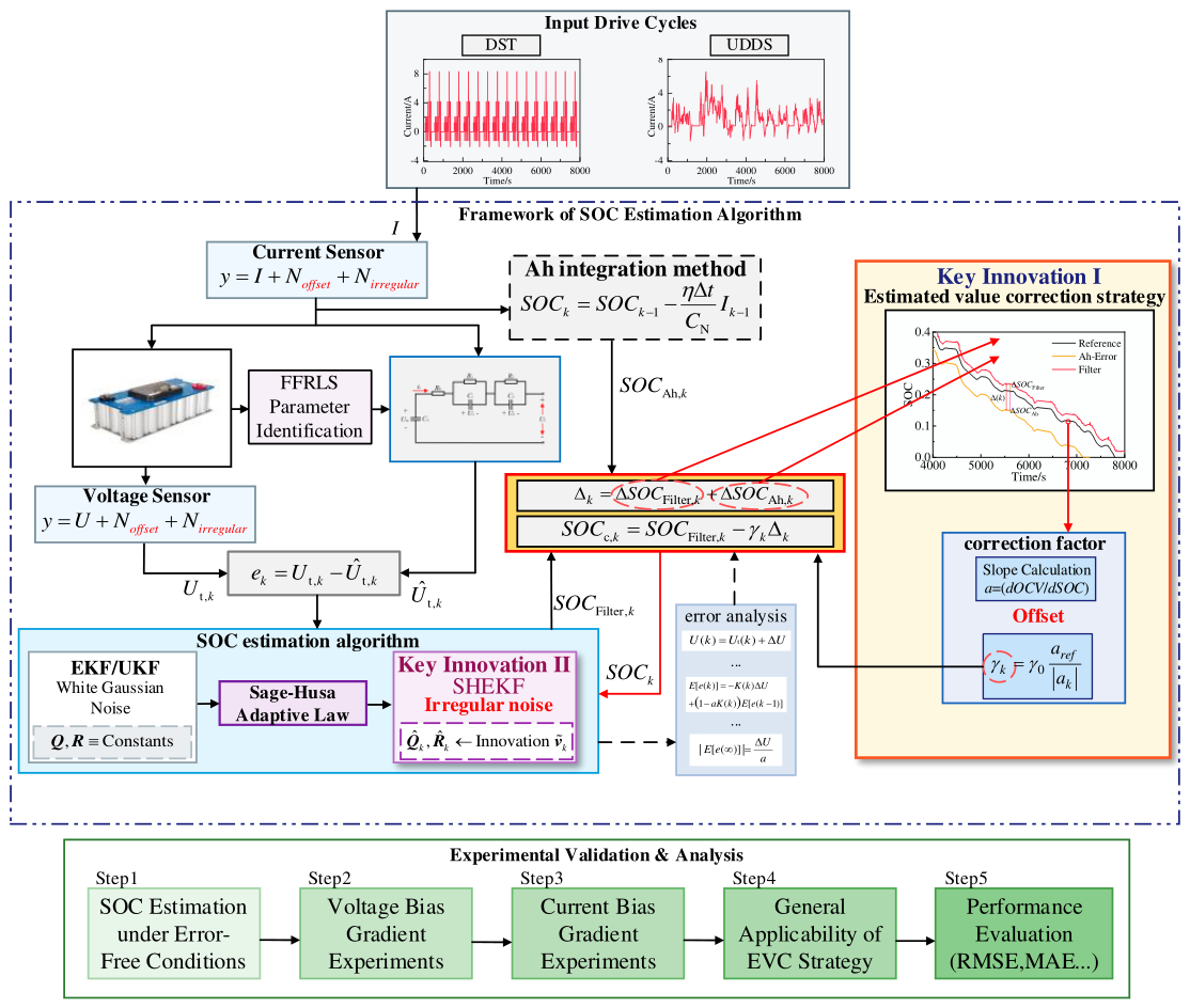
Figure 3.
Construction of the EVC discrepancy signal.
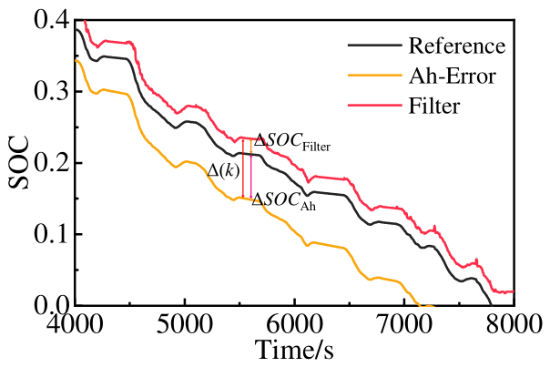
Figure 4.
The experimental test platform.
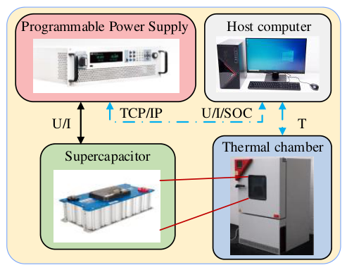
Figure 5.
Flowchart of SC test.
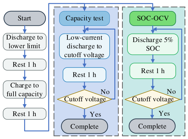
Figure 6.
SOC estimation results under error-free conditions. Rows (a)-(c) present the SOC trajectory, voltage, and SOC estimation error, respectively, while row (d) presents the statistical error metrics (MaxAE, ME, and RMSE). Columns (1) and (2) correspond to the DST and UDDS driving cycles.
Figure 6.
SOC estimation results under error-free conditions. Rows (a)-(c) present the SOC trajectory, voltage, and SOC estimation error, respectively, while row (d) presents the statistical error metrics (MaxAE, ME, and RMSE). Columns (1) and (2) correspond to the DST and UDDS driving cycles.
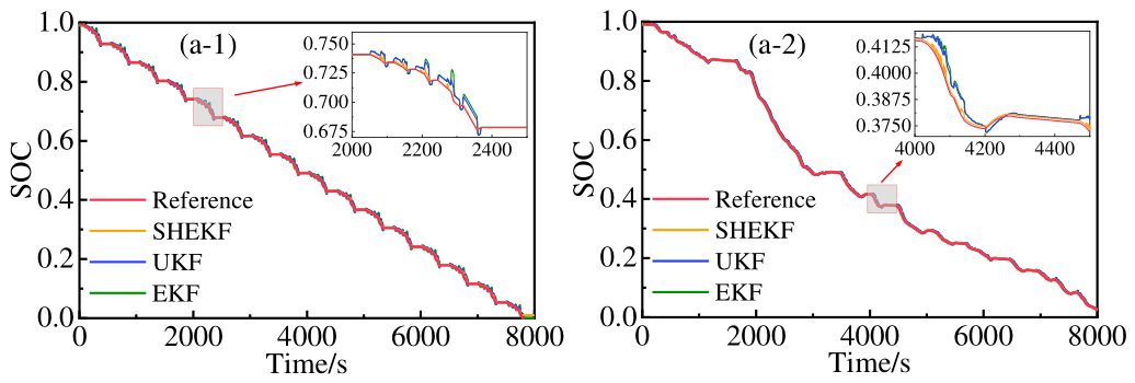
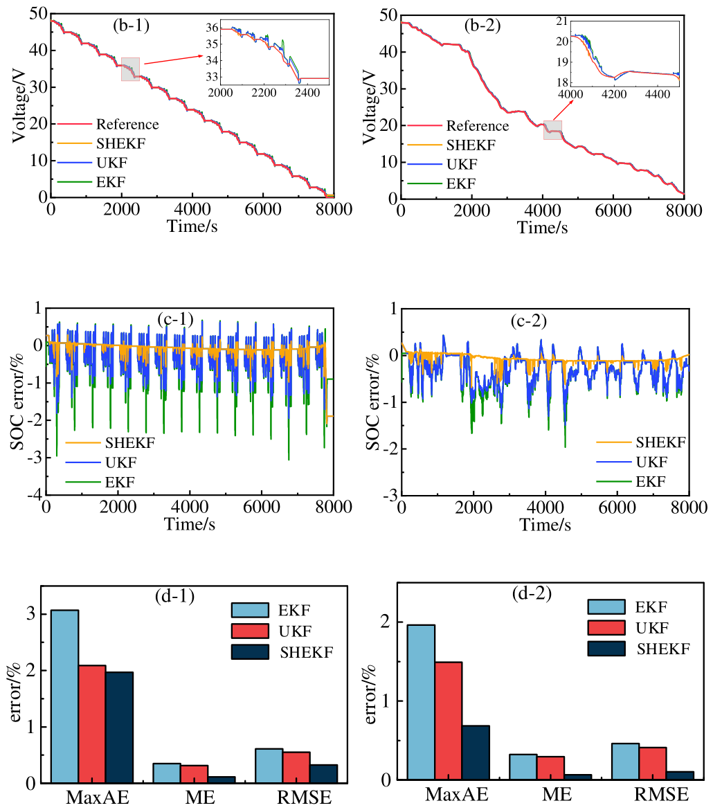
Figure 7.
SOC estimation results under DST condition with bias gradient. Row (a) shows the SOC estimation curves, and row (b) presents the corresponding SOC errors. Columns (1)-(3) correspond to voltage biases of 0.2 V, 0.5 V, and 1 V, respectively.
Figure 7.
SOC estimation results under DST condition with bias gradient. Row (a) shows the SOC estimation curves, and row (b) presents the corresponding SOC errors. Columns (1)-(3) correspond to voltage biases of 0.2 V, 0.5 V, and 1 V, respectively.
Figure 8.
SOC estimation results under UDDS condition with bias gradient. Row (a) shows the SOC estimation curves, and row (b) presents the corresponding SOC errors. Columns (1)-(3) correspond to voltage biases of 0.2 V, 0.5 V, and 1 V, respectively.
Figure 8.
SOC estimation results under UDDS condition with bias gradient. Row (a) shows the SOC estimation curves, and row (b) presents the corresponding SOC errors. Columns (1)-(3) correspond to voltage biases of 0.2 V, 0.5 V, and 1 V, respectively.
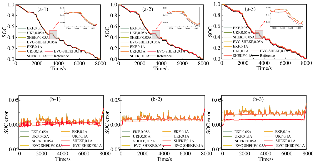
Figure 9.
SOC estimation results of the EVC strategy under DST conditions. Row (a) shows the SOC trajectories from EKF, UKF, and SHEKF, respectively. Row (b) presents the corresponding statistical error metrics, including MaxAE, ME, and RMSE.
Figure 9.
SOC estimation results of the EVC strategy under DST conditions. Row (a) shows the SOC trajectories from EKF, UKF, and SHEKF, respectively. Row (b) presents the corresponding statistical error metrics, including MaxAE, ME, and RMSE.
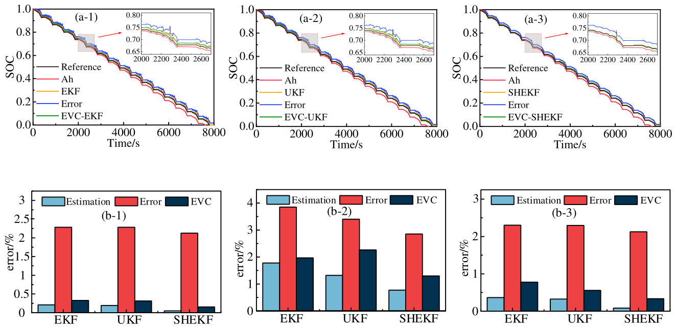
Figure 10.
SOC estimation results of the EVC strategy under UDDS conditions. Row (a) shows the SOC trajectories from EKF, UKF, and SHEKF, respectively. Row (b) presents the corresponding statistical error metrics, including MaxAE, ME, and RMSE.
Figure 10.
SOC estimation results of the EVC strategy under UDDS conditions. Row (a) shows the SOC trajectories from EKF, UKF, and SHEKF, respectively. Row (b) presents the corresponding statistical error metrics, including MaxAE, ME, and RMSE.
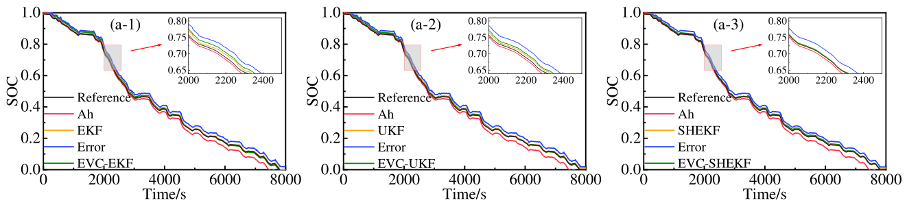
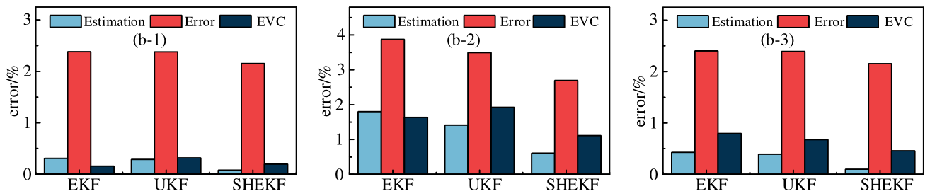

Table 1.
Critical parameters of the SC.
| SC parameter | Specification |
| Rated Capacitance | 165 F |
| Rated Voltage | 48 V |
| Test Current | 100 A |
| Stored Energy | 53 Wh |
Table 2.
Typical measurement errors of the selected voltage and current sensors.
| VoltageSensor | Voltage Error/V | CurrentSensor | Current Error/A |
| TI INA219 | 0.25 | LEM HLSR 50-P | 0.05 |
| LEM LV 25-P | 0.4 | TI INA226 | 0.1 |
| AD8210 | 0.1 | Allegro ACS712 | 0.075 |
| ADS1115 | 0.05 | Yokogawa CW10 | 0.05 |
| Vicor VI-J60 | 0.5 | Honeywell CSNX25 | 0.02 |
Table 3.
Statistical analysis of SOC estimation under DST with different sensor biases.
| Condition | ME (%) | RMSE (%) | ||||||
| EKF | UKF | SHEKF | EVC-SHEKF | EKF | UKF | SHEKF | EVC-SHEKF | |
| DST, 0.05 A, 0.2 V | 0.749 | 0.708 | 0.516 | 0.146 | 0.903 | 0.833 | 0.577 | 0.394 |
| DST, 0.1 A, 0.2 V | 0.735 | 0.695 | 0.515 | 0.142 | 0.891 | 0.823 | 0.576 | 0.392 |
| DST, 0.05 A, 0.5 V | 1.367 | 1.302 | 1.111 | 0.812 | 1.458 | 1.373 | 1.134 | 0.838 |
| DST, 0.1 A, 0.5 V | 1.353 | 1.290 | 1.109 | 0.811 | 1.445 | 1.362 | 1.132 | 0.838 |
| DST, 0.05 A, 1 V | 2.384 | 2.301 | 2.112 | 1.077 | 2.444 | 2.357 | 2.139 | 1.096 |
| DST, 0.1 A, 1 V | 2.370 | 2.288 | 2.111 | 1.076 | 2.431 | 2.345 | 2.137 | 1.096 |
Table 4.
Statistical analysis of SOC estimation under UDDS with different sensor biases.
| Condition | ME (%) | RMSE (%) | ||||||
| EKF | UKF | SHEKF | EVC-SHEKF | EKF | UKF | SHEKF | EVC-SHEKF | |
| UDDS, 0.05 A, 0.2 V | 0.757 | 0.732 | 0.514 | 0.149 | 0.850 | 0.844 | 0.612 | 0.441 |
| UDDS, 0.1A, 0.2 V | 0.743 | 0.720 | 0.512 | 0.144 | 0.837 | 0.835 | 0.611 | 0.441 |
| UDDS, 0.05 A, 0.5 V | 1.376 | 1.319 | 1.100 | 0.812 | 1.431 | 1.384 | 1.142 | 0.867 |
| UDDS, 0.1 A, 0.5 V | 1.362 | 1.307 | 1.099 | 0.811 | 1.417 | 1.373 | 1.141 | 0.866 |
| UDDS, 0.05 A, 1 V | 2.380 | 2.316 | 2.095 | 1.072 | 2.424 | 2.379 | 2.138 | 1.113 |
| UDDS, 0.1 A, 1 V | 2.366 | 2.304 | 2.093 | 1.071 | 2.410 | 2.367 | 2.137 | 1.112 |
Disclaimer/Publisher’s Note: The statements, opinions and data contained in all publications are solely those of the individual author(s) and contributor(s) and not of MDPI and/or the editor(s). MDPI and/or the editor(s) disclaim responsibility for any injury to people or property resulting from any ideas, methods, instructions or products referred to in the content. |
© 2026 by the authors. Licensee MDPI, Basel, Switzerland. This article is an open access article distributed under the terms and conditions of the Creative Commons Attribution (CC BY) license (http://creativecommons.org/licenses/by/4.0/).
Copyright: This open access article is published under a Creative Commons CC BY 4.0 license, which permit the free download, distribution, and reuse, provided that the author and preprint are cited in any reuse.