
Submitted:
03 September 2026
Posted:
04 September 2026
You are already at the latest version
Abstract
Particle–fluid flow in fluid catalytic cracking (FCC) standpipes depends on solids throughput, aeration, and valve throttling, which can redistribute pressure loading. This study combined a cold-flow experiment, an Eulerian–Eulerian gas–solid model, and structural finite-element analyses for a 150 mm regenerated-catalyst standpipe with a bend and butterfly valve at 30% opening. Sixteen cases combined solids mass flow rates of 5–20 kg s−1 and aeration velocities of 0–0.42 m s−1. At four matched conditions, the model overpredicted valve-upstream pressure (mean bias error, 0.802 kPa; root-mean-square error, 0.869 kPa; mean absolute percentage error, 32.5%) but reproduced the normalized response (r = 0.976; R²1:1 = 0.907; normalized root-mean-square error = 0.115). At 5 kg s−1, aeration decreased the valve-upstream-to-inlet pressure difference by 36.8% but increased the valve-upstream-to-outlet difference by 87.3%. At 10 kg s−1, the former reached a discrete minimum at 0.28 m s−1. At 15–20 kg s−1, both differences increased as valve restriction dominated. The first six natural frequencies were 22.766–158.390 Hz, and the bend–transition–valve assembly was structurally sensitive. These results identify operating-dependent pressure-load redistribution and priority monitoring locations for this standpipe geometry.
Keywords:
particle–fluid flow
; Eulerian–Eulerian model
; fluid catalytic cracking
; regenerated-catalyst standpipe
; aeration
; pressure-load redistribution
; structural sensitivity
1. Introduction
A regenerated-catalyst standpipe connects the regenerator to downstream catalyst-transfer equipment in a fluid catalytic cracking (FCC) unit. Catalyst descends under gravity through a bend, transition section, and butterfly valve before entering the downstream unit. Geometric discontinuities and valve throttling promote particle segregation, gas–solid slip, and localized pressure gradients. These effects produce nonuniform wall loading and may induce piping vibration. The hydraulic stability and structural dynamics of the standpipe therefore arise from the same pressure-loading process [1,2,3,4,5,6].
Previous gas–solid transport studies have mainly examined pressure drop, solids concentration, flow-regime transitions, and valve-controlled conveying capacity. Solids mass flow rate, gas velocity, pipe diameter, and local fittings jointly affect phase slip and pressure distribution. Pressure fluctuations can also diagnose changes in dense conveying state [7,8,9,10]. Prior experiments have characterized aeration, dense flow, and particle distributions in standpipes and related conveying systems [5,11,12,13,14,15,16,17]. Moderate aeration can alleviate local particle accumulation, whereas excessive aeration may further increase pressure upstream of a valve. However, measurements are commonly restricted to a few sections. They therefore cannot show whether pressure loading decreases throughout the system or shifts toward the bend and valve.
Structural investigations of piping systems generally focus on natural frequencies, mode shapes, harmonic response, and random vibration [6,18,19]. Elastic modulus, density, support arrangement, and concentrated mass alter the dynamic characteristics. Bends, transition sections, and valves often exhibit relatively high stress or deformation. Few studies, however, have connected operating conditions, gas–solid flow, local pressure loading, and structural response in one standpipe. Natural frequencies or pressure data from a single location cannot identify all sections that require priority monitoring.
This study investigates an FCC regenerated-catalyst standpipe with a bend and butterfly valve. A geometrically similar cold-flow experiment first evaluates whether the gas–solid model reproduces the pressure response to aeration. Structural analyses then determine the natural frequencies, principal mode shapes, and dynamic-response characteristics. Finally, 16 cases combine four solids mass flow rates with four aeration velocities. These cases quantify changes in phase distribution, velocity, axial pressure, and local pressure differences. The analysis focuses on aeration effects at the inlet and valve-upstream sections. It also examines the spatial correspondence between high pressure-loading regions and structurally sensitive regions.
2. Materials and Methods
2.1. Standpipe Geometry and Pressure-Monitoring Sections
The regenerated-catalyst standpipe consists of a feed hopper, a vertical pipe, a bend, a 45° inclined pipe, a butterfly valve, and a downstream outlet section. The vertical and inclined pipes both have an inner diameter of 150 mm and a wall thickness of 5 mm, with lengths of 1800 and 3400 mm, respectively. The cylindrical section of the hopper has a diameter of 700 mm and a height of 500 mm. The butterfly-valve opening was fixed at 30%, and the aeration inlet was located in the straight pipe adjacent to the bend. Four area-averaged pressure-monitoring sections were arranged along the particle-flow direction: inlet P1, bend P2, valve-downstream outlet P3, and valve-upstream section P4. These sections characterize the upstream negative pressure, pressure change associated with particle turning, outlet pressure reference, and valve-upstream pressure accumulation, respectively. The geometry and monitoring locations are shown in Figure 1, and the main dimensions are summarized in Table 1.
2.2. Structural Finite-Element Model and Dynamic Analyses
The structural model used an elastic modulus of 200 GPa, density of 7850 kg m−3, and Poisson's ratio of 0.30 for structural steel. Fixed constraints were applied at the hopper top and at the end of the inclined pipe. The mesh was locally refined at the bend, valve connection, and geometric transition. The first three natural frequencies were used as mesh-convergence criteria. The medium mesh contained 1,029,489 nodes and 251,646 elements. Refining this mesh changed the first three frequencies by no more than 0.23%. The medium mesh was therefore used for subsequent analyses, as summarized in Table 2.
The first six modes were extracted using the Block Lanczos method. A unit harmonic load was applied at the bend in the Z direction. The equivalent damping ratio was 0.10, and the frequency range was 0–200 Hz with a 10 Hz step. The sweep identified broad amplification bands rather than precise resonance peaks. For random-vibration sensitivity, the same prescribed broadband power spectral density was applied separately in the X, Y, and Z directions. Equivalent stress and total deformation were extracted at 1σ–3σ levels. The spectrum was prescribed rather than reconstructed from the pressure histories. Accordingly, these outputs indicate relative directional sensitivity and hotspots, not service-stress probabilities or fatigue-life predictions.
2.3. Transient Gas–solid Two-Fluid Model
Gas–solid flow can be simulated using continuum or discrete-particle approaches [20,21]. This study adopted an Eulerian–Eulerian two-fluid model. The gas and particle phases were treated as interpenetrating continua and coupled through interphase momentum exchange. The particle-phase stress was closed using the kinetic theory of granular flow. Consequently, the solids shear viscosity, bulk viscosity, and particle pressure depended on solids volume fraction and granular temperature [20,22,23].
The particulate phase represented equilibrium FCC catalyst. The mean particle diameter was 67 μm, true density was 1561 kg m−3, and loose bulk density was 941.5 kg m−3. The Gidaspow drag model represented interphase momentum exchange.
Particles entered through a mass-flow inlet, aeration gas through a velocity inlet, and downstream flow through a pressure outlet. Solids mass flow rates (Gs) were 5, 10, 15, and 20 kg s−1. Superficial aeration velocities (ua) were 0, 0.14, 0.28, and 0.42 m s−1, yielding 16 cases. Geometry, particle properties, and valve opening were identical in all cases. Pressure–velocity coupling used the Phase Coupled SIMPLE algorithm. The time step was 0.01 s, with five iterations per step and a residual convergence criterion of 10−3. Gauge pressure, phase volume fractions, phase velocities, and area-averaged pressure histories at P1–P4 were recorded. Table 3 summarizes the operating matrix, and Figure 2 shows the computational mesh.
2.4. Experimental Facility and Quantitative Validation
Validation used a regenerated-catalyst standpipe facility with a structural configuration and principal dimensions similar to those of the numerical model. The facility comprised a blower, gas flowmeter, catalyst hopper, vertical standpipe, bend, butterfly valve, aeration line, and pressure and concentration acquisition systems. The butterfly-valve disk diameter was 155 mm. The pressure transducers had a 0–200 kPa range and accuracy class of 0.5. A rotameter metered aeration gas introduced near the bend. Figure 3 shows the experimental arrangement and measurement system.
The experimental inclined-section pressure tap and numerical section P4 represented the same valve-upstream region but were not exactly co-located. Both datasets were reported as gauge pressure and evaluated at two levels. Absolute bias was calculated as ei = pCFD,i − pexp,i using the mean bias error (MBE), root-mean-square error (RMSE), and mean absolute percentage error (MAPE). Each four-point sequence was also min–max normalized, p* = (p − pmin)/(pmax − pmin), to evaluate sensitivity to aeration independently of the pressure offset. Trend agreement was quantified using Pearson's r, the 1:1 coefficient of determination (R²1:1), normalized RMSE (NRMSE), and normalized mean absolute error (MAE).
The structural model identified the intrinsic dynamic characteristics and high-response regions of the standpipe. The 16 transient gas–solid simulations evaluated axial pressure and phase distributions. The experiment assessed whether the model reproduced the pressure response to aeration. Together, these methods provide the basis for the following analyses.
3. Results and Discussion
3.1. Comparison Between Experimental and Numerical Results
Figure 4 compares the measured inclined-section pressure with calculated P4 pressure. At aeration rates of 0, 400, 600, and 800 L h−1, experimental means were 1.853, 2.097, 2.443, and 3.114 kPa. Their temporal standard deviations were 0.039, 0.233, 0.326, and 0.239 kPa, respectively. At the corresponding numerical velocities of 0, 0.14, 0.28, and 0.42 m s−1, P4 was 2.128, 2.861, 3.482, and 4.245 kPa. Pointwise CFD biases were +0.275, +0.764, +1.039, and +1.131 kPa. These values gave MBE = 0.802 kPa, RMSE = 0.869 kPa, and MAPE = 32.5%. The positive bias increased with aeration but did not change sign. After normalization, the experimental sequence was 0, 0.193, 0.468, and 1.000. The numerical sequence was 0, 0.346, 0.640, and 1.000. The resulting r, R²1:1, NRMSE, and MAE were 0.976, 0.907, 0.115, and 0.081, respectively. The model therefore overpredicted local pressure but reproduced its sensitivity to aeration.
Both datasets indicated a consistent aeration response despite the systematic pressure offset. Introducing aeration near the bend increased the measured pressure in the middle and lower inclined section. In the simulation, P1 and P2 became less negative while P4 increased. The positive P4 bias makes the numerical valve-region pressure estimate conservative within the validation range, whereas the high trend correlation supports comparative analysis across the operating matrix. Because the experimental and numerical sections were not exactly co-located, the bias statistics are model-bias indicators rather than strict pointwise measurement uncertainty.
3.2. Structural Dynamic Characteristics and Parameter Effects
3.2.1. Natural Frequencies and Mode Shapes
After mesh convergence was established, the first six natural frequencies were 22.766, 60.042, 71.866, 130.810, 150.830, and 158.390 Hz. The first mode was dominated by global bending, with the largest modal displacement near the bend. The second mode involved bending of the inclined pipe, and the third mode contained an additional node. Above the fourth mode, local bending and torsion became increasingly important. The fifth mode was primarily torsional, whereas the sixth mode combined bending and torsion. The hopper, bend, valve mass, and end constraints jointly produced the nonuniform structural stiffness. Figure 5 presents the mode shapes, and Table 4 summarizes their frequencies and principal features.
Large modal displacements repeatedly occurred at the bend and adjacent connections. This region combines a change in pipe direction with a stiffness transition between the vertical and inclined sections. The associated changes in curvature, loading direction, and force-transfer path make it a principal region for interpreting the random-vibration and harmonic-response results.
3.2.2. Effects of Pipe Diameter and Material Properties
To separate geometric scale from material-specific stiffness, the pipe diameter was varied while wall thickness, length, and constraints remained constant. Increasing diameter from 100 to 250 mm shifted all six natural frequencies upward. The low-order global bending modes showed the largest changes. For a circular pipe with constant wall thickness, section moment of inertia increases faster than mass per unit length. The resulting increase in bending stiffness therefore dominated. The frequency gap between the third and fourth modes remained evident at every diameter. Diameter thus shifted the frequency range without changing the sequence of principal mode shapes.
The frequency ranking among materials followed their specific stiffness, E/ρ. Gray cast iron had the lowest specific stiffness and modal frequencies. Stainless steel produced slightly lower frequencies than structural steel. Aluminum alloy and structural steel had similar specific stiffness and corresponding frequencies. Diameter changes affected the low-order frequencies more directly than differences among the examined metals. Geometric stiffness and support arrangement are therefore more effective variables for modifying low-order dynamics. Figure 6 summarizes both parameter effects.
3.2.3. Random-Vibration and Harmonic-Response Characteristics
Random-vibration analysis compared structural sensitivity to broadband excitation in three directions. Under the prescribed spectrum, the 3σ maximum equivalent stresses were 46.581, 140.290, and 183.220 MPa for X, Y, and Z excitation. The Z-direction response was approximately 3.93 times the X-direction response. This dependence reflects the spatial bend, end constraints, and concentrated valve mass. In all directions, high stress occurred at the bend, geometric transitions, and valve vicinity. These locations were consistent with the high modal-displacement regions. Table 5 summarizes the directional responses.
The harmonic-response results further demonstrated structural frequency selectivity. Equivalent-stress and strain amplitudes showed several peaks, with amplification near 60, 120, and 160 Hz. The strongest peak occurred near 160 Hz. It was associated with the closely spaced fifth and sixth modes at 150.830 and 158.390 Hz. At 180 Hz, maximum equivalent stress was 6.8054 MPa and maximum total deformation was 0.042413 mm. Both maxima occurred in the bend–inclined-pipe region. The modal, random-vibration, and harmonic analyses therefore identified the same dynamically sensitive region. Figure 7 presents these results.
3.3. Effects of Solids Mass Flow Rate and Aeration on Gas–solid Flow
3.3.1. Pressure Field and Axial Pressure Loading
Particle weight, wall friction, gas–solid drag, and local resistance govern the standpipe pressure field. The four monitoring sections serve different functions along the flow path. P1 at the inlet and P2 at the bend remain under negative gauge pressure. P3 downstream of the valve remains close to the outlet-pressure reference. P4 upstream of the valve increases with solids mass flow rate and aeration. In the vertical section and bend, counter-current gas percolation and wall friction mainly control pressure variation. In the inclined section, gravity, radial segregation, and valve throttling concentrate the pressure gradient near the valve.
Increasing solids mass flow rate from 5 to 20 kg s−1 raised solids inventory and particle momentum flux. The positive-pressure region then extended farther upstream along the inclined pipe. At low throughput, aeration mainly increased interstitial-gas pressure and reduced the negative pressure magnitude at P1 and P2. At high throughput, the butterfly valve with a 30% opening became the dominant restriction. Additional gas could not pass through the valve in proportion to the aeration rate. The resulting pressure rise therefore concentrated upstream of the valve. The controlling feature consequently shifted from upstream negative pressure to valve-upstream accumulation, as shown in Figure 8.
3.3.2. Phase Volume Fractions, Velocities, and Radial Nonuniformity
Without aeration, dense downward particle flow developed in the vertical section. After the bend, particle inertia and gravity formed a high-solids-volume-fraction band along the extrados and lower inclined-pipe wall. A gas-rich passage developed near the upper wall. High solids velocity shifted from the vertical-pipe center toward the bend extrados and lower-wall dense layer. High gas velocity occurred mainly in the upper gas-rich region and butterfly-valve gap. The opposing volume-fraction and velocity fields show that radial nonuniformity began near the bend outlet and intensified near the valve.
At low solids throughput, increasing ua expanded the dense phase toward the cross-section interior and reduced local accumulation. At Gs = 15 and 20 kg s−1, particle inertia and valve restriction became dominant. Aeration gas preferentially followed the low-resistance passage near the upper wall, sharpening the dilute–dense interface. Aeration effects on particle uniformity therefore depended on operating conditions. Effective loosening required interstitial-gas pressure to act on the dense layer, not merely a higher gas flow rate. Figure 9 and Figure 10 show the corresponding phase distributions.
3.3.3. Pressure Histories Across All Operating Conditions
Table 6 summarizes gauge pressures exported every 0.5 s over 0–100 s for P1–P4. The 60–100 s interval contained 81 samples per signal and represented quasi-steady behavior. Startup and the 45–50 s numerical re-equilibration were excluded. Arithmetic mean pressure, Δpvi = P4 − P1, Δpvo = P4 − P3, and the sample temporal standard deviation at P4 were calculated. Adjacent samples were serially correlated and were not independent experimental replicates. Temporal standard deviation therefore described residual variability, not a confidence interval, and no unsupported significance test was applied. The 2 Hz sampling rate describes only low-frequency flow behavior. It cannot match pressure frequencies to the first structural mode at 22.766 Hz.
All pressure signals began from the initialized field rather than a fully developed conveying state. Their monotonic evolution over 0–45 s represents establishment of the coupled pressure and phase distributions. A synchronous correction occurred at all sections during 45–50 s, although boundary conditions remained unchanged. Its common timing indicates late numerical re-equilibration rather than a forced event or self-sustained oscillation. This interval and the following relaxation were excluded. After 60 s, no signal showed secular drift. The P4 temporal standard deviation ranged from 0.028 to 0.129 kPa. Its coefficient of variation ranged from 0.125% to 1.356%. Figure 11 shows the pressure histories and excluded interval.
At Gs = 5 kg s−1, increasing ua from 0 to 0.42 m s−1 raised P1 from −21.987 to −10.991 kPa. P4 simultaneously increased from 2.128 to 4.245 kPa. The pressure difference Δpvi decreased by 36.8%, whereas Δpvo increased by 87.3%. At Gs = 10 kg s−1, Δpvi decreased from 35.244 kPa to 26.875 kPa at ua = 0.28 m s−1. It then increased to 29.723 kPa at ua = 0.42 m s−1. In contrast, Δpvo increased continuously from 9.009 to 20.653 kPa. Thus, 0.28 m s−1 yielded the lowest Δpvi among the four 10 kg s−1 cases. Further aeration mainly increased valve-upstream pressure.
At higher solids mass flow rates, particle momentum, valve resistance, and gas momentum acted in the same direction. At Gs = 15 kg s−1, Δpvi increased from 34.966 to 57.937 kPa across the aeration range. At Gs = 20 kg s−1, Δpvi increased from 58.440 to 105.365 kPa. Concurrently, Δpvo increased from 49.592 to 101.020 kPa, and P4 standard deviation increased from 64.1 to 128.7 Pa. These results reveal an operating-dependent transition. Aeration reduced upstream negative pressure at low throughput, produced a local balance at intermediate throughput, and intensified valve-upstream accumulation at high throughput.
3.4. Static Structural Response Under Mapped Fluid Pressure
The case with Gs = 10 kg s−1 and ua = 0.14 m s−1 was selected to evaluate structural effects of wall pressure. The calculated pressure field was mapped to the structural finite-element model. A one-way load-transfer analysis used the material, constraints, and mesh described in Section 2.2. A small-deformation assumption was adopted. The Static Structural solution represents response to the mapped mean pressure field. It excludes dynamic amplification caused by pressure fluctuations. Figure 12 presents the resulting stress and deformation.
The maximum equivalent stress was 0.90858 MPa and occurred near the constrained end of the inclined pipe. The bend and bend–inclined-pipe transition also exhibited elevated stress. Maximum total deformation was 0.028207 mm and occurred in the middle-to-lower inclined-pipe region. Deformation approached zero at the constrained hopper top and inclined-pipe end. The calculated global stress and deformation remained low under the investigated static load case.
Global bending dominated deformation at the inclined-pipe midspan. Local stress concentration occurred at the bend and connection transition. These regions should receive priority in subsequent support optimization and vibration monitoring. A complete flow-induced-vibration assessment would require transient pressure mapping and corresponding displacement and stress histories. The present static pressure-mapping results do not provide those quantities.
3.5. Vibration-Sensitive Regions and Operational Implications
The structural and gas–solid analyses identified the same group of critical regions. On the structural side, the bend, transition, and valve connection exhibited relatively large modal deformation, harmonic-response amplitude, and random-vibration stress. On the flow side, the same regions were affected by particle turning, geometric transition, aeration injection, and valve throttling, which produced concentrated pressure gradients. Their combined geometric and hydrodynamic characteristics explain why these locations are susceptible to elevated structural response.
Three groups of indicators can be used jointly. Mean and temporal variability of P1 and P2 describe the upstream conveying state. The pressure difference Δpvo and P4 variability describe valve-region loading. Local stress or acceleration near the bend–transition–valve assembly represents structural response. At Gs = 10 kg s−1 and ua = 0.28 m s−1, Δpvi was lowest within the four-point series. However, Δpvo increased simultaneously. This case therefore represents a local balance among the investigated conditions, not a continuous or universal optimum.
Relying only on inlet negative pressure would miss the transfer of pressure load toward the valve. A more informative monitoring strategy is to measure P1, P2, P3, and P4 simultaneously and relate Δpvi, Δpvo, and P4 variability to local structural response. The spatial co-location of high flow gradients and structurally sensitive regions supports monitoring priority but does not demonstrate resonance.
3.6. Scope and Limitations
The conclusions apply to the 150 mm cold-flow standpipe, fixed 30% valve opening, investigated operating matrix, and stated supports. Pressure validation contains a systematic positive CFD bias and uses corresponding, not exactly co-located, sections. The 2 Hz pressure histories cannot resolve structural modes between 22.766 and 158.390 Hz. The random-vibration spectrum was prescribed rather than measured, and pressure mapping was static and one-way. The study therefore identifies load-redistribution mechanisms and monitoring locations. It does not quantify plant-scale resonance, high-temperature material behavior, weld or support flexibility, or service fatigue life.
4. Conclusions
(1) Direct pressure-level validation revealed a systematic positive CFD bias (MBE = 0.802 kPa, RMSE = 0.869 kPa, and MAPE = 32.5%). After normalization, r = 0.976, R²1:1 = 0.907, and NRMSE = 0.115. The model therefore overpredicted local pressure but reproduced the aeration-response trend.
(2) The first six natural frequencies were 22.766–158.390 Hz. Modal, harmonic-response, and prescribed-spectrum analyses repeatedly identified the bend, geometric transition, and valve connection as response-sensitive regions. These analyses establish relative spatial and directional sensitivity, not service-load probabilities.
(3) Aeration redistributed rather than uniformly reduced axial pressure loading. At Gs = 5 kg s−1, Δpvi decreased by 36.8% while Δpvo increased by 87.3%. At Gs = 10 kg s−1, Δpvi reached a discrete local minimum of 26.875 kPa at ua = 0.28 m s−1, whereas Δpvo continued to rise.
(4) At Gs = 15 and 20 kg s−1, both characteristic pressure differences increased with aeration. At 20 kg s−1 and 0.42 m s−1, Δpvi reached 105.365 kPa and Δpvo reached 101.020 kPa. The valve region therefore accounted for most of the axial pressure span at high throughput.
(5) For the investigated geometry, operating assessment should combine upstream negative pressure, valve-region pressure difference, P4 temporal variability, and structural monitoring at the bend–transition–valve assembly. Extrapolation to a plant operating window requires local pressure calibration and measured high-frequency structural excitation.
Author Contributions
Conceptualization, C.W. and C.Y.; methodology, C.W.; software, C.W.; validation, C.W. and C.Y.; formal analysis, C.W.; investigation, C.W.; resources, C.Y.; data curation, C.W.; writing—original draft preparation, C.W.; writing—review and editing, C.Y.; visualization, C.W.; supervision, C.Y.; project administration, C.Y. All authors have read and agreed to the published version of the manuscript.
Funding
This research received no external funding.
Institutional Review Board Statement
Not applicable.
Informed Consent Statement
Not applicable.
Data Availability Statement
The raw data supporting the conclusions of this article will be made available by the authors on request.
Acknowledgments
The authors thank the former members of the research group who contributed to development of the standpipe experiment, acquisition of the archived measurements, and establishment of the numerical models.
Conflicts of Interest
The authors declare no conflicts of interest.
References
- Leung, L.S. Design of fluidized gas–solids flow in standpipes. Powder Technol. 1977, 16, 1–6. [CrossRef]
- Leung, L.S.; Jones, P.J. Flow of gas–solid mixtures in standpipes: A review. Powder Technol. 1978, 20, 145–160. [CrossRef]
- Zhang, J.Y.; Rudolph, V. Flow instability in non-fluidized standpipe flow. Powder Technol. 1998, 97, 109–117. [CrossRef]
- Yan, C.Y.; Wang, D.; Jia, M.D.; Sun, L.Q.; Wei, Z.G.; Song, J.F.; Wei, Y.D. Cause analysis of catalyst conveying fault in standpipes of FCC units. Acta Pet. Sin. Pet. Process. Sect. 2018, 34, 94–100. (In Chinese).
- Wang, C.B.; Shi, R.J.; Ma, L.; Wang, N.J.; Yan, C.Y.; Wei, Y.D. Experimental study on the relationship between FCC catalyst flow pattern and butterfly-valve opening in an inclined pipe. Acta Pet. Sin. Pet. Process. Sect. 2019, 35, 146–152. (In Chinese).
- Kong, H.; Zhang, M.; Deng, B.; Feng, Y.; Huang, Z.; Wei, G.; Yang, H. The mechanism and solving measures for standpipe vibration of the circulating fluidized bed boilers. Chem. Eng. Res. Des. 2021, 173, 150–157. [CrossRef]
- Bi, H.T. A critical review of the complex pressure fluctuation phenomenon in gas–solids fluidized beds. Chem. Eng. Sci. 2007, 62, 3473–3493. [CrossRef]
- Zhang, Y.; Wei, Y.D.; Shi, M.X. Characteristics of pressure fluctuation in a standpipe at negative pressure gradient in a circulating fluidized bed. J. Chem. Ind. Eng. China 2007, 58, 1417–1420. (In Chinese). [CrossRef]
- Zhang, Y.; Peng, Y.Y.; Wei, Y.D.; Shi, M.X. Relationships between pressure fluctuation and flow patterns in standpipes of a circulating fluidized bed. Chin. J. Process Eng. 2008, 8, 23–27. (In Chinese).
- Zi, C.; Lungu, M.; Huang, Z.; Wang, J.; Yang, Y.; Yang, J.; Ren, C.; Ye, X. Investigation of unstable solids circulation behavior in a circulating fluidized bed with sweeping bend return using pressure frequency analysis. Powder Technol. 2016, 294, 159–167. [CrossRef]
- Mountziaris, T.J.; Jackson, R. The effects of aeration on the gravity flow of particles and gas in vertical standpipes. Chem. Eng. Sci. 1991, 46, 381–407. [CrossRef]
- Wei, F.; Lin, H.; Cheng, Y.; Wang, Z.; Jin, Y. Profiles of particle velocity and solids fraction in a high-density riser. Powder Technol. 1998, 100, 183–189. [CrossRef]
- Jing, S.; Li, H.Z. Study on the flow of fine powders from hoppers connected to a moving-bed standpipe with negative pressure gradient. Powder Technol. 1999, 101, 266–278. [CrossRef]
- Wei, Y.D.; Liu, R.H.; Sun, G.G.; Shi, M.X. Fluidization behaviors of gas–solid two-phase flow in a standpipe under negative pressure gradient. Chin. J. Process Eng. 2003, 3, 385–389. (In Chinese).
- Wei, Y.D.; Liu, R.H.; Sun, G.G.; Shi, M.X. Gas–solids two-phase flow in a standpipe under negative pressure gradient. J. Chem. Ind. Eng. China 2004, 55, 896–901. (In Chinese).
- Van Engelandt, G.; De Wilde, J.; Heynderickx, G.J.; Marin, G.B. Experimental study of inlet phenomena of 35° inclined non-aerated and aerated Y-inlets in a dilute cold-flow riser. Chem. Eng. Sci. 2007, 62, 339–355. [CrossRef]
- Cai, S.Y. Flow Regime Characteristics of Particle Conveying in a Standpipe of a Fluid Catalytic Cracking Unit. Master's Thesis, China University of Petroleum (Beijing), Beijing, China, 2022. (In Chinese).
- Païdoussis, M.P. Fluid–Structure Interactions: Slender Structures and Axial Flow, 2nd ed.; Academic Press: Oxford, UK, 2014.
- Blevins, R.D. Formulas for Dynamics, Acoustics and Vibration; Wiley: Hoboken, NJ, USA, 2016.
- Gidaspow, D. Multiphase Flow and Fluidization: Continuum and Kinetic Theory Descriptions; Academic Press: Boston, MA, USA, 1994.
- Tsuji, Y.; Kawaguchi, T.; Tanaka, T. Discrete particle simulation of a two-dimensional fluidized bed. Powder Technol. 1993, 77, 79–87. [CrossRef]
- Lun, C.K.K.; Savage, S.B.; Jeffrey, D.J.; Chepurniy, N. Kinetic theories for granular flow: Inelastic particles in Couette flow and slightly inelastic particles in a general flowfield. J. Fluid Mech. 1984, 140, 223–256. [CrossRef]
- Ding, J.; Gidaspow, D. A bubbling fluidization model using kinetic theory of granular flow. AIChE J. 1990, 36, 523–538. [CrossRef]
Figure 1.
Geometry, principal dimensions, aeration inlet, and P1–P4 pressure-monitoring sections of the regenerated-catalyst standpipe.
Figure 1.
Geometry, principal dimensions, aeration inlet, and P1–P4 pressure-monitoring sections of the regenerated-catalyst standpipe.
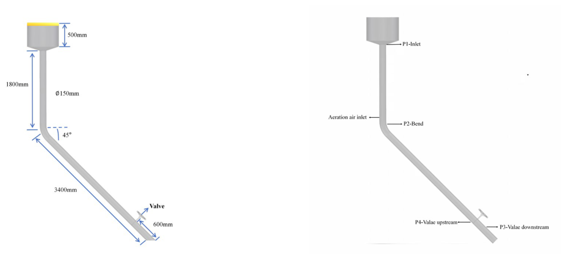
Figure 2.
Computational mesh of the gas–solid flow domain.
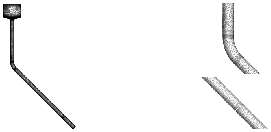
Figure 3.
Experimental regenerated-catalyst standpipe and measurement system.
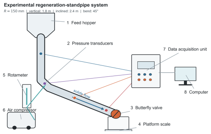
Figure 4.
Experimental–numerical pressure validation: (a) absolute mean gauge pressures, with experimental error bars denoting temporal standard deviations; (b) min–max-normalized pressure response; and (c) 1:1 comparison of the normalized values. Matched condition labels in (a,b) give experimental aeration rate (L h−1) / numerical superficial aeration velocity (m s−1).
Figure 4.
Experimental–numerical pressure validation: (a) absolute mean gauge pressures, with experimental error bars denoting temporal standard deviations; (b) min–max-normalized pressure response; and (c) 1:1 comparison of the normalized values. Matched condition labels in (a,b) give experimental aeration rate (L h−1) / numerical superficial aeration velocity (m s−1).
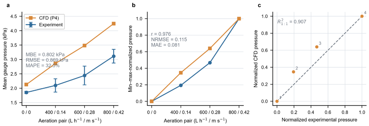
Figure 5.
First six mode shapes of the regenerated-catalyst standpipe.
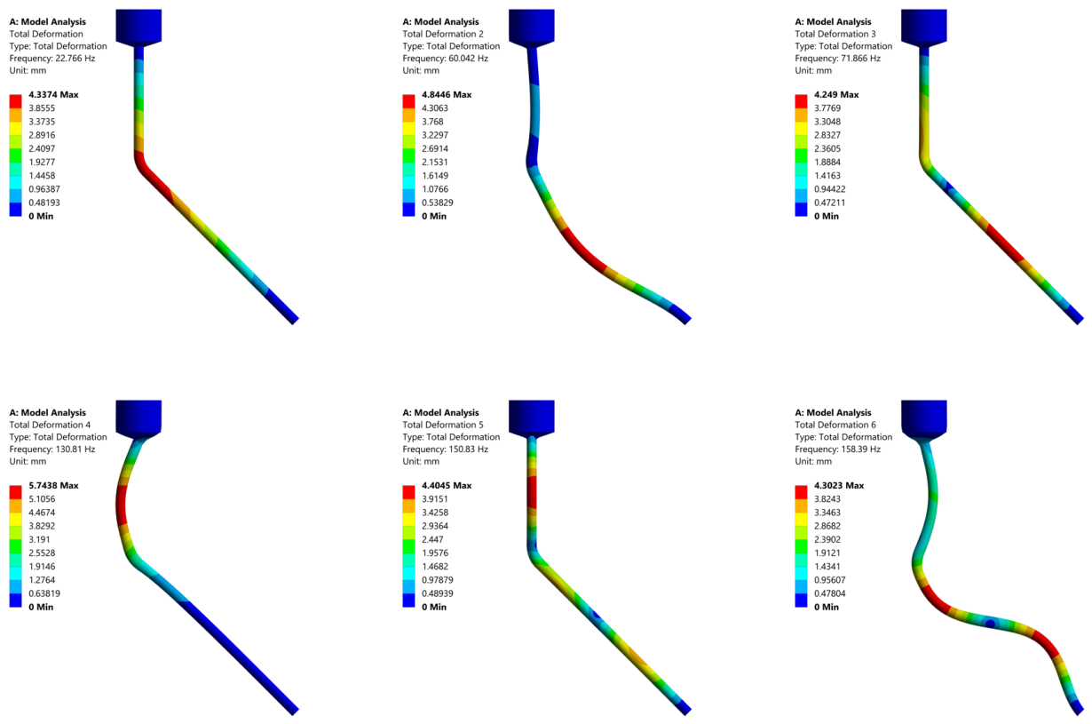
Figure 6.
Effects of pipe diameter and material properties on the first six natural frequencies of the regenerated-catalyst standpipe.
Figure 6.
Effects of pipe diameter and material properties on the first six natural frequencies of the regenerated-catalyst standpipe.
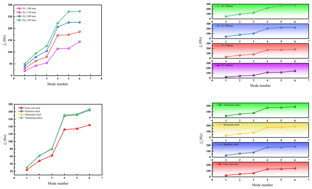
Figure 7.
Random-vibration and harmonic-response results of the regenerated-catalyst standpipe: (a) 3σ equivalent stress under Z-direction excitation; (b) equivalent stress at 180 Hz; (c) total deformation at 180 Hz; and (d) stress and strain amplitudes as functions of excitation frequency.
Figure 7.
Random-vibration and harmonic-response results of the regenerated-catalyst standpipe: (a) 3σ equivalent stress under Z-direction excitation; (b) equivalent stress at 180 Hz; (c) total deformation at 180 Hz; and (d) stress and strain amplitudes as functions of excitation frequency.
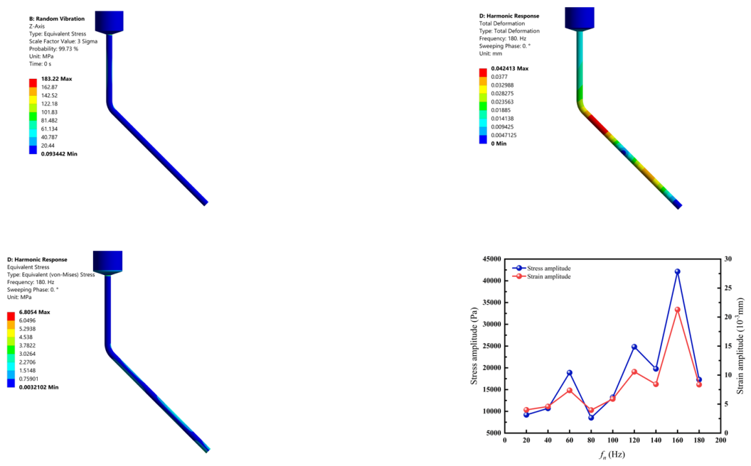
Figure 8.
Time-averaged gauge-pressure distributions for the 16 operating conditions at a butterfly-valve opening of 30%. Rows correspond to Gs = 5, 10, 15, and 20 kg s−1, and columns correspond to ua = 0, 0.14, 0.28, and 0.42 m s−1. A common color scale is used.
Figure 8.
Time-averaged gauge-pressure distributions for the 16 operating conditions at a butterfly-valve opening of 30%. Rows correspond to Gs = 5, 10, 15, and 20 kg s−1, and columns correspond to ua = 0, 0.14, 0.28, and 0.42 m s−1. A common color scale is used.
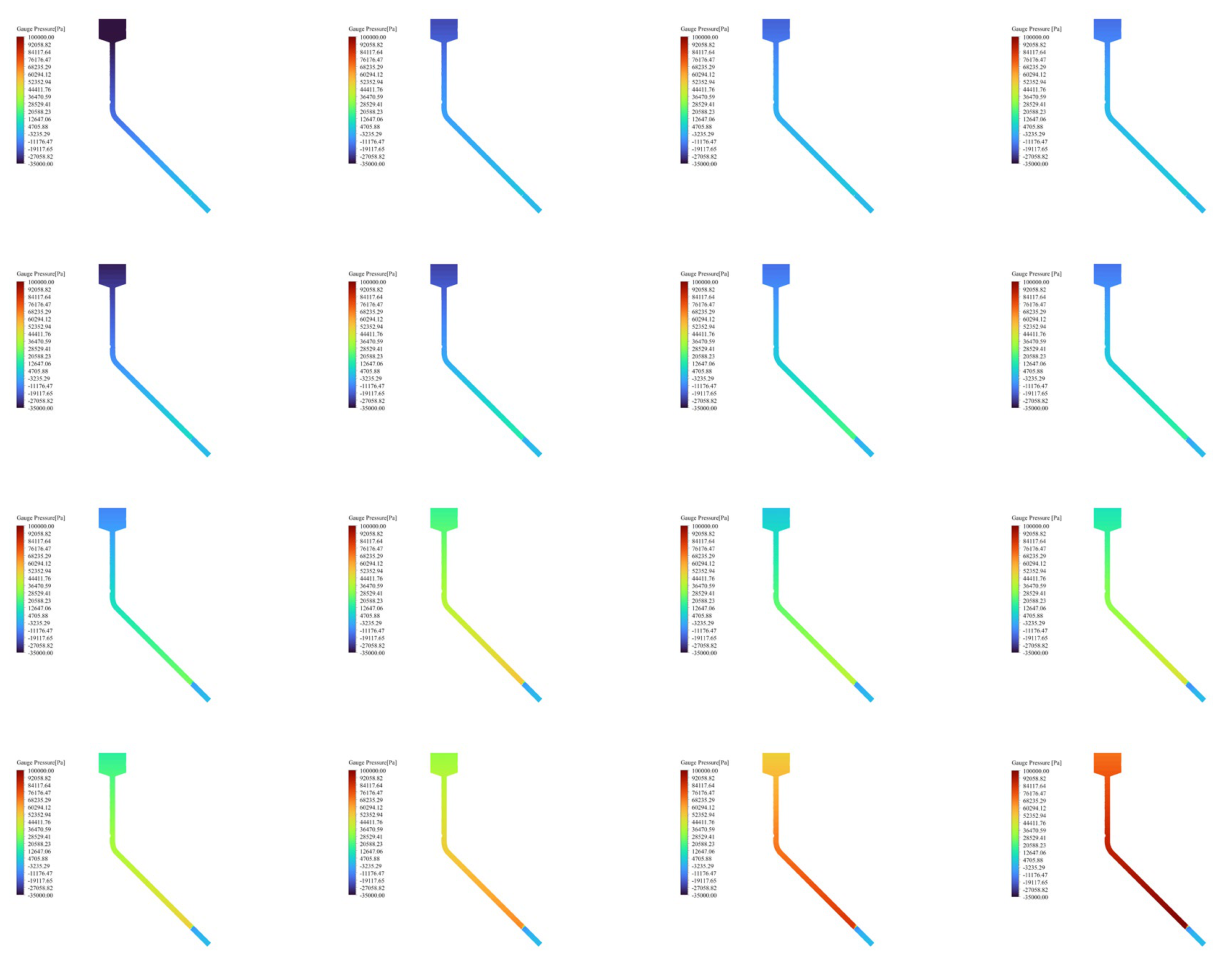
Figure 9.
Solids volume-fraction distributions for the 16 operating conditions. Rows correspond to Gs = 5, 10, 15, and 20 kg s−1, and columns correspond to ua = 0, 0.14, 0.28, and 0.42 m s−1.
Figure 9.
Solids volume-fraction distributions for the 16 operating conditions. Rows correspond to Gs = 5, 10, 15, and 20 kg s−1, and columns correspond to ua = 0, 0.14, 0.28, and 0.42 m s−1.
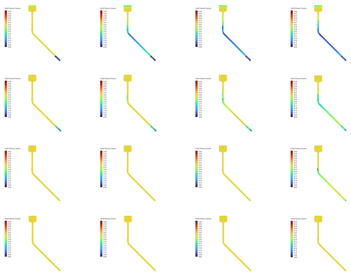
Figure 10.
Gas volume-fraction distributions for the 16 operating conditions. Rows correspond to Gs = 5, 10, 15, and 20 kg s−1, and columns correspond to ua = 0, 0.14, 0.28, and 0.42 m s−1.
Figure 10.
Gas volume-fraction distributions for the 16 operating conditions. Rows correspond to Gs = 5, 10, 15, and 20 kg s−1, and columns correspond to ua = 0, 0.14, 0.28, and 0.42 m s−1.
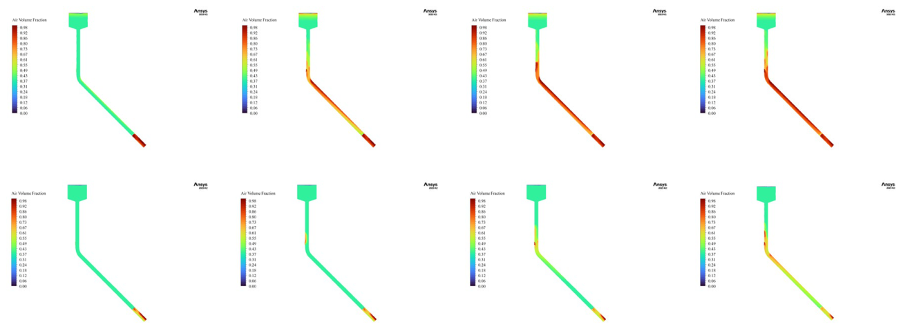
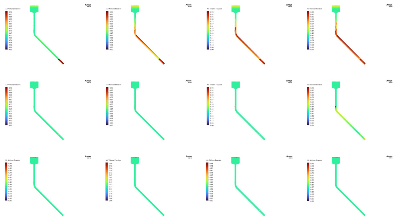
Figure 11.
Gauge-pressure histories at P1–P4 for the 16 operating conditions. Rows correspond to Gs = 5, 10, 15, and 20 kg s−1, and columns correspond to ua = 0, 0.14, 0.28, and 0.42 m s−1. The shaded band denotes the 45–50 s numerical re-equilibration interval excluded from quasi-steady statistics.
Figure 11.
Gauge-pressure histories at P1–P4 for the 16 operating conditions. Rows correspond to Gs = 5, 10, 15, and 20 kg s−1, and columns correspond to ua = 0, 0.14, 0.28, and 0.42 m s−1. The shaded band denotes the 45–50 s numerical re-equilibration interval excluded from quasi-steady statistics.
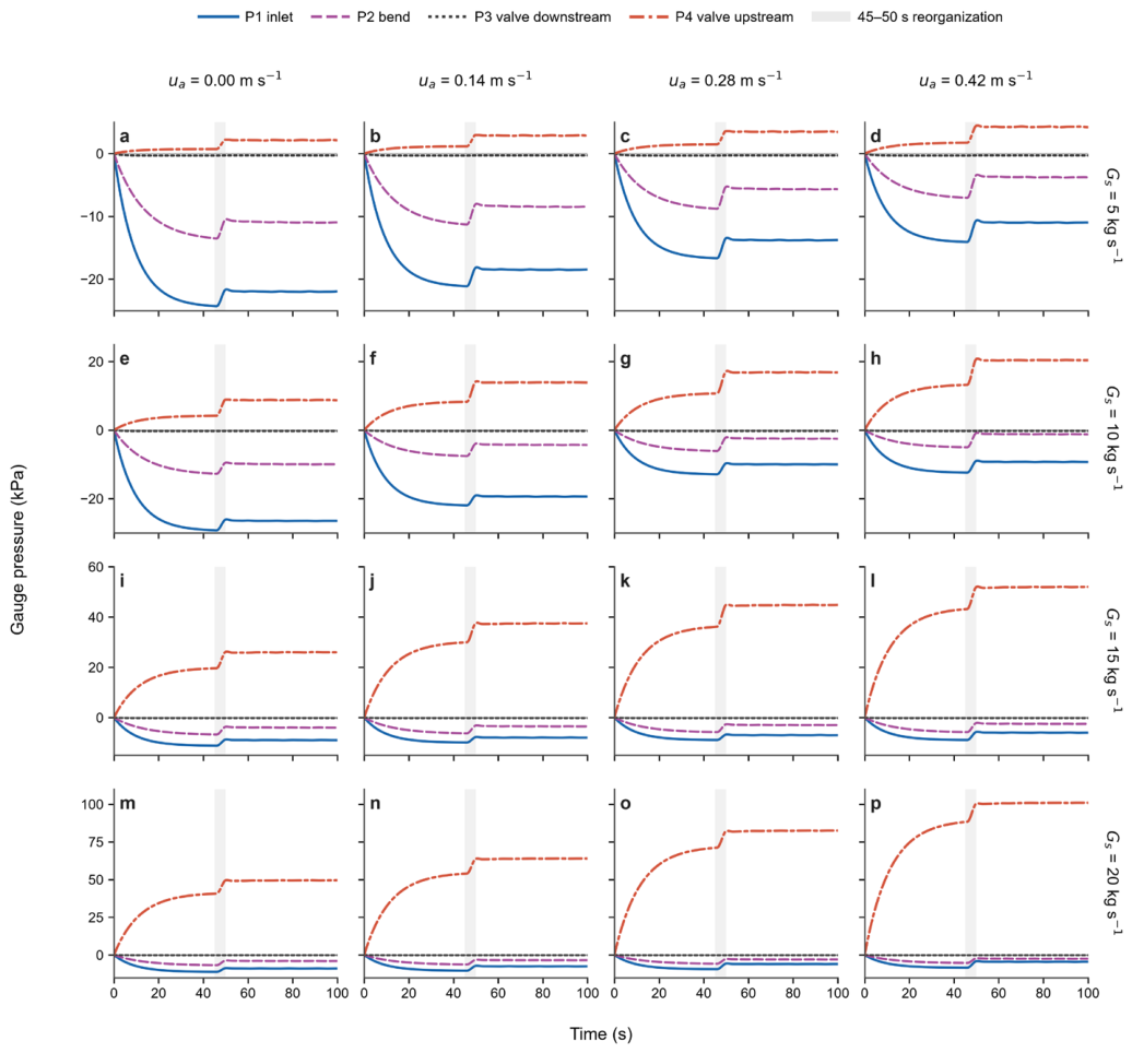
Figure 12.
Structural response of the regenerated-catalyst standpipe under mapped fluid pressure: (a) equivalent stress and (b) total deformation.
Figure 12.
Structural response of the regenerated-catalyst standpipe under mapped fluid pressure: (a) equivalent stress and (b) total deformation.
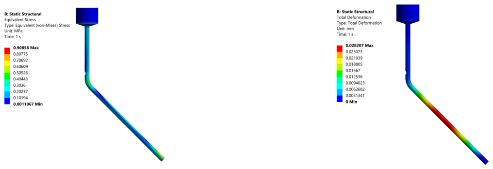

Table 1.
Main geometric parameters of the regenerated-catalyst standpipe.
| Parameter | Value |
|---|---|
| Pipe inner diameter / wall thickness | 150 mm / 5 mm |
| Vertical-section length | 1800 mm |
| Inclined-section length / inclination | 3400 mm / 45° |
| Hopper diameter / height | 700 mm / 500 mm |
| Valve-downstream section length / valve opening | 600 mm / 30% |
Table 2.
Structural mesh-convergence results.
| Mesh | Nodes | Elements | f1 (Hz) | f2 (Hz) | f3 (Hz) | Maximum relative change (%) |
|---|---|---|---|---|---|---|
| Coarse | 512,438 | 125,890 | 23.214 | 61.436 | 73.221 | – |
| Medium | 1,029,489 | 251,646 | 22.766 | 60.042 | 71.866 | 2.32 |
| Fine | 1,452,386 | 361,104 | 22.714 | 59.918 | 71.742 | 0.23 |
Table 3.
Matrix of transient gas–solid operating conditions.
| Gs (kg s−1) | ua = 0 | ua = 0.14 | ua = 0.28 | ua = 0.42 |
|---|---|---|---|---|
| 5 | C01 | C02 | C03 | C04 |
| 10 | C05 | C06 | C07 | C08 |
| 15 | C09 | C10 | C11 | C12 |
| 20 | C13 | C14 | C15 | C16 |
Table 4.
First six natural frequencies and principal mode shapes.
| Mode | Frequency (Hz) | Principal mode shape | Main response region |
|---|---|---|---|
| 1 | 22.766 | First global bending | Vicinity of the bend |
| 2 | 60.042 | First bending of the inclined pipe | Midspan of the inclined pipe |
| 3 | 71.866 | Second bending with an additional node | Bend-inclined-pipe transition |
| 4 | 130.810 | Higher-order local bending | Connection transition |
| 5 | 150.830 | Torsion-dominated mode | Valve connection and vertical section |
| 6 | 158.390 | Coupled bending and torsion | Bend, inclined pipe, and support vicinity |
Table 5.
Maximum 3σ equivalent stress under excitation in different directions.
| Excitation direction | Maximum 3σ equivalent stress (MPa) | Response rank |
|---|---|---|
| X | 46.581 | 3 |
| Y | 140.290 | 2 |
| Z | 183.220 | 1 |
Table 6.
Mean gauge pressures and characteristic pressure differences during the quasi-steady interval of 60–100 s. Means and sample standard deviations were calculated from 81 values per signal at 0.5 s intervals.
Table 6.
Mean gauge pressures and characteristic pressure differences during the quasi-steady interval of 60–100 s. Means and sample standard deviations were calculated from 81 values per signal at 0.5 s intervals.
| Gs | ua | P1 (kPa) | P2 (kPa) | P3 (kPa) | P4 (kPa) | Δpvi (kPa) | Δpvo (kPa) | σp,P4 (Pa) |
|---|---|---|---|---|---|---|---|---|
| 5 | 0.00 | −21.987 | −10.945 | −0.300 | 2.128 | 24.115 | 2.427 | 28.8 |
| 5 | 0.14 | −18.488 | −8.453 | −0.300 | 2.861 | 21.349 | 3.161 | 28.0 |
| 5 | 0.28 | −13.790 | −5.664 | −0.300 | 3.482 | 17.272 | 3.782 | 27.8 |
| 5 | 0.42 | −10.991 | −3.771 | −0.300 | 4.245 | 15.237 | 4.545 | 31.8 |
| 10 | 0.00 | −26.485 | −9.949 | −0.250 | 8.759 | 35.244 | 9.009 | 36.0 |
| 10 | 0.14 | −19.389 | −4.296 | −0.225 | 13.909 | 33.299 | 14.135 | 38.8 |
| 10 | 0.28 | −9.994 | −2.477 | −0.226 | 16.881 | 26.875 | 17.106 | 39.6 |
| 10 | 0.42 | −9.296 | −1.182 | −0.226 | 20.427 | 29.723 | 20.653 | 40.0 |
| 15 | 0.00 | −8.997 | −3.976 | −0.201 | 25.968 | 34.966 | 26.169 | 45.8 |
| 15 | 0.14 | −7.999 | −3.478 | −0.200 | 37.455 | 45.453 | 37.655 | 52.9 |
| 15 | 0.28 | −6.999 | −2.979 | −0.200 | 44.747 | 51.746 | 44.947 | 57.6 |
| 15 | 0.42 | −5.999 | −2.479 | −0.200 | 51.938 | 57.937 | 52.138 | 64.8 |
| 20 | 0.00 | −8.997 | −3.974 | −0.150 | 49.442 | 58.440 | 49.592 | 64.1 |
| 20 | 0.14 | −7.496 | −3.475 | −0.150 | 63.923 | 71.419 | 64.073 | 80.5 |
| 20 | 0.28 | −5.995 | −2.976 | −0.149 | 82.397 | 88.392 | 82.547 | 103.9 |
| 20 | 0.42 | −4.495 | −2.477 | −0.149 | 100.870 | 105.365 | 101.020 | 128.7 |
Disclaimer/Publisher’s Note: The statements, opinions and data contained in all publications are solely those of the individual author(s) and contributor(s) and not of MDPI and/or the editor(s). MDPI and/or the editor(s) disclaim responsibility for any injury to people or property resulting from any ideas, methods, instructions or products referred to in the content. |
© 2026 by the authors. Licensee MDPI, Basel, Switzerland. This article is an open access article distributed under the terms and conditions of the Creative Commons Attribution (CC BY) license (http://creativecommons.org/licenses/by/4.0/).
Copyright: This open access article is published under a Creative Commons CC BY 4.0 license, which permit the free download, distribution, and reuse, provided that the author and preprint are cited in any reuse.