

Submitted:
02 September 2026
Posted:
04 September 2026
You are already at the latest version
Abstract
Unsteady forced convection is almost always computed by inserting a steady velocity field into a time-dependent energy equation, because exact unsteady solutions of the coupled problem are scarce. We remove the inconsistency by transforming the full Navier–Stokes and energy equations—retaining streamwise diffusion, streamwise conduction and the complete dissipation function—under the diffusion-time-scale variables η = y/δ(x), τ = νt/δ(x)2. The energy equation transforms in closed form with the same stretching operator D = η∂η + 2τ∂τ and the same parameters α, β, γ as the momentum equation; the terms in ηfηθη cancel identically, as they do in the momentum balance, and a wall temperature Tw − T∞ ∝ x2m keeps the Eckert number constant and contributes a single extra term 2Prβfηθ. The coupled system closes in (η, τ) alone if and only if m = −1 when dissipation is retained, and for m = ±1 when it is not: the streamwise strain 4u2x carries a coefficient that no choice of scaling removes. Because D annihilates ζ = η/√τ = y/√νt, temperature fields θ = Θ(ζ) reduce the energy equation exactly to Θ′′ + 1/2Prζ Θ′ + π−1PrEc e−ζ2/2 = 0, whose solution is Θ = erfc(√Pr ζ/2)without dissipation and elementary at Pr = 2. Unlike previous unsteady thermal solutions, which satisfy their boundary conditions only as τ → ∞, this one satisfies them exactly at every finite time. It yields Nux = 0.3989(1 − 12Ec r)√PrRex/τ, a heat transfer coefficient independent of x, a recovery factor r = 2√πPrQ(Pr) equal to unity at Pr = 1, and a thickness ratio δT/δu = Pr−1/2 exact at all Pr, with none of the Pr−1/3 crossover of the steady Pohlhausen layer. The stagnation-point member m = 1 is solved numerically and relaxes onto its steady state within one diffusion time. For the fully closing case m = −1, a diverging wedge, the steady thermal problem is shown to coincide exactly with the vorticity equation at Pr = 1, so that the temperature follows by quadrature, and to be of Helmholtz type in general: it loses uniqueness at a discrete set of critical Prandtl numbers, the first at Prc = 1.82 and almost independent of Reynolds number.
Keywords:
2D laminar flow
; exact solutions
; forced convection
1. Introduction
Laminar forced convection is described, in almost every textbook and every engineering correlation, by the pair consisting of the Blasius momentum solution [2] and the Pohlhausen energy solution [9]. Both are steady. When the thermal problem is genuinely time dependent—a plate switched on, a wall temperature stepped, a start-up transient—the standard procedure retains in the energy equation while inserting the steady velocity field.
That procedure is an approximation, and often a good one: when the thermal layer is much thinner than the momentum layer, as at large Prandtl number, the velocity field evolves slowly on the scale that matters for T and the quasi-steady treatment is entirely adequate for engineering purposes. It is nevertheless not self-consistent—a fluid particle cannot convect a time-dependent temperature along a time-independent trajectory—and its accuracy has never been assessed against an exact coupled solution, because none was available. Our object is to supply one: not to displace the quasi-steady approximation, but to give it a benchmark. Exact solutions of the Navier–Stokes equations are rare [16,17,18], and unsteady two-dimensional ones rarer still; the classical analyses of Stokes [13], Rayleigh [10], Stewartson [12], Hall [5], Dennis [3] and Riley [11] produced asymptotic and numerical results, and the group classification of Ma and Hui [8] enumerated the similarity reductions of the boundary-layer system, but the thermal problem inherited the gap of necessity: an exact unsteady temperature field presupposes an exact unsteady velocity field to convect it.
Two developments make the coupled problem tractable. The first is the diffusion-time-scale transformation of Sun [15], which promotes time itself to a similarity variable by measuring it against the transverse diffusion time identified by Stuart [14]. The second is the observation, developed in a companion analysis, that the same transformation applied to the full equations—with no thin-layer approximation—closes only for particular members of the family, and that the stretching operator it generates annihilates a distinguished variable which reduces the problem to an ordinary differential equation.
The present paper carries that programme through for the temperature field. We work throughout with the complete equations: streamwise diffusion , streamwise conduction and the full dissipation function are all retained, so that every statement is a statement about the Navier–Stokes system rather than about a truncation of it. Section 2 sets out the equations and §3 transforms the energy equation. Section 4 establishes the closure condition for the coupled system, which is narrower than for the momentum equation alone, and identifies dissipation as the obstruction. Section 5 obtains the exact solutions, §6 the heat-transfer characteristics, and §7 solves the stagnation-point member numerically. Section 8 concludes.
2. Formulation
A Newtonian fluid of constant density , kinematic viscosity , thermal diffusivity and Prandtl number occupies a two-dimensional region bounded by a wall. The governing equations, complete, are
The dissipation function is with . In two dimensions, using ,
of which the thin-layer approximation retains only . We keep both terms; the first will turn out to control the closure of the coupled problem.
Continuity is satisfied by , . The wall is impermeable and at rest, and we consider the isothermal and adiabatic conditions
with far from the wall.
3. Transformation of the Energy Equation
3.1. Variables and the Stretching Operator
Following Sun [15] we set
Since and , all streamwise chain rules collapse onto the stretching operator
and for any and any ,
with . The velocity components are
where, as in the momentum problem,
and constancy of these forces the power-law family
Three derived quantities recur below:
being the local Reynolds number, together with , which measures the size of the streamwise-diffusion and streamwise-conduction terms.
3.2. The Wall Temperature Scale
Write
The Eckert number is constant if and only if , that is
This is a genuine extension of the isothermal case: holding fixed forces and restricts the reduction to the flat plate, whereas (15) admits the whole family. For it reduces to a uniform wall temperature.
3.3. The Cancellation
Both contain : the first through , the second through the inside V. Since the two contributions are and cancel identically. This is the same cancellation that makes the momentum equation reduce, and it is the step most easily lost: differentiating f with respect to x through only, and not through , leaves a spurious and destroys every reduction below.
3.4. The Transformed Equation
Multiplying (4) by and collecting gives the exact transformed energy equation
with the transformed dissipation
The first group on the right of (17) is transverse conduction, the second streamwise conduction , the third dissipation. The term is contributed by the varying wall temperature and vanishes for the flat plate. Setting , and retaining only in (18) recovers the thin-layer form of the transformed energy equation.
Two independent checks were made. At , , the streamwise velocity is itself a passive scalar, and setting in (17) returns the momentum equation exactly; with the spurious term retained it does not. Separately, (17) was verified against (4) in physical variables for , using none of the algebra above (Appendix A).
4. Closure of the Coupled System
The parameters are constants by construction. The reduction to two independent variables therefore requires that the remaining coefficients in (17)–(18) be free of x. There are three, and since they are
all proportional to . The first two carry a factor n and therefore vanish identically when , that is ; the third does not.
Theorem 1.
Under the transformation (7) with , the coupled system (1)–(4) reduces to two independent variables if and only if
- 1.
- , when viscous dissipation is retained; or
- 2.
- or , when dissipation is absent .
Proof.
The theorem is sharper than the corresponding statement for the momentum equation alone, which admits both . The obstruction is the term in (5), discarded in every thin-layer treatment: the streamwise strain heats the fluid at a rate that does not scale with the transverse shear, and only a geometry in which is constant—a diverging or converging wedge, —keeps the two in proportion.
The case singled out by the theorem deserves comment, since we do not solve it here. For one has , and constant: the flow occupies a wedge whose walls are surfaces of constant , and the wall temperature varies as . The steady limit is Jeffery–Hamel flow [6,7] with heat transfer, and is an ordinary differential system. The unsteady problem is harder, and in a way that is structural rather than technical: with finite, the streamwise second derivatives make the reduced system elliptic in , with principal symbol where . The similarity time is then not an evolution variable: data must be posed at both ends of the interval, the line is characteristic and admits fewer conditions than an elliptic boundary would, and marching is inconsistent. Whether the temperature field inherits the upstream influence of the velocity field, and how it behaves near the Jeffery–Hamel bifurcation where the steady solution loses uniqueness [1,4], are open questions that we regard as the natural continuation of this work.
Remark 1.
The case , the flat plate, closes only in the thin-layer sense: the streamwise conduction and streamwise strain both survive with coefficients . It is nevertheless the case for which exact solutions are available, because those solutions annihilate the offending groups individually (§5).
5. Exact Solutions
5.1. The Invariant Variable
Because assigns weight 1 to and 2 to , the ratio
independently of and hence of x. Temperature fields of the form are therefore group invariant, and three simplifications follow at once. The Jacobian term combines with into whenever the velocity field satisfies , and then vanishes. The streamwise conduction group reduces to a multiple of ,
which vanishes if or , that is or . And the term carries an explicit unless .
The three conditions are met simultaneously by the branch , , that is the flat plate, on which the companion momentum analysis gives the exact velocity field
the Rayleigh–Stokes layer, which satisfies the no-slip and outer conditions exactly at every finite .
5.2. Reduction of the Energy Equation
Theorem 2.
Proof.
Equation (23) is the unsteady counterpart of the Pohlhausen equation. The correspondence is instructive: in the steady problem the coefficient of is , the Blasius function, known only numerically, whereas here it degenerates to the linear function . That degeneracy is what makes the solutions below elementary while their steady analogues are not.
5.3. Solutions
Equation (23) is linear with integrating factor , so
Imposing , and interchanging the order of integration gives the wall gradient
where ; the scaled form is used because the unscaled kernel overflows for .
For the solution is a complementary error function of the group invariant,
which satisfies and exactly, at every finite τ. This is worth emphasising. Previous unsteady thermal solutions built on the Kummer-function branch of the velocity field satisfy their boundary conditions only as , with a defect of ; here there is no defect, because the underlying velocity field (22) has none.
At the integral in (24) is elementary and the full solution with dissipation closes:
Profiles for general and are shown in Figure 1.
6. Heat Transfer Characteristics
The wall heat flux follows from , using , so that with ,
or equivalently, in purely temporal form,
which is independent of x: a signature of the Rayleigh-type structure of the unsteady layer, and a qualitative departure from the steady law.
For an adiabatic wall, in (24) with gives the recovery factor
being the Eckert number at which (28) vanishes and the heat flux reverses. The identity states that reversal occurs when , as it must. At we find exactly, hence
recovering the classical unit recovery factor. Values are given in Table 1.
6.1. Limits of the Recovery Factor
Both limits of Q are analytic. As the kernel and
so the classical scaling is recovered with prefactor in place of unity. As the kernel behaves as , the integral is cut off at , and the logarithmic divergence of gives
Numerically the fitted slope over is against , and (33) reproduces the computed values to over that range. The logarithmic growth is a genuinely unsteady effect: dissipation is confined to a Stokes sublayer of thickness while the thermal layer shrinks as , so their overlap saturates instead of following the steady law. Both limits are shown in Figure 1(c).
Defining thicknesses through and gives, exactly and at all ,
This is worth contrasting with the steady Prandtl–Blasius layer, in which the corresponding ratio crosses over from at small to at large . No crossover occurs here: both layers are diffusive rather than convective in structure, and the single exponent registers that difference. The exponent itself is not new—the same appears in the thermal analogues of the Rayleigh and Stokes problems [10,13], for the same reason, both layers there being purely diffusive. What is new is that it holds here for a genuinely two-dimensional flow with a nontrivial transverse velocity, where one would expect convection to reinstate the crossover; the reason it does not is that the convective operator is annihilated on -invariant fields, so the temperature never feels the velocity field except through the dissipation term.
7. The Stagnation-Point Member: A Numerical Example
The case is, by the theorem of §4, an exact reduction of the full system whenever dissipation is absent. Here , , , is constant and , the velocity field is , with identically, and the wall temperature varies as . Equation (17) collapses to
coupled to the momentum equation . Both are parabolic in , because removes the elliptic contribution, so the pair may be marched.
We integrate from an impulsive start, and for at , with . Physically this is the stagnation-point analogue of the impulsively started plate [5,12]: at the fluid is in the inviscid straining motion , everywhere and at the ambient temperature, and at the wall is brought to rest and to simultaneously. Both fields therefore begin with a discontinuity at the wall, and both initially diffuse one-dimensionally, which is the origin of the short-time laws below. It differs from the classical problem in that the outer flow here strains as well as convects, so the layer reaches a steady thickness instead of growing indefinitely. The integration uses second-order central differences in and implicit stepping in , with Newton iteration for the momentum equation and a direct tridiagonal solve for (35). Results for air are shown in Figure 2.
Two limits are recovered. As ,
the one-dimensional conduction law, the computed value at being against ; the convective and wall-temperature terms in (35) have not yet acted. As the solution relaxes onto its steady state, with
the latter reproducing the Hiemenz value to six figures and providing an independent check on the coupled solver. The relaxation is complete to three figures by , that is after one diffusion time ; the thermal field lags the velocity field slightly, the ratio in Figure 2(b) settling later than either quantity separately.
8. The Fully Closing Case
Theorem 1 singles out as the only member for which the coupled system closes with dissipation retained, and it would be unsatisfactory to leave that case untouched. Here , , , , and is a genuine constant; the walls are surfaces of constant , so the flow occupies a wedge of half-angle , and (15) requires a wall temperature . We take the steady problem, which is an ordinary differential system, and record what it implies for the unsteady one.
8.1. The Steady Thermal Problem
With the operator becomes , and (17) reduces to
with
the second group being the streamwise-strain contribution that Theorem 1 identifies as the obstruction at . The velocity field is the Jeffery–Hamel solution [6,7], obtained from together with . Equation (38) is linear in , so it may be solved directly once f is known.
8.2. An Exact Correspondence at
Comparison of (38) at , with the vorticity equation above shows that the two are identical. The temperature and the vorticity therefore satisfy the same second-order operator, and is a known solution of the homogeneous thermal problem. Reduction of order then supplies the general solution by quadrature,
the weight following from with . Numerically, imposing ’s own boundary values reproduces to , which is a stringent check on both solvers. Equation (40) is the analogue of the unsteady Reynolds analogy: at unit Prandtl number the thermal field is slaved to the vorticity field, not to the velocity field, because the wall temperature and the vorticity decay downstream at the same rate. The quadrature is singular where vanishes, which for a diverging wedge occurs once inside the channel; the combination remains regular there, but the two branches must be matched across the zero.
8.3. Loss of Uniqueness at Critical Prandtl Numbers
The zeroth-order coefficient in (38) is , which is positive whenever the flow is unseparated. Equation (38) is therefore of Helmholtz type rather than of maximum-principle type, and the homogeneous problem possesses nontrivial solutions at a discrete set of Prandtl numbers. Solving the generalised eigenvalue problem
at , gives, grid-converged on 400, 800 and 1600 intervals,
Below the first of these the boundary-value problem is uniquely solvable; at it is solvable only if the dissipation term satisfies a compatibility condition, and the wall gradient diverges as approaches from below, taking the values , , and at , , 1 and .
The first critical value is strikingly insensitive to the Reynolds number, moving only from to as varies from to 40 (Figure 3c); the higher modes fall slowly with . This mirrors, in the thermal problem, the non-uniqueness that Jeffery–Hamel flow itself exhibits above a critical Reynolds number [1,4], and it arises from the same feature of the geometry: the streamwise decay required by (15) acts as a distributed source in the frame of the moving fluid, and at discrete that source resonates with the diffusive operator. Profiles below the first critical value, with and without dissipation, are shown in Figure 3(a,b).
8.4. The Unsteady Problem
For the unsteady problem at the coefficient is finite, so the streamwise second derivatives survive and the reduced system is elliptic in , with principal symbol , , degenerating only on . The similarity time is then not an evolution variable: data must be posed at both ends of the interval, the line is characteristic and admits fewer conditions than an elliptic boundary, and marching in is inconsistent. The temperature field inherits this structure through the same groups. Whether the critical Prandtl numbers (42) survive as genuine bifurcations of the unsteady problem, or are smoothed by the ellipticity, is the natural next question; we have not attempted it here.
9. Discussion and Conclusions
Applying the diffusion-time-scale transformation to the complete Navier–Stokes and energy equations gives (17), in which the energy equation carries the same operator and the same parameters as the momentum equation, the terms in cancelling identically. A wall temperature keeps the Eckert number constant and contributes one further term .
The principal structural result is the closure theorem of §4. With dissipation retained the coupled system reduces to two variables only for ; the obstruction is the streamwise strain , discarded in every thin-layer treatment, whose coefficient carries no factor of n and therefore survives at . Dropping dissipation restores the second case. This is narrower than the closure condition for the momentum equation alone, and it identifies precisely which neglected term is responsible.
The principal explicit result is the exact solution (26)–(27). Because annihilates , invariant temperature fields reduce the energy equation to the elementary linear equation (23), whose solution is a complementary error function without dissipation and closes in elementary functions at . Unlike previous unsteady thermal solutions, it satisfies its boundary conditions exactly at every finite time rather than asymptotically, because the velocity field on which it is built does so. It yields a heat transfer coefficient independent of x, a recovery factor equal to unity at , and a thickness ratio exact at all Prandtl numbers, with none of the crossover of the steady layer.
We would not present these results as a reason to abandon the quasi-steady treatment, which remains accurate wherever the velocity field evolves slowly on the thermal time scale, and which is far simpler to apply. Their value is as a benchmark: an exact, fully coupled solution of the unsteady problem against which the quasi-steady approximation, and unsteady numerical schemes, can be calibrated. Equation (28) in particular provides a closed-form target with no adjustable constants.
Three limitations should be stated. The solution (26) describes a layer that grows as and does not saturate at the Blasius thickness: it is an exact member of a class of unsteady layers, not a description of the complete Rayleigh-to-Blasius transition. The unsteady form of the case is an elliptic boundary-value problem in rather than an evolution problem, and only its steady limit is solved here. And the results of §6 assume constant properties throughout.
The mechanism identified in §5 is not special to this flow. Whenever a solution is invariant under a one-parameter group, the convective operator restricted to invariant scalars loses its dependence on the velocity field, and any passive scalar reduces to an ordinary differential equation with the flow entering only through the source term. That observation should apply equally to species transport, to the three-dimensional problem, and to any other reduction in which a distinguished invariant of the stretching operator can be identified.
Author Contributions
Bo Hua Sun: Conceptualization, Methodology, Formulations, Formal analysis, Funding acquisition, Investigation, Writing- Original draft preparation, Writing- Reviewing and Editing and all relevant works.
Data Availability Statement
The data supporting the findings of this study are available from the corresponding author upon reasonable request.
Acknowledgments
My investigations into the boundary layers started from my tenure as a professor at the Cape Peninsula University of Technology (CPUT), South Africa. I am profoundly grateful to CPUT for granting me complete academic autonomy to advance this research agenda. This vital institutional support laid the foundation for the principal conclusions presented in this manuscript. I also extend my deepest gratitude to former Vice-Chancellor (now Chancellor) Prof. Brian Figaji, and former Deputy Vice-Chancellors Prof. J. A. Tromp and Prof. Anthony Staak, for their generous support and endorsement. Further academic support was provided by Xi’an University of Architecture and Technology (XAUAT) and the Beijing Institute of Nanoenergy and Nanosystems (BINN), Chinese Academy of Sciences. I sincerely thank former XAUAT President Prof. Xiao-Jun Liu and current President Prof. Xiang-Mo Zhao, along with BINN Founding Director Prof. Zhong Lin Wang, for their unwavering encouragement and invaluable resource support throughout this study.
Conflicts of Interest
The authors declare that there are no competing financial interests.
Appendix A. Verification
Every relation quoted above was checked by two independent routes.
Symbolic. The convective operator of (17) was formed from with and shown to equal identically. The identity on the branch (22) was verified, and substituting into (17) was shown to reproduce (23) with zero residual. The closed form (27) annihilates (23) identically and meets both boundary conditions.
Physical variables. For the fields u, v and were assembled in coordinates from an arbitrary analytic f and , and the original energy equation (4) evaluated directly; it agrees with (35) scaled by to machine precision, using none of the transformation algebra.
Quadratures. The kernel of (25) overflows for in its unscaled form and is evaluated as , which is bounded on . The value , giving exactly, provides a check on the quadrature.
Numerics. The coupled solver of §7 reproduces the Hiemenz value to six figures in the steady limit, and the short-time behaviour of both fields follows the one-dimensional laws and to within at .
References
- Banks, W. H. H.; Drazin, P. G.; Zaturska, M. B. On perturbations of Jeffery–Hamel flow. J. Fluid Mech. 1988, 186, 559–581. [Google Scholar] [CrossRef]
- Blasius, H. Grenzschichten in Flüssigkeiten mit kleiner Reibung. Z. Für Math. Und Phys. 1908, 56, 1–37. [Google Scholar]
- Dennis, S. C. R. The motion of a viscous fluid past an impulsively started semi-infinite flat plate. J. Inst. Math. Its Appl. 1972, 10, 105–117. [Google Scholar] [CrossRef]
- Fraenkel, L. E. Laminar flow in symmetrical channels with slightly curved walls. I. On the Jeffery–Hamel solutions for flow between plane walls. Proc. R. Soc. Lond. A 1962, 267, 119–138. [Google Scholar] [CrossRef]
- Hall, M. G. The boundary layer over an impulsively started flat plate. Proc. R. Soc. Lond. A 1969, 310, 401–414. [Google Scholar] [CrossRef]
- Hamel, G. Spiralförmige Bewegungen zäher Flüssigkeiten. Jahresber. Der Dtsch. Math.-Ver. 1917, 25, 34–60. [Google Scholar]
- Jeffery, G. B. The two-dimensional steady motion of a viscous fluid. Philos. Mag. 1915, 29, 455–465. [Google Scholar] [CrossRef]
- Ma, P. K. H.; Hui, W. H. Similarity solutions of the two-dimensional unsteady boundary-layer equations. J. Fluid Mech. 1990, 216, 537–559. [Google Scholar] [CrossRef]
- Pohlhausen, K. Zur näherungsweisen Integration der Differentialgleichung der laminaren Grenzschicht. Z. Für Angew. Math. Und Mech. 1921, 1, 252–268. [Google Scholar] [CrossRef]
- Rayleigh, Lord. On the motion of solid bodies through viscous liquid. Philos. Mag. 1911, 21, 697–711. [Google Scholar] [CrossRef]
- Riley, N. Unsteady laminar boundary layers. SIAM Rev. 1975, 17, 274–297. [Google Scholar] [CrossRef]
- Stewartson, K. On the impulsive motion of a flat plate in a viscous fluid. Q. J. Mech. Appl. Math. 1951, 4, 182–198. [Google Scholar] [CrossRef]
- Stokes, G. G. On the effect of the internal friction of fluids on the motion of pendulums. Trans. Camb. Philos. Soc. 1851, 9, 8–106. [Google Scholar]
- Stuart, J. T. Unsteady boundary layers. In Laminar Boundary Layers; Rosenhead, L., Ed.; Clarendon Press: Oxford, 1963; pp. 349–408. [Google Scholar]
- Sun, Bo Hua. Similarity solutions of a class of unsteady laminar boundary layer. Phys. Fluids 2024, 36, 083616. [Google Scholar] [CrossRef]
- Wang, C. Y. Exact solutions of the unsteady Navier–Stokes equations. Appl. Mech. Rev. 1989, 42, S269–S282. [Google Scholar] [CrossRef]
- Wang, C. Y. Exact solutions of the steady-state Navier–Stokes equations. Annu. Rev. Fluid Mech. 1991, 23, 159–177. [Google Scholar] [CrossRef]
- Wang, C. Y. Essential Analytic Laminar Flow; Springer Nature: Cham, 2024. [Google Scholar]
Figure 1.
(a) Temperature profiles (26) at ; the dotted curve is the velocity profile . (b) Effect of dissipation at ; at the wall gradient vanishes and beyond it the wall is heated by the fluid. (c) Recovery factor from (30) and reversal threshold from (28), with the small- and large- limits (32) and (33). The curve marked is the recovery factor of the steady Prandtl–Blasius layer [9], shown for comparison.
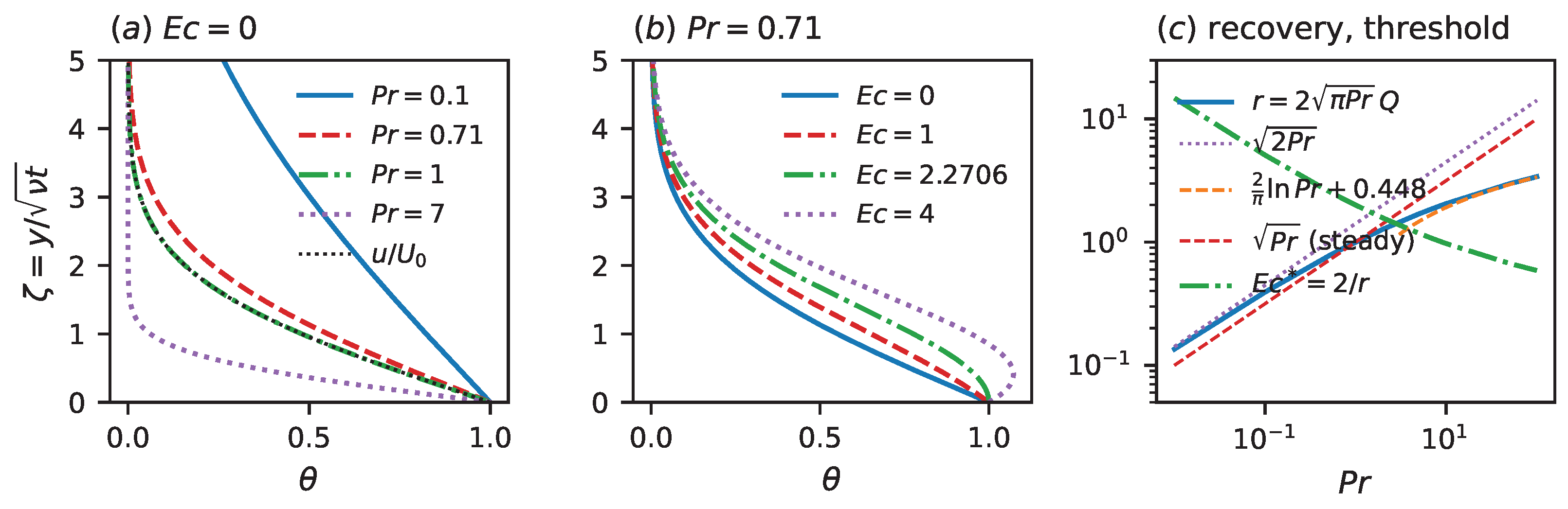
Figure 2.
Unsteady stagnation-point thermal layer, , , . (a) Wall temperature gradient and wall shear against , with the short-time law and the steady limit (dotted). (b) Their ratio, an unsteady Reynolds analogy factor, approaching .
Figure 2.
Unsteady stagnation-point thermal layer, , , . (a) Wall temperature gradient and wall shear against , with the short-time law and the steady limit (dotted). (b) Their ratio, an unsteady Reynolds analogy factor, approaching .
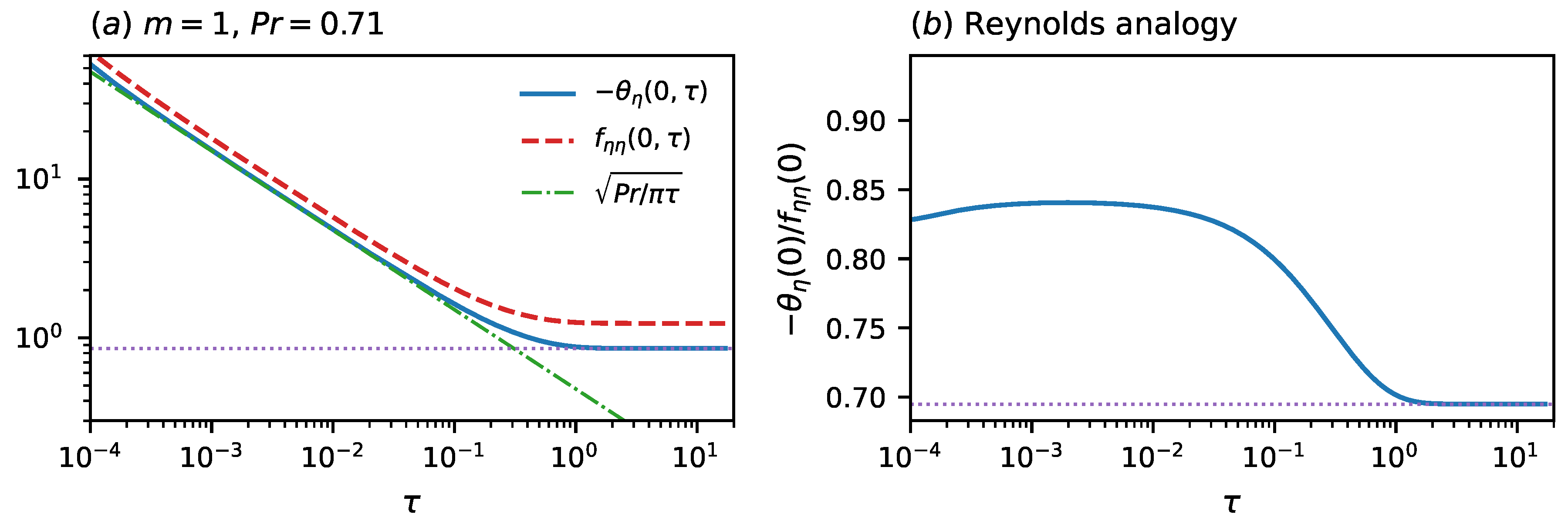
Figure 3.
The fully closing case , a diverging wedge at , , . (a) Temperature profiles (38) at for Prandtl numbers below the first critical value ; the dotted curve is the normalised velocity profile. (b) Effect of viscous dissipation at , with the streamwise-strain contribution of (39) retained. (c) The first three critical Prandtl numbers (42) against Reynolds number; the lowest is nearly independent of .
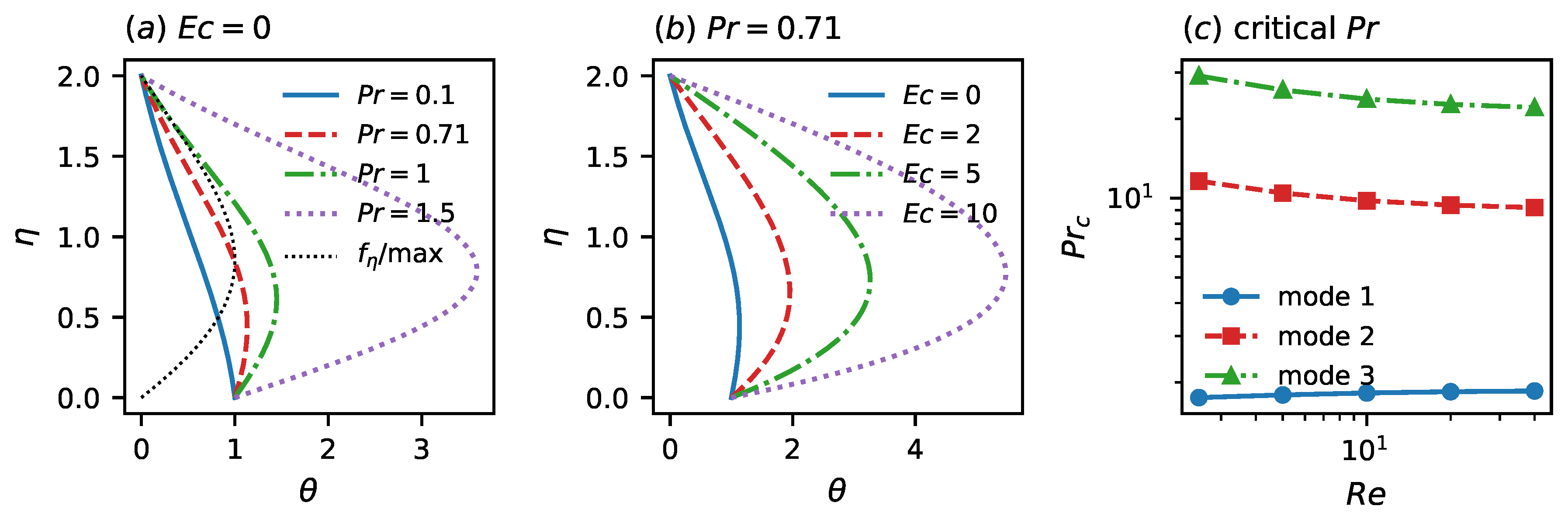

Table 1.
Heat-transfer quantities as functions of the Prandtl number. is the wall temperature gradient at ; Q, defined by the quadrature (25), is the quantity through which dissipation enters, and determines both the recovery factor of (30) and the reversal threshold . The thickness ratio is (34). At , exactly and .
| Q | r | ||||
|---|---|---|---|---|---|
| 1 | |||||
| 2 | |||||
| 5 | |||||
| 7 | |||||
| 10 | |||||
| 50 | |||||
| 100 |
Disclaimer/Publisher’s Note: The statements, opinions and data contained in all publications are solely those of the individual author(s) and contributor(s) and not of MDPI and/or the editor(s). MDPI and/or the editor(s) disclaim responsibility for any injury to people or property resulting from any ideas, methods, instructions or products referred to in the content. |
© 2026 by the author. Licensee MDPI, Basel, Switzerland. This article is an open access article distributed under the terms and conditions of the Creative Commons Attribution (CC BY) license.
Copyright: This open access article is published under a Creative Commons CC BY 4.0 license, which permit the free download, distribution, and reuse, provided that the author and preprint are cited in any reuse.