

Submitted:
02 September 2026
Posted:
03 September 2026
You are already at the latest version
Abstract
Multi-objective rule-curve optimization with metaheuristic algorithms is widely used to improve reservoir release decisions under fluctuating water management conditions. The practical value of the results depends primarily on the correctness of the problem formulation, while the reported results are rarely verified retrospectively for whether they can be translated into actual operation. This study selected the Nam Mang 3 hydropower system in Lao PDR, which pairs a main reservoir for energy production with a regulating pond that controls releases to the downstream river. The operation model was reconstructed and verified from the recorded results, and the problem formulation was diagnosed with a six-tool protocol, applied to the Pareto and representative solutions of seven metaheuristic algorithms (NSGA-II, ALO, CS, GOA, GWO, MVO, and SSA) and cross-checked against the design plan table and actual production records. The diagnostic protocol successfully identifies the structural conditions that must be improved before the newly developed reservoir rule curves are adopted as actual operating rules. The two tiers of the system exhibit symmetrically opposite characteristics: the main tier is over-determined (energy spans only 0.165 percent, and the existing policy lies outside the search bounds at 20 of 24 positions), while the pond tier is under-determined (without constraints or a mass balance, and with energy 1.78 times the mean observed production). Both findings point directly to the required improvements. The study therefore proposes a complete two-tier formulation that restores the pond mass balance, release coupling, and constraints, together with six improvement criteria with verifiable numerical targets, as the basis for the subsequent optimization of regulating pond operation.
Keywords:
problem formulation
; water–energy nexus
; Nam Mang 3
; regulating pond
; excess release
; metaheuristic algorithms
; hypervolume
1. Introduction
Hydropower generation is a key component of the energy systems of the Greater Mekong Subregion and plays an increasing role in the regional transition toward a low-carbon energy system [1,2]. The Lao People’s Democratic Republic (Lao PDR) holds a prominent position in this context, as its topography and runoff regime favor hydropower development for both domestic energy security and electricity export [3,4]. However, how much of the installed potential is converted into actual energy depends primarily on the reservoir operating policy, not on the size of the structure alone. Operating rule curves, which specify the target storage volume for each period of the year, are therefore the principal tool that operators use to make release decisions under runoff uncertainty [5,6,7]. In practice, most rule curves are derived from preliminary design studies combined with operational experience, and they are often applied for long periods without a systematic review of whether they still exploit the full potential of the system [8]. Over the past two decades, the use of simulation and optimization frameworks to revisit existing rule curves has therefore attracted growing attention [9,10,11,12], and this trend raises a methodological question that increasingly requires a clear answer: how should the reliability of the results reported by such studies be verified?
The literature in this field follows a fairly uniform pattern. Several metaheuristic algorithms are applied to the same problem under an identical simulation model, the same decision variables, and the same stopping criterion, and their performance is then ranked with indicators such as the hypervolume (HV) or convergence behavior [13,14]. This pattern yields valuable information on computational performance, yet it gives more weight to the quality of the algorithms than to the structure of the problem being solved, and most studies still lack four checks that should be performed systematically [15,16]. The first is verifying that the reported solutions actually satisfy the constraints declared by the study itself [17]. This check is particularly important because the exterior penalty function method is the most widely used constraint-handling mechanism, and the magnitude of the penalty term and the residual constraint violation in the final solutions are often left unreported [18]. The second is placing the existing operating policy in the same objective space as the optimized solutions, which is necessary for judging whether the claimed improvement actually occurs [16,19]. The third is confirming that every component of the model can express its behavior at the time step that the model adopts [20]. The fourth is examining whether the stated objectives truly conflict to a degree that makes the multi-objective formulation meaningful, or whether they are merely functions of the same variable set responding in the same direction [21]. As a consequence, a typical reader cannot judge from the reported content whether the presented solutions are feasible, even though feasibility is the most fundamental condition for the validity of the results [22,23,24].
The Nam Mang 3 (NM3) reservoir system in Lao PDR is particularly well suited to examining the issues raised above, because it has two structural properties that make the choice of problem formulation strongly influence the results. First, the system is a diversion-type hydropower project with an effective head of approximately 544 m, whereas its operating range spans only 9 m. The head variation is therefore very small relative to the total head, and the energy produced is almost directly proportional to the volume of water passing through the turbines. The nonlinearity between storage and energy, which motivates a large body of work in the literature, thus plays only a minor role in this type of system [20,25]. Second, the system consists of two storage tiers: a main reservoir that provides seasonal storage, and a regulating pond (re-regulation pond) with a small capacity that smooths the supply of water to the turbines over short periods. The two components therefore have distinct characteristic time scales, and the time step chosen for the model inevitably determines which component can express its behavior [26]. Together, these two properties define the mathematical character of the problem before any algorithm is selected: the two-tier structure relates directly to the identifiability of the decision variables, while the nearly constant head relates directly to the degree of conflict between the objectives. The system therefore provides a stringent test case for showing that problem formulation matters no less than the choice of search method [27].
The four neglected checks are not isolated shortcomings. They correspond to four technical mechanisms, each of which can, on its own, make the reported trade-off surface incorrect [15,16]. The first mechanism is the mis-specification of the feasible set. The shape constraints force each rule curve to decrease monotonically to a minimum at a fixed month and then to increase until the end of the year, which embeds the prior assumption that the system performs exactly one drawdown and one refill per year with no drawdown after the wet season. This assumption contradicts reservoir operation in monsoon basins, where storage must be drawn down after the wet-season peak to prepare empty volume for the following year [28,29]. Physically feasible policies, including the existing one, therefore fall outside the self-defined feasible set. The second mechanism arises from a property of the exterior penalty function method, which merges true performance and residual constraint violation into a single value that cannot be separated afterward. The limiting case that deserves attention occurs when the penalty term does not respond to the decision variables: the search then proceeds as if it were unconstrained, while the reported values still appear in penalized form [18]. The third and fourth mechanisms share a common root in the relationship between system structure and problem formulation. When the active capacity of a storage component is substantially smaller than the volume that passes through it within one time step, the component fills and empties completely within a single step, and the decision variables of that tier become structurally unidentifiable, in a manner comparable to insensitive parameters in hydrological model calibration [30]. Likewise, when the head is nearly constant, energy and excess release are both functions of the same release sequence, so the trade-off surface collapses toward a single value in one objective dimension and reflects stochastic variation rather than a genuine trade-off [16]. The common property of the four mechanisms is that their outcome is indistinguishable from a correct result when judged from what an article reports under current practice.
Given these mechanisms, the research problem of this study is to verify the validity of previously reported rule-curve optimization results using only the information contained in the report itself [8]. This problem points to a gap with two layers: a methodological gap, in that no systematic protocol yet exists for the retrospective verification of reported results, even though the necessary information (the objective values in both penalized and unpenalized form, the decision-variable values, and the time series of storage and release) usually appears in the previous research [11,13,19]; and a formulation gap, in that no condition yet links the capacity of each storage tier to the time step of the model [31]. To close both gaps, this study assembles a set of arithmetic tools into a single protocol, grouped by the mechanism that each tool is designed to detect: a mass-balance closure test as the shared foundation for inferring the equations that the model actually uses; the re-evaluation of constraints from the reported variables together with a dominance check that includes the existing policy, for the first mechanism; the recovery of a cross-checkable penalty term from both objectives together with an identity test of the quantities in the result tables, for the second; the time-scale admissibility condition together with a bound-pinning check, for the third; and a geometric analysis of the trade-off surface, for the fourth. In parallel, the study proposes mass-balance equations for the regulating pond that are consistent with the time-scale condition, as the correct form of problem formulation for multi-tier storage systems [31].
This study therefore develops this retrospective diagnostic protocol and applies it to the recorded results of a multi-objective rule-curve optimization of the NM3 reservoir system, which employed seven metaheuristic algorithms: the Non-dominated Sorting Genetic Algorithm II (NSGA-II), the Ant Lion Optimizer (ALO), Cuckoo Search (CS), the Grasshopper Optimization Algorithm (GOA), the Grey Wolf Optimizer (GWO), the Multi-Verse Optimizer (MVO), and the Salp Swarm Algorithm (SSA) [11,32,33,34,35,36,37]. Four open research questions are posed, each corresponding to one of the mechanisms above: whether the reported solutions satisfy the declared shape constraints; to what extent the constraint penalty mechanism actually influenced the search; whether the second storage tier can influence the monthly solutions under the time step adopted; and whether the consistency observed across algorithms results from the search process or from the bounds of the decision variables. The study makes three contributions. The first is a protocol for reconstructing the operation model and diagnosing the problem formulation from recorded results alone, including the recovery of solution feasibility from penalized objective values, the analysis of solution positions relative to the variable bounds, and the checking of the preconditions of performance indicators; this protocol transfers directly to any study that uses the exterior penalty method and reports both forms of the objective values. The second is a complete two-tier problem formulation, together with a time-scale admissibility condition and consistent mass-balance equations for the regulating pond. The third is a set of formulation improvement criteria with verifiable numerical targets, distilled from the failure mechanisms identified and quantified in the case study, including the evidence that cross-algorithm consistency, often read as robustness, may originate from the bounds of the decision variables rather than from the quality of the search process.
2. Materials and Methods
2.1. Study Area and Data
The NM3 reservoir is located in central Lao PDR, approximately 60 kilometers (km) north of the capital Vientiane, within the Phou Khao Khouay National Protected Area, on the Nam Mang river, a tributary of the Mekong river system (see Figure 1a) [38]. The system is a diversion-type hydropower project consisting of two storage tiers: a main reservoir that provides seasonal storage, and a regulating pond located between the main reservoir and the powerhouse, which has a small capacity and smooths the supply of water to the turbines (see Figure 1b). The main reservoir has a total storage capacity of approximately 58 million cubic meters (MCM) at the normal storage level of 751 m above mean sea level (MSL) and a minimum storage level of 742 m MSL, so the operating range spans only 9 m. The water surface area at the normal storage level is approximately 11.02 square kilometers (sq.km), and the catchment area is 82 sq.km. The powerhouse has an installed capacity of 40 megawatts (MW), consisting of two Pelton turbine units of 20 MW each, with a maximum turbine flow of 9.14 cubic meters per second (cms) at an effective head of approximately 544 m. The fact that the operating range is very small relative to the effective head is a structural property that governs the behavior of the model.
The data used in this study consist of monthly inflow for 2005−2023, the volume, level, and surface area relationships, the turbine characteristics, and the operational constraints, all obtained from the project documents. Annual inflow over this period ranges from approximately 110−310 MCM, with a mean of approximately 177 MCM and high interannual variability. Downstream water demand is classified into irrigation, domestic use, and ecosystem maintenance, with the total demand peaking in August and September. The inflow series and the monthly demand pattern are shown in Figure 2. The demand for hydropower generation is not included in these categories, because it is a non-consumptive use and is accounted for directly through the energy release term.
2.2. Reservoir Operation Model
The operation of the NM3 system is simulated with a water-balance model at a monthly time step to represent long-term operational behavior [39,40]. The presentation in this section follows the order in which the model proceeds within each month: determining the available water, determining the rule-based release, updating the storage, computing the energy production, and computing the excess release, followed by the definitions of the objective functions and the constraint handling [5]. Throughout this section, the index υ denotes the year (υ = 1, ..., N) and τ denotes the month (τ = 1, ..., 12), and all volumes are expressed in MCM per month.
2.2.1. Available Water and the Water Balance of the Main Reservoir
The model begins the computation sequence of each month by determining the available water in the main reservoir, which is the total amount of water before the release decision. It consists of the storage remaining from the end of the previous month plus the inflow of the current month. The mass-balance closure test against the operation data confirms that the model uses the water balance in this two-term form, without an evaporation term or any other loss term, because the mass-balance residual is zero in every month. The available water is therefore written as Equation (1) [40]:
where Wυ,τ is the available water, Sυ,τ is the storage at the beginning of the month, and Qυ,τ is the inflow, in month τ of year υ (in MCM). This available water is the input to the rule-based release determination in the next subsection. The form of the water balance above differs from Equation (2) of the original study, which subtracts the release and evaporation terms from the available water even though the release is determined from the available water in a later step, creating a circular definition.
2.2.2. Release under the Standard Operating Policy
Once the available water is obtained from Equation (1), the model determines the target release according to the standard operating policy (SOP) [6,41], which compares the available water with the upper and lower rule curves of that month to decide the release volume. The policy has four cases: when the available water exceeds the upper rule curve plus the water demand, the system releases the entire volume above the upper rule curve; when the available water lies in the normal range, the system releases exactly the water demand; when it falls between the lower rule curve and the lower rule curve plus the demand, the system releases only the portion above the lower rule curve; and when it drops below the lower rule curve, the system withholds release to conserve storage. The target release is given by Equation (2) [41]:
where R*υ,τ is the target release, and are the upper and lower rule curves of month τ, and Dτ is the target water demand. Equation (2) follows Equation (1) of the original study with two exceptions. First, the first case in the original study is defined as Dτ + W − , which makes the function discontinuous at the junction with the second case, with a jump in the release equal to Dτ; the revised form is continuous at every junction. Second, the notation is changed from xτ and yτ to and to eliminate the overlap with the decision variables xi.
The target release must also be limited by the intake capacity of the turbines, because the volume passing through the turbines in one month cannot exceed the maximum flow rate multiplied by the duration of the month. The actual release in Equation (3) is therefore the smaller of the target release and the turbine capacity [42]:
where Rυ,τ is the actual release, Rmax is the maximum release, qmax is the maximum turbine flow, and Δtτ is the number of seconds in month τ. The original study states this limit only in the text. The limit matters for the interpretation of the results in Section 3, because enforcing it on the optimized policies but not on the simulation of the existing policy would make the energy comparison between the two policies asymmetric. The actual release obtained here is the input to the storage update in the next subsection.
2.2.3. Storage Update
After the actual release is determined from Equation (3), the model updates the storage to be carried into the next month. According to Equation (4), the storage at the beginning of the next month equals the available water minus the released volume [40].
where Sυ,τ+1 is the storage at the beginning of the next month, Wυ,τ is the available water, and Rυ,τ is the actual release. This form differs from Equation (3) of the original study, which subtracts the release term a second time even though this term has already been subtracted in the original definition of the available water.
All operations are confined within the physical bounds of the reservoir; that is, the storage must not fall below the volume at the minimum storage level or exceed the volume at the normal storage level, and the simulation starts from a specified initial storage, as given in Equation (5) [29]:
where Smin and Smax are the volumes at the minimum storage level (742 m MSL) and the normal storage level (751 m MSL), respectively, and S0 is the initial storage. Within the study period, the storage never rises to the normal storage level, so no spill occurs and the model has no separate spill term, which is consistent with the mass balance closing with only the two terms of Equations (1) and (4). The updated storage is then used as the beginning-of-month storage in the computation cycle of the following month.
2.2.4. Energy Production
From the actual release determined in Equation (3), the model computes the energy produced in that month. In a diversion-type system with a nearly constant head such as this one, energy is directly proportional to the volume of water passing through the turbines, scaled by the specific water-use rate of the plant. The ratio of release volume to energy reported in the operation data is constant at 0.8226 cubic meters (cum) per kilowatt-hour (kWh) in every month, without variation, and agrees with the design parameters of the plant, namely a turbine flow of 4.57 cms per 20 MW of capacity. The energy produced is therefore written as Equation (6):
where Pυ,τ is the energy produced, Rυ,τ is the actual release, and w = 0.8226 cum per kWh is the specific water-use rate. The linear relationship in Equation (6) differs from Equation (4) of the original study, which defines the energy as P = ρgRHη in which ρ is the density of water, g is the gravitational acceleration, R is the discharge through the turbines, H is the effective head, and η is the overall turbine and generator efficiency; the energy in the original form therefore depends directly on the head H [19].
The reason the model uses a specific water-use rate instead of a head-dependent relationship is the proportion of the variation: the operating range of only 9 m is very small relative to the effective head of approximately 544 m, so the head variation has a negligible effect on the energy, and the model implicitly treats the head as constant through the specific water-use rate.
2.2.5. Excess Release
In addition to energy, the actual release from Equation (3) is used to compute the excess release, the quantity associated with the second objective of the study. The excess release is defined as the volume of water released beyond the target water demand in that month, and it represents a lost opportunity to store water for use in other periods. Only the portion of the release that exceeds the demand is counted; when the release is smaller than or equal to the demand, the excess release is zero. This definition requires the maximum operator between zero and the difference of the release and the demand, as given in Equation (7) [43]:
where ERυ,τ is the excess release, Rυ,τ is the actual release, and Dτ is the target water demand. Equation (7) revises Equation (5) of the original study, which uses the signed difference (R − D) without the maximum operator. Under the original form, months in which the release is smaller than the demand produce negative differences that cancel the months in which the release exceeds the demand. As a consequence, the search can reduce the second objective by releasing less water than the demand in the dry season, which contradicts the intent of an indicator that counts only the excess. The maximum operator in Equation (7) removes this problem by ensuring that only the excess release is counted.
The excess release from Equation (7) is the final component of the monthly computation sequence. Together with the energy from Equation (6), these two quantities are combined into the objective functions in the next subsection.
2.2.6. Objective Functions
The energy from Equation (6) and the excess release from Equation (7), both computed monthly, are combined into two objective functions at the mean annual level over the simulation horizon. The problem is formulated as a two-objective optimization in which the first objective maximizes the mean annual energy and the second objective minimizes the mean annual excess release, as given in Equation (8):
where f1(x) is the mean annual energy, f2(x) is the mean annual excess release, N is the number of years in the simulation horizon, and x is the decision vector consisting of the monthly upper and lower rule curves of the main reservoir (x1−x24) and of the regulating pond (x25−x48). The original study states in the text that the objectives are annual means, without writing an equation that specifies the order of aggregation.
The structure of the objective functions in Equation (8) reveals the mechanistic relationships that underlie the analysis in Section 3. Considered together with Equation (6), the first objective is a linear function of the total release over the year, while from Equations (2) and (7), the second objective is controlled by the first case of the SOP rule, which occurs only when the available water exceeds the upper rule curve. Both objectives are therefore functions of the same release sequence, and the degree of conflict between them depends on the ability of the system to distribute the release in time [21].
2.2.7. Constraint Handling with the Penalty Function Method
The simulation described so far yields the two objective values for any decision vector x; however, not every decision vector is operationally acceptable, because the rule curves must satisfy the shape and ordering constraints. During the search, these constraints are enforced with the exterior penalty function method, which is the constraint-handling mechanism used by the original study [13]. Under this method, a penalty term constructed from the constraint violations is added to each objective, so that the constrained problem is transformed into an unconstrained one, as given in Equation (9) [18]:
where is the penalized value of objective k, r is the penalty coefficient, and gj(x) is the violation of constraint j. The original study states the use of the penalty function method in the text, without writing an equation that specifies how the penalty term is added to the objectives.
A property of this method is central to the analysis in this study: the penalized value merges the true performance and the residual constraint violation into a single number that cannot be separated afterward. The reported objective values of the original study are therefore penalized values, and any diagnosis of the results must first recover the penalty term from the reported numbers.
2.3. Constraints and the Diagnostic Protocol
2.3.1. Shape Constraints of the Rule Curves
The penalty term in Equation (9) operates on the constraint functions g1−g22, which control the shape of the rule curves of the main reservoir [9]. The decision variables x1−x12 represent the monthly lower rule curve, and x13−x24 represent the monthly upper rule curve. The constraints require each rule curve to have a V shape; that is, the target storage decreases monotonically from the beginning of the year to the minimum month and then increases monotonically until the end of the year [29]. The constraints for the lower and the upper rule curves are written as Equations (10) and (11), respectively:
where xτ is the monthly target storage and m* is the position of the minimum month, which is fixed in advance. In each equation, the first subset forces the storage to decrease before the minimum month and the second subset forces it to increase afterward; the month indices in Equation (11) are those of Equation (10) shifted by 12, following the numbering of the upper-curve variables. Each equation provides 11 constraints, for a total of 22.
In addition to the shape constraints, every decision variable is confined by box constraints between the volume at the minimum storage level and the volume at the normal storage level, with the bounds specified at elevation steps of 0.5 m. Two methodological observations about this constraint set are important. First, the constraints g1−g22 cover only the variables of the main reservoir (x1−x24), while the variables of the regulating pond (x25−x48) are confined by box constraints alone, without any shape constraint. Second, because the position of the minimum month m* is fixed rather than adjustable during the optimization, the constraint set embeds the prior assumption that the system performs exactly one drawdown and one refill per year, with the minimum always at the same month, which is the first failure mechanism identified in the Introduction.
2.3.2. The Six-Tool Diagnostic Protocol
The diagnostic protocol assembles six arithmetic tools [8,44], grouped according to the four mechanisms defined in the Introduction, as summarized in Figure 3. The mass-balance closure test is the shared foundation of the protocol: it infers the equations that the model actually uses by checking whether the reported storage, inflow, and release series close the water balance in every month. For the first mechanism, the constraints in Equations (10) and (11) are re-evaluated directly from the reported decision variables, and a dominance check that includes the existing policy in the same objective space determines whether the claimed improvement actually occurs [16]. For the second mechanism, the penalty term is recovered from the difference between the penalized and the unpenalized values of each objective; because the same term is added to both objectives, the recovery from the first objective and the recovery from the second objective must coincide, and this identity test cross-checks the quantities reported in the result tables. For the third mechanism, the time-scale admissibility condition compares the active capacity of each storage tier with the volume passing through it within one time step, and the bound-pinning check counts the decision variables that lie on their bounds. For the fourth mechanism, the geometry of the trade-off surface is analyzed to determine whether the two objectives genuinely conflict [21]. All six tools operate only on the information reported by the original study, together with the independent design and production records described in Section 2.1; no re-optimization is required.
2.4. Revised Problem Formulation for the Two-Tier Storage System
2.4.1. Mass Balance of the Regulating Pond
The regulating pond receives the water released from the main reservoir in each period and supplies water to the turbines according to the operating demand, buffering the difference between the inflow and the supply through changes in its storage [31]. According to Equation (12), the mass balance of the pond over one period therefore consists of the previous storage, plus the water received from the main reservoir, minus the water supplied to the turbines and the water discarded as excess [45]:
where is the pond storage at the beginning of the period, Rυ,τ is the release from the main reservoir from Equation (3), is the supply to the turbines, and is the excess release of the pond. The release from the main reservoir is thus the link between the mass balances of the two tiers: it is the outflow term in Equation (4) and the inflow term in Equation (12).
The supply to the turbines is governed by the target storage of the pond in that month; that is, the pond supplies the amount of water that brings the remaining volume down to the target value, without exceeding the turbine capacity [42]. The supply in Equation (13) is therefore the smaller of these two quantities:
where is the target storage of the pond in month τ, corresponding to the decision variables x25−x48, and Rmax is the turbine capacity from Equation (3). When the volume remaining after the supply still exceeds the maximum capacity, the surplus is discarded as excess release, as given in Equation (14):
where is the maximum capacity of the pond. Equations (12)−(14) together constitute the complete mass-balance model of the second tier, which the original study does not state in any form, even though it assigns the decision variables of the pond and reports the corresponding results.
2.4.2. The Time-Scale Admissibility Condition
The model in Equations (12)−(14) yields meaningful pond decision variables only when the state of the pond at the end of the period depends on the specified target storage, rather than being determined by the continuity equation alone. This condition holds when the active capacity is comparable to the volume that passes through the pond within one period [30,31]. If the capacity is substantially smaller, the pond fills and empties completely within a single period, and the target value has no effect on the end-of-period state. The time-scale admissibility condition that makes the variables of the second tier identifiable is written as Equation (15):
where qmaxΔt is the maximum volume that passes through the pond in one period. The condition in Equation (15) states that the capacity must not be much smaller than the volume passing through in one period; otherwise, the decision variables are structurally
2.4.3. Implications for Problem Formulation
The condition in Equation (15) is a criterion that can be checked in advance from the system parameters, before any model run, by comparing the capacity of the pond with the volume that passes through the turbines within the time step adopted by the model. When the condition does not hold, two remedies are available. The first is to reduce the time step of the model until the volume passing through in one period is comparable to the capacity. The second is to remove the pond variables from the decision vector and to simulate the pond with a fixed operating rule instead.
2.5. Optimization Algorithms and Experimental Setup
2.5.1. Algorithms as Exploration Tools
The objective functions in Equation (8), subject to the constraints in Equations (10) and (11), are optimized with seven metaheuristic algorithms: NSGA-II, ALO, CS, GOA, GWO, MVO, and SSA [32−37]. These algorithms cover a diverse range of search mechanisms, both evolutionary population-based and swarm-based [18], and therefore explore the search space along different trajectories. In this study, the seven algorithms are not used as competitors to be ranked toward a winner; rather, they serve as independent exploration tools that cross-validate the robustness of the findings [46]. The methodological reasoning is as follows: if algorithms with entirely different search mechanisms produce results that share structural properties, such as violating the same set of constraints or clustering on the same objective surface, those properties must originate from the structure of the problem formulation, not from the character of any single algorithm [47].
2.5.2. Experimental Settings
To make the exploration of the seven algorithms fairly comparable, all algorithms are configured under the same common conditions: 20,000 function evaluations and a fixed population size of 50. The algorithm-specific parameters are summarized in Table 1, which shows that the seven algorithms differ substantially in their mechanisms and settings. That algorithms as different as these produce results with shared structural properties reinforces the evidence that the properties originate from the problem formulation.
2.5.3. Indicators and the Data Set Used for Diagnosis
The quality of the solution set found by each algorithm is evaluated with the hypervolume (HV) indicator, a standard indicator in multi-objective optimization that measures the convergence and the spread of the solutions simultaneously [16]. In this study, HV is used primarily to confirm the reliability of the search process; however, the meaning of HV becomes limited when the objective surface exhibits little variation, so its interpretation must be considered together with the geometry of the surface. The data set used in the diagnostic protocol of Section 2.3 consists of three parts of the reported results: the objective values of the representative solutions on the Pareto front, in both penalized and unpenalized form; the values of all 48 decision variables used to plot the rule curves; and the upper and lower bounds of the decision variables. From the Pareto front of each algorithm, five representative solutions distributed according to their excess release were selected [48], denoted RC1−RC5, where RC1 is the solution with the highest excess release, RC5 is the solution with the lowest excess release, and RC2−RC4 lie between the two extremes. The three parts of the data are sufficient to execute every tool of the diagnostic protocol, without access to the program code and without re-running the model [44,49].
In summary, the analytical framework of this study consists of four stages in logical order: the reconstruction of the operation model and the problem formulation from the reported results (Section 2.2 and Section 2.3.1), the exploration of the solution space with the seven algorithms as cross-checking tools (Section 2.5), the verification of the validity of the solutions with the six-tool diagnostic protocol (Section 2.3.2), and the assessment of the formulation implications, including the conditions of the two-tier system (Section 2.4). The connections among the four stages, together with their relationships to the equations, the constraints, and the corresponding results sections, are summarized in Figure 4. The next section applies this framework to the recorded results, beginning with the verification of the reconstructed model against the independent design and production records.
3. Results and Discussion
3.1. Reconstruction of the Reservoir Operation Model
3.1.1. Reservoir Water-Balance Closure
The mass-balance closure test computes the end-of-month storage from Equations (1) and (4) and compares it with the reported value in every month. The computed end-of-month storage matches the reported value in all twelve months, with a residual of exactly zero throughout. This closure holds while the monthly inflow varies by a factor of 141, from 0.30−42.20 MCM, and the storage varies over a range of 38.60 MCM, from 14.01 to 52.61 MCM, confirming that the balance closes under all operating conditions rather than only in selected months. The agreement is evident in Figure 5, which shows the beginning-of-month storage as bars, the end-of-month storage computed from the balance equations as points, and the inflow and release as lines on the right axis. Every computed point falls exactly on the reported value, while the inflow and release lines directly explain the direction of the storage change in each month. During the dry-season drawdown from January−March, the release of approximately 8 MCM exceeds the inflow of less than 1 MCM, so the storage declines steadily by approximately 7−8 MCM per month. Conversely, in August, the peak inflow of 42.20 MCM clearly exceeds the release, and the storage rises by 18.76 MCM in a single month before reaching its annual maximum of 52.61 MCM in September. The consistency between the inflow-release difference and the storage change in every month confirms that the model applies the water balance in the two-term form, storage plus inflow minus release, uniformly throughout the year. In line with this finding, Vu et al. [50] demonstrated that reservoir operating behavior in the Mekong basin can be reconstructed from recorded storage series alone, without access to the operators’ models; the exact closure obtained here extends the same principle to the verification of a published optimization model. This result provides the verified model structure on which the interpretation in the following sections rests, following the principle that reported optimization results must be verified before they are interpreted or reused [8,49].
3.1.2. Specific Water-Use Rate per Unit of Energy Generated
With the form of the mass balance confirmed, the next step examines the relationship between release and energy through the monthly R/E ratio of Equation (6). The ratio computed from the monthly data is constant at 0.8226 cum per kWh in every month, with a standard deviation of 1.11 × 10⁻¹⁶ over the twelve months, which is zero in practical terms. More important than the constancy alone is the fact that it persists while the monthly energy production varies by a factor of 4.2, from 9−38 GWh, and the storage varies over the wide range described above.
The value of 0.8226 is not merely an empirical finding; it coincides exactly with the design parameters of the plant. Computed from the turbine flow of 4.57 cms per 20 MW of capacity, the specific water-use rate equals 0.8226 cum per kWh, identical to the empirical value in every respect. The agreement between the data-derived value and the design value therefore confirms that the model ties energy to the release volume through a single constant, rather than making energy depend on the effective head as Equation (4) of the original study specifies. Had the head played a numerical role, the R/E ratio would have varied with the month-to-month water level; the observed result is the opposite.
The reason the head plays no numerical role lies in the proportion of the variation: with an operating range of only 9 m against an effective head of approximately 544 m, the head variation amounts to only 1.65 percent of the total head, which is too small to affect the energy significantly. Treating the head as constant is therefore a reasonable simplification for a high-head diversion system of this type, and it is the structural property that turns energy into a linear function of the release [25,51].
3.1.3. Coupling of Release, Energy, and Excess Release
The verification results of the two preceding subsections lead to a structural conclusion that governs the interpretation of all subsequent results. With the mass balance closing in the two-term form of Equations (1) and (4), the release in each month is determined directly by the storage and the inflow; with energy linearly proportional to the release through the constant 0.8226 in Equation (6), the energy produced is a function of a single release sequence. Likewise, the excess release in Equation (7) is a function of the same release sequence.
This conclusion bears directly on the objectives of the study. The two objectives in Equation (8), maximizing the mean annual energy and minimizing the mean annual excess release, are designed to conflict. However, when energy is directly proportional to the release through the constant 0.8226 and the excess release is computed from the same release sequence, the two objectives are not controlled by independent variables; they are controlled by one shared variable set evaluated by two opposing criteria. Increasing the release to produce more energy inevitably increases the excess release at the same time. A clear example appears in September in Figure 5, where the release rises to its annual maximum of 31.26 MCM, the same value that simultaneously determines both the maximum energy of 38 GWh and the largest volume potentially released as excess in that month. This case shows that moving in a direction that improves one objective necessarily pushes the other objective in the opposite direction through the same shared variable [52]. The structural relationship that binds both objectives to this shared variable determines how many independent dimensions the trade-off surface can have and what shape it takes.
3.2. Structure of the Energy–Excess-Release Trade-Off
3.2.1. Degeneracy of the Energy–Excess-Release Trade-Off Surface
The combined Pareto front of 311 solutions from the seven algorithms is shown in Figure 6a, where the horizontal axis is f1, the mean annual energy in GWh, and the vertical axis is f2, the mean annual excess release in MCM. Across all solutions, f1 varies only from 326.10−326.64, a range of 0.54 GWh or 0.165 percent of the mean of 326.50, whereas f2 varies from 62.11−71.61, a range of 9.49 MCM or 14.33 percent of the mean of 66.22 MCM; the relative variation of the two objectives thus differs by a factor of approximately 87. A disproportion of this size makes the Pareto front collapse into a line nearly perpendicular to the horizontal axis, with a mean slope df1/df2 of only approximately 0.057. Increasing the excess release by one unit therefore buys a change in energy of only about 0.06 GWh, roughly ten times smaller than the entire 0.54 GWh width of the f1 range, and numerically almost negligible. A surface that collapses into a line in this way is called a degenerate trade-off surface, and it reflects that this pair of objective functions creates almost no genuine trade-off, because both quantities are tied to the same release variables, as shown in Section 3.1.3. That the seven algorithms, with different search mechanisms, produce Pareto fronts that overlap on the same line within the narrow 0.54 GWh range of f1 confirms that the degeneracy is a property of the problem formulation, not an artifact of any single algorithm. This result is the starting point that leads to the examination of the penalty term.
3.2.2. Penalty Term Insensitive to Operating-Rule Violation
The next test compares the true constraint violation of each solution with the penalty value recovered from the results (see Figure 6b). The true violation is measured by the sum of squared violations, Σgi2, in units of MCM2, obtained by squaring the storage-volume differences that violate the constraints. Over the 35 representative solutions from the seven algorithms, the true Σgi2 varies from 23.19−36.71 MCM2, a range of 13.52 MCM2, whereas the recovered penalty is constant at 23.62 MCM2 for every solution, with zero variation. This constant of 23.62 coincides exactly with the square of the constant 4.86 that appears throughout the results; that is, 4.86 squared equals 23.62 precisely. The penalty actually applied in the computation therefore does not vary with the true violation level, even though that level spans a range of 13.52 MCM2: the solution with the largest violation, at 36.71 MCM2, and the solution with the smallest violation, at 23.19 MCM2, receive exactly the same penalty. A penalty that does not respond in this way is called an inert penalty, which means that the optimization process receives no true signal about constraint violation, and the solutions move toward regions with numerically good objective values without being restrained by violations of the operating rule [17,18]. This result connects directly to the finding that none of the solutions satisfies the constraints.
3.2.3. Absence of a Feasible Operating Rule
The feasibility check evaluates the optimized solutions and the existing policy under the same constraint set. All 35 optimized solutions have violation levels Σgi2 in the range of 23.19−36.71 MCM2, with a mean of approximately 30 MCM2, whereas the existing policy has a violation level of only 4.00 MCM2, as compared in Figure 6c. Every optimized solution therefore violates the constraints more than the existing policy, by a factor of 5.8 for the least-violating solution up to 9.2 for the most-violating one; even the best solution in terms of feasibility still violates the constraints almost six times more than the existing policy. This result shows that no optimized solution is a feasible operating rule in the sense of satisfying the constraints, a requirement emphasized in the literature on deriving operating rules from optimization results [53], and the region in which all 35 solutions cluster lies entirely outside the feasible set. The finding is consistent with the inert penalty of Section 3.2.2: when the penalty does not reflect the true violation, the search process is never pushed back toward the feasible region [54]. The issue that follows is that, with every optimized solution violating the constraints more than the existing policy, the dominance status between the existing policy and these solutions must be examined directly.
3.2.4. Non-Dominance of the Existing Operating Rule
Figure 6d places the existing policy and the optimized solutions in a two-dimensional space composed of the violation level Σgi2 and the excess release f2, from which the dominance status of the existing policy can be read directly. The existing policy has a violation level of 4.00 MCM2 and an excess release of 40.54 MCM, whereas the optimized solution with the lowest excess release gives 62.11 MCM with a violation level of at least 23.19 MCM2. The existing policy therefore gives better values than every optimized solution in both verifiable dimensions: its violation level is lower by at least 19.19 MCM2, and its excess release is lower than that of the best solution by 21.57 MCM, or 34.7 percent of 62.11 MCM. Giving better values in both dimensions simultaneously means that the existing policy is not dominated by any optimized solution. This result directly contradicts the claim of the original study that the optimized solutions improve upon the existing policy, since in fact they carry both constraint violations 5.8−9.2 times higher and an excess release larger by 34.7 percent. Taken together, the four results of this section indicate that the structure of the problem formulation is the common root of the surface degeneracy, the inert penalty, the absence of feasible solutions, and the non-dominance of the existing policy, which leads to the detailed analysis of the constraint violations in Section 3.3.
3.3. Constraint Violation and the Seasonal Flow Regime
3.3.1. Violated Rule-Curve Constraints
Substituting the decision variables of each solution into the constraints g1−g22 of Equations (10) and (11) and counting the violations shows that the violations concentrate on only five of the twenty-two constraints, namely g5, g10, g11, g21, and g22, as shown in Figure 7, which displays the mean violation magnitude in MCM; the value in each cell is the volume by which the rule curve moves in the direction that contradicts the constraint [17]. The values reveal two important patterns. First, the constraint g5 at the minimum of the lower rule curve is violated with an identical magnitude of 2.78 MCM by every algorithm, whether NSGA-II, ALO, CS, GOA, GWO, MVO, or SSA. This exact equality indicates that the violation of g5 does not depend on the mechanism of any algorithm; it is a direct consequence of the minimum position fixed in the problem formulation. Second, the year-end constraints show violations in which the algorithms alternate in detail: NSGA-II violates g22 on the upper rule curve most severely at 3.72 MCM, whereas GOA violates g10 on the lower rule curve most severely at 3.70 MCM while barely violating g11 at 0.02 MCM; conversely, NSGA-II violates g11 at 3.31 MCM while violating g10 at only 0.41 MCM. This pattern shows that although the algorithms alternate in where within the year-end period they violate, every algorithm is inevitably forced to violate the year-end constraints, and every algorithm violates g5 with the same magnitude.
In contrast, the remaining seventeen constraints are never violated in any solution, which is evidence that the violations are highly localized rather than diffuse. The constraints in the period when the storage decreases with the dry-season drawdown, g1−g4 and g12−g15, and those in the period when the storage increases with the wet-season inflow, g6−g9 and g17−g20, are all satisfied, showing that the conditions forcing the storage to decrease in the dry season and to increase in the wet season are consistent with the operation in those periods and with the seasonal pattern of rule-curve operation reported for monsoon-climate reservoirs [9,28]. Particularly notable is that the minimum-point constraint of the upper rule curve, g16, is never violated, whereas the minimum-point constraint of the lower rule curve, g5, is violated in every solution at 2.78 MCM; this asymmetry points specifically to a mis-specified minimum position on the lower rule curve only. The quantitative summary of the violations per algorithm is given in Table 2, which confirms the pattern of Figure 7 from another angle. All seven algorithms violate the same five constraints, with mean total violations Σg2 in the narrow range of 27.3−34.9 MCM2: CS is highest at 34.9, followed by GOA at 33.6 and NSGA-II at 32.8, while ALO is lowest at 27.3. The closeness of these values, together with the identical violation of g5 in every algorithm, confirms that algorithms with different mechanisms are pushed into regions with similar violation levels [47]. The violations of the seven algorithms therefore fall into two groups: the first is g5, reflecting the mis-specified minimum position, and the second is g10, g11, g21, and g22, reflecting the prohibition of drawdown after the wet season. Both groups point to an inconsistency between the conditions the constraints enforce and the actual seasonal flow regime, which is analyzed in temporal terms in the next subsection.

Table 3.
Constraint-violation summary per algorithm (mean over five Pareto solutions).
| Algorithm | Constraints violated | Mean Σg2 (MCM2) | g5 violation (MCM) | Largest year-end violation (MCM) |
|---|---|---|---|---|
| NSGA-II | 5 | 32.8 | 2.78 | g22 = 3.72 |
| ALO | 5 | 27.3 | 2.78 | g11 = 2.60 |
| CS | 5 | 34.9 | 2.78 | g22 = 3.88 |
| GOA | 5 | 33.6 | 2.78 | g10 = 3.70 |
| GWO | 5 | 30.4 | 2.78 | g22 = 3.34 |
| MVO | 5 | 28.1 | 2.78 | g22 = 3.43 |
| SSA | 5 | 30.2 | 2.78 | g22 = 3.48 |
| CS | 12 | 2168 | 0.00 | − |
Note: All seven algorithms violate the same five constraints (g5, g10, g11, g21, g22), with g5 violated at the identical magnitude of 2.78 MCM in every algorithm. The “largest year-end violation” column shows that the algorithms alternate among g10, g11, and g22 at the year end.
3.3.2. Rule-Curve Deviation Relative to the Seasonal Flow Regime
The temporal pattern of the deviation appears in Figure 8a, where the horizontal axis shows the months from January−December and the vertical axis shows the rule-curve storage in MCM, comparing the optimized solutions with the existing policy. All solutions collapse into a single group that remains tightly clustered throughout the year. In the early part of the year, the lower rule curve of the solutions declines from approximately 30 MCM in January to a minimum of approximately 5 MCM in June, close to the existing policy, which declines to its minimum of approximately 8 MCM in the same month. After June, the lower rule curve of the solutions rises rapidly to approximately 38 MCM in October, whereas the existing policy rises only slightly to approximately 16 MCM in the same month. This clear separation after August coincides exactly with the months governed by the constraints g10, g11, g21, and g22. At the same time, the upper rule curves of the solutions, in the range of approximately 15−46 MCM, lie below the existing policy, in the range of approximately 33−56 MCM, throughout the year, so the band between the lower and the upper curves of the solutions is narrower than that of the existing policy. That both the violation counts in Figure 7 and the deviation pattern in Figure 8a point to the same months confirms that the violations are distinctly seasonal rather than randomly distributed [50].
The magnitude of the deviation is measured in Figure 8b, where the horizontal axis shows the months as in panel (a) and the vertical axis shows the difference in the monthly target storage between the solutions and the existing policy in MCM. For the lower rule curve, in January and February the difference is positive at approximately +10−+4 MCM, because the lower rule curve of the solutions starts the year at a higher level than the existing policy. From March−June the difference is near zero or slightly negative, between approximately minus 2 and minus 3 MCM, reflecting that the solutions nearly coincide with the existing policy during the dry-season drawdown. The difference turns clearly positive in July at approximately 9 MCM, rises to its peak of approximately 20−22 MCM from August−October, and then declines to approximately 14−16 MCM in November and December. The large positive differences after August mean that the solutions require substantially more water to be stored than the existing policy in the post-monsoon period. This pattern has a straightforward hydrological meaning [42]. The constraints g10 and g11 govern the lower rule curve from October−December, and g21 and g22 govern the upper rule curve in the same period; all four force the target storage to increase from the minimum to the year end. However, in a basin with a monsoon regime, the wet season ends in the early cool season, and proper operation must begin drawing down after the wet-season peak to prepare empty storage for the following year [28,29]. The constraints therefore define hydrologically correct drawdown behavior as a violation. This result indicates that it is the constraint form itself, not the solutions, that is inconsistent with the seasonal flow regime. The consistency of this violation pattern across algorithms is confirmed in the next subsection.
3.3.3. Structural Origin of the Violation in the Rule Curve Formulation
The analyses in Section 3.3.1 and Section 3.3.2 show that the violations concentrate on five constraints and are distinctly seasonal. This subsection confirms that these violations originate from the structure of the problem formulation, not from the search tools, through a comparison of the rule curves across algorithms and across Pareto positions in Figure 9, which displays the rule curves of the seven algorithms in fourteen separate panels: panels (a)−(g) show the upper rule curves and panels (h)−(n) show the lower rule curves, ordered NSGA-II, ALO, CS, GOA, GWO, MVO, and SSA. Each panel shows the curves at the five Pareto positions RC1−RC5 in graded colors, compared with the existing policy shown as a dashed line.
- Upper rule curves
The upper rule curves in panels (a)−(g) of all seven algorithms lie in the range of approximately 11.7−49.4 MCM, spanning approximately 37.7 MCM, and share the same shape: declining to a mid-year minimum and rising toward the year end. Within each panel, the curves at the five Pareto positions cluster so tightly that they nearly coincide, with the band covering all five positions averaging only approximately 0.55−2.40 MCM in width, or 1.5−6.4 percent of the range. For example, GOA in panel (d) has the narrowest band at approximately 0.55 MCM, whereas MVO in panel (f) has the widest at approximately 2.40 MCM. The upper rule curves of all solutions lie below the existing policy, which spans 33−56 MCM, throughout the year, with the largest gap of approximately 18 MCM in mid-year. Although the violation magnitudes of g21 and g22, which govern the upper curve at the year end, differ among algorithms from 1.90−3.88 MCM as shown in Table 2, the fact that seven algorithms with different mechanisms produce upper rule curves of the same shape within such a narrow band is evidence that the direction of the deviation is determined by the structure of the constraints, not by any algorithm.
- Lower rule curves and the mis-located minimum
The lower rule curves in panels (h)−(n) reveal the most significant evidence of this subsection: the mis-location of the minimum position specified by constraint g5. The lower rule curves of all seven algorithms lie in the range of approximately 5.3−37.9 MCM, spanning approximately 32.6 MCM, with bands across the five Pareto positions of only approximately 0.19−1.34 MCM, even narrower than for the upper curves: NSGA-II in panel (h) has the narrowest band at approximately 0.19 MCM, and CS in panel (j) the widest at approximately 1.34 MCM. Combining all Pareto positions and all algorithms, the 35 solutions form a lower-curve band approximately 3.0 MCM wide, or approximately 9 percent of the 32.6 MCM range. The purple dashed vertical line in each panel marks May, the month that constraint g5 designates as the minimum of the lower rule curve. However, the true minimum of the curves of all seven algorithms, and of the existing policy, appears in June, the month after the designated position, declining to approximately 5.3 MCM for the optimized solutions and approximately 8 MCM for the existing policy. This one-month mis-location appears identically in all seven algorithms and in the existing policy, and it is the reason that g5 is violated with the identical magnitude of 2.78 MCM in every algorithm, as reported in Section 3.3.1. That even the existing policy, which represents actual operation, has its minimum in June rather than May is highly significant evidence that the fixed minimum position does not match the minimum the system actually uses. In other words, g5 is violated not because the optimization went wrong; the constraint rests on an assumption that never matched the actual behavior of the system.
- The fixed-minimum rule-curve assumption
Evaluated with this constraint set, the existing policy has a violation level of 4.00 MCM2, arising from the single minimum-point constraint g5, whereas the 35 optimized solutions have violation levels of 23.19−36.71 MCM2 as reported in Section 3.2.3, or approximately 5.8−9.2 times higher. This difference traces back to the assumption embedded in the constraints g1−g22 of Section 2.3.1, which requires each rule curve to have a V shape with a single minimum per year at a fixed month and therefore does not allow a second drawdown after the wet season. With the penalty inert, as shown in Section 3.2.2, the solutions deviate freely from the V shape toward regions with numerically good objective values. All of the results together indicate that the fixed-minimum formulation is the common root of both the infeasibility of the solutions and the non-dominance of the existing policy. Finally, the agreement among the seven algorithms found in this subsection, although it resembles solution robustness [15], is in fact the product of all solutions being pushed into the same region of the search space [23].
3.4. Variable Bounds and the Cross-Algorithm Consistency of Rule Curves
3.4.1. Levels of Consistency across the Seven Algorithms
The results of Section 3.2 and Section 3.3 show consistency across the algorithms at three levels simultaneously. The first level is the objective space of Equation (8): the 311 Pareto points span only 0.165 percent in mean annual energy. The second level is the decision-variable space: the rule-curve bands across RC1−RC5, as defined in Section 2.5.3, are only 0.19−2.40 MCM wide. The third level is the violation structure: every algorithm violates the same five constraints of Equations (10) and (11), with g5 equal to 2.78 MCM in every solution and mean Σg2 in the narrow range of 27.3−34.9 MCM2. A conventional interpretation would conclude that consistency across seven algorithms with different search mechanisms is evidence of solution robustness [22]. This section tests that conclusion by comparing the solution positions with the variable bounds xL ≤ x ≤ xU of the formulation in Section 2.3, and finds that all three levels of consistency trace back to a single source: the structure of the variable bounds.
3.4.2. Bound Pinning and the Internal Conflict of the Problem Formulation
The test uses bound-position analysis, which compares the decision-variable values of each solution with the bounds xL ≤ x ≤ xU and computes the feasible range of each constraint from those bounds. The results in Figure 10 depict that 50.8 percent of the rule curve variable values of the 35 representative solutions (427 of 840 values) lie within 2 percent of a bound; the proportion lying exactly at a bound ranges from 32.5 percent (ALO) to 55.0 percent (GWO); and 7 of the 24 positions are pinned at the same bound in all 35 solutions, namely x5, x12, and x24 at the upper bound and x6, x10, x21, and x22 at the lower bound (red markers in Figure 10). This pinning explains the identical g5 value of every solution (Section 3.3.1) directly by arithmetic: with x5 pinned at its upper bound of 8.04 and x6 at its lower bound of 5.26, the value g5 = x5 − x6 of Equation (10) equals 2.78 MCM, which is the largest violation the bounds permit. All solutions therefore sit exactly at the violation ceiling, and they remain there because the penalty term of Equation (9) does not respond to the violation. The value of g5 is thus a property of the variable bounds, not a result of the search mechanism of any algorithm. This distinction matters because systematic attraction toward the bounds can, in general, also arise from the search operators themselves [55]. The fact that seven algorithms with different operators pin the same seven positions in the directions dictated by the constraints rules out this algorithmic explanation.
Computing the feasible range of constraints of the form gk = xa − xb ≤ 0 in Equations (10) and (11), whose minimum equals xL(a) − xU(b), reveals a deeper structural cause. The constraints g10, g11, and g21 have minima of exactly zero, so they can be satisfied only at a single corner point where both variables touch their bounds simultaneously. The cause is that the monthly bound windows shift downward after the end of the wet season (Figure 10b): the lower-curve windows are 37.88, 45.51 MCM in October, 34.16, 37.88 in November, and 27.44, 34.16 in December), whereas g10 and g11 force the target storage to increase monotonically from October−December. The bound windows and the constraints therefore impose opposite directions on the same variables, and the same applies to the upper curve through g21 (Figure 10a). In addition, g22 retains a slack of only 3.71 MCM, and g20 equals exactly zero in all 35 solutions because x21 and x22 are pinned at the same value of 45.51. The feasible region is thus squeezed until almost no volume remains, a situation recognized in the constrained multi-objective literature as feasibility-hardness [56], and every algorithm is inevitably forced into the same set of bounds. This result extends the finding of Section 3.3.2: the conflict with the seasonal flow regime is embedded within the problem formulation itself, between the variable bounds and the inequality constraints.
A further layer of evidence comes from the existing operating policy. Figure 10 shows that the existing rule curves (dashed lines) lie outside the bound windows at 20 of the 24 positions: above the upper-curve windows in January and from March−July (Figure 10a), and below the lower-curve windows for most of the year (Figure 10b), at distances of 0.05−21.88 MCM (largest at x10 in October; mean 10.85 MCM). The search space therefore never contained the existing policy in the first place. The systematic deviation of the optimized rule curves from the existing policy is consequently an outcome predetermined by the bound definition, not a finding of the optimization, and it further weakens the claimed improvement over the existing policy, since the existing policy is not a member of the search space [27].
3.4.3. Implications for the Interpretation of Solution Robustness
The evidence above changes the meaning of the agreement among the algorithms. Consistency can serve as evidence of robustness only when each algorithm is free to converge to different solutions. That condition does not hold in this case study: 7 of the 24 positions are pinned at the same values in every solution, the value of g5 is fixed by the arithmetic of the bounds, and the feasible region is squeezed to almost no volume by the conflict between the bound windows and the constraints of Equations (10) and (11), as evident in Figure 10. The observed consistency is therefore a common-mode error that every algorithm inherits from the same problem formulation, not a convergent validation of correctness. This mechanism is of a piece with the degenerate trade-off surface and the penalty of Equation (9) that does not respond to violations [52,54], which together close the channels through which the algorithms could express their differences. The consistency in this study thus measures a property of the problem formulation, not the performance of the algorithms. This implication bears directly on the evaluation with the hypervolume indicator: when the surface is degenerate and the solutions are pinned at the bounds, the preconditions under which the indicator measures convergence and spread are no longer met [16], as examined in Section 3.5.
3.5. Hypervolume Interpretation Under the Problem-Formulation Structure
3.5.1. Hypervolume Results and Diagnostic Signals
The performance of the seven algorithms is evaluated with the hypervolume (HV) indicator, which measures the volume of the objective space of Equation (8) that the Pareto front covers relative to a reference point. In this case study, each Pareto point is one set of operating rule curves of the NM3 reservoir, consisting of the monthly upper and lower rule curves x1−x24 under the formulation of Section 2.3; the HV value therefore reflects, indirectly, how wide a range of hydropower and excess-release alternatives the rule curves proposed by each algorithm cover. The statistics over repeated runs are shown in Table 3. The highest mean belongs to MVO (0.649), followed by CS (0.600) and NSGA-II (0.590), while the highest single-run value belongs to CS (0.805). Under the common practice of algorithm comparison, the highest mean combined with the lowest standard deviation (0.126) would lead to ranking MVO as the best performer of the case study. At the same time, Table 3 contains two valuable diagnostic signals. First, the minimum HV equals zero in 6 of the 7 algorithms (the exception is SSA at 0.141). Second, the mean ± std interval of MVO (0.524, 0.775) overlaps with those of NSGA-II (0.382, 0.798), CS (0.322, 0.877), and GWO (0.078, 0.543). Both signals are consistent with the caution stated in advance in Section 2.5.3, that HV discriminates performance only to a limited extent when the trade-off surface varies little, and with the operational fact reported in Section 3.3.3 that the rule curves from the seven algorithms are essentially one set, with difference bands of only 0.19−2.40 MCM. This study therefore examines the origin of the HV values from the rule-curve formulation structure established in Section 3.2−3.4 before concluding the ranking, as analyzed in Section 3.5.2.
3.5.2. Structural Origin of the Hypervolume Values and Implications for Ranking
The HV values in Table 3 can be explained systematically from three preconditions of the indicator, the status of each of which is already determined by the rule curve formulation structure of NM3. The first precondition is that the surface must have dimensions to cover. The water-use rate per unit of energy is constant at w = 0.8226 m3 per kWh by Equation (6), so every rule-curve set that leads to a similar annual release inevitably yields similar energy; the energy of Equation (8) spans only 0.165 percent while the excess release spans 14.33 percent, a difference of 87 times. The coverage measured by HV thus reduces to the single dimension of excess release and becomes especially sensitive to the choice of reference point and normalization [52,57]. The zero minima found in six algorithms, as well as the bottom-ranked mean of GOA (0.075), are attributed to this structural sensitivity, not to a defect of the algorithms or of the experimental execution. The second precondition is that the solutions must be operationally usable. Every lower rule curve places its true minimum in June (5.3 MCM), differing from the May position fixed by the constraints, and therefore violates g5 identically at 2.78 MCM; every set retains the post-monsoon drawdown behavior that g10, g11, g21, and g22 of Equations (10) and (11) do not allow, summing to Σg2 of 23.19−36.71 MCM2 under the penalty of Equation (9), which is constant with respect to violation. The consistent convergence to this family of rule curves is thus the correct response of the algorithms to the problem they were given; the volume that HV measures merely reflects the operating region toward which the formulation steers. The third precondition is that the algorithms must be free to propose different rule curves. The pinning at the variable bounds at 7 of the 24 positions, covering the key months of the operating cycle, both the May and June minimum (x5, x6) and the September−December year end (x10, x12, x21, x22, x24) (results in Section 3.4 and Figure 10), brings the rule curves of every algorithm to essentially the same set; the HV differences therefore narrow until the mean ± std intervals overlap, as Table 3 shows.
The above results yield two positive conclusions. First, the consistency of the results across the seven algorithms confirms the reliability of the experimental execution: every algorithm read the same structure of the problem and proposed essentially the same set of operating rule curves for the NM3 reservoir. The differing positions in Table 3, including the bottom position of any particular algorithm, are therefore outcomes expected from the structure of the problem formulation and do not indicate faulty execution or a weakness of the study. Second, this set of HV values serves as an independent diagnostic instrument that confirms the results of Section 3.2−3.4 and points to the directions for improving the rule-curve formulation, namely relocating the minimum position to match the seasonal flow regime and restoring the feasibility of the solution region, as compiled in Section 3.8. When the three preconditions are restored in full, the HV indicator will discriminate algorithm performance on the reservoir rule-curve problem to its full potential [16,57]. The interpretation of the representative solutions RC1−RC5 as operating alternatives for the reservoir, within this same framework, is analyzed in Section 3.6.
3.6. Representative Solutions as Reservoir Operating Alternatives
3.6.1. Operational Properties of the Representative Solutions RC1−RC5
The representative solutions RC1−RC5 of each algorithm, as defined in Section 2.5.3, are the sets of operating rule curves that the operator of the NM3 reservoir would consider adopting [48]. Reading their properties from the operator’s perspective yields three quantitative facts. First, choosing among RC1−RC5 is almost purely a choice of excess-release level: all solutions give an excess release of 62.11−71.61 MCM per year (a range of 9.49), whereas the hydropower energy of Equation (8) spans only 0.165 percent, a consequence of the constant water-use rate w = 0.8226 m3 per kWh of Equation (6); selecting any particular set therefore barely changes the energy output of the plant. Second, compared with the existing operating policy, adopting any set immediately would increase the excess release by at least 21.57 MCM per year (34.7 percent relative to the best solution), because the existing policy has an excess release of 40.54 MCM per year and is not dominated by any solution. This outcome is attributed to a search space that never contained the existing policy in the first place, as the bound windows in Figure 10 show, not to the performance of the algorithms or an error of the experiment. Third, the monthly behavior of every set inherits the same structural features: the minimum of the lower rule curve is placed in June (5.3 MCM, against 8 MCM for the existing policy) with the identical g5 violation of 2.78 MCM, and the target storage is kept above the existing policy by +20−+22 MCM from August to October, continuing at +14−+16 MCM to the year end; the total violation Σg2 of every set is 23.19−36.71 MCM2, or 5.8−9.2 times that of the existing policy. These three facts specify the distance between the representative solutions and actual operational readiness in clear and measurable terms [53].
The energy dimension of that distance is summarized as an annual water-energy account in Table 4 and Figure 11. Converted through the water-use rate w of Equation (6), the additional excess release of 21.57−31.07 MCM per year (Figure 11a) is equivalent to water with an energy potential of 26.2−37.8 GWh per year (Figure 11b). These figures are potential equivalents on the model basis; conversion into actual energy depends on the plant capacity and the timing of the releases [42]. To give the reading an operational context, Figure 11c shows the actual production series from 2005−2023, which averages 183.0 GWh per year, moves between 138.4 (2019) and 223.8 (2008), and achieves on average 104.4 percent of the annual production plan, reflecting the consistently target-meeting operation of the plant; long observed production records of this kind are increasingly used as the primary basis for characterizing hydropower plant performance [58]. The potential equivalents above amount to 14.3−20.7 percent of the mean actual production, a level of clear significance for production planning, whereas the energy level of the solutions (326.10−326.64 GWh per year) lies above the actual production range of all 19 years, as is evident in Figure 11c, or 1.78 times the actual mean. This gap is attributed to the runoff series used in the model differing from the runoff that actually occurred, not to a defect of the algorithms or the experimental execution.
3.7. Regulating Pond Rule Curves and the Second Tier of the Problem Formulation
3.7.1. Structure of the Pond Rule Curves from the Representative Solutions
The analyses in Section 3.4−3.6 cover the rule curves of the main reservoir, defined by the variables x1−x24. This section extends the examination to the second tier of the system: the regulating pond, which receives the water from energy production and the excess release of 62.11−71.61 MCM per year from the main reservoir (Figure 11(a)) and controls the release to the downstream river through rule curves defined by the variables x25−x48, as described in Section 2.4 [31]. Figure 12 displays the pond rule curves of the seven algorithms in fourteen separate panels in the same format as Figure 9: panels (a)−(g) show the upper rule curves and panels (h)−(n) the lower rule curves, ordered NSGA-II, ALO, CS, GOA, GWO, MVO, and SSA. Each panel shows the representative solutions at the five Pareto positions RC1−RC5 in the same color grading as Figure 9, compared with the variable-bound windows shown as gray bands.
- Upper rule curves of the regulating pond
The upper rule curves in panels (a)−(g) all lie within the bound window (0.150−0.250 MCM), which is flat and constant over the twelve months, with no seasonal structure imposed. Within each panel, the band covering the five Pareto positions differs greatly in mean width between algorithms, from 0.010 MCM, or 9.8 percent of the window (GOA in panel (d), the narrowest), to 0.057 MCM, or 57.4 percent of the window (CS in panel (c), the widest), while MVO in panel (f) has one month in which the band spans the full window of 0.100 MCM exactly. The shared feature of every panel is a sawtooth shape that swings back and forth: the mean number of direction reversals per curve ranges from 5.2 (MVO) to 8.0 per year (NSGA-II), compared with exactly 2 for every main-reservoir rule curve in Figure 9, the fluctuating form that rule-curve studies introduce shape and smoothing controls to prevent [9,29]. Importantly, even where an algorithm keeps its five solutions tightly clustered within its own panel, the sawtooth shapes of the panels never match, not even for a single pair; within-algorithm clustering therefore does not lead to the cross-algorithm consistency found in the main tier.
- Lower rule curves of the regulating pond
The lower rule curves in panels (h)−(n) lie within the bound window (0.100−0.140 MCM), likewise flat throughout the year. The solution bands within the panels range from 0.003 MCM, or 8.1 percent of the window (NSGA-II in panel (h), the narrowest), to 0.036 MCM, or 90.1 percent of the window (CS in panel (j), the widest, touching the lower bound in nine months and the upper bound in seven). The mean number of reversals ranges from 6.0−7.6 per year, and even after averaging the five solutions of each algorithm, the averaged curves still reverse 4−8 times per year and sweep 44−100 percent of the window; averaging therefore cannot recover any seasonal shape. Combining all Pareto positions and all algorithms, over the 35 solutions of both curves only 31.7 percent of the variable values (266 of 840) lie within 2 percent of a bound, compared with 50.8 percent in the main tier, and not a single variable is pinned at a bound in all 35 solutions, compared with 7 positions in Figure 10. A key structural observation is that the upper rule curve always lying above the lower one is not the result of any inequality constraint; it is forced solely by the 0.010 MCM gap between the two bound windows (0.140 against 0.150). The conventional expectation that the pond rule curves would show the same seasonal consistency as the main reservoir therefore does not appear in this data set. The consensus-free scatter, identical across all seven algorithms, is attributed to the pond tier not yet being tied to a mass balance or inequality constraints in the problem formulation, not to a defect of the algorithms or the experimental execution, as analyzed in Section 3.7.2.
3.7.2. The Missing Mass Balance and the Two-Tier Formulation
Table 5 compiles the structural indicators of the two tiers into nine items per curve. The decisive differences appear in four items: the number of inequality constraints of Equations (10) and (11) (11 and 11, against 0 for both pond curves); the annual movement of the bound windows (35.05 and 37.81, against 0.00 MCM); the number of positions pinned in every solution (4 and 3, against 0); and the mean reversals (2.00, against 6.60 and 6.69 per year). The main tier thus possesses the full set of elements, the constraints, the seasonally moving windows, and the data-verified mass balance (Equations (1) and (4)), which together squeeze the solutions of every algorithm into a single region at the bounds. The pond tier, in contrast, has zero in the first three items and no mass-balance equation in the original formulation; its 24 variables are therefore hydrologically unanchored. In this regard, interpreting the pond tier’s absence of violations as an indication of solution suitability must be treated with caution, because there are no violations only because there were no constraints to violate in the first place. The full-window scatter and the sawtooth shapes in Figure 12 are thus the empirical evidence, visible in the data, of the missing equations. The two-tier system fails to yield operating rules for symmetrically opposite reasons: the first tier is over-determined, while the second tier is under-determined. This finding confirms the necessity of the two-tier formulation of Equations (12)−(15), which adds the pond mass balance, the release coupling between the tiers, and the inequality constraints of the pond rule curves [45]. When these elements are complete, the pond tier will enter the same set of readiness conditions established for the main reservoir in Section 3.6.2.
3.8. Implications, Limitations, and Future Work
The analyses of Section 3.1−3.7 are compiled into six proposals for improving the problem formulation, each tied to verified evidence and equipped with a verifiable numerical target. First, relocate the minimum position of the rule curves to match the seasonal flow regime, releasing the g5 violation of 2.78 MCM that appears identically in every solution (Figure 9), with the target g5 = 0. Second, set the variable-bound windows to contain the existing policy, which currently lies outside the bounds at 20 of 24 positions, in line with the practice of defining search windows around the existing rule curves and of embedding the current operating policy in the optimization [9,27], and resolve the conflict between the windows and the year-end constraints that leaves g10, g11, and g21 feasible only at corner points (Figure 10). Third, use a penalty term that responds to violations in place of the constant 23.62 of Equation (9) [18], with the target Σg2 not exceeding 4.00 MCM2, the level of the existing policy. Fourth, calibrate the runoff series and verify the 40 MW capacity constraint, because the energy of the solutions (326.10−326.64 GWh per year) is 1.78 times the mean actual production, with the target of returning to the observed range of 138.4−223.8 GWh per year (Figure 11). Fifth, complete the regulating pond tier with the mass balance and constraints of Equations (12)−(15), reducing the rule-curve reversals from 6.60−6.69 per year to approximately 2 per seasonal cycle (Figure 12 and Table 5). Sixth, as a methodological proposal applicable beyond this case study, check the preconditions of the hypervolume indicator and the bound pinning before ranking algorithms (Table 3) [15,17]. The full set of numerical targets is continuous with the readiness conditions of Section 3.6.2 and makes every proposal measurable once the revised model is run.
The study has limitations that should be stated, in order of importance:
- Re-running the model lies outside the scope of the study. The entire analysis rests on the recorded results, so the numerical targets above are criteria awaiting verification, not confirmed outcomes.
- The three runoff bases (design plan 162.1, actual operation implied approximately 150.5, and model implied approximately 335 MCM per year) have not been reconciled. The identity of the runoff series used in the model and the status of the capacity constraint remain open questions, and energy comparisons across bases are therefore abstained from throughout the study.
- An evaporation term does not appear in the data-verified water balance (Equations (1) and (4) close with zero residual), whereas the original equations include this term and have a structure that may subtract the release twice. This discrepancy cannot be resolved from the available records and is treated as an open point of the reconstruction.
- Several values are absent from the available data set, namely the objective values of the existing policy on the model basis, the pond rule curves of the existing policy, and the pond release rule implemented in the program; the analysis proceeds without these values and marks the corresponding entries as not recorded.
- The per-algorithm diagnosis rests on the 35 representative solutions as recorded; the raw solution populations of individual runs are not available in the data set.
These limitations do not affect the proofs internal to the model (Equations (1), (4), and (6)), nor the within-basis comparisons that form the core of Section 3.2−3.7. For future work, the proposed sequence is to run the revised model under the six proposals to verify the numerical targets above, then to proceed with the optimization of regulating pond operation on the complete two-tier formulation, which links the energy production of the main reservoir with the control of releases to the downstream river as a single system, and to extend the diagnostic approach of this study, the bound-position analysis and the indicator precondition checks, to algorithm-comparison work on other reservoir systems.
4. Conclusions
The NM3 reservoir in Lao PDR is a two-tier hydropower system, consisting of a main reservoir that provides storage and energy production and a regulating pond that controls releases to the downstream river. This study builds on the multi-objective optimization results of this system, formulated with 48 decision variables (the monthly upper and lower rule curves, 24 positions for the main reservoir and 24 for the pond) under the paired objectives of hydropower energy and excess release. With re-running the model out of reach, the methodology of the study is to reconstruct the operation model from the recorded results and then to diagnose the problem formulation systematically through a set of six tools, covering the mass-balance closure test, the analysis of the trade-off surface, the behavior of the penalty term, the constraint violations, the solution positions relative to the bounds, and the preconditions of the hypervolume indicator. The tool set is applied to the solutions of seven metaheuristic algorithms (NSGA-II, ALO, CS, GOA, GWO, MVO, and SSA), totaling 311 Pareto points and 35 representative solutions, together with two independent sources: the design plan table of the plant and nineteen years of actual production records (2005−2023). The foundation of the analysis is verified directly from the data: the water balance closes with zero residual in all twelve months, the water-use rate per unit of energy is constant at 0.8226 m3 per kWh, and the same relationship closes the water-energy account of the design plan table exactly in every month, an independent confirmation from a source external to the model.
The analysis of the main tier shows that the formulation is over-determined. The seven algorithms, with different search mechanisms, give consistent solutions in energy (spanning 0.165 percent), in the rule curves (bands of 0.19−2.40 MCM), and in the violated constraint set (g5 = 2.78 MCM identically in every solution). The key finding is that the true minimum of the lower rule curve falls in June, both in the 35 solutions and in the existing policy, differing from the May position fixed by the constraints, and that the year-end constraints do not allow the post-monsoon drawdown that is the actual behavior of the system. The cross-algorithm consistency traces back to the variable-bound windows, which pin 7 of the 24 positions and fail to contain the existing policy at 20 of 24 positions. The result is that all solutions carry total violations 5.8−9.2 times higher than the existing policy, while the constant penalty term does not respond to this difference and the existing policy is not dominated by any solution. The consistency is therefore a property of the problem formulation, not evidence of solution robustness, and it deprives the hypervolume ranking of its preconditions (the minimum value is zero in 6 of the 7 algorithms, and the intervals overlap beyond separation). The analysis of the regulating pond tier shows the opposite picture: the formulation is under-determined, with no inequality constraints and no mass-balance equation, so the rule curves scatter across the full bound windows with not a single variable pinned, in consensus-free sawtooth shapes (6.60−6.69 reversals per year, against exactly 2 for the main reservoir). The two-tier system thus fails to yield operating rules for symmetrically opposite reasons. In the energy dimension, the energy level of the solutions is 1.78 times the nineteen-year mean of actual production, attributed to the runoff basis of the model rather than to the algorithms, while the additional excess release of 21.57−31.07 MCM per year is equivalent to an energy potential of 26.2−37.8 GWh per year, or 14.3−20.7 percent of the mean actual production. The identical behavior of all seven algorithms in every case confirms the reliability of the experimental execution.
Finally, the study delivers three principal contributions. The first is the approach of reconstructing the model and diagnosing the problem formulation from recorded results, including the bound-position analysis and the indicator precondition checks, a method set directly transferable to algorithm-comparison work on other reservoir systems. The second is the two-tier formulation of Equations (12)−(15), which completes the missing pond mass balance, inter-tier release coupling, and pond constraints, with the consensus-free scatter of the pond tier standing as the empirical evidence of that necessity. The third is the set of six improvement criteria with verifiable numerical targets, such as g5 = 0, Σg2 not exceeding 4.00 MCM2, and energy within the actual production range of 138.4−223.8 GWh per year. Within this framework, the existing representative solutions serve as diagnostic instruments and as the starting frame of the improvement, rather than as alternatives ready for immediate adoption. The proposed continuation is to run the revised model under the six criteria to verify the numerical targets, and then to optimize the operation of the regulating pond on the complete two-tier formulation, linking the energy production of the main reservoir with the control of releases to the downstream river as a single system.
Author Contributions
Conceptualization, K.S., A.K. and H.P.; methodology, K.S., A.K. and K.W.; software, A.K. and K.W.; validation, K.S., A.K. and K.W.; formal analysis, K.S., A.K. and H.P.; investigation, K.S., A.K., K.W. and K.P; resources, A.K. and K.P.; data curation, A.K., K.W., K.P. and H.P.; writing—original draft preparation, K.S., A.K. and H.P.; writing—review and editing, A.K. and H.P.; visualization, A.K., K.W. and H.P.; supervision, K.S. and H.P.; project administration, K.S. and A.K.; funding acquisition, A.K. All authors have read and agreed to the published version of the manuscript.
Funding
This research received no external funding.
Data Availability Statement
The data presented in this study are available on request from the corresponding author. Because the raw datasets remain the property of the responsible government and hydropower project agencies, redistribution by the authors is not permitted; the original records can instead be requested from those agencies at no cost through their standard procedures.
Acknowledgments
The authors gratefully acknowledge the Department of Irrigation, Lao PDR, and the Nam Mang 3 Hydropower Project for providing the reservoir operation records and the energy production data used in this study.
Conflicts of Interest
The authors declare no conflicts of interest.
Abbreviations
The following abbreviations are used in this manuscript:
| ALO | ant lion optimizer |
| cms | cubic meters per second |
| CS | cuckoo search |
| GOA | grasshopper optimization algorithm |
| GWh | gigawatt hours |
| GWO | grey wolf optimizer |
| HV | hypervolume |
| kWh | kilowatt hours |
| Lao PDR | Lao People’s Democratic Republic |
| LRC | lower rule curve |
| MCM | million cubic meters |
| MSL | mean sea level |
| MW | megawatts |
| MVO | multi-verse optimizer |
| NM3 | Nam Mang 3 |
| NSGA-II | non-dominated sorting genetic algorithm II |
| RC1–RC5 | representative rule-curve solutions ranked by excess release, RC1 highest to RC5 lowest |
| sq.km | square kilometers |
| SOP | standard operating policy |
| std | standard deviation |
| SSA | salp swarm algorithm |
| URC | upper rule curve |
References
- Galelli, S.; Dang, T.D.; Ng, J.Y.; Chowdhury, A.F.M.K.; Arias, M.E. Opportunities to Curb Hydrological Alterations via Dam Re-Operation in the Mekong. Nat. Sustain. 2022, 5, 1058–1069. [Google Scholar] [CrossRef]
- Chowdhury, A.F.M.K.; Wild, T.; Zhang, Y.; Binsted, M.; Iyer, G.; Kim, S.H.; Lamontagne, J. Hydropower Expansion in Eco-Sensitive River Basins under Global Energy-Economic Change. Nat. Sustain. 2024, 7, 213–222. [Google Scholar] [CrossRef]
- Llamosas, C.; Sovacool, B.K. Transboundary Hydropower in Contested Contexts: Energy Security, Capabilities, and Justice in Comparative Perspective. Energy Strategy Rev. 2021, 37, 100698. [Google Scholar] [CrossRef]
- Soukhaphon, A.; Baird, I.G.; Hogan, Z.S. The Impacts of Hydropower Dams in the Mekong River Basin: A Review. Water 2021, 13, 265. [Google Scholar] [CrossRef]
- Techarungruengsakul, R.; Kangrang, A. Application of Harris Hawks Optimization with Reservoir Simulation Model Considering Hedging Rule for Network Reservoir System. Sustainability 2022, 14, 4913. [Google Scholar] [CrossRef]
- SeethaRam, K.V. Three Level Rule Curve for Optimum Operation of a Multipurpose Reservoir Using Genetic Algorithms. Water Resour. Manag. 2021, 35, 353–368. [Google Scholar] [CrossRef]
- Fang, H.; Li, X.; Shang, W.; Wang, L. Improved Multi-Reservoir Operation Rules of Water Supply System Based on Target Storage Curves. Water Supply 2022, 22, 5753–5770. [Google Scholar] [CrossRef]
- Ilich, N.; Todorović, A. Practical Applicability of Mathematical Optimization for Reservoir Operation and River Basin Management: A State-of-the-Art Review. Hydrol. Sci. J. 2024, 69, 1881–1896. [Google Scholar] [CrossRef]
- Kangrang, A.; Prasanchum, H.; Sriworamas, K.; Ashrafi, S.M.; Hormwichian, R.; Techarungruengsakul, R.; Ngamsert, R. Application of Optimization Techniques for Searching Optimal Reservoir Rule Curves: A Review. Water 2023, 15, 1669. [Google Scholar] [CrossRef]
- Dash, S.S.; Sahoo, B.; Raghuwanshi, N.S. An Integrated Reservoir Operation Framework for Enhanced Water Resources Planning. Sci. Rep. 2023, 13, 21674. [Google Scholar] [CrossRef] [PubMed]
- Abdollahi, A.; Ahmadianfar, I. Multi-Mechanism Ensemble Interior Search Algorithm to Derive Optimal Hedging Rule Curves in Multi-Reservoir Systems. J. Hydrol. 2021, 598, 126211. [Google Scholar] [CrossRef]
- Khalaf, N.; Shareef, T.; Al-Mukhtar, M. Derivation of Optimal Two Dimensional Rule Curve for Dualistic Reservoir Water-Supply System. Civ. Eng. J. 2023, 9, 1779–1794. [Google Scholar] [CrossRef]
- Sharifi, M.R.; Akbarifard, S.; Qaderi, K.; Madadi, M.R. Comparative Analysis of Some Evolutionary-Based Models in Optimization of Dam Reservoirs Operation. Sci. Rep. 2021, 11, 15611. [Google Scholar] [CrossRef] [PubMed]
- Akbarifard, S.; Sharifi, M.R.; Qaderi, K.; Madadi, M.R. Optimal Operation of Multi-Reservoir Systems: Comparative Study of Three Robust Metaheuristic Algorithms. Water Supply 2021, 21, 941–958. [Google Scholar] [CrossRef]
- LaTorre, A.; Molina, D.; Osaba, E.; Poyatos, J.; Del Ser, J.; Herrera, F. A Prescription of Methodological Guidelines for Comparing Bio-Inspired Optimization Algorithms. Swarm Evol. Comput. 2021, 67, 100973. [Google Scholar] [CrossRef]
- Audet, C.; Bigeon, J.; Cartier, D.; Le Digabel, S.; Salomon, L. Performance Indicators in Multiobjective Optimization. Eur. J. Oper. Res. 2021, 292, 397–422. [Google Scholar] [CrossRef]
- Liang, J.; Ban, X.; Yu, K.; Qu, B.; Qiao, K.; Yue, C.; Chen, K.; Tan, K.C. A Survey on Evolutionary Constrained Multiobjective Optimization. IEEE Trans. Evol. Comput. 2023, 27, 201–221. [Google Scholar] [CrossRef]
- Rahimi, I.; Gandomi, A.H.; Chen, F.; Mezura-Montes, E. A Review on Constraint Handling Techniques for Population-Based Algorithms: From Single-Objective to Multi-Objective Optimization. Arch. Comput. Methods Eng. 2023, 30, 2181–2209. [Google Scholar] [CrossRef]
- Neupane, Y.S.; Kafle, M.R.; Regmi, R.K.; Baniya, R. Optimization of Storage Hydropower Operation Using Metaheuristic Algorithms: A Comparative Study of the Budhi Gandaki Hydropower Project. Water Pract. Technol. 2026, 21, 375–391. [Google Scholar] [CrossRef]
- Giuliani, M.; Lamontagne, J.R.; Reed, P.M.; Castelletti, A. A State-of-the-Art Review of Optimal Reservoir Control for Managing Conflicting Demands in a Changing World. Water Resour. Res. 2021, 57, e2021WR029927. [Google Scholar] [CrossRef]
- Wei, N.; Yang, F.; Lu, K.; Xie, J.; Zhang, S. A Method of Multi-Objective Optimization and Multi-Attribute Decision-Making for Huangjinxia Reservoir. Appl. Sci. 2022, 12, 6300. [Google Scholar] [CrossRef]
- Osaba, E.; Villar-Rodriguez, E.; Del Ser, J.; Nebro, A.J.; Molina, D.; LaTorre, A.; Suganthan, P.N.; Coello Coello, C.A.; Herrera, F. A Tutorial on the Design, Experimentation and Application of Metaheuristic Algorithms to Real-World Optimization Problems. Swarm Evol. Comput. 2021, 64, 100888. [Google Scholar] [CrossRef]
- Kudela, J. A Critical Problem in Benchmarking and Analysis of Evolutionary Computation Methods. Nat. Mach. Intell. 2022, 4, 1238–1245. [Google Scholar] [CrossRef]
- Hall, C.A.; Saia, S.M.; Popp, A.L.; Dogulu, N.; Schymanski, S.J.; Drost, N.; van Emmerik, T.; Hut, R. A Hydrologist’s Guide to Open Science. Hydrol. Earth Syst. Sci. 2022, 26, 647–664. [Google Scholar] [CrossRef]
- Dogan, M.S.; Lund, J.R.; Medellin-Azuara, J. Hybrid Linear and Nonlinear Programming Model for Hydropower Reservoir Optimization. J. Water Resour. Plan. Manag. 2021, 147, 06021001. [Google Scholar] [CrossRef]
- Longyang, Q.; Zeng, R. A Hierarchical Temporal Scale Framework for Data-Driven Reservoir Release Modeling. Water Resour. Res. 2023, 59, e2022WR033922. [Google Scholar] [CrossRef]
- Kim, G.J.; Kim, Y.-O. How Does the Coupling of Real-World Policies with Optimization Models Expand the Practicality of Solutions in Reservoir Operation Problems? Water Resour. Manag. 2021, 35, 3121–3137. [Google Scholar] [CrossRef]
- Songsaengrit, S.; Kangrang, A. Dynamic Rule Curves and Streamflow under Climate Change for Multipurpose Reservoir Operation Using Honey-Bee Mating Optimization. Sustainability 2022, 14, 8599. [Google Scholar] [CrossRef]
- Sriworamas, K.; Prasanchum, H.; Ashrafi, S.M.; Hormwichian, R.; Techarungruengsakul, R.; Ngamsert, R.; Chaiyason, T.; Kangrang, A. Concern Condition for Applying Optimization Techniques with Reservoir Simulation Model for Searching Optimal Rule Curves. Water 2023, 15, 2501. [Google Scholar] [CrossRef]
- Herrera, P.A.; Marazuela, M.A.; Hofmann, T. Parameter Estimation and Uncertainty Analysis in Hydrological Modeling. WIREs Water 2022, 9, e1569. [Google Scholar] [CrossRef]
- Olivares, M.A.; Lillo, R.; Haas, J. Grid-Wide Assessment of Varying Re-Regulation Storage Capacity for Hydropeaking Mitigation. J. Environ. Manag. 2021, 293, 112866. [Google Scholar] [CrossRef] [PubMed]
- Ning, Y.; Ren, M.; Guo, S.; Liang, G.; He, B.; Liu, X.; Tang, R. An Advanced Multi-Objective Ant Lion Algorithm for Reservoir Flood Control Optimal Operation. Water 2024, 16, 852. [Google Scholar] [CrossRef]
- Ara, I.; Yasar, M. Optimization of the Operation Rule Curves for Cascade Reservoirs Using the Cuckoo Search Algorithm. Adv. Civ. Eng. 2022, 2022, 8463358. [Google Scholar] [CrossRef]
- Rahmati, K.; Ashofteh, P.-S.; Loáiciga, H.A. Application of the Grasshopper Optimization Algorithm (GOA) to the Optimal Operation of Hydropower Reservoir Systems Under Climate Change. Water Resour. Manag. 2021, 35, 4325–4348. [Google Scholar] [CrossRef]
- Choi, Y.; Ji, J.; Lee, E.; Yi, S.; Lee, S.; Yi, J. Developing Optimal Reservoir Rule Curve for Hydropower Reservoir with an Add-on Water Supply Function Using Improved Grey Wolf Optimizer. Water Resour. Manag. 2023, 37, 2063–2082. [Google Scholar] [CrossRef]
- Sharifi, M.R.; Akbarifard, S.; Madadi, M.R.; Akbarifard, H.; Qaderi, K. Comprehensive Assessment of 20 State-of-the-Art Multi-Objective Meta-Heuristic Algorithms for Multi-Reservoir System Operation. J. Hydrol. 2022, 613, 128469. [Google Scholar] [CrossRef]
- Qiu, H.; Zhou, J.; Chen, L.; Zhu, Y. Multiple Strategies Based Salp Swarm Algorithm for Optimal Operation of Multiple Hydropower Reservoirs. Water 2021, 13, 2753. [Google Scholar] [CrossRef]
- Phomphakdy, K.; Techarungruengsakul, R.; Ngamsert, R.; Prasanchum, H.; Supakosol, J.; Sanusan, K.; Sivanpheng, O.; Xaypanya, P.; Kangrang, A. Multi-Scenario Optimization of Cropping Patterns Under Variable Water Availability in Lao Irrigation Systems. AgriEngineering 2026, 8, 238. [Google Scholar] [CrossRef]
- Sriworamas, K.; Kangrang, A.; Thongwan, T.; Prasanchum, H. Optimal Reservoir of Small Reservoirs by Optimization Techniques on Reservoir Simulation Model. Adv. Civ. Eng. 2021, 6625743. [Google Scholar] [CrossRef]
- Prasanchum, H.; Hormwichian, R.; Techarungruengsakul, R.; Kangrang, A.; Kaewplang, S.; Ngamsert, R.; Supakosol, J.; Sriworamas, K.; Wongsasri, S. Integrated WEAP–Hippopotamus Optimization Framework for Climate-Resilience Reservoir Operation: A Case Study of Ubolrat Reservoir, Thailand. Water 2026, 18, 477. [Google Scholar] [CrossRef]
- Ngamsert, R.; Kangrang, A. Applying of Marine Predators Algorithm Linked with Reservoir Simulation Model considering Sedimentation for Reservoir Operation. Adv. Civ. Eng. 2022, 2022, 1631914. [Google Scholar] [CrossRef]
- Ly, S.; Sayama, T.; Try, S. Assessing Hydropower Generation Potential in the Mekong River Basin under Future Climate Scenarios. J. Disaster Sci. Manag. 2026, 2, 4. [Google Scholar] [CrossRef]
- Kosasaeng, S.; Kangrang, A. Optimum Reservoir Operation of a Networking Reservoirs System Using Conditional Atom Search Optimization and a Conditional Genetic Algorithm. Heliyon 2023, 9, e14467. [Google Scholar] [CrossRef] [PubMed]
- Zhao, Q.; Li, D.; Cai, X. Online Generic Diagnostic Reservoir Operation Tools. Environ. Model. Softw. 2021, 135, 104918. [Google Scholar] [CrossRef]
- Chen, Z.; Guo, W. Stability and Dynamic Response of Two-Stage Hydropower Stations Cascaded by Regulating Reservoir. Renew. Energy 2023, 202, 651–666. [Google Scholar] [CrossRef]
- Reddy, M.J.; Kumar, D.N. Evolutionary Algorithms, Swarm Intelligence Methods, and Their Applications in Water Resources Engineering: A State-of-the-Art Review. H2Open J. 2020, 3(1), 135–188. [Google Scholar] [CrossRef]
- Kumar, V.; Yadav, S.M. A State-of-the-Art Review of Heuristic and Metaheuristic Optimization Techniques for the Management of Water Resources. Water Supply 2022, 22(4), 3702–3728. [Google Scholar] [CrossRef]
- Kong, Y.; Mei, Y.; Wang, X.; Ben, Y. Solution Selection from a Pareto Optimal Set of Multi-Objective Reservoir Operation via Clustering Operation Processes and Objective Values. Water 2021, 13, 1046. [Google Scholar] [CrossRef]
- Knoben, W.J.M.; Clark, M.P.; Bales, J.; Bennett, A.; Gharari, S.; Marsh, C.B.; Nijssen, B.; Pietroniro, A.; Spiteri, R.J.; Tang, G.; Tarboton, D.G.; Wood, A.W. Community Workflows to Advance Reproducibility in Hydrologic Modeling: Separating Model-Agnostic and Model-Specific Configuration Steps in Applications of Large-Domain Hydrologic Models. Water Resour. Res. 2022, 58, e2021WR031753. [Google Scholar] [CrossRef]
- Vu, D.T.; Dang, T.D.; Galelli, S.; Hossain, F. Satellite Observations Reveal 13 Years of Reservoir Filling Strategies, Operating Rules, and Hydrological Alterations in the Upper Mekong River Basin. Hydrol. Earth Syst. Sci. 2022, 26, 2345--2364. [Google Scholar] [CrossRef]
- Mugisho, M.J.; Ahana, B.S.; Posite, V.R.; Ngayirwa, S.; Mirindi, D.; Mirindi, F.; Abdelbaki, C.; Kumar, N. The Efficiency Paradox of Discharge Masking Head Loss in Run-of-River Hydropower Generation. Sci. Rep. 2026, 16, 3048. [Google Scholar] [CrossRef] [PubMed]
- Purshouse, R.C.; Fleming, P.J. On the Evolutionary Optimization of Many Conflicting Objectives. IEEE Trans. Evol. Comput. 2007, 11, 770−784. [Google Scholar] [CrossRef]
- Macian-Sorribes, H.; Pulido-Velazquez, M. Inferring Efficient Operating Rules in Multireservoir Water Resource Systems: A Review. WIREs Water 2020, 7, e1400. [Google Scholar] [CrossRef]
- Tian, Y.; Zhang, Y.; Su, Y.; Zhang, X.; Tan, K.C.; Jin, Y. Balancing Objective Optimization and Constraint Satisfaction in Constrained Evolutionary Multiobjective Optimization. IEEE Trans. Cybern. 2022, 52, 9559−9572. [Google Scholar] [CrossRef] [PubMed]
- Vermetten, D.; van Stein, B.; Caraffini, F.; Minku, L.L.; Kononova, A.V. BIAS: A Toolbox for Benchmarking Structural Bias in the Continuous Domain. IEEE Trans. Evol. Comput. 2022, 26, 1380−1393. [Google Scholar] [CrossRef]
- Fan, Z.; Li, W.; Cai, X.; Li, H.; Wei, C.; Zhang, Q.; Deb, K.; Goodman, E. Difficulty Adjustable and Scalable Constrained Multiobjective Test Problem Toolkit. Evol. Comput. 2020, 28, 339−378. [Google Scholar] [CrossRef] [PubMed]
- Ishibuchi, H.; Imada, R.; Setoguchi, Y.; Nojima, Y. How to Specify a Reference Point in Hypervolume Calculation for Fair Performance Comparison. Evol. Comput. 2018, 26, 411−440. [Google Scholar] [CrossRef] [PubMed]
- Turner, S.W.D.; Ghimire, G.R.; Hansen, C.; Singh, D.; Kao, S.-C. Hydropower Capacity Factors Trending Down in the United States. Nat. Commun. 2024, 15, 5445. [Google Scholar] [CrossRef] [PubMed]
Figure 1.
Study area and layout of the NM3: (a) study area map showing the project location on the Nam Mang river, a tributary of the Mekong river system; (b) schematic of the NM3 scheme, showing the flow network from the main reservoir through the 2 × 20 MW hydropower plant and the regulating pond to the irrigation system, the Hong Pheng river, and the Nam Ngum river, and the profile of the water conveyance system from the variable level intake through the tunnel, surge tank, and buried penstock to the powerhouse (top right).
Figure 1.
Study area and layout of the NM3: (a) study area map showing the project location on the Nam Mang river, a tributary of the Mekong river system; (b) schematic of the NM3 scheme, showing the flow network from the main reservoir through the 2 × 20 MW hydropower plant and the regulating pond to the irrigation system, the Hong Pheng river, and the Nam Ngum river, and the profile of the water conveyance system from the variable level intake through the tunnel, surge tank, and buried penstock to the powerhouse (top right).
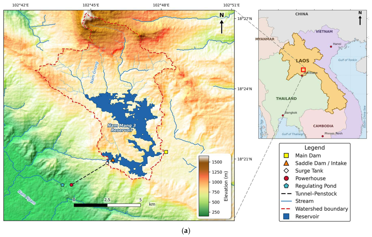
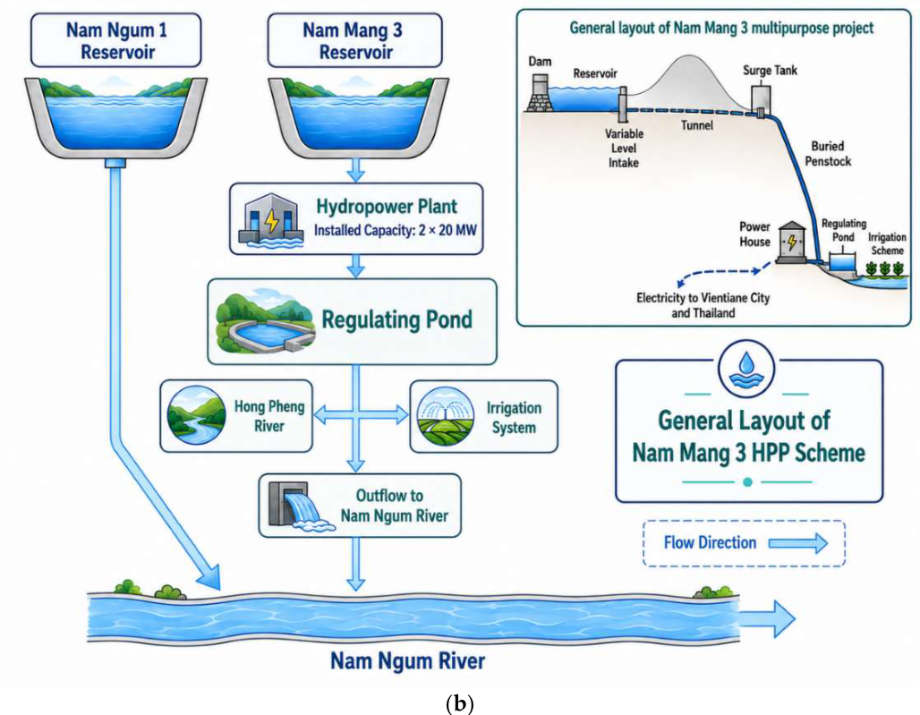
Figure 3.
The six-tool diagnostic protocol. Operating only on the reported results (top row), the mass-balance closure test serves as the shared foundation, and the remaining tools are grouped by the four failure mechanisms (M1−M4); the bottom row summarizes the principal finding of each group.
Figure 3.
The six-tool diagnostic protocol. Operating only on the reported results (top row), the mass-balance closure test serves as the shared foundation, and the remaining tools are grouped by the four failure mechanisms (M1−M4); the bottom row summarizes the principal finding of each group.
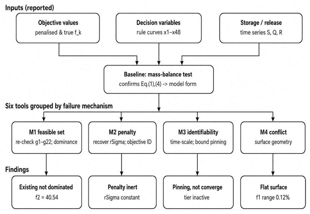
Figure 4.
Overall analytical framework: the reported outputs support the model and formulation reconstruction, explored by the seven algorithms under the diagnostic protocol, leading to the formulation-level findings and the evidence chain in Section 3. No re-running of the model is required.
Figure 4.
Overall analytical framework: the reported outputs support the model and formulation reconstruction, explored by the seven algorithms under the diagnostic protocol, leading to the formulation-level findings and the evidence chain in Section 3. No re-running of the model is required.
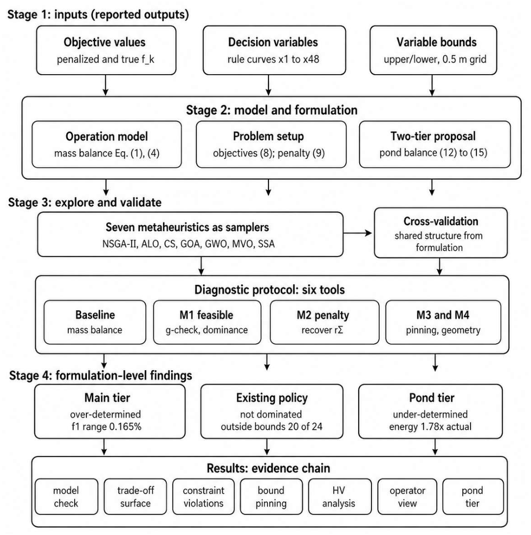
Figure 5.
Water-balance closure of the main reservoir operation. Bars show the beginning-of-month storage; points show the end-of-month storage computed from Equations (1) and (4), which matches the reported value in every month (zero residual); lines on the right axis show the inflow and the release, explaining the direction of the monthly storage change.
Figure 5.
Water-balance closure of the main reservoir operation. Bars show the beginning-of-month storage; points show the end-of-month storage computed from Equations (1) and (4), which matches the reported value in every month (zero residual); lines on the right axis show the inflow and the release, explaining the direction of the monthly storage change.
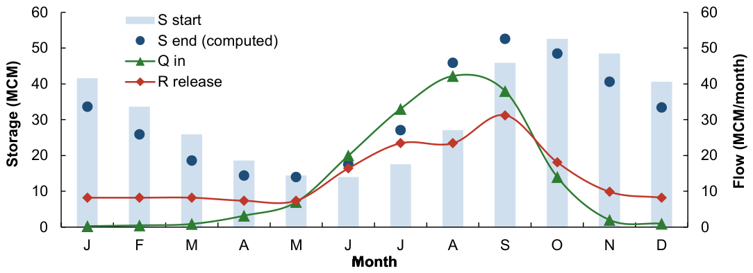
Figure 6.
Structure of the energy and excess-release trade-off from the seven algorithms: (a) the 311-point Pareto front collapses into a nearly vertical line (degenerate surface); (b) the recovered penalty is constant at 23.62 MCM2 (inert penalty); (c) all 35 solutions violate the constraints 5.8−9.2 times more than the existing policy; (d) the existing policy is not dominated in either dimension.
Figure 6.
Structure of the energy and excess-release trade-off from the seven algorithms: (a) the 311-point Pareto front collapses into a nearly vertical line (degenerate surface); (b) the recovered penalty is constant at 23.62 MCM2 (inert penalty); (c) all 35 solutions violate the constraints 5.8−9.2 times more than the existing policy; (d) the existing policy is not dominated in either dimension.
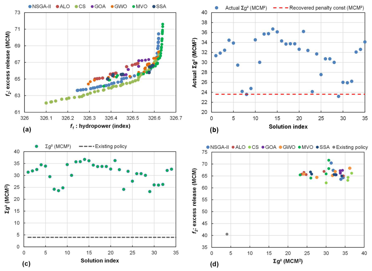
Figure 7.
Mean constraint-violation magnitudes of the seven algorithms for the five violated constraints, in MCM. The constraint g5 at the minimum month is violated identically at 2.78 MCM by every algorithm; the seventeen constraints not shown are never violated in any solution.
Figure 7.
Mean constraint-violation magnitudes of the seven algorithms for the five violated constraints, in MCM. The constraint g5 at the minimum month is violated identically at 2.78 MCM by every algorithm; the seventeen constraints not shown are never violated in any solution.
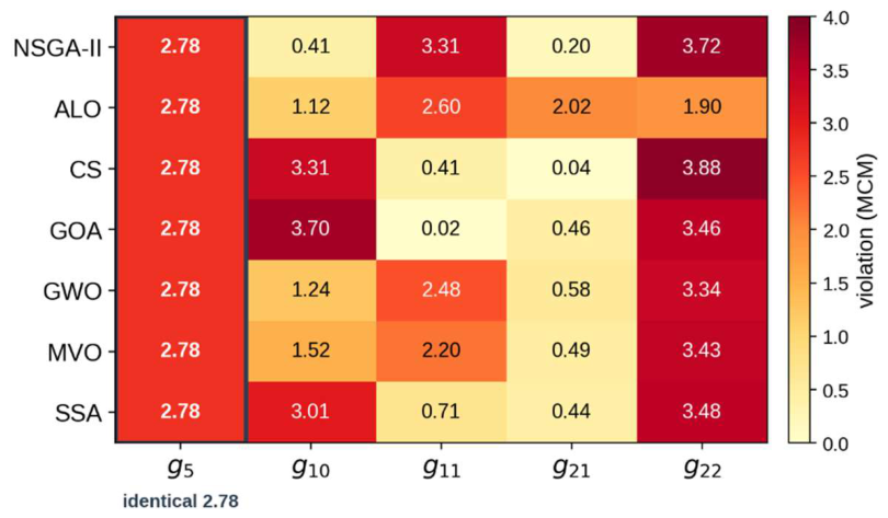
Figure 8.
Temporal deviation of the optimized rule curves from the existing policy, in MCM: (a) the optimized solutions collapse into a single band and deviate clearly after August; (b) the monthly target-storage differences of the lower rule curve peak at approximately 20−22 MCM from August−October, consistent with the year-end constraints.
Figure 8.
Temporal deviation of the optimized rule curves from the existing policy, in MCM: (a) the optimized solutions collapse into a single band and deviate clearly after August; (b) the monthly target-storage differences of the lower rule curve peak at approximately 20−22 MCM from August−October, consistent with the year-end constraints.
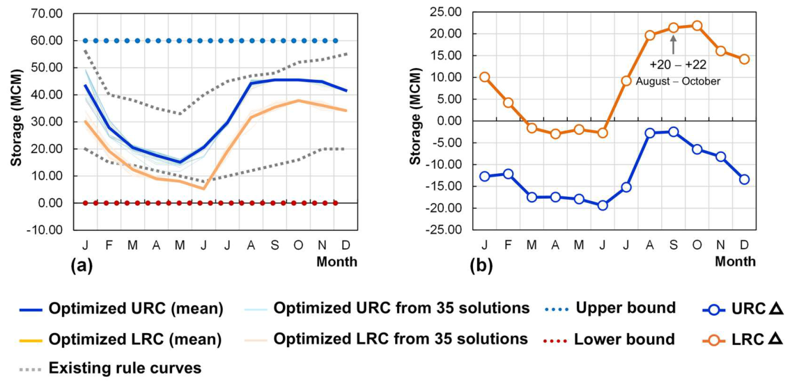
Figure 9.
Rule curves of the seven algorithms at the five Pareto positions RC1−RC5: panels (a)−(g) show the upper rule curves and panels (h)−(n) the lower rule curves, ordered NSGA-II, ALO, CS, GOA, GWO, MVO, and SSA, compared with the existing policy shown as a dashed line, in MCM. The pink band marks the year-end period. In every panel, the curves at the five Pareto positions and across the seven algorithms cluster nearly on top of one another, showing that the deviation is determined by the structure of the problem formulation.
Figure 9.
Rule curves of the seven algorithms at the five Pareto positions RC1−RC5: panels (a)−(g) show the upper rule curves and panels (h)−(n) the lower rule curves, ordered NSGA-II, ALO, CS, GOA, GWO, MVO, and SSA, compared with the existing policy shown as a dashed line, in MCM. The pink band marks the year-end period. In every panel, the curves at the five Pareto positions and across the seven algorithms cluster nearly on top of one another, showing that the deviation is determined by the structure of the problem formulation.
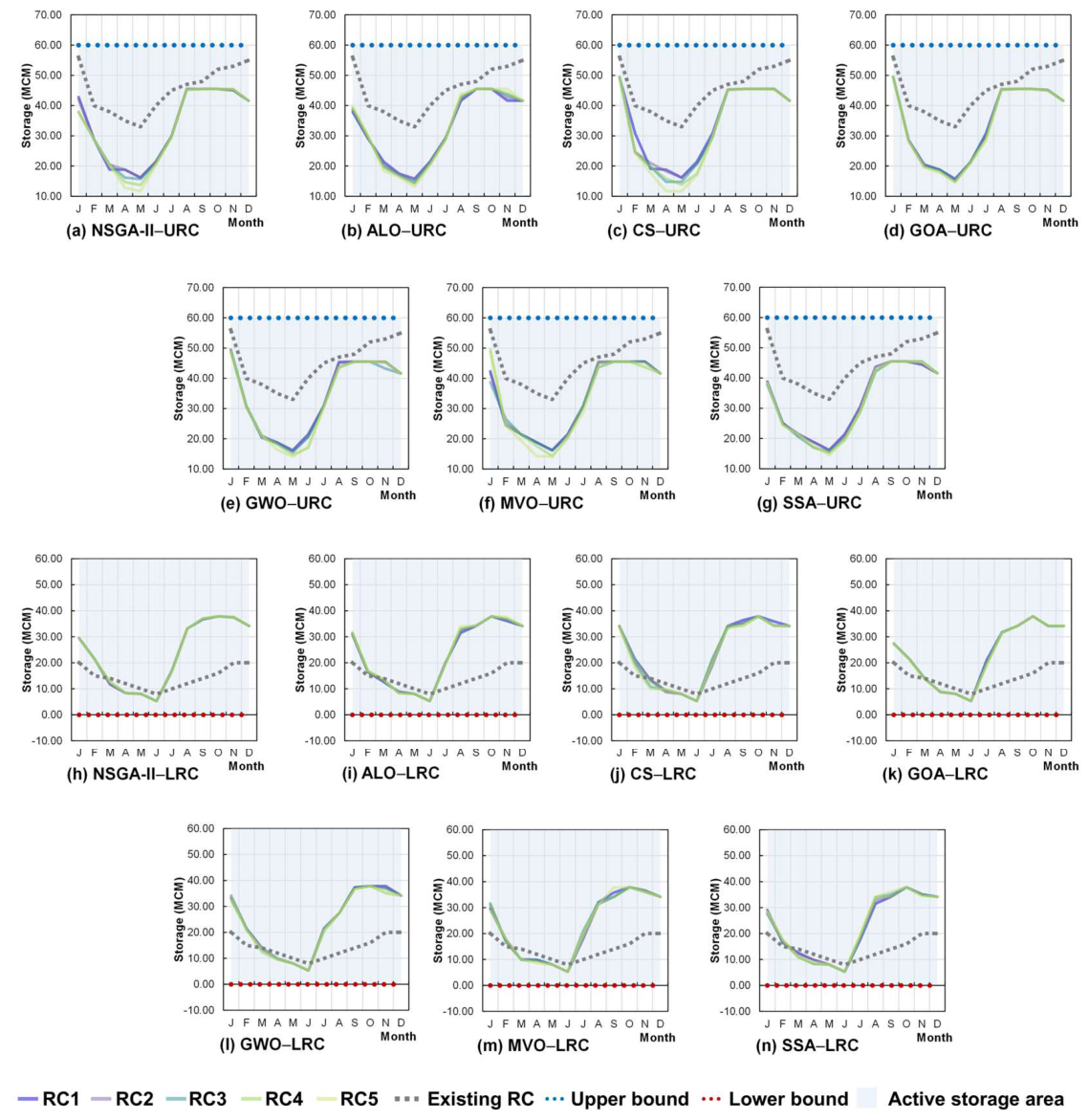
Figure 10.
Monthly variable-bound windows (xU, xL), the 35 representative solutions from the seven algorithms, and the existing rule curves: (a) upper rule curves; (b) lower rule curves. Red circles mark the positions pinned at a bound in every solution.
Figure 10.
Monthly variable-bound windows (xU, xL), the 35 representative solutions from the seven algorithms, and the existing rule curves: (a) upper rule curves; (b) lower rule curves. Red circles mark the positions pinned at a bound in every solution.
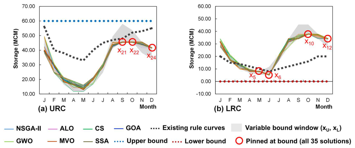
Figure 11.
Annual water-energy accounting of the operating alternatives: (a) annual excess release on the model basis; (b) annual energy from the three data bases; (c) the actual production series and the annual production plan, 2005−2023, with reference levels. Hatched bars are the potential energy equivalents of the excess water by Equation (6).
Figure 11.
Annual water-energy accounting of the operating alternatives: (a) annual excess release on the model basis; (b) annual energy from the three data bases; (c) the actual production series and the annual production plan, 2005−2023, with reference levels. Hatched bars are the potential energy equivalents of the excess water by Equation (6).
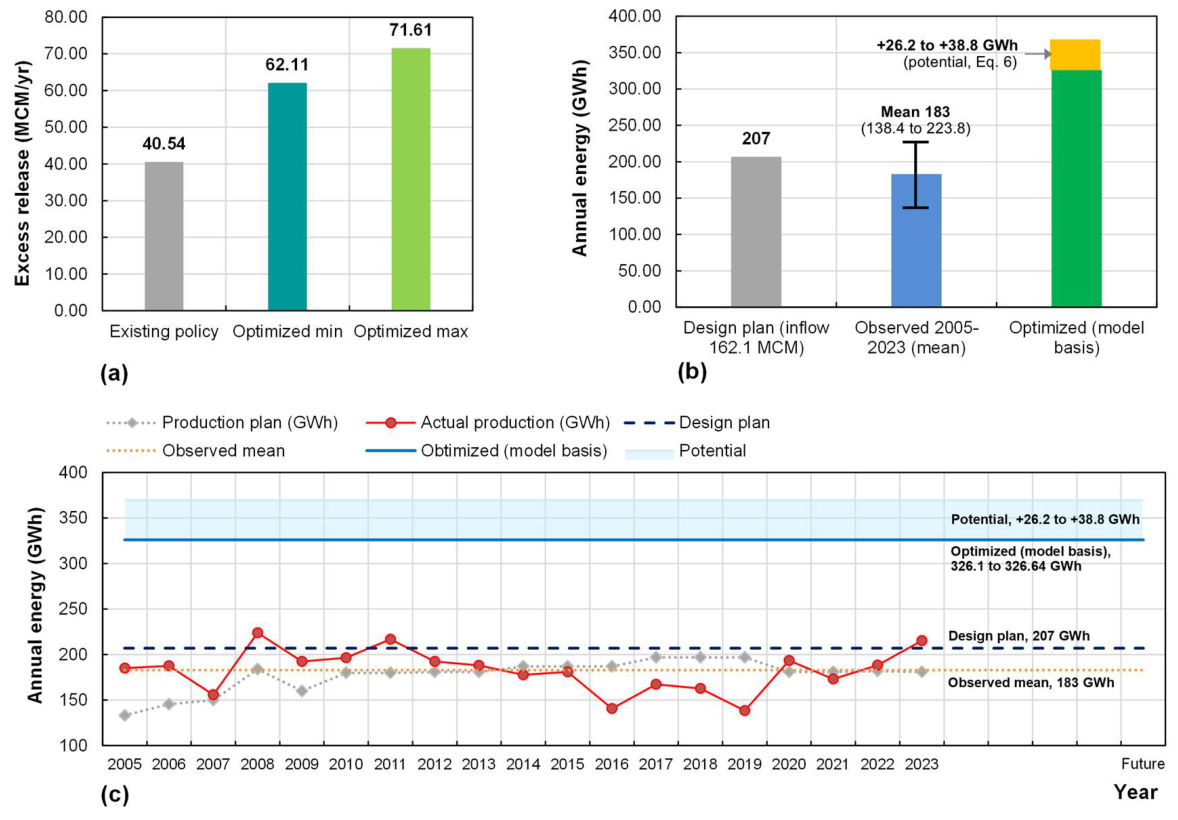
Figure 12.
Rule curves of the regulating pond: the representative solutions RC1−RC5 of each algorithm, compared with the variable-bound windows, which are flat throughout the year (gray bands): (a)−(g) upper rule curves; (h)−(n) lower rule curves.
Figure 12.
Rule curves of the regulating pond: the representative solutions RC1−RC5 of each algorithm, compared with the variable-bound windows, which are flat throughout the year (gray bands): (a)−(g) upper rule curves; (h)−(n) lower rule curves.
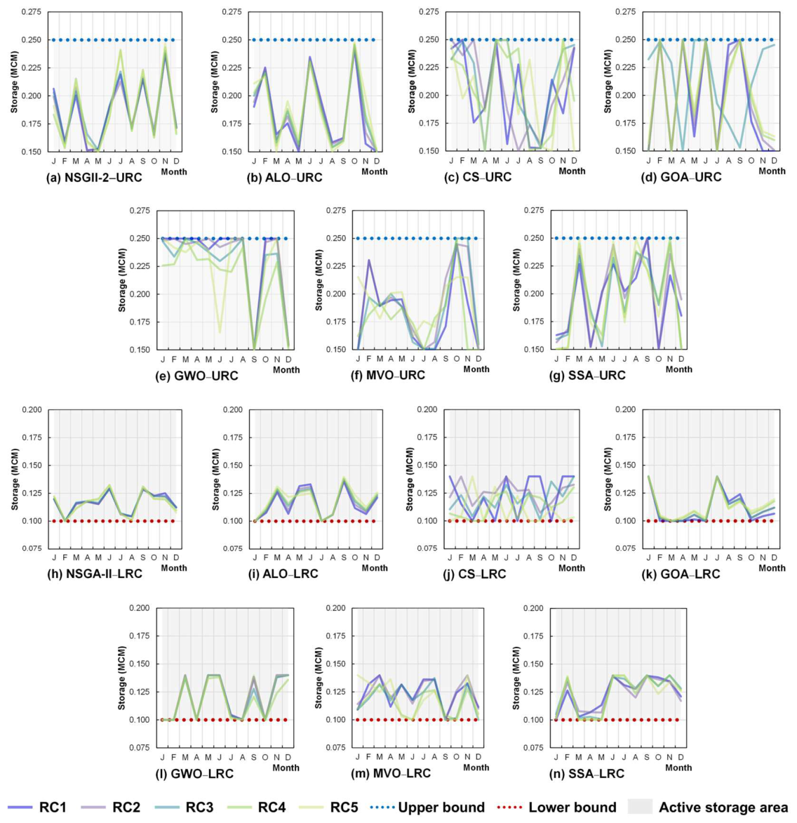
Table 1.
Parameter settings of the seven metaheuristic algorithms.
| No. | Algorithms | Parameters | Values |
|---|---|---|---|
| 1 | Non-dominate sort genetic algorithm-II (NSGA-II) | Probability perform Mutation (Pm) | 0. 1 |
| Probability perform Crossover (Pc) | 0.9 | ||
| Simulated Binary Crossover (SBX) | 0.5 | ||
| 2 | Multi-Objective Ant Lion Optimizer (ALO) |
Stochastic function probability (Pr) | 0.5 |
| Minimum of all variables at t-th iteration (ct) | ct = ct/I | ||
| Maximum of all variables at t-th iteration (dt) | dt = dt/I | ||
| Iteration ratio (I) | I = 1 + 10ω(t/T) | ||
| Omega (ω) | (2,3,4,5,6) | ||
| The current iteration (t) | Iteration count | ||
| The maximum number of iterations (T) | T = Fes/pop size | ||
| 3 | Multi-objective cuckoo search algorithm (CS) | The Levy exponent in Levy flights (β) Discovery probability (Pa) |
1.5 0.25 |
| 4 | Multi-Objective Grasshopper Optimization Algorithm (GOA) | A of decreasing coefficient to shrink the comfort area, repulsion area, and attraction area (c) |
(0.00001,1) |
| 5 | Multi-objective grey wolf optimizer (GWO) | Grid Inflation Parameter (α) | 0.1 |
| Leader Selection Pressure Parameter (β) | 4 | ||
| Extra Repository Member Selection Pressure (γ) | 2 | ||
| Number of Grids per Dimension (Ngrid) | 10 | ||
| 6 | Multi-Objective Multi-Verse Optimizer (MVO) |
Wormhole Existence Probability (WEP) | (0.2,1) |
| Travelling distance rate coefficient | 1/6 | ||
| 7 | Multi-objective Salp Swarm Algorithm (SSA) | balances exploration and exploitation search () | |
| The current iteration (l) | Iteration counting | ||
| The maximum number of iterations (L) | L = Fes / pop size |
Table 3.
Hypervolume statistics of the seven algorithms over repeated runs.
| Algorithms | Mean | std | max | min | Mean - std | Mean + std |
|---|---|---|---|---|---|---|
| NSGA-II | 0.590 | 0.208 | 0.738 | 0.000 | 0.382 | 0.798 |
| ALO | 0.239 | 0.144 | 0.545 | 0.000 | 0.095 | 0.383 |
| CS | 0.600 | 0.277 | 0.805 | 0.000 | 0.322 | 0.877 |
| GOA | 0.075 | 0.154 | 0.574 | 0.000 | −0.079 | 0.229 |
| GWO | 0.310 | 0.232 | 0.679 | 0.000 | 0.078 | 0.543 |
| MVO | 0.649 | 0.126 | 0.721 | 0.000 | 0.524 | 0.775 |
| SSA | 0.340 | 0.124 | 0.633 | 0.141 | 0.216 | 0.464 |
Table 4.
Annual water-energy accounting of the Nam Mang 3 operating alternatives by data basis.
| Data basis / operating alternative | Turbine water (MCM per yr) | Excess release (MCM per yr) | Annual energy (GWh per yr) |
Linked to Figure 11 |
|---|---|---|---|---|
| Design plan, existing policy (inflow 162.1 MCM per yr) |
170.28 | 0 (by plan) | 207 | (b), (c) |
| Actual production, 2005−2023 (19 years) |
150.5ᵃ (113.8−184.1) |
Not recorded | 183.0 (138.4−223.8), averaging 104.4% of the annual production plan | (b), (c) |
| Model, existing policy | Not recordedᵇ | 40.54 | Not recordedᵇ | (a) |
| Model, optimized solutions (lowest to highest) |
268.25−268.69ᵃ | 62.11−71.61 | 326.10−326.64 | (a), (b), (c) |
| Additional excess water as energy equivalent (model basis) | 21.57−31.07 | — | 6.2−37.8 (8.0−11.6% of 326.5; 14.3−20.7% of mean actual production) | (b), (c) |
Notes: ᵃ Computed through the water-use rate w = 0.8226 m3 per kWh of Equation (6); on the design-plan basis, E × w = Qt closes exactly in every month, confirming Equation (6) from an independent source. ᵇ Not recorded by the model. ᶜ The three data bases use different runoff series; energy comparisons are made within the same basis only (see Section 3.8).
Table 5.
Structural indicators of the two-tier problem formulation of the NM3 system.
| Structural indicator | Main reservoir, lower rule curve (x1−x12) |
Main reservoir, upper rule curve (x13−x24) |
Regulating pond, lower rule curve (x25−x36) | Regulating Pond, upper rule curve (x37−x48) |
|---|---|---|---|---|
| Number of decision variables | 12 | 12 | 12 | 12 |
| Number of inequality constraints | 11 | 11 | 0 | 0 |
| Bound-window width (MCM) | 2.78−11.35 | 4.52−12.49 | 0.040 | 0.100 |
| Annual movement of the window midpoint (MCM)ᵃ | 35.05 | 37.81 | 0 | 0 |
| Within-panel solution band relative to window width (%)ᵇ | 4.0−27.2 | 9.5−39.4 | 8.1−90.1 | 9.8−57.4 |
| Values within 2% of a bound (%) | 52.6 | 49.0 | 33.1 | 30.2 |
| Positions pinned in all 35 solutions (of 12)ᶜ | 4 | 3 | 0 | 0 |
| Mean reversals per curve (per year) | 2.00 | 2.00 | 6.60 | 6.69 |
| Mass-balance equations | (1), (4) | (1), (4) | — | — |
Notes: ᵃ A value of 0.00 means the bound window is constant throughout the year, with no seasonal structure. ᵇ Monthly mean of the RC1−RC5 band within a panel divided by the window width, showing the range across the seven algorithms (Figure 9 and Figure 12). ᶜ Main reservoir: x5, x6, x10, x12 (lower rule curve) and x21, x22, x24 (upper rule curve), per Figure 10.
Disclaimer/Publisher’s Note: The statements, opinions and data contained in all publications are solely those of the individual author(s) and contributor(s) and not of MDPI and/or the editor(s). MDPI and/or the editor(s) disclaim responsibility for any injury to people or property resulting from any ideas, methods, instructions or products referred to in the content. |
© 2026 by the authors. Licensee MDPI, Basel, Switzerland. This article is an open access article distributed under the terms and conditions of the Creative Commons Attribution (CC BY) license (http://creativecommons.org/licenses/by/4.0/).
Copyright: This open access article is published under a Creative Commons CC BY 4.0 license, which permit the free download, distribution, and reuse, provided that the author and preprint are cited in any reuse.