

Submitted:
02 September 2026
Posted:
02 September 2026
You are already at the latest version
Abstract
Accurate representation of frequency-dependent cable parameters is essential for evaluating power losses and voltage regulation in medium-voltage wind-farm collection networks. This paper develops a MATLAB-based electromagnetic framework using frequency-dependent series-impedance (Z) and shunt-admittance (Y) matrices for underground cables, including conductor skin and proximity effects and earth-return impedance. Four earth-return formulations—Saad–Gaba–Giroux, Wedepohl series, Wedepohl, and infinite-earth—are implemented and benchmarked against RSCAD over the frequency range from 10 Hz to 1 MHz. The validated model is applied to a wind-farm collection system in the Isthmus of Tehuantepec, Oaxaca, Mexico, comprising five 1.5 MW wind turbines connected at 13.8 kV through two radial underground circuits. The results show that the Saad–Gaba–Giroux and Wedepohl-series formulations provide the closest agreement with the RSCAD reference. At a power factor of 0.9, the conventional constant core-resistance model underestimates the modeled active-power loss by up to 60% under the evaluated operating conditions. The frequency-dependent model also predicts voltage drops of 0.68% and 1.55% for Circuits 1 and 2, respectively, whereas the simplified DC representation predicts values below 0.15%. A component-level analysis identifies the core conductor as the dominant contributor to active-power dissipation, while the earth-return path has a significant influence on the equivalent phase resistance and voltage-drop behavior. These results demonstrate that frequency-dependent cable modeling can provide a more comprehensive basis for technical assessment and techno-economic evaluation of medium-voltage wind-farm collection systems.
Keywords:
frequency-dependent cable parameters
; underground cables
; wind-farm collection networks
; earth-return impedance
; power losses
; voltage drop
; RSCAD
; techno-economic planning
1. Introduction
Wind energy has become a major source of utility-scale renewable electricity. However, the electrical collection system remains a critical component of wind-farm planning because conductor losses, voltage regulation, installation constraints, and environmental conditions directly affect technical performance and project economics. The case study considered in this work is located in the Isthmus of Tehuantepec, Oaxaca, Mexico, a region with substantial wind-energy potential. The proposed design comprises five 1.5 MW wind turbines, corresponding to a nominal installed capacity of 7.5 MW, connected through a 13.8 kV medium-voltage underground collection network. Accurate representation of the collection cables is therefore important for assessing the electrical behavior of the proposed infrastructure [1,2,3].
In preliminary design, cable losses and voltage drop are often estimated using a constant direct-current (DC) resistance. This simplification is attractive because of its low computational cost; however, it does not account for the frequency dependence of conductor impedance associated with skin and proximity effects, nor does it fully represent the contribution of the earth-return path. These effects modify the series impedance of the cable system and may become relevant when cable geometry, conductor arrangement, grounding conditions, and operating conditions are considered simultaneously [4,5,6,7].
A more comprehensive representation is obtained from the multiconductor Telegrapher equations using frequency-dependent series-impedance (Z) and shunt-admittance (Y) matrices. A key analytical challenge is the evaluation of Pollaczek-type earth-return integrals, for which several approximations have been proposed, including the Saad–Gaba–Giroux, Wedepohl, Semlyen, and infinite-earth formulations [7,8,9,10]. Although these formulations are individually well established, their comparative effects on the predicted cable parameters and, consequently, on wind-farm power losses and voltage regulation have not been sufficiently characterized for the case-study configuration considered in this work.
Accordingly, this paper develops a MATLAB-based frequency-dependent cable model and validates four earth-return formulations against RSCAD over the frequency range from 10 Hz to 1 MHz. The validated model is subsequently applied to the two radial collection circuits of the 7.5 MW case study. The main contributions of this work are as follows: (i) implementation of a unified (ZY) framework that incorporates conductor, insulation, sheath, and earth-return effects; (ii) quantitative comparison of four earth-return approximations against an RSCAD benchmark; (iii) evaluation of their effects on active-power losses and voltage drop under different power-factor conditions; and (iv) a techno-economic interpretation that identifies the additional information required to translate operating-point electrical-loss differences into annual energy and economic impacts. The results provide a basis for determining when a simplified DC representation may be insufficient for medium-voltage wind-farm collection-system planning.
2. Electromagnetic Modeling of Underground Cables
The quasi-transverse electromagnetic (quasi-TEM) propagation along the longitudinal axis of the cable system is described by the multiconductor Telegrapher equations in the phase domain:
where V and I are voltage and current vectors, and Z and Y are, the frequency dependent series impedance and shunt admittance per unit length, respectively.
2.1. Underground Cable System Infrastructure
Medium-voltage underground collection networks may operate at different voltage levels depending on the wind-farm configuration and grid requirements. In the present case study, the collection system operates at 13.8 kV. As shown in Figure 1, the system comprises three single-phase coaxial cables buried at the same depth and arranged in a flat configuration. Each cable consists of two concentric metallic conductors, namely the core and sheath, surrounded by two insulating layers.
The electromagnetic parameters of the cable system are determined from the conductor geometry, material properties, cable spacing, burial depth, and surrounding soil characteristics. These parameters are subsequently incorporated into the primitive impedance and admittance matrices used to obtain the equivalent three-phase frequency-dependent cable model.
2.2. Conductor Impedance
The formulation accounts for the frequency-dependent internal impedance of the conductor through modified Bessel functions. (I0) and (I1) denote modified Bessel functions of the first kind of orders zero and one, respectively, whereas (K0) and (K1) denote modified Bessel functions of the second kind of orders zero and one, respectively.
2.3 Insulator impedance
The impedance associated with each insulation layer is calculated according to [4]:
where µ0=4πx10-7 H/m is the permeability of free space, and ri and ro are the inner and outer radii of the corresponding insulation layer, respectively. The electromagnetic parameters of each dielectric layer are evaluated according to its material properties and boundary radii, as illustrated in Figure 1.
2.3. Impedance of Tubular Conductors
The internal, external, and mutual impedances of the tubular conductors are calculated according to [5]:
with
These formulations account for the electromagnetic behavior of the metallic sheath and its coupling with the other conductors of the cable system.
2.4. Earth-Return Impedances
The self and mutual impedances associated with the earth-return path are calculated according to [4,7]:
where Js and Jm represent the Pollaczek integrals associated with the self and mutual earth-return impedances, respectively [4,7].
The Pollaczek integral (Js) is expressed as:
where (h) is the cable burial depth, (R) is the outer cable radius, and the remaining variables are defined according to the cable geometry shown in Figure 2. is the wave number.
The corresponding mutual earth-return formulation is obtained from the same general expression by considering the burial depths of the two cables and their horizontal separation. The geometrical variables R, d, h, and D used in the earth-return formulations are illustrated in Figure 2.
2.5. Loop-to-Conductor Quantity Transformation
To perform system-level power-loss and voltage-drop calculations, the loop quantities (LQ) used in the initial formulation are transformed into physical conductor quantities (CQ) through linear matrix transformations [4,5]:
For a single-phase coaxial cable comprising a core and a sheath, the corresponding transformation matrices are defined as:
These transformations allow the electromagnetic quantities calculated in loop coordinates to be expressed in terms of the physical conductors of the cable. This representation is subsequently used to assemble the conductor-quantity impedance and admittance matrices required for the three-phase cable model.
2.6. Parallel Admittance Matrix Formulations
The primitive shunt-admittance matrix per unit length, YCQ, for a single coaxial cable is assembled in conductor coordinates as a diagonal matrix representing the dielectric properties of the individual insulation layers [4]:
The capacitance per unit length, Ci, and conductance per unit length, Gi, associated with each concentric dielectric layer are calculated from the corresponding boundary radii and dielectric loss factor tanδ. The angular frequency is ω=2πf. The capacitance per unit length is given by
where ε0 is the vacuum permittivity, εri is the relative permittivity of the i-th insulation layer, and ri and ro are the inner and outer radii of the corresponding dielectric layer, respectively. In the present model, dielectric losses in the insulation layers are neglected. Therefore, the corresponding shunt conductance is set to zero Gi=0.
The resulting dielectric admittances are then assembled to form the primitive shunt-admittance matrix of the cable. This matrix is subsequently incorporated into the three-phase cable representation together with the frequency-dependent series-impedance matrix.
2.7. Matrix Assembly and Kron Reduction
For the three-phase system comprising three parallel cables, the primitive series-impedance matrix (Zs) and shunt-admittance matrix (Yp) are assembled using the corresponding self and mutual cable blocks. The diagonal blocks of Zs correspond to the conductor-quantity impedance matrix ZCQ, whereas the off-diagonal blocks include the mutual earth-return impedance contributions Zem,ij. The off-diagonal blocks of Yp are zero matrices of appropriate dimensions.
Under the solid-grounding condition, the sheath voltages are assumed to be zero, i.e., Vsh=0. Accordingly, the series-impedance and potential matrices are partitioned into core and sheath variables, and Kron reduction is applied to eliminate the sheath variables [7,8]:
where the subscripts (c) and (sh) denote the core and sheath variables, respectively. The resulting reduced matrix represents the equivalent electrical behavior of the three active phase conductors after eliminating the internal sheath variables. The reduced frequency-dependent matrices are subsequently used in the cable-network calculations for the evaluation of currents, voltage drop, and power losses.
The corresponding equivalent admittance matrix is obtained from the reduced formulation as Yabc = Pabc-1 where Yabc represents the equivalent three-phase shunt-admittance matrix in phase coordinates.
3. Earth Return Impedance Approximations
Several analytical approaches have been reported for the evaluation of earth- and sea-return impedances in underground power cables [21]. In this study, four formulations are considered for the evaluation of the earth-return impedance (Ze): the Saad–Gaba–Giroux (SGG) formulation, the Wedepohl-series (WS) formulation, the Wedepohl (WE) formulation, and the infinite-earth (IE) formulation [7,8]. Although the formulations differ in their mathematical treatment of the earth-return contribution, all four are used to obtain the corresponding frequency-dependent (Ze).
The resulting Ze values are incorporated into the cable series-impedance matrix and subsequently evaluated over the frequency range from 10 Hz to 1 MHz. The four formulations are compared with the RSCAD reference model in Section 5 to assess their accuracy in reproducing the frequency-dependent cable parameters.
3.1. Saad-Gaba-Giroux Formulas
The Saad–Gaba–Giroux (SGG) formulas provide closed-form approximations for evaluating the self and mutual earth-return impedance components of underground cables [9]. These formulas are derived to avoid the direct numerical evaluation of the Pollaczek integral, which constitutes a component of the earth-return impedance formulation.
The SGG formulas for the self and mutual earth-return impedance terms are expressed as follows [9]:
where l=hi+hj, and the geometrical variables R, d, h, and D are defined according to the cable geometry shown in Figure 2.
The resulting self and mutual earth-return impedance components are incorporated into the total series-impedance formulation (Zs) of the cable system. The SGG formulation is subsequently evaluated over the frequency range from 10 Hz to 1 MHz and compared with the RSCAD reference results in Section 5.
3.2. Wedepohl and Wilcox Formulas
The formulas proposed by Wedepohl and Wilcox [8] for evaluating self and mutual impedances in underground cables are
where γ=0.57721 and l=hi+hj. The parameters are defined according to the cable geometry, conductor properties, burial depth, conductor spacing, and soil characteristics introduced in Section 2.
The resulting impedance terms are incorporated into the total series impedance (Zs) of the cable system [8].
3.3. Wedepohl Formula
3.4. Semlyen Formula
Semlyen proposed the following formulation for calculating the self earth-return impedance of underground cables [4]:
This formulation is included for completeness but is not considered among the four formulations selected for the RSCAD comparative validation.
3.5. Infinite Earth-Return Model
For an idealized infinite earth-return path, the self and mutual earth-return impedances can be expressed using the formulation reported in [4]. The corresponding expressions are given by
and
where the parameters defining the conductor geometry and earth-return path are consistent with those introduced in Section 2.
This formulation represents the ideal infinite-earth approximation and is used as a reference case for comparison with the analytical and numerical formulations considered in the following sections.
3.6. Numerical Integration and Series Solution
The Pollaczeck integral in (12) can be evaluated using the analytical decomposition proposed by Wedepohl and Wilcox in [8]. Accordingly, the integral term (J) is expressed as
where IWW denotes the definite integral introduced by Wedepohl and Wilcox, given by
For the mutual earth-return impedance (Jm), the parameters are defined as h=(hi+hj)/2 and t=2h/D, whereas for the self-earth-return impedance (Js), h=hi and x=R. The remaining geometrical parameters are defined according to the cable configuration presented in Section 2.
The integral IWW does not generally accept a closed-form analytical solution and is therefore evaluated by numerical integration. This approach provides a direct numerical reference for the evaluation of the earth-return contribution to the cable impedance.
Alternatively, the integral IWW can be evaluated using the recursive series solution reported in [12,13,22], expressed as
with
The numerical integration and recursive series approaches provide two equivalent procedures for evaluating the same earth-return integral. Their comparison is subsequently used to assess the numerical consistency of the impedance calculations.
4. Wind Farm Design Data
This section briefly describes the wind resource and the technical data of the wind turbine selected for the design of a large-scale wind farm. The study is localized at the Universidad del Istmo (UNISTMO), Juchitán Campus, within the Isthmus of Tehuantepec, Oaxaca, Mexico—a region characterized by exceptionally high wind energy density [1].
4.1. Wind Resource
An empirical case study was conducted using micrometeorological data from the Regional Center for Wind Technology (CERTE) at La Ventosa station, Oaxaca, Mexico (31 masl), located 1.3 km from the projected site. The station uses Class-1 instrumentation and follows WMO guidelines for wind measurements [14], while the wind-turbine power-performance assessment follows IEC 61400-12-1 requirements [15]. The database analyzed comprises continuous wind-speed and wind-direction measurements recorded at 10-min intervals over a 12-month period. Wind-speed measurements were available at vertical heights of 20, 40, 60, and 80 m, while the wind-direction measurements used for the directional analysis were recorded at 78 m.
The wind-speed analysis presented in this study corresponds to the measurements at 80 m. The wind-speed histogram (Figure 3) therefore represents the 80 m measurement height, and the corresponding Weibull fitting parameters are reported in Table III. In contrast, the directional analysis was performed using the wind-direction measurements at 78 m. As shown in Figure 4, the annual wind rose indicates a strong predominance of winds from the north-northwest (NNW) direction. The NNW-related directional range accounts for 63.7% of the total samples, while the remaining directions account for 36.3%, as summarized in Table II.
Furthermore, the wind-speed histogram (Figure 3) reveals an operational velocity spectrum of 0 ≤ Vw ≤32 m/s. This frequency distribution is fitted using both unimodal and bimodal Weibull probability density functions to characterize the localized wind-speed distribution.
The standard unimodal Weibull distribution is expressed as:
where Vw is the wind speed (m/s), while k and c denote the dimensionless shape and scale (m/s) parameters, respectively. To accurately capture the multi-regime wind behavior of the site, a bimodal Weibull PDF is implemented by combining two independent unimodal functions as follows [15]:
where p represents the weighting factor associated with the sample distribution of each operational mode (0 ≤p ≤1).

Table I.
Wind Database CERTE.
| General Data | |||
| Location | La Ventosa | Altitude | 31 masl |
| Latitude | 16° 32′ 49.27″ N | Longitude | 94° 57′ 20.83″ W |
| Start date |
Jan 01/2018 00:00 | End date |
Dec 31/2018 23:59 |
| Duration | 12 months | Wind class | 7 (Excellent) |
Table II.
Annual Wind Rose Data at 78 Meters Height.
| Directions (°) | Sectors | Frequency (%) |
| 330°–340° | NNW | 30.4 |
| 330°–350° | NNW | 22.5 |
| 350°–360° | NNW-N | 10.8 |
| 330°–360° | NNW | 63.7 |
| 0° to <330° | Between N and WNW | 36.3 |
Note: NNW-related directional range spans 330°–360°, while the remaining directional range spans 0° to <330°. The reported frequencies correspond to the directional groupings used in the wind-resource analysis.
Table III.
Fitting Wind Speeds with Weibull Function at 80 Meters Height.
| Method | k | c (m/s) | RMSE |
| MLE | k₁ = 1.809 | c₁ = 10.522 | 0.0039 |
| JUSTUS | k₁ = 1.835 | c₁ = 10.531 | 0.0041 |
| EPFM | k₁ = 1.838 | c₁ = 10.531 | 0.0042 |
| MOM | k₁ = 1.825 | c₁ = 10.399 | 0.0041 |
| Bimodal | k₁ = 1.621, k₂ = 2.684 | c₁ = 7.282, c₂ = 13.683 | 0.0026 |
Table III summarizes the parameters obtained through different analytical fitting methods [14,16]. The statistical analysis demonstrates that the bimodal formulation achieves the optimal fit with a minimum root-mean-square error (RMSE) of 0.0026. As depicted in Figure 4, this optimal distribution is characterized by scale factors of c1 = 7.282 m/s and c2=13.683 m/s, coupled with shape factors of k1 = 1.621 e k2 = 2.684.
4.2. Wind Turbine
The generation infrastructure utilizes the Acciona AW-1500/70 wind turbine generator. The main technical specifications are summarized in Table IV. As illustrated by the manufacturer power curve in Figure 5, the rated power of 1500 kW is achieved at a nominal wind speed of 11.6 m/s. Under the IEC 61400-1 standard framework, this turbine is designated as Class IA, with a reference wind speed of Vref = 50 m/s and a reference turbulence intensity of I = 0.16 [2]. Wind-speed fluctuations are modeled using the standard deviation (σ₁) of the Normal Turbulence Model (NTM), defined as:
where Vhub represents the wind speed at hub height and c= 5.6 m/s is a constant parameter. The rated terminal voltage of VLL= 13.8 kV and the grid operating frequency of f = 60 Hz are used as the electrical operating conditions for the proposed wind-farm collection system. Table IV summarizes the technical specifications of the Acciona AW-1500/70 wind turbine.
The comprehensive wind-farm layout, comprising five identical AW-1500/70 units, is depicted in Figure 6. To optimize the micro siting configuration, collection-network routing, and turbine spacing while limiting wake-related energy losses and structural loading, the turbine arrangement follows the spacing criteria adopted in the wind-farm design.
The crosswind spacing is fixed at 483.1 m, corresponding to 6.9 times the rotor diameter (D), whereas the downwind longitudinal spacing is set to 8.0D. Micro siting optimization performed using WAsP software [18] estimates a Gross Annual Energy Production (GAEP) of 29.67 GWh. Considering an estimated wake attenuation loss of 4%, the corresponding Net Annual Energy Production (NAEP) is calculated as 28.48 GWh/year.
The NAEP value is obtained according to:
where Lwake is the wake-loss fraction. For GAEP = 29.67 GWh and Lwake = 0.04, the resulting value is approximately 28.48 GWh/year.
4.3. Underground Cable System
The medium-voltage underground collection infrastructure comprises two main radial circuits, whose spatial arrangement is shown in Figure 6 and whose technical specifications are detailed in Table V. The nominal operating current (In) of each wind turbine generator is evaluated as follows:
where Pn = 1500 kW is the rated turbine power, VLL = 13.8 kV is the RMS line-to-line terminal voltage, and cos(φ)= 0.9 is the baseline operating power factor. This yields an individual turbine rated current of In = 69.72 A. Consequently, the operating current requirements for Circuit 1, comprising two turbines, and Circuit 2, comprising three turbines, are In,C1=139.5 A and In,C2=209.2 A, respectively, resulting in a total wind-farm collection current of IT=348.7 A. Conductor sizing incorporates a continuous safety overload margin factor of Fs=1.2.
The geometric properties, cross-sectional layer parameters, and electromagnetic boundaries of the three-phase underground cable system are illustrated in Figure 7 and summarized in Table VI. The cable cross-sectional geometry is described using the radial boundaries r1, r2, r3, and r4, as illustrated in Figure 7. These radial parameters define the geometric boundaries used in the frequency-dependent cable-parameter calculations. The same geometric definitions are maintained throughout the electromagnetic model to ensure consistency between the cable construction data and the calculated series impedance and shunt admittance. The cable network is buried at a standard depth of hi = 1.1 m, with a flat-formation phase separation of x= 0.25 m, embedded within a homogeneous soil medium with a constant ground resistivity of ρsoil= 100 Ω-m. The technical parameters of the two cable configurations used in the collection circuits are summarized in Table VI.
5. Model Validation
Although the wind-farm collection system operates at the fundamental grid frequency of 60 Hz, the proposed model was validated over the broader frequency range from 10 Hz to 1 MHz to assess its frequency-dependent electromagnetic behavior and the accuracy of the implemented earth-return formulations beyond the fundamental operating frequency. The subsequent steady-state analysis of the wind-farm collection circuits is performed at the 60 Hz operating frequency, whereas the extended frequency-domain validation is used to verify the general consistency of the cable model and its earth-return formulations [11]. RSCAD was used as the reference benchmark to assess the general consistency of the cable model [11].
RSCAD was used as the reference benchmark to evaluate four earth-return formulations implemented in MATLAB: the Saad-Gaba-Giroux (Zse,sgg), the Wedepohl-series (Zse,ws), the Wedepohl formulation (Zse,we), and the infinite earth-return (Zse,ei).
The agreement between the MATLAB and RSCAD results was quantified using the root-mean-square error (RMSE), defined as:
where N is the number of frequency points, is the value obtained from the proposed MATLAB model, and is the corresponding reference value obtained from RSCAD. The RMSE was calculated over the evaluated frequency range for each electrical parameter and earth-return formulation.
5.1. Resistance
Figure 8 and Figure 9 illustrate the frequency responses of the self-resistance (Rs,11) and mutual resistance (Rm,12), respectively, for the 1/0 AWG cable of Circuit 1. For Rs,11, shown in Figure 8, all formulations exhibit a monotonic increase with frequency, consistent with the expected influence of the skin effect. The MATLAB-based results show close agreement with the RSCAD reference over the entire frequency range.
Over the evaluated frequency range from 10 Hz to 1 MHz, the Saad–Gaba–Giroux (Zse,sgg) and Wedepohl-series (Zse,ws) formulations provide the closest agreement with the RSCAD reference, yielding an RMSE of 1.53×10⁻⁵. In contrast, the Wedepohl (Zse,we)and infinite-earth (Zse,ei)formulations exhibit slightly larger deviations, with an RMSE of 1.69x10⁻⁵.
For the mutual resistance Rm,12, shown in Figure 9, the response is concentrated primarily in the 10 Hz–100 Hz range and decreases rapidly with increasing frequency, becoming negligible above approximately 1 kHz. Within the low-frequency range, the Saad-Gaba-Giroux and Wedepohl formulations closely reproduce the peak observed in the RSCAD reference, yielding a minimum RMSE of 1.18x10⁻⁷. In contrast, the Wedepohl formulation underestimates the peak magnitude, whereas the infinite-earth formulation (Zse,ei) exhibits the largest deviation, with an RMSE of 1.32x10⁻⁵.
5.2. Inductance
Figure 10 and Figure 11 illustrate the frequency responses of the self-inductance (Ls,11) and mutual inductance (Lm,12), respectively, over the frequency range from 10 Hz to 1 MHz. For Ls,11, shown in Figure 10, a nonlinear decrease is observed between 10 Hz and approximately 100 Hz, which can be attributed to the frequency-dependent effects of skin and proximity. Above 1 kHz, the response gradually stabilizes and approaches an asymptotic minimum of approximately 0.15 mH/m. The MATLAB-based formulations show close agreement with the RSCAD benchmark over the medium- and high-frequency ranges, with only minor deviations at 10 Hz for the infinite-earth (Zse,ei) model. Among the evaluated formulations, the Saad-Gaba-Giroux (Zse,sgg) and Wedepohl-series (Zse,ws) formulations provide the closest agreement with the RSCAD results, yielding RMS values of 1.28x10⁻⁸ and 2.45x10⁻⁸, respectively.
Conversely, the Lm,12 profiles shown in Figure 11 exhibit a continuous decrease in magnitude with increasing frequency, approaching zero at high frequencies. In the 10 Hz–1 kHz range, noticeable differences among the formulations can be observed. The Saad-Gaba-Giroux and Wedepohl-series formulations closely reproduce the magnetic coupling behavior predicted by RSCAD, with an RMSE of 1.92x10⁻⁵. In contrast, the Wedepohl and infinite-earth formulations underestimate the magnitude of the mutual inductance, with the infinite-earth formulation exhibiting the largest deviation, with an RMSE of 1.921x10⁻⁵.
5.3. Capacitance
Figure 12 illustrates the frequency response of the self-capacitance (C11) from 10 Hz to 1 MHz for the wind-farm collection system. In the low-frequency range (10 Hz–1 kHz), small variations in the calculated self-capacitance are observed. Above 1 kHz, the response gradually stabilizes and remains approximately constant over the remaining frequency range up to 1 MHz. Above 1 kHz, the response gradually stabilizes and approaches an asymptotic behavior over the remaining frequency range up to 1 MHz. The results obtained with the proposed MATLAB algorithm show close agreement with the RSCAD benchmark, confirming the accuracy and consistency of the proposed methodology for estimating the cable capacitance per unit length.
6. Power Losses and Voltage Drop Analysis
This section evaluates the percentage active power losses and voltage drop in the two medium-voltage collection circuits. The frequency-dependent (ZY) formulation is compared with the conventional constant core-resistance model (RDC,core) over power factors (pf) ranging from 0.5 to 1.0. The objective is to determine whether the simplified representation adequately captures the electrical performance of the collection system and the differences identified by the frequency-dependent cable model. For the wind-farm operating-point analysis, the frequency-dependent cable parameters are evaluated at the fundamental system frequency of 60 Hz.
The percentage voltage drop is calculated from the sending-end and receiving-end voltage magnitudes according to:
where Vs and Vr are the sending-end and receiving-end voltage magnitudes, respectively.
For the proposed ZY model, the sending-end and receiving-end voltages are obtained from the frequency-dependent series-impedance and shunt-admittance matrices evaluated at 60 Hz. The calculation therefore accounts for the conductor, metallic sheath, insulation, mutual coupling, and earth-return effects represented in the reduced three-phase cable model.
The percentage active power losses and voltage-drop profiles are evaluated as functions of the power factor. As illustrated in Figure 13, both steady-state performance indicators are plotted over the range from pf = 0.5 to 1.0, comparing the (ZY) cable model with the (RDC,core) representation.
Regarding the percentage power losses (PLoss) in Figure 13a, a nonlinear monotonic decrease is observed as the power factor approaches unity, primarily because the current magnitude decreases as the reactive-power component is reduced. The complete (ZY) model, represented by dashed lines, predicts consistently higher losses than the (RDC,core) formulation, represented by solid lines. At pf = 0.5, the ZY model predicts a maximum loss of 0.26% for Circuit 2, whereas the DC-based representation predicts approximately 0.15%. This difference reflects the limitations of a constant-resistance representation in capturing the frequency-dependent behavior of the cable impedance.
At pf = 0.9, (RDC,core) predicts a loss of 0.03% for Circuit 1, compared with 0.04% obtained with the comprehensive (ZY) model. Across the evaluated operating conditions and circuits, the maximum relative underestimation of active power losses by the simplified DC representation is approximately 60%.
In contrast, the percentage voltage-drop (ΔV) profiles in Figure 15b exhibit a more pronounced divergence between the two formulations. With the (RDC,core) representation, the voltage drop remains below 0.25% over the evaluated power-factor range. The complete ZY model predicts higher voltage-drop values because it incorporates the frequency-dependent series impedance together with conductor coupling and earth-return effects.
At pf = 0.5, the maximum voltage drop predicted for Circuit 1 is 1.15%. At the reference operating condition of pf = 0.9, the simplified DC model predicts voltage drops below 0.15% for both circuits, whereas the complete ZY model predicts approximately 0.68% and 1.55% for Circuits 1 and 2, respectively. These results demonstrate that the use of simplified DC parameters can significantly underestimate voltage-drop behavior in medium-voltage underground collection systems.
6.1. Breakdown of Percentage Power Losses
Figure 14 presents the percentage power losses as a function of power factor from 0.5 to 1.0, separating the individual contributions of the core conductor, metallic sheath, and earth-return path. For Circuit 1 (C1).
For Circuit 1, the highest component-level losses are observed at pf=0.5. At pf=0.5, the maximum losses are observed, with the core conductor contributing 0.0851%, followed by the earth-return path at 0.0430% and the metallic sheath at 0.0014%. At (pf=0.9), these contributions decrease to 0.0261%, 0.0132%, and 0.0004%, respectively. At unity power factor, the corresponding minimum values are 0.0212% for the core conductor, 0.0107% for the earth-return path, and 0.0003% for the metallic sheath.
Across the evaluated operating conditions, the core conductor remains the dominant contributor to active-power dissipation, followed by the earth-return path and the metallic sheath. This decomposition indicates that the active-power losses are primarily associated with the core conductor, while the earth-return path represents a secondary but non-negligible contribution to the total loss.
Figure 14.
Percentage power losses for circuit 1.
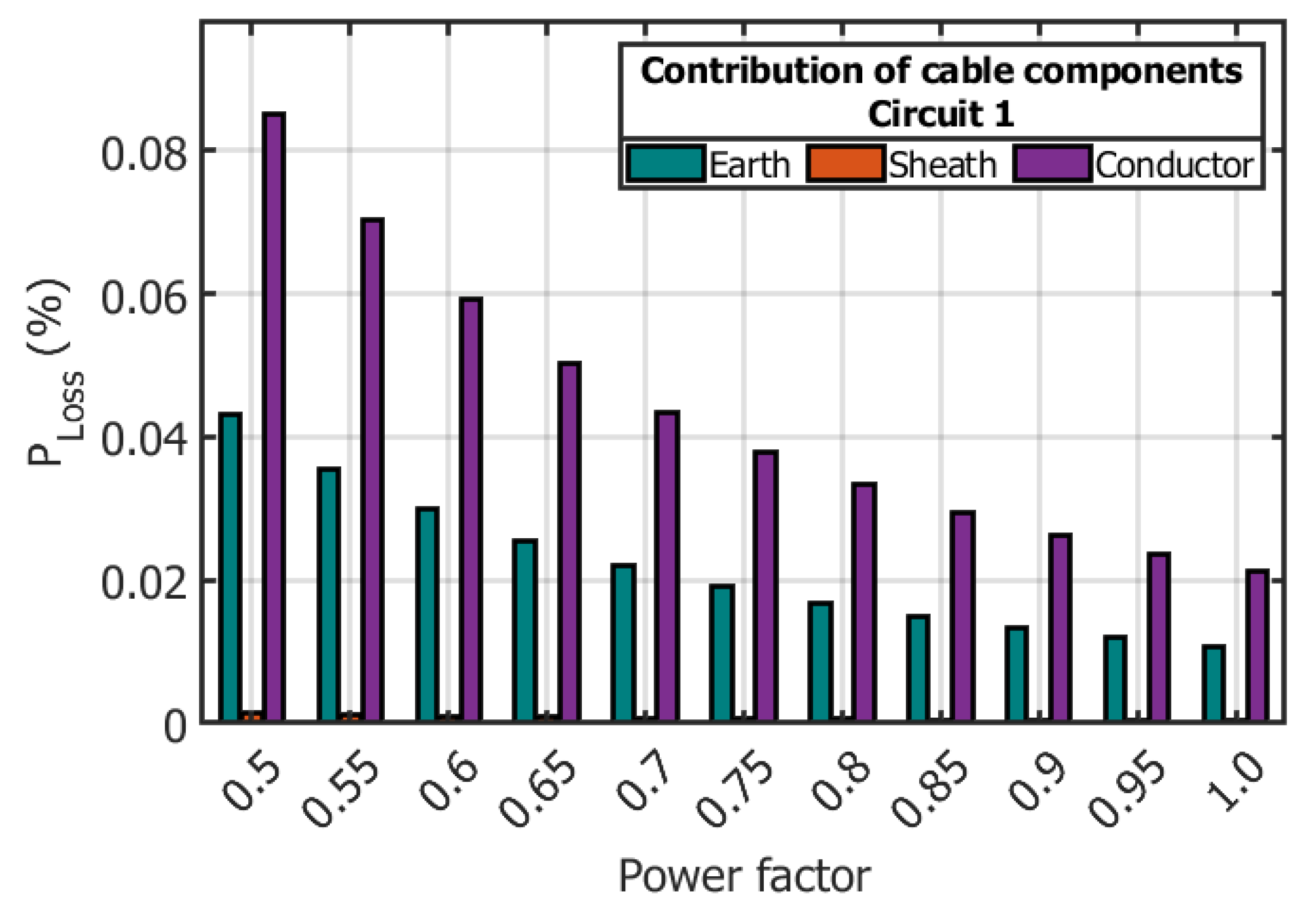
The results also show that all three contributions decrease as the power factor approaches unity. This behavior is consistent with the reduction in current magnitude associated with a lower reactive-power component. The relative predominance of the core conductor is maintained throughout the evaluated power-factor range.
6.2. Breakdown of Voltage-Drop Contributions
Figure 15 illustrates the contributions of the different cable components to the total voltage drop (ΔV) in Circuit 1 as a function of power factor over the range from 0.5 to 1.0. The analysis considers the earth-return path, metallic sheath, core conductor, and insulation within the complete electromagnetic cable model.
The component contributions are evaluated by successively modifying the corresponding component properties in the electromagnetic model and calculating the resulting voltage-drop response. The earth-return contribution is evaluated by reducing the soil resistivity to a negligible value in the model. The metallic-sheath contribution is estimated by assigning a negligible sheath resistivity in the model. The remaining contribution is associated with the insulation.
As shown in Figure 15, the earth-return path provides the largest contribution to the voltage drop over the investigated power-factor range. At low power factors, its contribution is approximately 0.088%, decreasing progressively to approximately 0.044% at unity power factor. The insulation contribution is the second largest, decreasing from approximately 0.050% at pf = 0.5 to approximately 0.025% at pf = 1.0. The metallic sheath and core conductor exhibit smaller contributions throughout the evaluated range.
At the reference operating condition of pf = 0.9, the earth-return path remains the dominant component, followed by the insulation, metallic sheath, and core conductor. These results indicate that the earth-return path has a significant influence on the voltage regulation predicted by the complete electromagnetic cable model. Consequently, neglecting earth-return effects may lead to an incomplete representation of voltage-drop behavior in medium-voltage underground collection systems.
The component-level results should be interpreted as a model-based sensitivity analysis of the voltage-drop response rather than as strictly independent physical voltage drops, since modifying one component of the electromagnetic model can also affect the resulting coupled system response.
6.3. Discussion
The results demonstrate that the choice of cable representation affects both the magnitude and the physical interpretation of the medium-voltage collection-system response. The comparison between the complete frequency-dependent ZY model and the simplified RDC,core representation shows that the latter can underestimate both active-power losses and voltage-drop magnitude under the evaluated operating conditions.
Figure 15.
Contributions of the earth-return path, metallic sheath, core conductor, and insulation to the total voltage drop (ΔV) as a function of power factor for Circuit 1.
Figure 15.
Contributions of the earth-return path, metallic sheath, core conductor, and insulation to the total voltage drop (ΔV) as a function of power factor for Circuit 1.
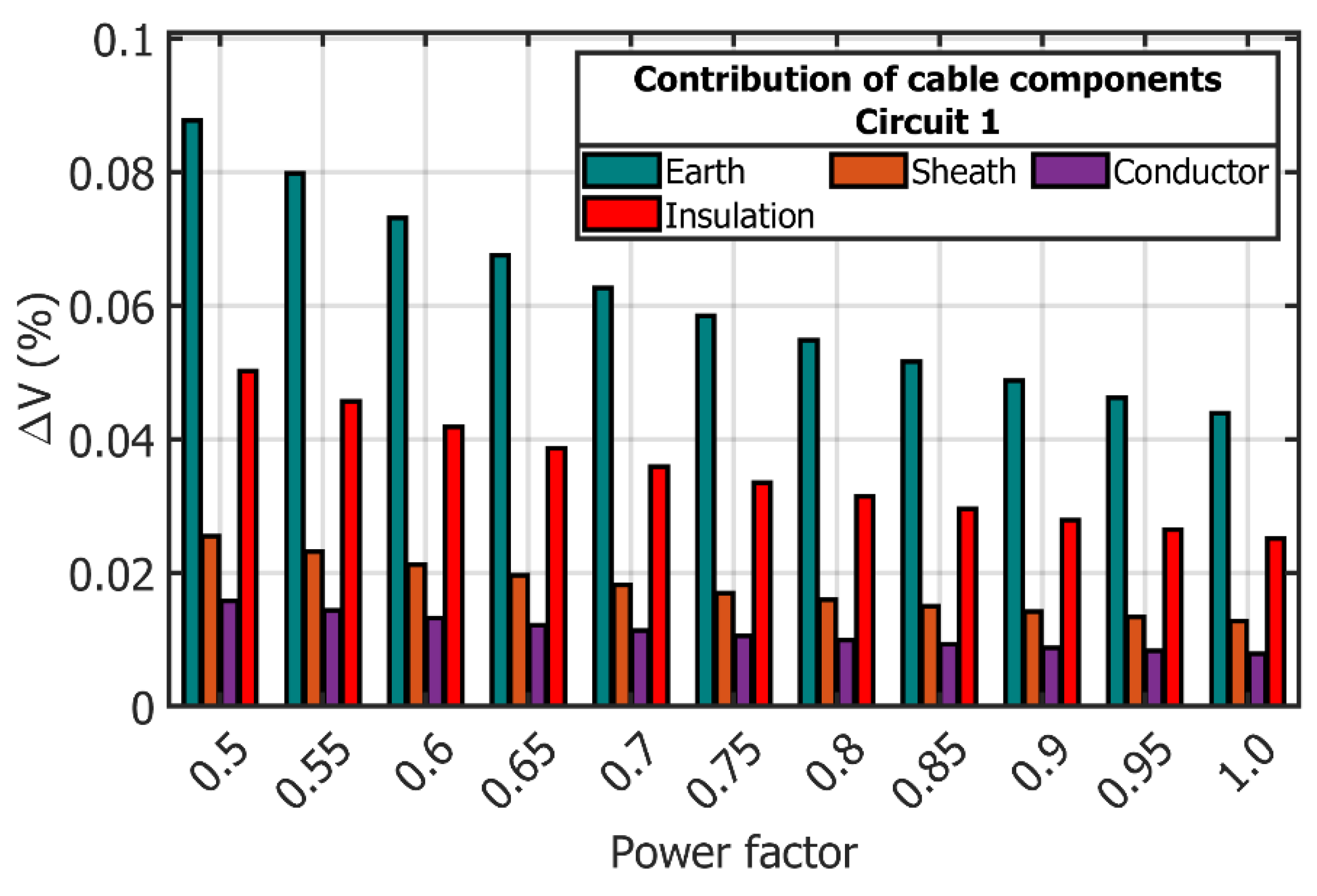
The component-level analysis provides additional insight into these differences. The core conductor is the dominant contributor to active-power dissipation, whereas the earth-return path has a significant influence on voltage-drop behavior. These findings indicate that conductor losses and voltage regulation are governed by different aspects of the coupled cable system. These findings indicate that conductor losses and voltage regulation are governed by different aspects of the coupled cable system. Consequently, reducing conductor losses alone does not necessarily eliminate the voltage-regulation effects associated with the earth-return path and electromagnetic coupling.
The comparison of earth-return formulations further indicates that the most accurate formulations are not necessarily the most computationally demanding alternatives. The Saad–Gaba–Giroux and Wedepohl-series formulations provide the closest agreement with the RSCAD benchmark over the evaluated frequency range, supporting their use when frequency-dependent cable modeling is required for planning, performance assessment, or detailed electromagnetic validation.
The maximum relative underestimation of active-power losses of approximately 60% obtained with the constant core-resistance representation should be interpreted as an operating-point difference rather than as a direct estimate of annual energy losses. This value quantifies the discrepancy between the two electrical representations under the evaluated operating conditions and should not be interpreted as a 60% reduction in annual project revenue or energy production.
From a practical perspective, the required cable-model fidelity depends on the specific design objective. A constant DC resistance may be adequate for preliminary assessments in which approximate conductor losses are sufficient. However, voltage-regulation studies, cable optimization, detailed performance assessment, and validation against electromagnetic simulation tools benefit from frequency-dependent parameters and explicit treatment of the earth-return path.
7. Techno-Economic Implications
The technical loss results are interpreted in the context of the project-level economic model developed for the same 7.5 MW wind-farm case study. The assessment considers a five-turbine wind farm, the selected underground-cable configurations, annual energy production, electricity-market revenues, operation and maintenance costs, a 20-year project lifetime, a real discount rate of 4%, and revenues associated with Clean Energy Certificates (CEL). The supporting thesis reports a capital-cost reference of 1700 USD/kW and incorporates cable procurement costs based on the economic assumptions adopted for the study [20].
The techno-economic indicators are obtained from the project cash-flow profiles generated by the economic model. Return on investment (ROI), internal rate of return (IRR), simple payback period, and discounted payback period are evaluated from the corresponding cash-flow series for each economic scenario and electrical representation. These indicators are commonly used to assess the economic feasibility of wind-farm projects under different technical and financial assumptions [17].
The purpose of this section is to assess how the differences identified in the electromagnetic model may affect project-level economic indicators. Because the electrical losses depend on the time-varying operating conditions of the wind farm, the operating-point differences reported in Section 6 are not directly interpreted as equivalent annual energy or revenue differences.
7.1. Annual Energy Losses
The annual energy loss depends on the time-varying power dissipated by the collection network and therefore cannot be obtained by directly multiplying a single operating-point loss percentage by the annual energy production. A rigorous annual energy-loss estimate requires the electrical-loss model to be evaluated over the wind-farm production time series, including the corresponding loading level and power factor for each time interval.
For an operating profile divided into time intervals (i), the annual energy dissipated in the collection network can be calculated as:
where Ploss(ti) is the electrical power dissipated by the collection network during time interval i, Δt is the duration of each time interval, and N is the total number of time intervals in the annual operating profile.
The corresponding annual economic value of the lost electricity is
where CE(ti) is the applicable electricity value during time interval i.
In the present economic model, the annual production and operating profiles are represented using time-series data over the 8760-hour reference year. Consequently, the annual economic impact of electrical losses is determined from the corresponding time-dependent operating conditions rather than from a single-rated operating point.
Accordingly, the operating-point loss percentages reported in Section 6 are treated as model-level indicators of the electrical-loss behavior. They should not be directly multiplied by the estimated annual energy production of 28.48 GWh unless the corresponding power-factor, loading, and production-time distributions are explicitly incorporated.
7.2. Economic Effect of the DC Approximation
The economic effect of the DC approximation is evaluated by comparing the financial indicators obtained from the AC and DC electrical representations under the documented economic assumptions. The incremental annual economic impact associated with the difference in electrical losses can be expressed as:
where (ΔCloss) represents the difference in the annual economic cost associated with the electrical losses predicted by the two electrical representations.
The electromagnetic model establishes the direction and magnitude of the difference in predicted electrical losses at the evaluated operating points, whereas the corresponding annual monetary impact depends on the wind-farm production profile, loading conditions, power-factor distribution, and applicable electricity value over time. Therefore, the maximum relative underestimation of approximately 60% reported in Section 6 should not be interpreted as a 60% reduction in annual project revenue.
Instead, the economic effect of the DC approximation must be determined by integrating the difference in electrical losses over the complete annual operating profile. Under the economic assumptions adopted in this case study, the resulting differences between the AC and DC financial indicators are comparatively small at the project level, despite the larger differences observed in the operating-point electrical-loss and voltage-drop results.
7.3. Case-Study Economic Indicators
The economic evaluation compares the complete AC electromagnetic representation with the simplified DC representation for five 1.5 MW wind turbines, corresponding to a total installed capacity of 7.5 MW. The economic model incorporates annual energy production, electrical losses, capital expenditure, operation and maintenance costs, electricity-market revenues, a 20-year project lifetime, a real discount rate of 4%, and revenues associated with Clean Energy Certificates (CEL). The supporting thesis reports a capital-cost reference of 1700 USD/kW and an operation and maintenance cost equivalent to 2% of the corresponding reference cost [20].
The five turbines provide individual net annual energy production values ranging from 5.432 to 5.884 GWh, corresponding to a combined net annual energy production of approximately 28.484 GWh/year [20].
Table VII summarizes the financial indicators obtained for the AC and DC electrical representations under the economic scenarios considered in the study.
Five economic scenarios are considered to evaluate the effects of gross and net energy production, taxes, and Clean Energy Certificate (CEL) revenues. REPG represents the gross economic case; REPN represents the net economic case; REPNT represents the net case including taxes; REPC represents the net case including CEL revenues; and REPCT represents the net case including both CEL revenues and taxes. The same financial evaluation framework is applied to the AC and DC electrical representations to ensure a consistent comparison of their project-level economic performance.
The results in Table VII show that the economic indicators obtained with the AC and DC representations are generally similar, despite the substantially different electrical-loss and voltage-drop predictions identified in the electromagnetic analysis. For the gross economic results (REPG), both representations yield a ROI of 13.9866%, an IRR of 11.9605%, a payback period of 7.1497 years, and a discounted payback period of 8.5706 years. For the net-results scenario (REPN), the AC model yields a ROI of 13.2895%, an IRR of 11.8826%, a payback period of 7.5248 years, and a discounted payback period of 9.1273 years, while the corresponding DC values are 13.2520%, 11.8378%, 7.5460 years, and 9.1575 years, respectively.
When taxes are included (REPNT), the ROI decreases to 10.4353% for the AC representation and 10.4110% for the DC representation. The scenarios incorporating CEL revenues provide the strongest financial performance. For REPC, the AC representation yields a ROI of 15.9027%, an IRR of 14.9168%, a payback period of 6.2883 years, and a discounted payback period of 7.3767 years. The corresponding DC values are 15.8587%, 14.8670%, 6.3057 years, and 7.3996 years, respectively.
Because income tax is applied only after the break-even point, the resulting REPCT indicators remain close to those obtained with REPC, while reflecting the tax burden in the post-break-even cash flows. Thus, the inclusion of CEL revenues improves the reported project profitability and reduces the investment recovery period. Nevertheless, the difference between the detailed AC and simplified DC representations remains relatively small at the project-level financial scale for the documented case study.
These results indicate that the frequency-dependent model provides a materially more detailed characterization of cable losses and voltage regulation, while its direct effect on the project-level financial indicators remains limited under the economic assumptions adopted in this case study [20].
The economic results should be interpreted together with the operating-point electrical results presented in Section 6. The differences in the electromagnetic predictions do not translate directly into equivalent differences in annual project revenues because the economic model depends on the complete annual production and operating profile.
For the gross economic results (REPG), both the AC and DC models yield a ROI of 13.9866%, an IRR of 11.9605%, a payback period of 7.1497 years, and a discounted payback period of 8.5706 years.
7.4. Life-Cycle Comparison of Cable Alternatives
For cable alternative (j), the life-cycle cost can be expressed as
where C(0,j) is the initial cable and installation cost, C(loss,j,t) is the annual economic cost associated with electrical losses, C(OM,j,t) is the operation and maintenance cost, and (r) is the real discount rate.
The electromagnetic model provides the electrical-loss component of this formulation, whereas procurement, installation, maintenance, electricity-value, and discount-rate inputs must be documented independently for each cable alternative. Consequently, the life-cycle comparison presented here should be interpreted as a framework for integrating the frequency-dependent electrical results into the economic assessment rather than as a complete life-cycle-cost calculation unless all corresponding economic inputs are explicitly available.
The proposed framework allows different cable alternatives to be compared by combining their initial investment costs with the present value of electrical losses and operation and maintenance costs over the project lifetime. This approach provides a direct connection between the frequency-dependent electrical model and cable-selection decisions based on both technical performance and economic criteria.
7.5. Sensitivity Analysis and Decision Criteria
The economically relevant sensitivity parameters include the electricity value, annual operating hours or capacity factors, cable and installation costs, discount rate, project lifetime, treatment of CEL revenues, and AC cable resistance.
The sensitivity analysis is used to evaluate the robustness of the project-level economic indicators under variations in the parameters that directly affect investment, operating costs, and electrical losses. Particular attention is given to the AC cable resistance because variations in resistance directly affect the resistive losses predicted by the electromagnetic model.
A cable alternative can be considered economically preferable when the present value of the additional investment is lower than the present value of the avoided electrical loss and maintenance costs over the project lifetime. In general, the decision criterion can be expressed as a comparison between the incremental investment cost and the present value of the corresponding economic benefits.
For the present case study, the similarity of the AC and DC financial indicators indicates that the choice between the detailed and simplified electrical representations has a limited influence on project-level profitability under the documented economic assumptions. However, this result does not imply that the two representations provide equivalent electrical predictions. As demonstrated in Section 6, significant differences remain in the predicted active-power losses and voltage drop at specific operating conditions.
Therefore, the selection of the electrical model should consider both the purpose of the analysis and the required level of accuracy. The detailed frequency-dependent model is preferable when cable losses, voltage regulation, electromagnetic coupling, and earth-return effects must be characterized, whereas the simplified DC representation may be sufficient for preliminary economic assessments when only approximate project-level financial indicators are required.
7.5.1. AC Cable Resistance Sensitivity
A dedicated sensitivity analysis was performed by multiplying the complete AC cable resistance matrix by factors ranging from 1 to 6, corresponding to resistance increases from 0% to 500%. The base case was first evaluated using the economic model. At a 0% resistance increase, the reported REPC results yield a ROI of 15.8587%, an IRR of 14.8670%, a payback period of 6.3057 years, and a discounted payback period of 7.3996 years.
The 0–500% resistance-increase range was selected as a parametric sensitivity analysis to quantify the robustness of the project-level financial indicators under progressively larger resistance deviations. This range is not intended to represent a typical physical uncertainty range for the cable conductor.
Increasing the AC cable resistance results in a monotonic deterioration of all four financial indicators. At a 500% resistance increase, corresponding to a six-fold resistance factor, the ROI decreases to 15.3008% and the IRR to 14.2319%, while the payback period increases to 6.5356 years and the discounted payback period increases to 7.7021 years.
Table VIII summarizes the resulting sensitivity of the REPC financial indicators to the AC cable resistance. The corresponding trends in ROI and IRR are illustrated in Figure 16. The resulting payback and discounted payback trends are shown in Figure 17.
The sensitivity results show a nearly linear deterioration of the financial indicators over the evaluated resistance range. From 0% to 500% resistance increase, the ROI decreases by 0.5579 percentage points and the IRR decreases by 0.6351 percentage points, while the payback period and discounted payback period increases by 0.2299 and 0.3025 years, respectively.
This behavior is consistent with the electrical-loss mechanism identified in Section 6: increasing cable resistance increases resistive losses and consequently reduces the net economic performance of the project. Importantly, the reproduction of the base-case financial indicators provides a consistency check between the sensitivity analysis and the corresponding economic model.
7.6. Economic Interpretation and Limitations
The principal economic implication is that the frequency-dependent cable model provides a more detailed characterization of collection-system losses and voltage regulation, while the project-level financial indicators remain comparatively close to those obtained with the simplified DC representation for the documented 7.5 MW case study.
These results support the use of the detailed electromagnetic model for technical design, cable assessment, and electrical-loss characterization without implying that the operating-point differences translate directly into an equivalent percentage change in annual project revenue. The economic impact of the frequency-dependent model depends on the temporal distribution of wind-farm loading, power factor, electricity value, and other operating conditions throughout the year.
The approximately 60% maximum relative difference in active-power loss identified in Section 6 should therefore be interpreted as an operating-point electrical-model discrepancy rather than as an equivalent annual economic loss. A rigorous economic assessment requires the frequency-dependent electrical model to be evaluated over the complete annual production profile.
A broader techno-economic assessment should consider alternative cable cross-sections, installation configurations, production time series, electricity-price scenarios, capacity factors, and discount-rate assumptions while using the same frequency-dependent loss model. Such an approach would allow the electrical effects identified in this study to be translated into annual energy losses and life-cycle economic indicators with greater quantitative confidence.
The present case study is therefore primarily intended to demonstrate the technical significance of frequency-dependent cable modeling and its potential integration into techno-economic assessment. The limited difference between the AC and DC project-level financial indicators should be interpreted within the specific assumptions and operating conditions documented for the 7.5 MW wind farm.
8. Conclusions
This study developed and validated a frequency-dependent electromagnetic ZY model for medium-voltage underground collection networks and applied it to a 7.5 MW wind-farm case study in the Isthmus of Tehuantepec, Oaxaca, Mexico. The main findings are summarized as follows:
Model validation: The MATLAB-based framework shows close agreement with the RSCAD benchmark over the frequency range from 10 Hz to 1 MHz. Among the evaluated earth-return approximations, the Saad–Gaba–Giroux and Wedepohl-series formulations provide the closest agreement with the reference results.
Power-loss bias: At pf=0.9, the constant DC core-resistance representation underestimates the modeled active-power losses, with a maximum relative underestimation of approximately 60% across the evaluated operating conditions and circuits. This result indicates that frequency-dependent cable effects should be considered when detailed electrical loss estimates are required.
Voltage-regulation bias: At pf=0.9, the complete ZY model predicts voltage drops of approximately 0.68% and 1.55% for Circuits 1 and 2, respectively, whereas the simplified DC representation predicts values below 0.15% for both circuits. The difference is therefore relevant to voltage-regulation assessment in medium-voltage underground collection systems.
Component-level losses: The core conductor is the dominant contributor to active-power dissipation in the evaluated Circuit 1 conditions, followed by the earth-return path and metallic sheath. This result indicates that conductor losses remain the principal source of active-power dissipation in the analyzed cable configuration.
Earth-return influence: The component-level equivalent-resistance analysis indicates that the earth-return path has a significant influence on the equivalent phase resistance and voltage-drop behavior. Consequently, explicit representation of the earth-return path is relevant when detailed voltage-regulation characteristics are required.
Techno-economic implication: For the documented 7.5 MW case study, the CEL-inclusive scenario provides the strongest reported financial performance. The AC and DC representations produce comparatively similar project-level financial indicators under the adopted economic assumptions, despite the larger differences observed in the operating-point electrical results.
Resistance sensitivity: The AC cable-resistance sensitivity analysis shows a monotonic deterioration of the reported financial indicators as resistance increases from 0% to 500%. For the evaluated sensitivity range, the REPC ROI decreases from 15.8587% to 15.3008%, while the IRR decreases from 14.8670% to 14.2319%. The payback period increases from 6.3057 to 6.5356 years, and the discounted payback period increases from 7.3996 to 7.7021 years.
Overall, the results demonstrate that frequency-dependent cable modeling provides a more comprehensive representation of the electrical behavior of medium-voltage underground collection systems, particularly when active-power losses, voltage regulation, electromagnetic coupling, and earth-return effects are considered simultaneously. At the same time, the case study shows that differences in electrical-model fidelity do not necessarily translate into proportional differences in project-level financial indicators. Therefore, the appropriate cable representation should be selected according to the objectives of the analysis and the required level of electrical and economic accuracy.
Acknowledgments
The authors are grateful for the support provided by the Secretariat of Science, Humanities, Technology and Innovation (SECIHTI) and the Graduate Studies Division of the University of the Isthmus (UNISTMO).
Author Contributions
A.K.L.G.: Conceptualization, methodology, investigation, software, writing—original draft preparation, writing—review and editing, and project administration; R.I.C.: investigation, supervision, and writing—original draft preparation; G.M.R.: review and editing; E.D.R.: review and editing. All authors have read and agreed to the published version of the manuscript.
Funding
This research received no external funding.
Institutional Review Board Statement
Not applicable.
Informed Consent Statement
Not applicable.
Data Availability Statement
The data supporting the findings of this study are available from the corresponding author upon reasonable request.
Conflicts of Interest
The authors declare no conflicts of interest.
Abbreviations
The following abbreviations are used in this manuscript:
| AC | Alternating Current |
| DC | Direct Current |
| MV | Medium Voltage |
| ZY | Frequency-Dependent Series Impedance and Shunt Admittance Model |
| RSCAD | Real-Time Simulation Computer-Aided Design |
| IEC | International Electrotechnical Commission |
| WMO | World Meteorological Organization |
| CERTE | Regional Center for Wind Technology |
| XLPE | Cross-Linked Polyethylene |
| EPR | Ethylene Propylene Rubber |
| PVC | Polyvinyl Chloride |
| RMSE | Root Mean Square Error |
| WS | Wedepohl Series |
| GAEP | Gross Annual Energy Production |
| NAEP | Net Annual Energy Production |
| CEL | Clean Energy Certificates |
| ROI | Return on Investment |
| IRR | Internal Rate of Return |
| LCC | Life-Cycle Cost |
| REPG | Gross Economic Results |
| REPN | Net Economic Results |
| REPNT | Net Economic Results Including Taxes |
| REPC | Net Economic Results Including Clean Energy Certificate Revenues |
| REPCT | Net Economic Results Including Clean Energy Certificate Revenues and Taxes |
References
- Elliott, D.; Schwartz, M.; Scott, G.; Heimiller, D.; George, R. Wind Energy Resource Team, “Wind Energy Resource Atlas of Oaxaca,” National Renewable Energy Laboratory (NREL), Golden, CO, USA, Tech. Rep. NREL/TP-500-34519. 2003. [CrossRef]
- International Electrotechnical Commission (IEC). IEC Standard 61400-1:2019; Wind energy generation systems – Part 1: Design requirements. Feb 2019.
- Papadopoulos, T. A.; Pippi, K. D.; Pompodakis, E. E.; Kryonidis, G. C.; Chrysochos, A. I. Evaluation of electric power losses in wind farms considering temperature-dependent power flow. Sustain. Energy Grids Netw. 2025, vol. 44, art.(no. 102003). [Google Scholar] [CrossRef]
- Dommel, H. W. Electromagnetic Transients Program Reference Manual (EMTP Theory Book), prepared for Bonneville Power Administration; Portland, OR, USA, 1986. [Google Scholar]
- Velasco, J. Finite-Element Modeling of Thin Wires Including Skin and Proximity Effects. Ph.D. dissertation, Dept. Elect. Eng., Univ. Liège, Liège, Belgium, 2022. [Google Scholar]
- Jabłoński, P.; Zaręba, M.; Szczegielniak, T.; Gołębiowski, J. Influence of the Skin and Proximity Effects on the Thermal Field in Flat and Trefoil Three-Phase Systems with Round Conductors. Energies 2024, vol. 17(no. 7), 1713. [Google Scholar] [CrossRef]
- Pollaczek, F. Über das Feld eines unendlich langen wechselstromdurchflossenen Leiters im Erdboden. Elektr. Nachrichtentechnik 1926, vol. 3, 339–359. [Google Scholar]
- Wedepohl, L. M.; Wilcox, D. J. Transient analysis of underground power-transmission systems: system-parameter calculations. Proc. Inst. Electr. Eng. 1973, vol. 120(no. 2), 253–260. [Google Scholar] [CrossRef]
- Saad; Gaba, G.; Giroux, M. A closed-form approximation for ground return impedance of underground cables. IEEE Trans. Power Deliv. 1996, vol. 11(no. 3), 1536–1545. [Google Scholar] [CrossRef]
- Tylavsky, D. J.; Brown, K. A.; Ma, T. T. Closed-form solution for underground impedance calculations. Proc. IEEE 1986, vol. 74(no. 9), 1290–1292. [Google Scholar] [CrossRef]
- Iracheta-Cortez, R.; Flores-Guzman, N. Developing automated Hardware-In-the-Loop tests with RTDS for verifying the protective relay performance. Proc. IEEE 36th Central American and Panama Convention (CONCAPAN XXXVI), San Jose, Costa Rica, Nov. 2016; pp. 1–9. [Google Scholar] [CrossRef]
- Iracheta, R.; Flores-Guzman, N. A Taylor-Series expansion method for the accurate calculation of earth return impedance in buried cables. Proc. 2014 IEEE Central America and Panama Convention (CONCAPAN XXXIV), Panama, Panama, 2014; pp. 1–7. [Google Scholar] [CrossRef]
- Iracheta-Cortez, R. A recursive-formula for the evaluation of the earth-return impedance on buried cables. Ing. E Investig. 2015, vol. 35(no. 3), 34–43. [Google Scholar] [CrossRef]
- World Meteorological Organization (WMO). Measurement of surface wind. In Guide to Instruments and Methods of Observation (WMO-No. 8), vol. I: Measurement of Meteorological Variables, Available: wmo.int, 2021 ed.; WMO: Geneva, Switzerland, 2021; p. ch. 5. [Google Scholar]
- International Electrotechnical Commission (IEC). IEC Standard 61400-12-1:2022; Wind energy generation systems—Part 12-1: Power performance measurements of electricity producing wind turbines. 2022.
- Ortiz-Jiménez, G.; Iracheta-Cortez, R.; Martínez-Reyes, G.; Dorrego-Portela, J. R. Implementation of Bimodal Probability Density Function to Estimate the Wind Energy Potential in the Region of the Isthmus of Tehuantepec. Proc. 2023 IEEE 41st Central America and Panama Convention (CONCAPAN XLI), Tegucigalpa, Honduras, 2023; pp. 1–6. [Google Scholar] [CrossRef]
- Ángeles-Pérez, K.; Martínez-Reyes, G.; Iracheta-Cortez, R.; Otamendi-Cruz, L. A.; de la Cruz-Soto, J.; Dueñas-Reyes, E. Comparison of wind resource among physical and virtual weather stations for analyzing the economic feasibility of wind farms. Proc. 2022 IEEE 40th Central America and Panama Convention (CONCAPAN), Panama, Panama, 2022; pp. 1–6. [Google Scholar] [CrossRef]
- Ángeles-Pérez, K.; Iracheta-Cortez, R. Assessment of the Economic Viability of Low Power Wind Farms in Mexico. IEEE Lat. Am. Trans. 2024, vol. 22(no. 4), 329–338. [Google Scholar] [CrossRef]
- Iracheta-Cortez, R.; Dorrego, J. R. Analysis of the Wake Effect in the Distribution of Wind Turbines. IEEE Lat. Am. Trans. 2020, vol. 18(no. 4), 668–676. [Google Scholar] [CrossRef]
- López-González, K. Analysis of Electrical Losses in Underground Cables of Wind Farms. Master’s thesis, Master of Science in Wind Energy, Universidad del Istmo, Santo Domingo Tehuantepec, Oaxaca, Mexico, Jun 2026. [Google Scholar]
- Uribe, F. A.; Ramos-Leaños, O.; Zuniga, P. An investigation of earth and sea-return impedances of power electrical cables. Electr. Power Syst. Res. 2023, vol. 222, 109608. [Google Scholar] [CrossRef]
- De Conti, A. C. S.; Lima. Accuracy assessment of analytical expressions for the ground return impedance of underground cables. Electr. Power Syst. Res. 2026, vol. 250, 112146. [Google Scholar] [CrossRef]
Figure 1.
Underground cable transmission system. Horizontal layout with three underground cables. b) Geometry of a coaxial cable cross-section with 2 conductors.
Figure 1.
Underground cable transmission system. Horizontal layout with three underground cables. b) Geometry of a coaxial cable cross-section with 2 conductors.
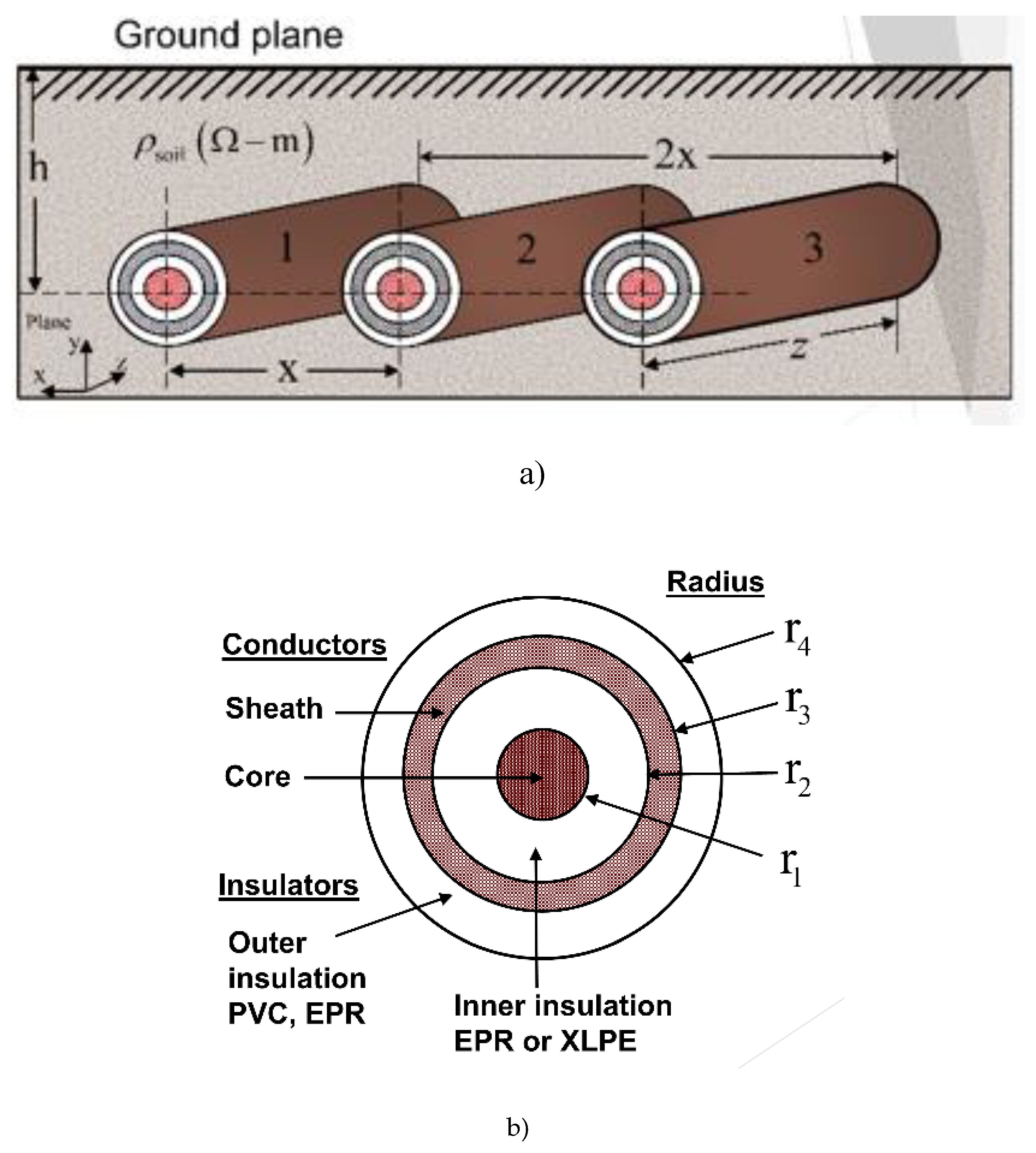
Figure 2.
Underground transmission system of 2 cables.
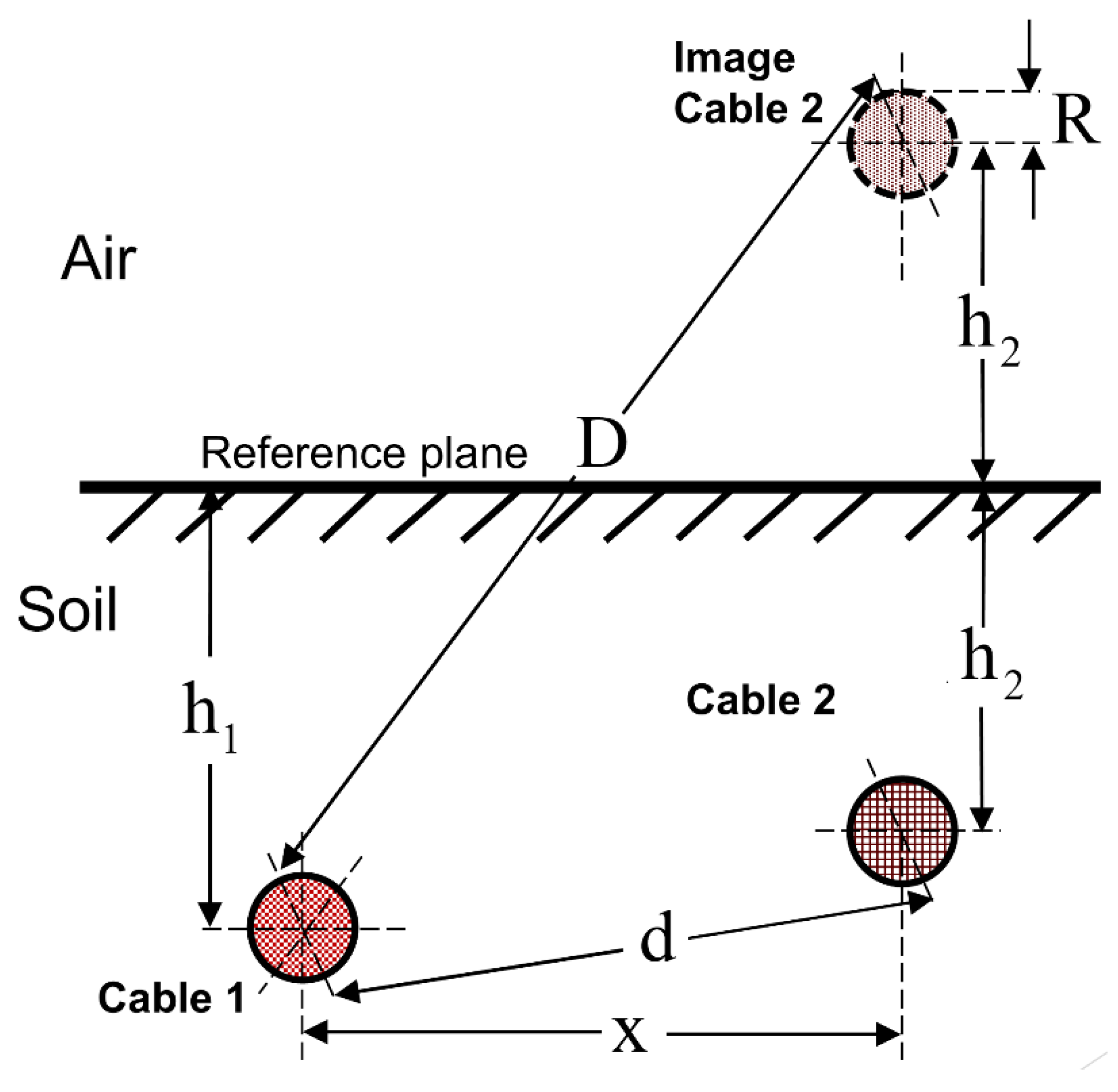
Figure 3.
Distribution of wind speeds and its fit through the Weibull function for 80 m height.
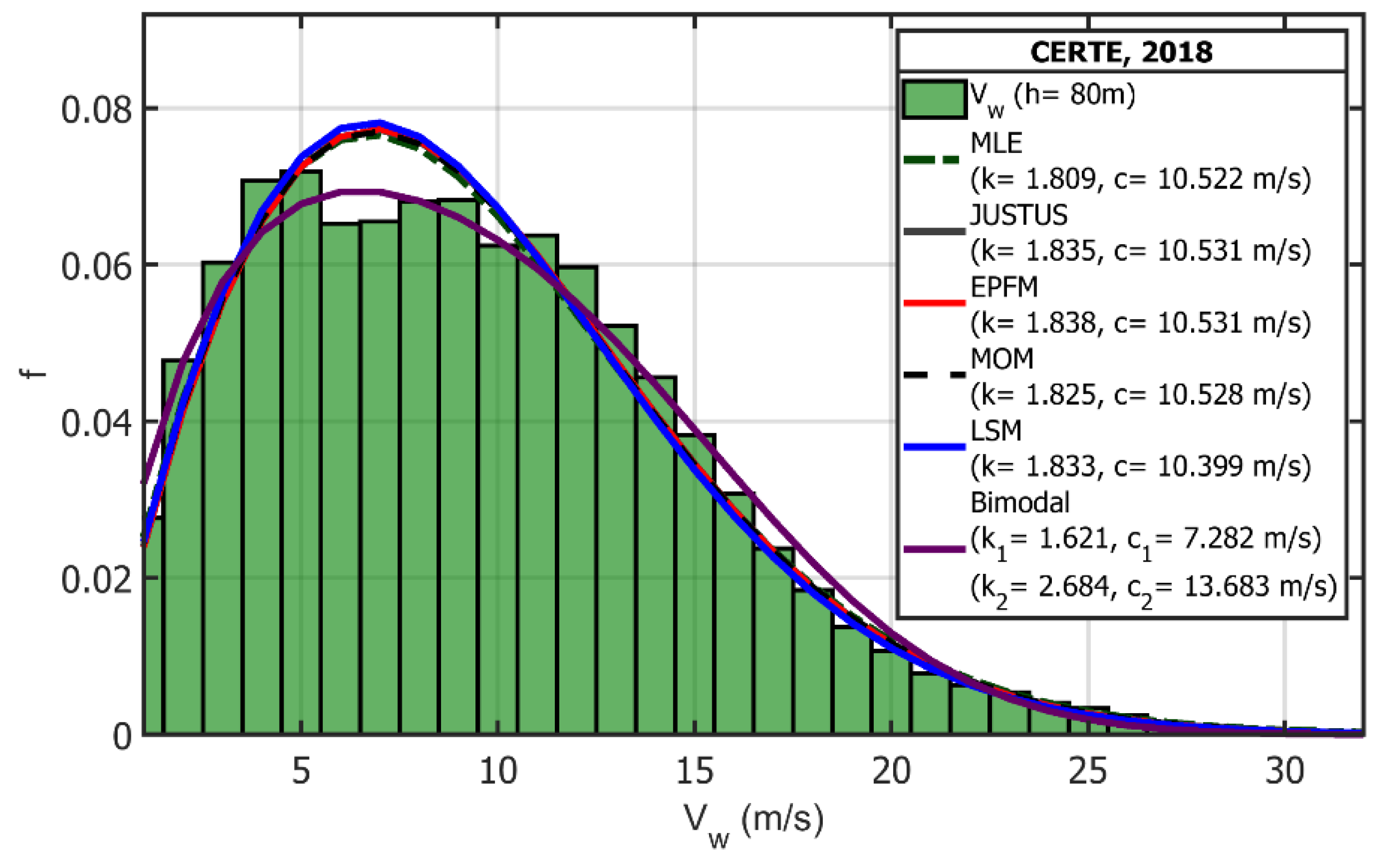
Figure 4.
Wind rose measured at 78m height.
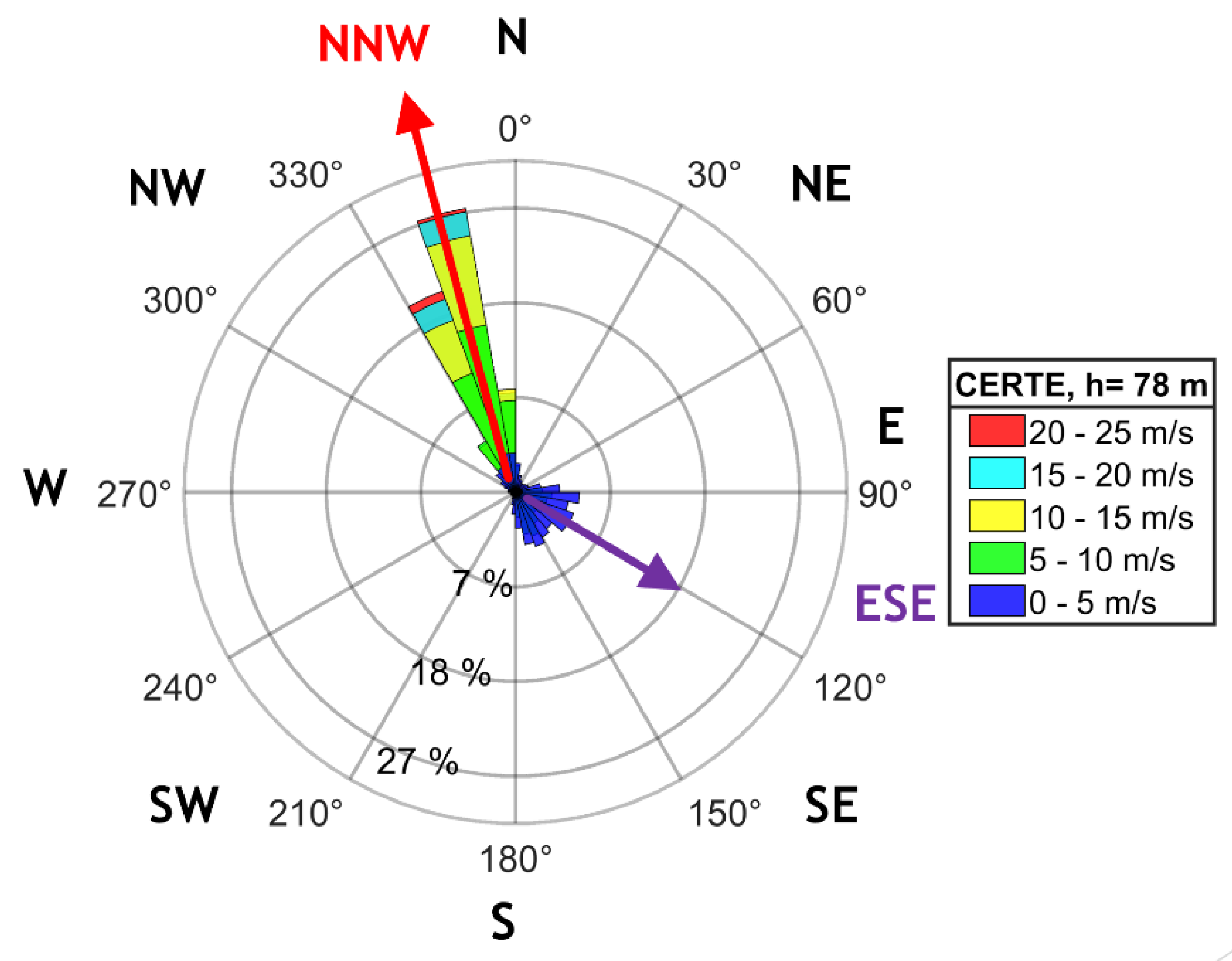
Figure 5.
Power curve of the Acciona AW-1500/70 wind turbine.
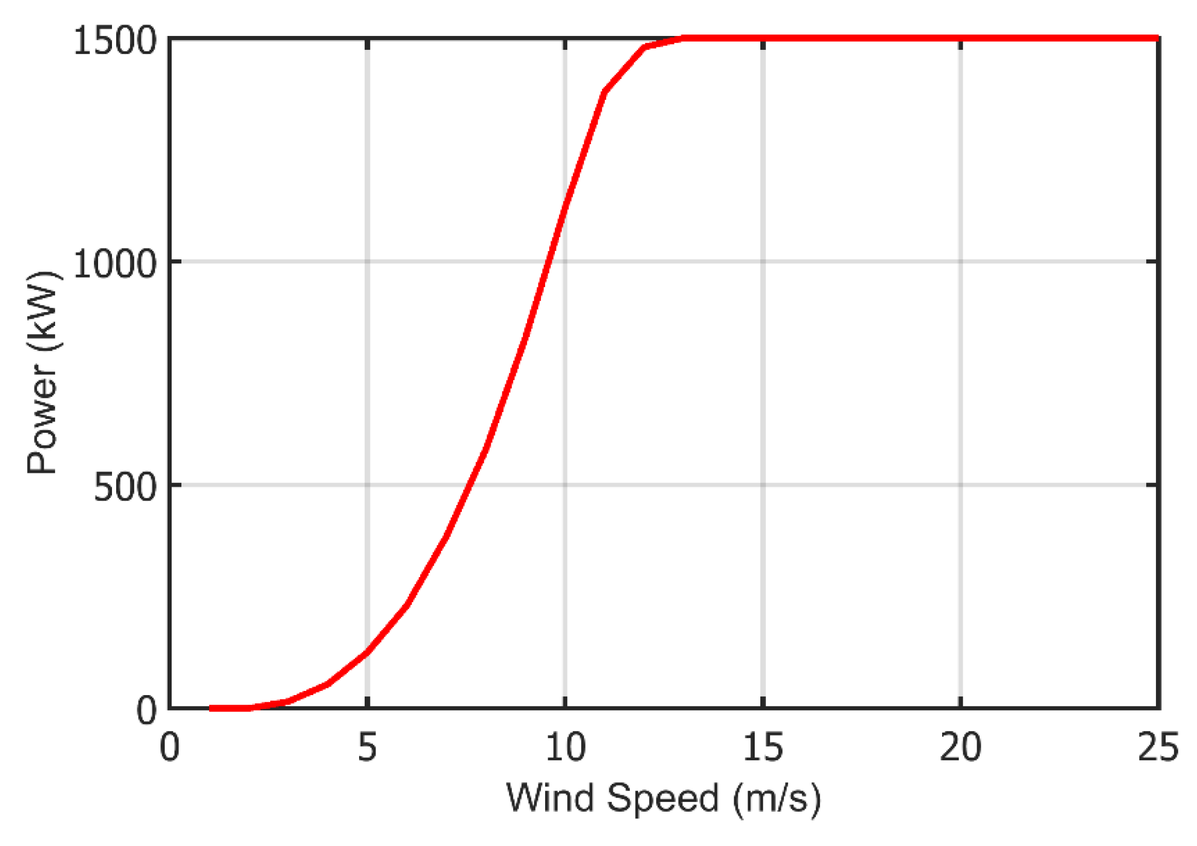
Figure 6.
Wind farm layout.
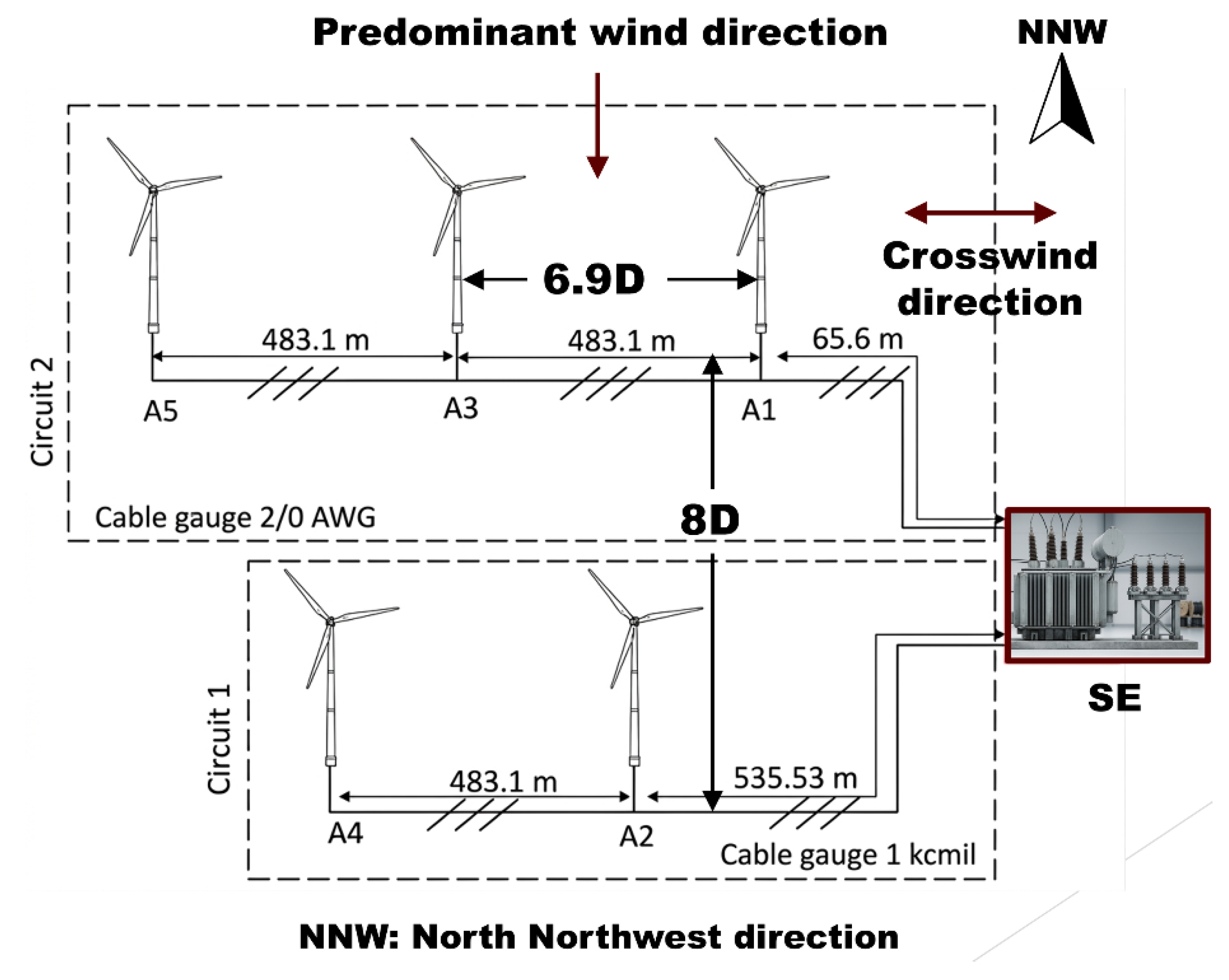
Figure 7.
Layout of the medium voltage underground cable transmission system.
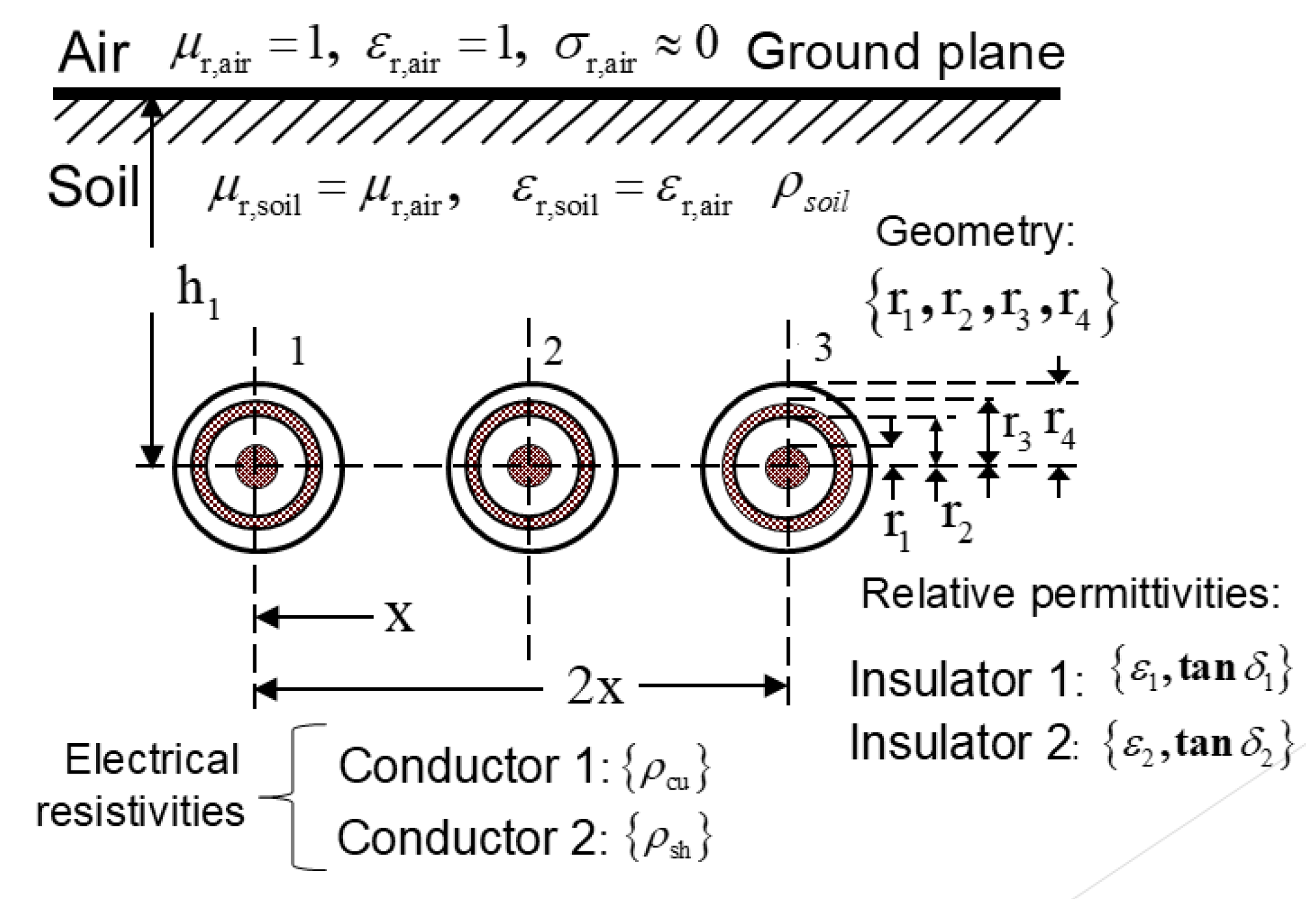
Figure 8.
Frequency response of the self-resistance (Rs,11) for cable 1 of circuit 1.
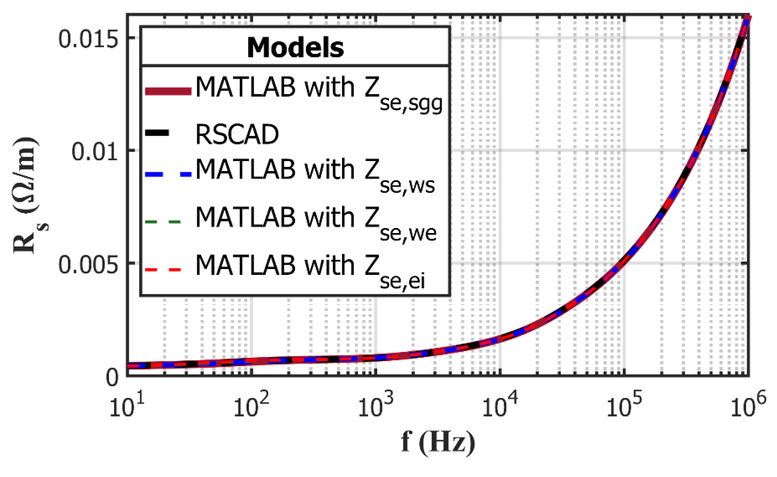
Figure 9.
Frequency response of the mutual resistance (Rm,12) between cables 1 and 2 of circuit 1.
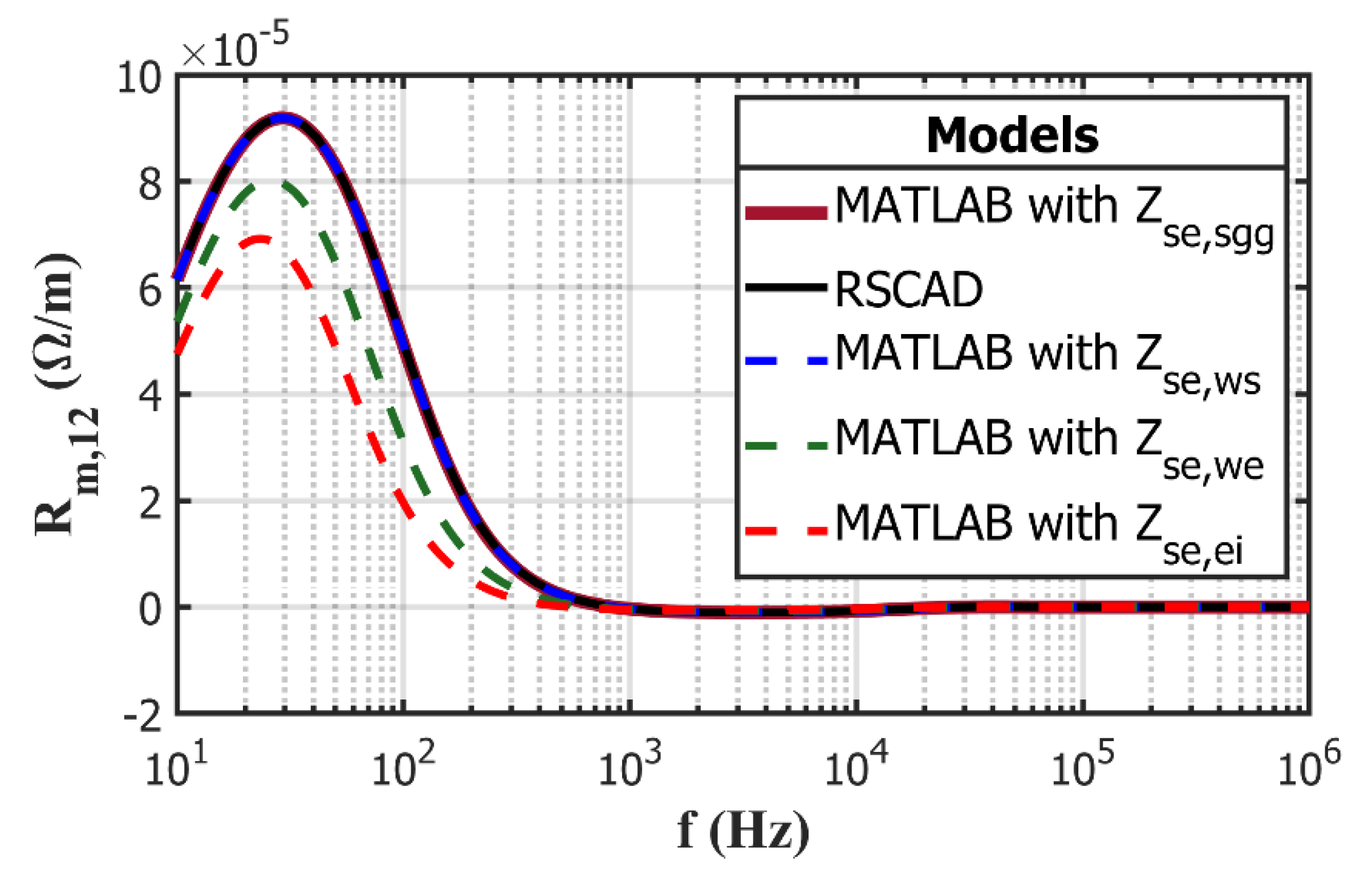
Figure 10.
Frequency response of the self-inductance waveforms (Ls,11) for the cable 1 of circuit 1.
Figure 10.
Frequency response of the self-inductance waveforms (Ls,11) for the cable 1 of circuit 1.
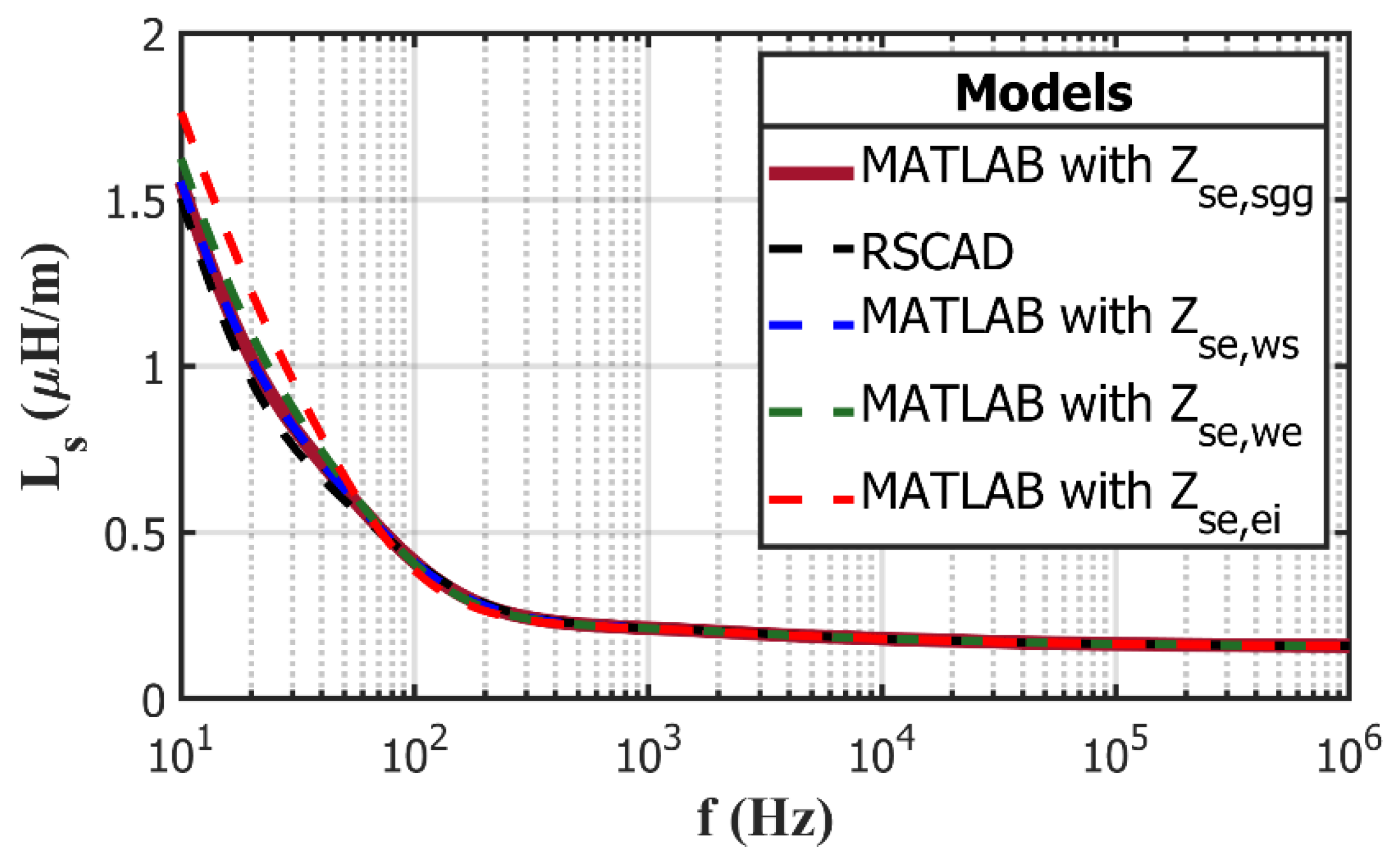
Figure 11.
Frequency response of the mutual inductance (Lm,12) among cables 1 and 2 of circuit 1.
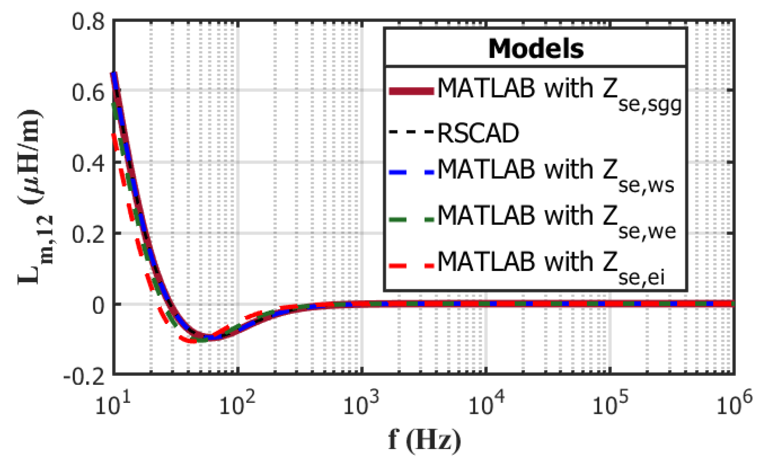
Figure 12.
Frequency response of the capacitance per unit length (C11) for Cable 1 of circuit 1.
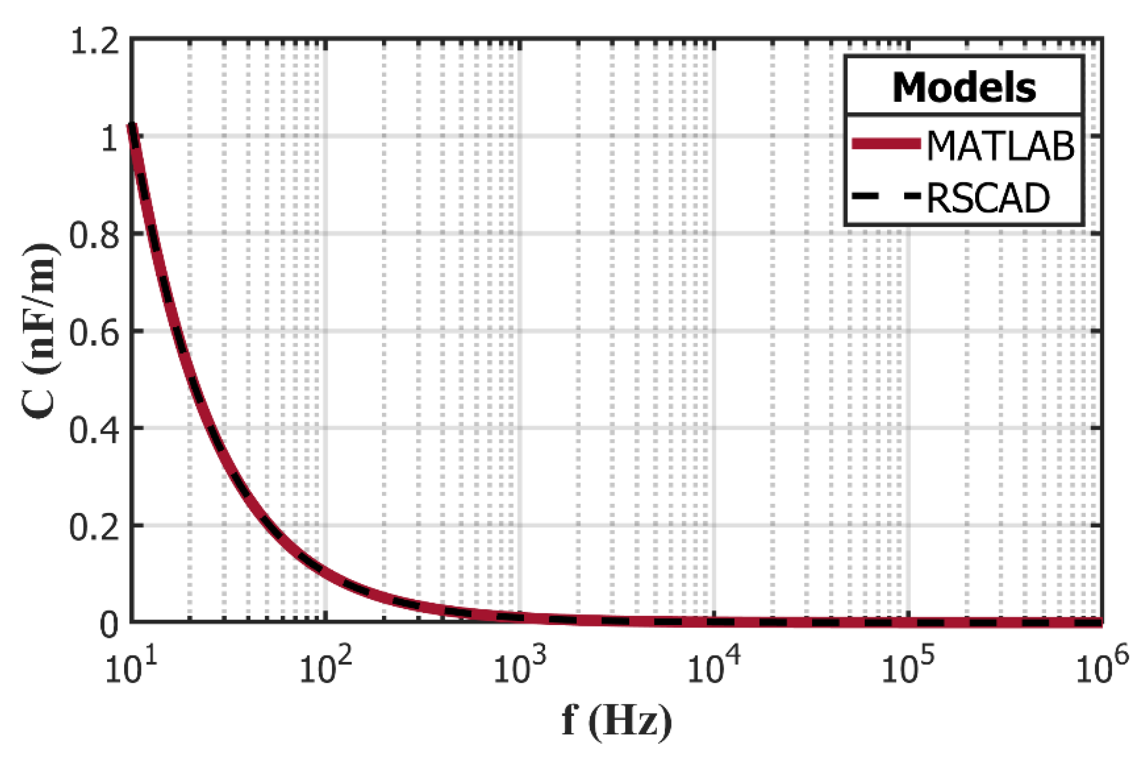
Figure 13.
Performance of the medium-voltage underground network: a) Power loss (%) vs power factor, b) Voltage drop (%) vs power factor.
Figure 13.
Performance of the medium-voltage underground network: a) Power loss (%) vs power factor, b) Voltage drop (%) vs power factor.
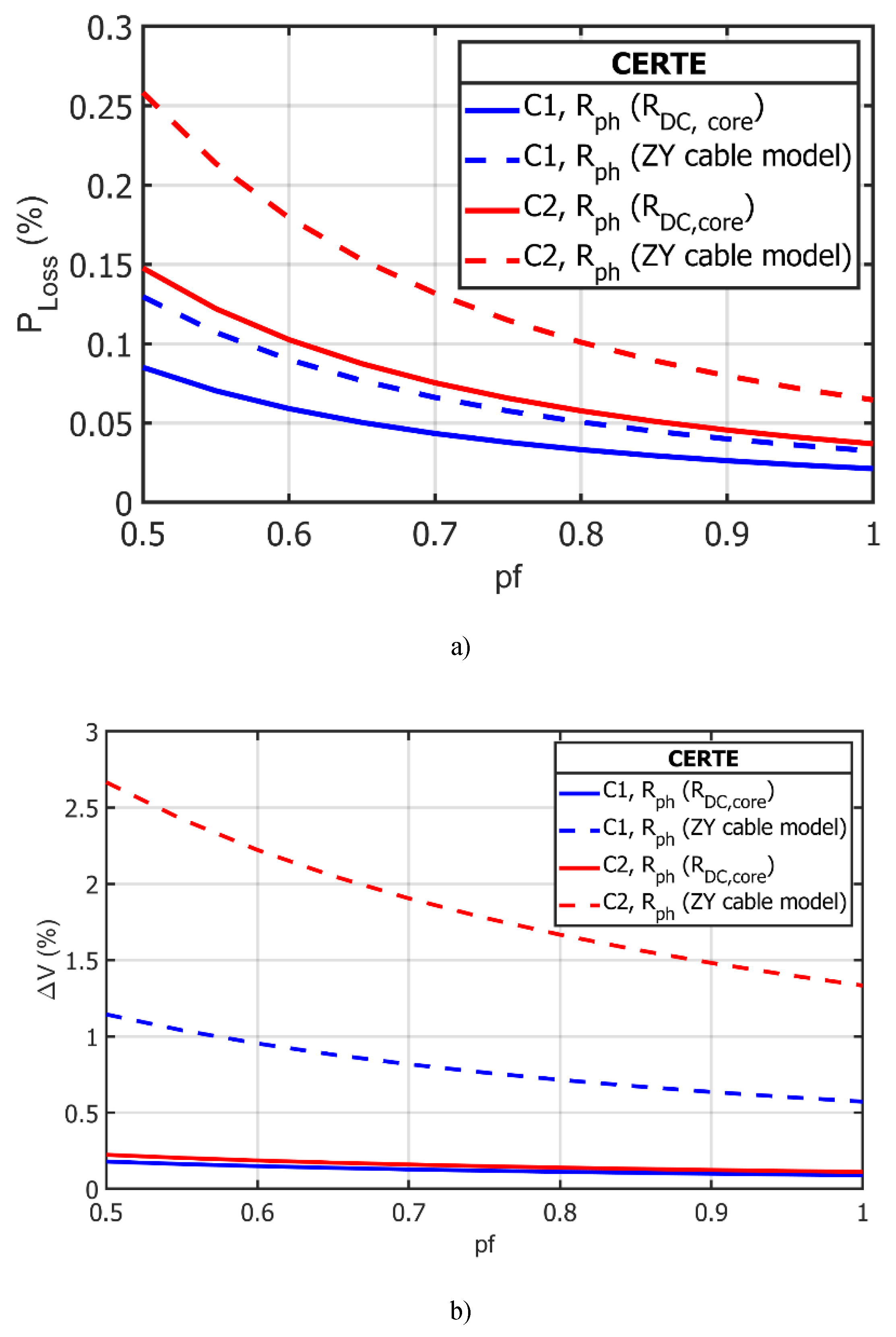
Figure 16.
REPC ROI and IRR as a function of AC cable resistance increase.
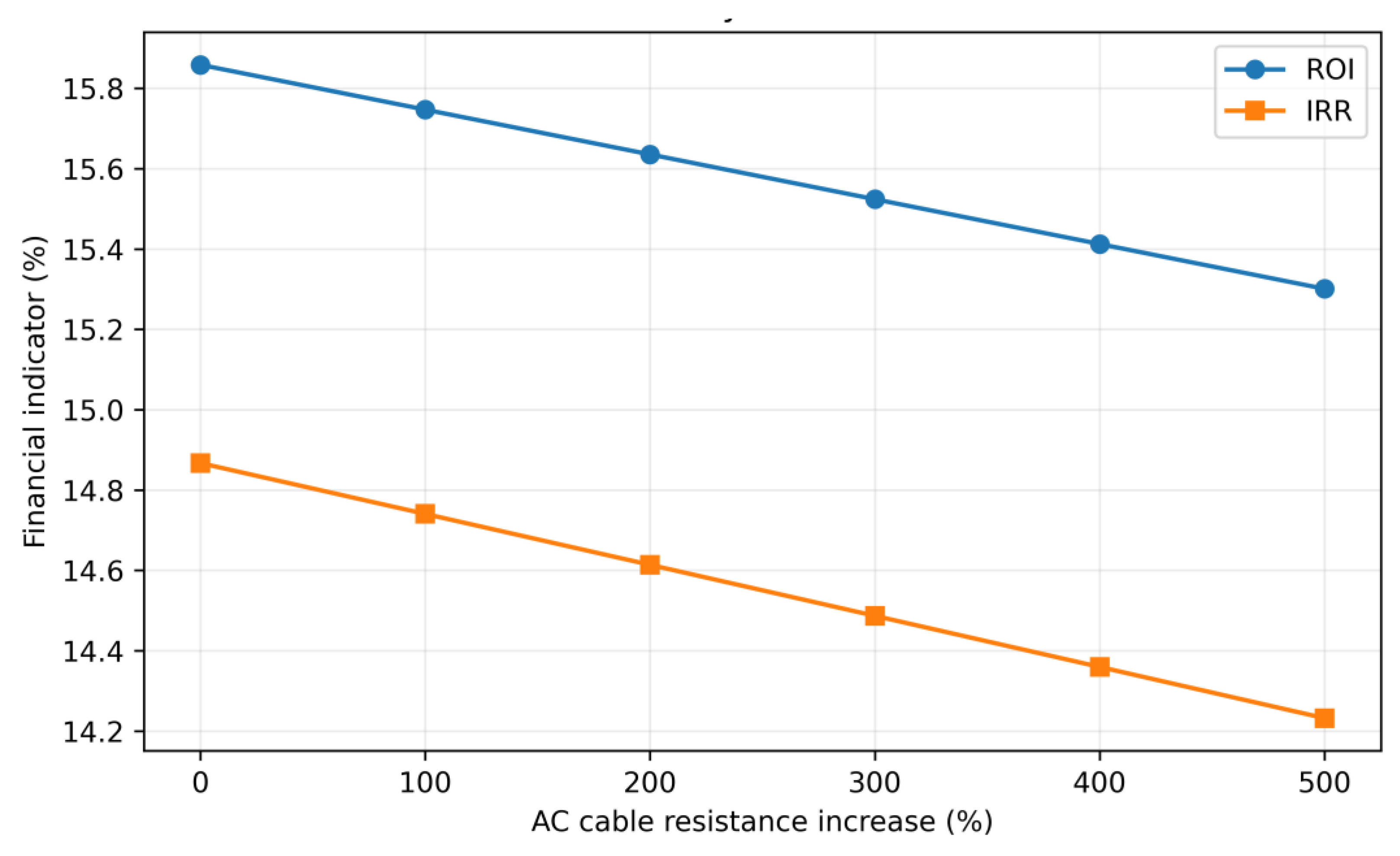
Figure 17.
REPC payback and discounted payback as a function of AC cable resistance increase.
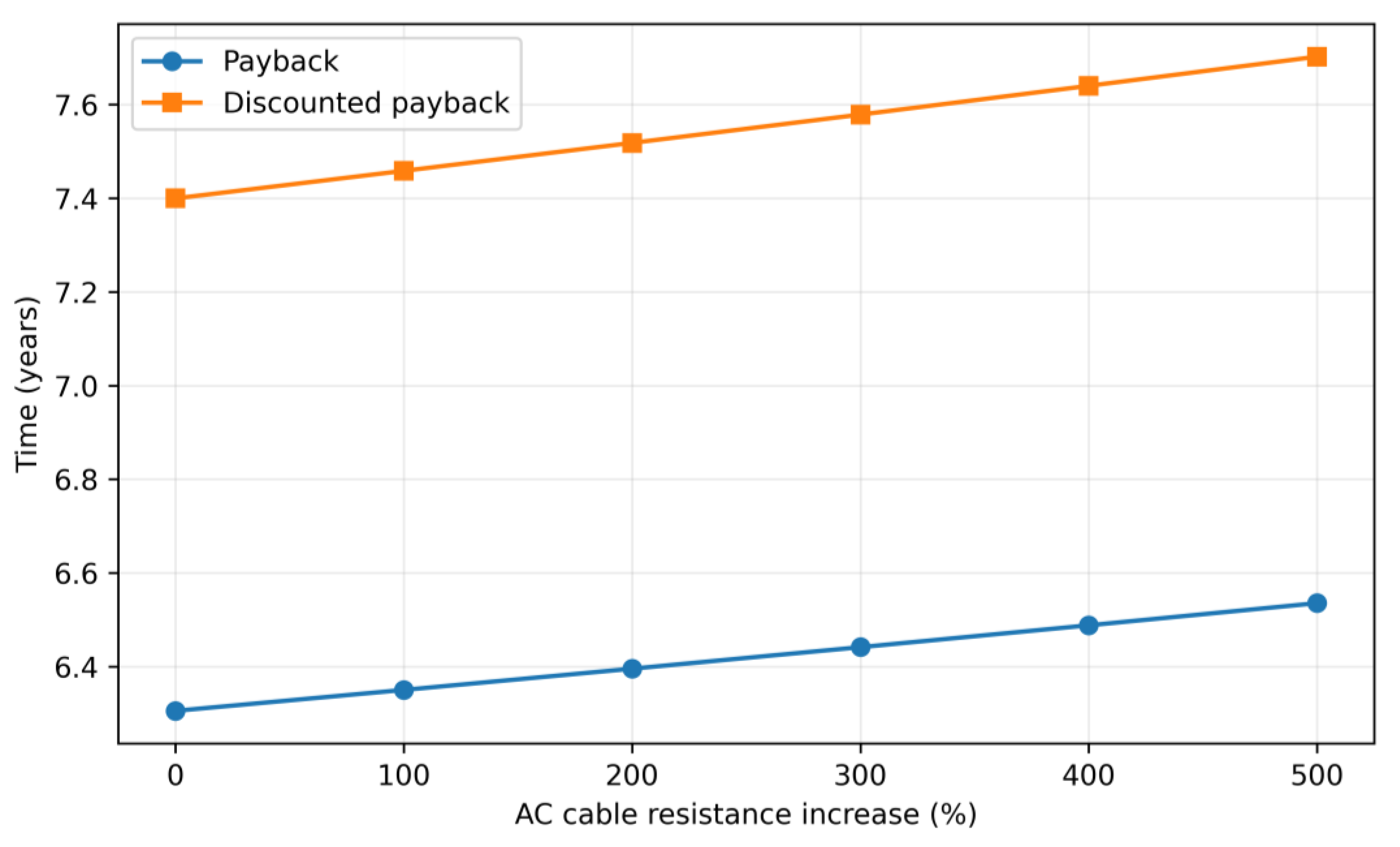
Table IV.
Technical Specifications of the Acciona AW-1500/70 Wind Turbine.
| Parameter | Value | Unit |
| Rated capacity (PR) | 1500 | kW |
| Rotor Diameter (D) | 70 | m |
| Class | IEC IA | - |
| Sweep area | 3848 | m² |
| Power density | 0.38 | kW/m² |
| Number of blades | 3 | - |
| Blade length | 34 | m |
| Maximum rotor speed | 20.2 | rpm |
| Blade material | Epoxy resin | - |
| Power control | Independent pitch for each blade | - |
| Cut-in wind speed (Vcut-in) | 3.0 | m/s |
| Rated wind speed (Vr) | 11.6 | m/s |
| Cut-out wind speed (Vcut-off) | 25.0 | m/s |
| Generator type | DFIG | - |
| Rated voltage (VLL) | 13.8 | kV |
| Grid frequency (f) | 60 | Hz |
| Hub height (hhub) | 60–80 | m |
| Nacelle weight | 52.2–53.2 | TONS |
| Rotor weight | 15.2 | TONS |
| Maximum tower weight | 135 | TONS |
| Total weight | 202.4–202.7 | TONS |
Table V.
Technical Data of Underground Cable Circuits.
| Description |
Circuit 1 |
Circuit 2 |
Unit |
| Number of wind turbines | 2 | 3 | - |
| Rated power (PR) | 3.0 | 4.5 | MW |
| RMS line to line voltage (VLL) | 13.8 | 13.8 | kV |
| Rated current (IR) | 139.5 | 209.2 | A |
| Distance to the electrical substation (SE) | 535.53 | 65.6 | m |
| Total length | 1018.63 | 1031.8 | m |
| Conductor size | 1/0 AWG | 2/0 AWG | - |
| Phase resistance (Rph) | 0.579 | 0.417 | Ω/km |
| Phase inductance (Lph) | 5.60E-04 | 4.69E-04 | H/km |
Table VI.
Design and Environmental Parameters for Underground Cables.
| Description |
Cable 1/0 AWG |
Cable 2/0 AWG |
Unit |
| Operating frequency (f) | 60 | 60 | Hz |
| Number of cables (N) | 3 | 3 | - |
| Number of conductors per cable (Nc) | 2 | 2 | - |
| Geometry |
Cable 1/0 AWG |
Cable 2/0 AWG |
Unit |
| Radius r₁ | 0.0038 | 0.0040 | m |
| Radius r₂ | 0.0083 | 0.00925 | m |
| Radius r₃ | 0.0092 | 0.01025 | m |
| Radius r₄ | 0.0134 | 0.0140 | m |
| Depth h | 1.10 | 1.10 | m |
| Distance x | 0.25 | 0.25 | m |
| Materials |
Cable 1/0 AWG |
Cable 2/0 AWG |
Unit |
| Conductor resistivity (ρc) | 1.72E-8 | 1.72E-8 | Ω-m |
| Sheath resistivity (ρsh) | 1.72E-8 | 1.72E-8 | Ω-m |
| Insulation relative permittivity (εr) | 2.4 | 2.4 | - |
| Insulation relative permeability (μr) | 5 | 5 | - |
| Soil properties |
Cable 1/0 AWG |
Cable 2/0 AWG |
Unit |
| Soil resistivity (ρs) | 100 | 100 | Ω-m |
| Relative permittivity (εs) | 1 | 1 | - |
| Soil loss tangent (tan δ) | 0.001 | 0.001 | - |
Table VII.
Comparative economic results for the AC and DC representations.
| Cash-flow scenario | Model | ROI (%) | IRR (%) | Payback (yr) | Discounted payback (yr) | Economic interpretation | Source |
| Gross results (REPG) | AC | 13.9866 | 11.9605 | 7.1497 | 8.5706 | Gross cash flow | [20] |
| Gross results (REPG) | DC | 13.9866 | 11.9605 | 7.1497 | 8.5706 | Gross cash flow | [20] |
| Net results (REPN) | AC | 13.2895 | 11.8826 | 7.5248 | 9.1273 | After operating costs | [20] |
| Net results (REPN) | DC | 13.2520 | 11.8378 | 7.5460 | 9.1575 | After operating costs | [20] |
| Net + taxes (REPNT) | AC | 10.4353 | 11.8826 | 7.1273 | 9.1575 | Taxes reduce ROI | [20] |
| Net + taxes (REPNT) | DC | 10.4110 | 11.8378 | 7.5460 | 9.1575 | Taxes reduce ROI | [20] |
| CEL revenues (REPC) | AC | 15.9027 | 14.9168 | 6.2883 | 7.3767 | Best financial performance | [20] |
| CEL revenues (REPC) | DC | 15.8587 | 14.8670 | 6.3057 | 7.3996 | Best financial performance | [20] |
| CEL + taxes (REPCT) | AC | 15.9026 | 14.9168 | 6.2883 | 7.3767 | Best financial performance | [20] |
| CEL + taxes (REPCT) | DC | 15.8587 | 14.8670 | 6.3057 | 7.3996 | Best financial performance | [20] |
Table VIII.
Sensitivity of the REPC financial indicators to AC cable resistance.
| Resistance increase (%) | Resistance factor | ROI (%) | IRR (%) | Payback (years) | Discounted payback (years) |
| 0 | 1 | 15.8587 | 14.8670 | 6.3057 | 7.3996 |
| 100 | 2 | 15.7471 | 14.7405 | 6.3504 | 7.4584 |
| 200 | 3 | 15.6356 | 14.6137 | 6.3957 | 7.5180 |
| 300 | 4 | 15.5240 | 14.4867 | 6.4416 | 7.5785 |
| 400 | 5 | 15.4124 | 14.3594 | 6.4883 | 7.6398 |
| 500 | 6 | 15.3008 | 14.2319 | 6.5356 | 7.7021 |
Disclaimer/Publisher’s Note: The statements, opinions and data contained in all publications are solely those of the individual author(s) and contributor(s) and not of MDPI and/or the editor(s). MDPI and/or the editor(s) disclaim responsibility for any injury to people or property resulting from any ideas, methods, instructions or products referred to in the content. |
© 2026 by the authors. Licensee MDPI, Basel, Switzerland. This article is an open access article distributed under the terms and conditions of the Creative Commons Attribution (CC BY) license (http://creativecommons.org/licenses/by/4.0/).
Copyright: This open access article is published under a Creative Commons CC BY 4.0 license, which permit the free download, distribution, and reuse, provided that the author and preprint are cited in any reuse.