

Submitted:
02 September 2026
Posted:
02 September 2026
You are already at the latest version
Abstract
Power flow analysis is fundamental to power system planning, but repeated full network solutions become increasingly computationally demanding as system size and scenario volumes grow with the penetration of distributed energy resources. This paper develops and validates a partitioned power flow framework implemented in PSS®E, treated as a closed commercial solver without access to its internal Jacobian or solver state. The framework comprises three stages: network partitioning, automated case decomposition, and iterative boundary coordination. Spectral clustering based on real power flow, inverse reactance, and Z-bus electrical distance is compared with METIS multilevel graph partitioning, with METIS selected for its computational efficiency, partition balance, and independence from a prior power flow solution. The resulting bus to zone allocation is automatically converted into independently solvable regional cases using virtual reference buses at inter area boundaries. A master–worker scheme then solves the regional cases in parallel and iteratively reconciles duplicated interface voltage variables using an under relaxed boundary consensus update. The framework is validated against the centralised PSS®E Newton–Raphson solution using the IEEE 30-bus, IEEE 300-bus, and 6717-bus Texas synthetic systems. Mean voltage magnitude deviations remain below 0.00042 p.u. across the three systems, while the maximum deviations are 0.00005, 0.00293, and 0.03882 p.u., respectively; the larger Texas system deviations are confined to a small number of buses located predominantly near partition boundaries. Although the partitioned implementation does not provide a wall clock speedup on the four core workstation used in this study, the results demonstrate the feasibility of a fully automated domain-decomposed power flow workflow operating around an unmodified commercial solver and identify the accuracy and computational trade offs associated with boundary-based regional coordination.
Keywords:
distributed power flow
; network decomposition
; boundary consensus
; domain decomposition
; parallel computing
; network partitioning
; METIS
; spectral clustering
; PSS®E
1. Introduction
1.1. Background
Power flow analysis is a foundational tool in power system planning. It determines the steady state voltage at every bus, the loading on every branch, and whether a proposed operating point is feasible at under a specified set of network and operating conditions. Planners rely on it to test network reinforcements, screen contingencies, and assess the integration of new generation, loads, and distributed energy resources. Most other steady state studies take a solved power flow as their starting point. The calculation is therefore repeated extensively across planning, operational, and scenario based studies. Industrial practice relies widely on full network solvers such as Siemens PSS®E. These tools assemble the complete system Jacobian, factorise it, and iterate to a converged solution. The approach is accurate, mature, and well understood. It remains the benchmark against which any alternative must be measured. However, conventional solution workflows are typically monolithic: the complete network model is processed as a single numerical problem for each study condition. Consequently, even when changes are concentrated within a limited part of the system, the global power flow problem is generally resolved in its entirety.
1.2. Motivation
Power flow studies are no longer run one at a time. Distributed energy resources are making the systems that must be modelled more complex [1]. Planning, contingency, and hosting capacity studies now sweep increasingly large sets of operating conditions, contingencies, connection scenarios, and control settings. Everyone of those cases is typically evaluated through a complete network solution. The workload is therefore not only larger than it once was, but also naturally divisible. Network decomposition provides an alternative computational structure in which the original system is divided into electrically connected regions that can be solved separately while exchanging information only at their interfaces. The network is split into zones. Each zone is solved independently in its own process, and the zones iteratively reconcile the voltage variables associated with their shared boundaries. This decomposition has several potential structural advantages. Once regional models have been generated, each worker operates only on its assigned sub-network, and the regional power flow solutions can be executed independently within each coordination iteration. This structure provides a basis for parallel execution and can, in principle, be extended from multi process computation on a single workstation to physically distributed computing environments. The practical benefit, however, depends on the trade-off between reduced regional problem size and the additional computational overhead introduced by case management, interface exchange, and iterative boundary reconciliation.
The obstacle is the solver itself. Distributed power flow formulations in the literature assume access to solver internals, including Jacobian blocks, sensitivities, and iteration state. Industrial practice runs on closed commercial tools that expose none of these. PSS®E is representative: it is driven through a public Python API, its Newton–Raphson engine is compiled inside a binary, and does not expose the Jacobian or internal nonlinear solver state required by many conventional domain decomposition formulations. This creates a practical implementation gap between domain decomposition methods developed in research environments and their use with established commercial power system software. Addressing this gap requires network partitioning, regional case generation, local power flow execution, and boundary reconciliation to operate using only quantities available through the external solver interface. Accordingly, this paper develops and evaluates an automated network-decomposition framework in which PSS®E is treated as an unmodified black box power flow solver. The proposed workflow combines graph based partition allocation, automated construction of independently solvable regional cases, parallel regional Newton–Raphson solutions, and an under relaxed boundary consensus procedure that iteratively reconciles interface voltage variables without requiring access to the solver Jacobian or internal iteration state.
1.3. Organisation
The paper is organised around the three stages of the framework. Section 2 reviews related work and identifies the research gap. Section 3 defines the proposed framework and states the contributions. Section 4 introduces the test systems. Section 5 to Section 7 then present the three stages in turn: the partition allocation study and the selected method, the automated case splitting pipeline, and the parallel boundary consensus coordinator. Section 8 reports the end to end validation of the assembled framework against the centralised solver. It covers convergence behaviour, computational performance, memory requirements, and solution accuracy relative to the centralised Newton–Raphson reference. Section 9 concludes the paper and identifies opportunities for extending the framework to larger systems and distributed computing environments.
The central research question addressed in this work is whether a commercial power flow solver can be embedded within a fully automated domain decomposed workflow without access to its internal Jacobian or nonlinear solver state, while retaining acceptable agreement with the corresponding centralised solution. The study therefore evaluates not only the feasibility of automated decomposition and coordination, but also the resulting trade offs among partition quality, convergence behaviour, computational overhead, and solution accuracy.
2. Literature Review
2.1. Power Flow Analysis and the Cost of Repeated Solutions
The steady state power flow problem and its solution by Newton Raphson iteration are long established and treated definitively in the standard references on load flow analysis [2,3]. The robust numerical characteristics of the method have contributed to its widespread use in commercial tools such as Siemens PSS®E [4], supported by the optimally ordered sparse factorisation techniques that keep each iteration computationally feasible on large networks [5] and by approximate variants such as fast decoupled load flow, which trade some modelling fidelity and convergence robustness for speed [6]. vThe cost of a centralised solve is nevertheless influenced by the size, sparsity, and conditioning of the global system equations, and the complete network solution is generally repeated for each operating scenario [3,7].
The rapid penetration of distributed energy resources (DERs) has increased the number and diversity of operating conditions that must be assessed. Rooftop solar already supplies more than ten percent of Australia’s electricity [8], and connection volumes continue to grow [9], so operators must screen increasing numbers of candidate scenarios for planning, contingency, and hosting capacity studies. Reviews of high performance computing applied to power flow analysis identify the linear system solve as a major computational component of power flow analysis [1]; When repeated across large scenario sets, this motivates investigation of alternative computational structures that can exploit parallelism or regional decomposition. Interest has therefore shifted towards distributed and partitioned formulations, in which the network is divided into independently solvable zones whose shared boundaries are iteratively reconciled to recover a network wide solution.
2.2. Network Partitioning of Power Systems
Decomposing a large network into separately solvable pieces predates modern parallel hardware. Kron’s diakoptics established the principle that a large system may be solved piecewise provided the interconnection variables are correctly accounted for [10], and the same idea underpins modern domain decomposition treatments of sparse linear systems [11]. Contemporary work recasts the task as graph partitioning, where partition quality strongly influences the computational characteristics of the resulting regional solution: few tie lines reduce the boundary information that must be exchanged, and zones of similar size distribute work evenly. Because a parallel solver is affected by workload imbalance between zones, both properties matter.
Spectral clustering is a widely used family of methods family in power system studies, applied to controlled islanding, voltage zone identification, and decomposition for distributed computation. The approach rests on the graph Laplacian, whose low order eigenvectors expose the dominant connectivity structure of the network [12,13]. Its objective often formulated through spectral relaxations of graph cut objectives such as the normalised cut introduced by Shi and Malik [14], which scores a partition by the cut weight between zones relative to the volume of each zone and so avoids the degenerate solutions a raw minimum cut admits; the earlier spectral ratio cut method of Hagen and Kahng addresses the same degeneracy in circuit partitioning [15], and guarantees for spectral partitioning have been established on structured graphs such as planar graphs and finite element meshes [16]. What distinguishes applications is the edge weight. Weighting branches by real power flow treats heavily loaded corridors as strongly coupled [17,18], whereas parameter based weights such as inverse reactance or impedance derived electrical distance avoid any dependence on the operating point [19,20]. Sensitivity based electrical distance has a long history in secondary voltage control zoning [21] and remains the subject of comparative study [22]. The recognised weakness of the family is that good electrical separation does not necessarily guarantee balanced region sizes. Depending on the graph weighting and clustering procedure, the resulting partitions may contain significantly different numbers of buses, which can reduce computational balance in a parallel implementation [12].
Multilevel graph partitioning approaches the same problem from the combinatorial side. The scheme coarsens the graph through successive vertex matchings, partitions the smallest graph directly, and then projects the partition back while refining it at each level [23,24]; the refinement step derives from the Kernighan–Lin boundary exchange heuristic [25] and its linear time reformulation by Fiduccia and Mattheyses [26]. Because multilevel approaches can explicitly constrain partition balance while reducing edge cuts, the resulting regions can be better suited to parallel workloads where similar regional problem sizes are desirable. The method runs in near linear time using topology alone, and METIS has consequently become a widely used tool for decomposing large sparse graphs in parallel scientific computing [24].
Partition quality is assessed with solver independent graph measures. Newman modularity compares intra zone connectivity against a degree preserving random graph [27] and is standard in the wider community detection literature [28], while the normalised cut and the tie line count capture boundary size and inter regional coupling. Network partitioning also remains active for goals that share these tools but differ in objective, including the coordination of networked microgrids [29], constrained k-way normalised cut formulations [30], and the aggregation of distribution grid flexibility [31]. That work confirms the maturity and breadth of partitioning, but also illustrates that the preferred partition depends strongly on the downstream application. In the present work, the partition must balance electrical separation, regional size, and the number of interfaces that must subsequently be reconciled during the distributed power flow solution.
2.3. Distributed Power Flow Coordination and Boundary Reconciliation
Once a network is partitioned, the zones must be brought into agreement on their shared boundary variables. Surveys of distributed optimisation and control for electric power systems catalogue the available coordination schemes and, importantly, the information each one requires from its sub solvers [32]. The Alternating Direction Method of Multipliers established approach for coordinating decomposed optimisation problems [33], with its convergence behaviour characterised both classically [34] and through more recent continuous time analyses [35]. Within power systems it has been applied to optimal power flow [36,37], to distributed OPF for microgrids [38], and to state estimation, demand response, and market coordination [39]. Parallel and asynchronous variants relax the global synchronisation barrier in order to exploit multi core hardware [40,41], learning based schemes have been proposed to accelerate convergence [42], and related decomposition methods such as ALADIN provide alternative distributed optimisation strategies at the cost of requiring derivative information from each sub solver [43]. These methods provide important context for distributed coordination; however, their information requirements are not necessarily compatible with a commercial power flow solver treated as a numerical black box. In particular, conventional ADMM and related optimisation based decomposition methods are formulated around explicit local optimisation variables, consensus constraints, penalty terms, and, in many cases, derivative or dual variable information. The problem addressed in this work is different in that each regional subproblem is solved directly using the existing PSS®E Newton–Raphson power flow engine. The coordinator has access to solved network quantities through the public API but does not access the internal Jacobian, sensitivities, or nonlinear solver state. Coordination must therefore be performed through externally accessible interface quantities. Accordingly, the framework developed here uses virtual boundary reference buses and iteratively updates their setpoints through an under relaxed boundary consensus procedure. The regional power flow problems remain independent Newton–Raphson solutions, while the outer coordination process drives their interface voltage variables towards consistency. The method is therefore more appropriately characterised as a relaxed boundary reconciliation or domain decomposition procedure rather than a conventional ADMM optimisation algorithm. Section 7 develops this coordination procedure in detail.
2.4. Parallel and High Performance Power Flow Computation
A parallel literature addresses the acceleration of power flow, OPF, and dynamic simulation through multi core and distributed computation, including domain decomposition of the network equations and the distribution of independent cases across processors; representative work demonstrates parallel processing of combined transmission–distribution dynamic simulation [44]. Of particular relevance here, recent studies have examined how the choice of grid partitioning algorithm affects combined distributed AC optimal power flow and parallel power grid simulation, confirming that partition quality and the resulting coordination overhead materially shape the achievable computational performance [45]. This body of work establishes both the opportunity, since modern planning workloads are highly parallelisable, and the obstacles, chiefly coordination overhead and the memory duplication incurred when each worker holds an independent copy of the solver and its data. Decomposition therefore does not inherently guarantee a wall clock speed up. Process creation, case loading, synchronisation, boundary exchange, and repeated regional solver calls introduce additional overhead that must be offset by the computational benefit of smaller regional problems. Classical parallel computing bounds provide a useful interpretation: the serial fraction of a workload limits the attainable speed up for a fixed problem size[46], while the achievable benefit can increase when problem size and available parallel resources are scaled together [47].
A further practical consideration arises when the underlying commercial solver requires each worker to initialise a separate software instance. Although each worker may contain only a regional network case, solver runtime and process level data structures can be replicated across workers. Consequently, memory use and process management overhead must be considered alongside solution time when evaluating the practical value of a distributed implementation. For this reason, the framework developed in this paper is evaluated not only in terms of solution accuracy, but also with respect to convergence behaviour, wall clock execution time, CPU utilisation, and memory requirements.
2.5. Research Gap
Almost all of the work above is implemented either in open research codes such as MATPOWER [48] or in purpose written prototypes, and is evaluated on openly available benchmark archives [49] and on synthetic networks constructed to reproduce the structural characteristics of real systems [50]. Many such research environments provide direct access to the mathematical representation of the network equations and allow customised access to solver variables, Jacobians, sensitivities, or algorithmic states. This flexibility enables decomposition strategies that are considerably more difficult to reproduce when the power flow engine is embedded within closed commercial software. Closed commercial tools such as PSS®E expose a more restricted external interface, and additionally the internal Newton–Raphson Jacobian and nonlinear iteration state are not exposed through the standard public API. Despite the maturity of both network partitioning and distributed coordination methods, it therefore remains unclear how an end to end automated network decomposition workflow can be constructed around such a solver using only externally accessible quantities, and what accuracy and computational trade offs result from this constraint.
The research gap addressed in this paper is therefore not the development of a new power flow engine or a new graph partitioning algorithm. Rather, it is the development and validation of an automated domain decomposed power flow workflow that uses an unmodified commercial Newton–Raphson solver for each regional problem while coordinating those problems exclusively through quantities available from the public solver interface. Specifically, the study investigates whether:
- 1.
- a full PSS®E network can be automatically partitioned and transformed into independently solvable regional cases;
- 2.
- the resulting regional solutions can be reconciled through relaxed boundary voltage consensus without access to the global or regional solver Jacobians; and
- 3.
- the assembled framework can maintain acceptable agreement with the centralised reference solution while revealing the associated trade offs in partition balance, interface size, convergence, execution time, and memory usage.
These questions define the technical scope of the framework presented in the following sections.
3. Proposed Framework
The framework proposed here addresses the gap identified above by assembling a complete partitioned power flow workflow on top of an unmodified commercial solver. Its governing constraint is that PSS®E is treated strictly as a black box: it is driven only through its public Python API, no internal solver data is requested, and no attempt is made to alter or replace its Newton Raphson engine. The resulting framework is therefore designed around quantities that can be accessed or modified externally, principally network topology, bus and branch data, regional case files, and solved bus voltage quantities. This constraint distinguishes the proposed implementation from decomposition methods that require direct manipulation of Jacobian blocks, derivative information, or internal nonlinear solver states.
The workflow is organised as three sequential stages that together carry a single monolithic case file through to coordinated regional power flow solution.
- 1.
- Network partition allocation: The bus branch topology of the master case is treated as a graph and divided into k zones. Because the allocation fixes both the distribution of network buses across regional workers and the volume of boundary data that must later be exchanged, it is treated as an explicit selection stage rather than a fixed choice: Four candidate partitioning approaches—real power flow weighted spectral clustering, inverse reactance weighted spectral clustering, Z-bus electrical distance clustering, and METIS multilevel graph partitioning—are implemented under a common workflow and compared using consistent graph based metrics. The selected allocation is subsequently passed to the automated case generation stage.
- 2.
- Automated case splitting: The abstract bus to zone map is realised as k structurally complete PSS®E cases, each solvable in isolation. Inter regional connections are identified and represented within each regional case through virtual boundary reference buses. These buses provide externally controllable voltage boundary conditions that represent the electrical influence of the neighbouring regions omitted from the local model. The resulting regional cases preserve their internal network topology while exposing the interface quantities required by the coordination stage.
- 3.
- Parallel boundary consensus coordination: A master coordinator dispatches the regional cases to a pool of worker processes, each hosting its own PSS®E instance, and coordinates the regional solutions through iterative exchange of their boundary voltage quantities. During each outer coordination iteration, the regional cases are solved independently using the PSS®E Newton–Raphson engine. The solved interface voltages are returned to the master process and used to update the corresponding virtual boundary conditions through an under relaxed consensus rule. The process is repeated until the mismatch between duplicated interface voltage representations satisfies a specified convergence tolerance. Importantly, the coordination procedure operates outside the PSS®E power flow engine and does not modify its local Newton–Raphson formulation. It therefore acts as an outer domain decomposition layer around a set of conventional regional power flow solutions.
The contributions are correspondingly threefold. First, the study provides a consistent comparison of four network partitioning approaches flow weighted, reactance weighted, electrical distance, and multilevel graph partitioning across test systems ranging from 30 to 6717 buses. The comparison evaluates partition balance, interface size, graph separation, and computational cost using metrics that are independent of the downstream power flow solver. Second, an automated case decomposition pipeline is developed to transform a full PSS®E network model into independently solvable regional cases while retaining controllable electrical representations at the inter regional boundaries. This demonstrates that regional power flow models can be generated programmatically around an unmodified commercial solver. Third, a relaxed boundary consensus coordinator is developed that requires only quantities available through the public PSS®E interface. The framework therefore demonstrates that multiple independent commercial solver instances can be coordinated without access to their Jacobians or internal nonlinear iteration states, while permitting the resulting regional solution to be quantitatively compared against the corresponding centralised Newton–Raphson reference.
The scope of the claims made in this study is deliberately limited. The primary objective is to establish the technical feasibility of the complete decomposition and coordination workflow and to quantify its agreement with the centralised reference solution. Computational behaviour is reported as a secondary observation, and because the experiments run on a single workstation whose core count is smaller than the zone count of the larger cases, no wall clock speed up is claimed. The computational results are therefore interpreted as an assessment of implementation behaviour rather than as evidence of parallel acceleration. The present contribution lies primarily in the automated architecture: partition allocation, regional model generation, independent commercial solver execution, and iterative boundary reconciliation are integrated into a single reproducible workflow. The accuracy, convergence, timing, and memory characteristics of this architecture are evaluated in Section 8.
4. Test Systems
Three standard systems were used throughout the study, chosen to span a broad range of network sizes and to evaluate the behaviour of the proposed framework from small benchmark systems to an interconnection-scale synthetic network. Each system is partitioned into k zones, where k is the only user supplied parameter of the partitioning stage. It fixes the number of standalone regional cases the splitter produces, and therefore the number of independent local solves the coordinator dispatches in every outer iteration; the average zone therefore contains roughly of the system’s n buses. Increasing k generally reduces the size of each regional subproblem but can also increase the number of inter regional boundaries that must be reconciled during the coordination process. The selected values of k were therefore increased with network size to provide multiple regional subproblems while retaining a manageable number of interfaces for the present validation study. A systematic optimisation of k is outside the scope of this work and is identified as an area for future investigation. Table 1 summarises the test systems and the partition counts used in the experiments.
5. Stage 1: Network Partition Allocation
The boundary consensus coordination framework is flexible regarding how buses are assigned to zones, but that assignment directly influences the computational characteristics of the subsequent regional solution: balanced zones reduce workload imbalance between workers, and few tie lines reduce the number of inter regional interfaces that must be represented and reconciled. Network partition allocation is therefore treated here as an explicit pre processing and method selection stage. Four candidate methods were implemented behind a common interface and run under identical conditions on the test systems to compare their balance, separation quality, interface size, and computational requirements before selecting one method for the downstream decomposition workflow.
5.1. Candidate Methods
Three of the four candidates are spectral methods sharing a common core. Each builds a weighted graph whose vertices are buses and whose edges are branches, constructs a graph Laplacian from the weighted adjacency matrix W and corresponding degree matrix D , and uses a low dimensional spectral embedding to represent the dominant connectivity structure of the network. The embedded bus representations are subsequently grouped into k zones using the same clustering procedure for all three spectral variants, so that their principal difference is the definition of electrical coupling assigned to each graph edge. The partitioning objective is related to spectral graph cut formulations such as the normalised cut [14],
so every spectral variant aims to group electrically well connected buses into the same zone while keeping inter zone coupling comparatively small. What distinguishes the three is only the edge weight , that is, the definition of electrical closeness [12,19].
The MW flow method defines as the magnitude of real power flow on branch under a solved base case operating point. The underlying idea is that heavily loaded corridors are strongly coupled and should remain within the same zone. Its main limitation is that, because the flow pattern depends on the operating point, the resulting partition can changes with dispatch and loading conditions. As a result, a solved base case power flow solution is required before partitioning can be performed.
The other two spectral methods are parameter based and do not require a prior power flow solution. The method assigns each branch a weight equal to the inverse magnitude of its series reactance, so lines with small series reactance indicate strong electrical coupling and tend to keep buses together in the same zone. Because the weighting is derived from branch parameters rather than a solved power flow state, the resulting graph is independent of the particular active power dispatch used in the MW weighted method. The Z-bus method takes a more global electrical view by defining the distance between buses as
where Z is the Moore–Penrose pseudo inverse of the bus admittance matrix Y. The resulting impedance-derived distance provides a system-level measure of electrical separation and is related to electrical-distance measures used in voltage-control zoning and network aggregation. However, directly clustering the raw Z-bus distance can isolate the radial busses. To address this, the implementation clusters a restricted topology graph whose edges are weighted by , combining electrical distance with structural connectivity. The main computational cost arises from computing the pseudo inverse, a dense operation of complexity in standard direct implementations [11], which becomes significant for large systems. All electrical distance calculations are performed on a common per-unit network representation before the resulting weights are mapped to the topology restricted graph.
The METIS method differs from the spectral methods, partitioning by multilevel refinement in three phases. A coarsening phase repeatedly collapses matched vertex pairs to build a sequence of progressively smaller graphs; the coarsest graph is partitioned directly; and an uncoarsening phase projects the partition back level by level, applying a Kernighan–Lin/Fiduccia–Mattheyses style boundary search to refine it at each step [25,26]. A hard balance constraint holds every zone near vertices while the refinement minimises the edge cut. The multilevel partitioning procedure explicitly favours balanced vertex counts while reducing the edge cut, making it suitable for parallel workloads in which substantial differences in regional size can create worker imbalance. METIS uses only the unweighted network topology in the implementation considered here no power flow and no admittance matrix are needed and runs in near linear time, which is why it is widely used for partitioning large graphs in parallel scientific computing [23,24]. Table 2 summarises the four configurations.
5.2. METIS Implementation
Producing the METIS allocation requires a topology reader and the METIS bindings: Python 3.9+ with pymetis, the Python interface to the METIS C library, installable from conda forge or pip together with networkx, NumPy, SciPy and pandas. No PSS®E license, power flow solution, or admittance matrix is required at this stage. Given a PSS®E RAW case and a zone count k, the procedure returns a bus to zone allocation (Table 3).
The method depends only on the case file and the assigned number of zones k. First, the RAW file is parsed to extract the bus and branch lists. An undirected, unweighted graph is then constructed, with parallel branches merged into a single edge and self loops removed. Bus identifiers are relabelled to contiguous 0-based indices and converted into the adjacency list format required by METIS. The graph is partitioned using pymetis.part_graph, which performs multilevel coarsening, partitioning, and refinement using the configured METIS partitioning options. Finally, a connectivity repair step reassigns disconnected components to neighbouring zones until every zone forms a single connected component, preventing disconnected regional islands before downstream case generation. Topological connectivity alone does not mathematically guarantee non singularity or Newton–Raphson convergence; the solvability of every generated regional case is therefore verified separately during Stage 2. The resulting partition is written as a simple (BusID, ZoneID) table for the Stage 2 network splitter.
5.3. Evaluation Metrics
Partitions are scored on solver independent measures computed on the common network topology so that the candidate methods can be compared on a consistent basis. Separation quality is captured by Newman modularity [27],where larger values indicate stronger concentration of connections within zones relative to intra zone connectivity with that of a degree preserving random graph, and by the normalised cut value, in which lower is better. Boundary size is captured by the tie line count the number of branches whose endpoints lie in different zones and by the number of buses incident on those inter zone connections. Balance is captured by the size coefficient of variation, of the zone sizes, so closer to 0 is better. A connectedness check requires exactly one connected component per zone, and the wall clock runtime of the partitioning step is recorded.
5.4. Comparison Results
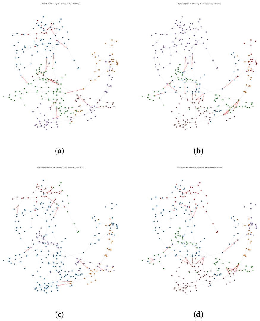
The quantitative comparison of the four methods across the three test systems is given in Table 4, and the corresponding allocation maps are shown in Figure 1 Figure 3.
The identical comparison was conducted on the larger IEEE 300 bus system, where the disparities between approaches were more pronounced (Figure 2). The Spectral MW approach yielded a less equitable split, whereas METIS preserved a more appropriate zone configuration for parallel computation.
Figure 2.
Partition allocation maps for the IEEE 300-bus system, : (a) METIS; (b) Spectral ; (c) Spectral MW; (d) Z-bus distance.
Figure 2.
Partition allocation maps for the IEEE 300-bus system, : (a) METIS; (b) Spectral ; (c) Spectral MW; (d) Z-bus distance.
The partitioning approaches were finally applied to the Texas 7k synthetic grid to evaluate performance at the interconnection scale (Figure 3).
Table 4 summarises the performance of the four partitioning methods across the three test systems. For the IEEE 30-bus system, the four approaches do not produce a single dominant solution. The spectral method yields the lowest size CoV and the highest modularity, whereas the Z-bus method produces the fewest tie lines and lowest NCut. METIS provides the lowest partitioning runtime but does not outperform the spectral approaches on all graph quality measures. The methods diverge as the network grows.
On the IEEE 300 bus system, METIS provides the lowest size imbalance, the highest modularity, and the lowest NCut among the four methods while retaining a comparatively small number of tielines. The MW weighted spectral method produces only 15 inter zone branches, but this occurs together with a highly unbalanced allocation in which approximately 59% of the buses are assigned to a single zone. The result illustrates why tie line count should not be interpreted independently of regional balance.
At the 6717 bus scale, a clear trade off emerges between regional balance and interface size. METIS produces the most balanced allocation, with the largest zone containing 17.1% of the buses, and completes the partitioning stage in approximately 3.2 s. However, it also produces 579 tie lines and the highest NCut of the four methods. In contrast, the spectral and Z-bus approaches produce fewer inter zone connections and lower NCut values, but with substantially greater region size imbalance and longer partitioning times. The Z-bus implementation requires approximately 312 s because of the computational cost associated with constructing the dense electricald istance representation. Modularity remains broadly comparable among the better performing partitions. For the downstream experiments in this study, three properties were prioritised: regional size balance, low partition generation cost, and independence from a previously solved operating point. On these criteria, METIS provides the most suitable allocation at the largest network scale, although this advantage is obtained at the expense of a larger inter regional interface. METIS is therefore selected as the default partitioning method for Stages 2 and 3. This selection should not be interpreted as demonstrating that METIS is universally optimal; rather, it reflects the priorities of the present parallel regional power flow implementation. Table 5 shows the resulting allocation file from the study. The comparison therefore shows that no single partitioning method dominates all metrics. Spectral and electrical distance approaches can produce smaller interfaces, whereas METIS provides substantially stronger regional balance and lower partition generation time at the largest tested scale. Because the subsequent master–worker implementation is sensitive to worker imbalance and because the selected partition must be generated without requiring a prior solved operating point, METIS is adopted for the remainder of the study. The impact of its larger interface size is evaluated implicitly through the convergence and computational results reported in Section 8.
6. Stage 2: Automated Case Splitting
The selected allocation is an abstract bus to zone map; before it can be used, each zone must be realised as a self contained PSS®E case that can be solved in isolation. An automated case generation pipeline takes the allocation map A produced in Stage 1 and converts the original network into k regional PSS®E cases. The decomposition is performed through three main steps: identification of inter-regional connections, extraction of the regional network topology, and construction of controllable boundary representations for the omitted neighbouring regions.
6.1. Decomposition Procedure
Boundary tie line identification. The pipeline first sweeps every branch in the master case and isolates the tie-lines whose terminals fall in different zones,
where is the global edge set and the circuit identifier.
The resulting set defines the inter-regional electrical interfaces used in the subsequent case-generation and coordination stages. For each inter-regional connection, the terminal buses associated with the two participating regions are recorded together with the corresponding circuit identifier so that the physical interface can be reconstructed consistently within the regional cases.
Topological subsystem extraction: For each zone Z, a clean copy of the master case is loaded into memory and every branch whose two terminals both lie outside Z network elements that do not belong to the regional representation are removed according to the bus-to-zone allocation. The purpose of this operation is to retain the internal topology of the assigned region while removing network elements that are not required for its standalone solution. Inter-regional connections identified in the preceding step are treated separately so that their electrical influence can be represented through controllable boundary conditions rather than through the complete neighbouring network. For each cut connection, the electrical parameters of the original branch are retained in the regional representation, while the remote terminal is represented by a controllable boundary bus whose voltage is supplied by the coordination layer.
Virtual boundary slack conversion: To let each severed sub network resolve its internal nonlinear equations while preserving the electrical rigidity imposed by its omitted neighbours, every boundary bus is converted into a regulated reference through a three part API sequence:
- 1.
- the bus is registered as a generation plant;
- 2.
- a virtual machine of nominal active capacity p.u. is instantiated at it;
- 3.
- its type is reclassified to a regulated Type 3 slack bus.
Within the regional power-flow solution, the virtual reference provides a controllable voltage magnitude and angle at the interface. These setpoints are updated externally by the coordination layer and therefore provide the mechanism through which neighbouring regional solutions influence one another without requiring either region to contain the complete external network. Each zone is then exported as a structurally complete standalone case (Zone_Z.raw). Where a region contains multiple interfaces, each virtual boundary reference is configured according to the PSS®E treatment used in the implementation, while preserving a valid regional power-flow reference structure. The complete pipeline is shown in Figure 4.
6.2. Output and Validation
The pipeline outputs one standalone case per zone, each loadable and solvable independently in PSS®E (Figure 5). The splitter processes the inter-regional connections identified from the allocation map and exports one regional case for each zone. Successful loading and convergence of every generated case in PSS®E verify that the automated decomposition pipeline produces executable regional power-flow models from the original network allocation. The connectivity constraint enforced during Stage 1 is retained during regional case generation, preventing disconnected internal bus groups from being introduced by the partitioning process. However, connectivity alone does not guarantee numerical power flow solvability; consequently, each exported regional case is independently loaded and solved in PSS®E as an explicit validation step before being passed to the Stage 3 coordinator.
Two levels of validation are relevant to the decomposition stage. The first is structural validation, which verifies that all original buses assigned to a region are retained, each regional case remains internally connected, and all intended inter regional interfaces are represented. The second is electrical validation, which determines whether the regional cases reproduce the expected internal solution when supplied with boundary conditions obtained from the centralised reference case. The present workflow performs the structural and standalone solvability checks automatically; the agreement of the fully coordinated regional solution with the centralised solution is subsequently evaluated in Section 8.
7. Stage 3: Parallel Relaxed Boundary Consensus Coordination
7.1. Selection of the Coordination Method
The regional cases must be reconciled so that, at convergence, the zones agree on their shared boundary voltages and together reproduce the global solution. Domain decomposition methods provide this coordination by solving the sub problems locally and exchanging boundary variables iteratively [44], but the choice among them is tightly constrained by the closed PSS®E API, which exposes solved bus voltage arrays yet no internal solver data. Each candidate family was assessed against this constraint.
Schur complement decomposition provides a well-established approach to reducing coupled network equations to an interface problem, but it requires direct access to the sub domain Jacobian blocks in order to form the reduced interface system [11,44]; in PSS®E the Jacobian is compiled within a Fortran binary and is not exposed through the public API, rendering this approach infeasible. ALADIN provides an alternative distributed optimisation framework with strong local coordination properties, but it requires each sub solver to supply gradient, Hessian, and constraint Jacobian information [43], which the API likewise does not provide; constructing these by finite differences would demand several additional perturbed solves per zone per iteration, negating the parallel benefit. Gauss–Seidel style decompositions, in which zones are updated sequentially using the latest neighbouring values, are simple but inherently serial and therefore forfeit the concurrency the framework is designed to exploit. Synchronous Formal ADMM-based coordination provides another important class of distributed methods; however, conventional ADMM formulations require an explicit separable optimisation or feasibility formulation together with consensus and dual variable updates [40],The present implementation instead retains PSS®E as an unchanged nonlinear power flow solver and coordinates only externally accessible boundary quantities.
On this basis, a parallel relaxed boundary-consensus procedure is adopted as the coordination layer of the proposed framework. Boundary voltages are mirrored as virtual boundary reference buses at each cut interface, and the master requires only the boundary voltage magnitude and angle arrays from each worker, quantities that are directly accessible through the public API, with no need for Jacobian or sensitivity data [39,41]. No Jacobian, derivative, or internal Newton–Raphson iteration information is required. Each PSS®E instance is therefore treated as an independent black-box regional solver whose interface with the coordinator is limited to externally specified boundary conditions and solved boundary-voltage quantities. Each PSS®E instance is thereby treated as a black box solver, interfaced solely through its public API and a controlled shared memory buffer.
7.2. Parallel Coordination Procedure
The master coordinator drives a multiprocessing pool toward a globally consistent solution, as illustrated in Figure 6. It launches one worker process per zone, so the pool size equals the zone count k. On the four core workstation used here, at most four workers execute concurrently; for the remaining zones queue and are processed in successive waves. To maintain strict isolation, each worker initialises a standalone PSS®E instance in its own process memory, with logging suppressed to remove terminal I/O latency. On each outer iteration, every worker loads loads the corresponding regional case; updates the virtual boundary-reference setpoints using the current interface values supplied by the master; executes a local Newton–Raphson power-flow solution; and returns the solved voltage magnitude and phase-angle quantities associated with the relevant interface buses. Regional power-flow solutions within the same outer iteration are independent and can therefore be executed in parallel subject to the number of available processor cores. The outer coordination iteration advances only after the required regional boundary results have been collected.
where the under relaxation factor was selected empirically. Under relaxation of this form corresponds to in the standard relaxed ADMM parameterisation [33], and suppresses numerical oscillations at tightly coupled boundaries without requiring adaptive penalty tuning. The loop repeats until the global boundary primal residual satisfies the maximum norm termination criterion
across all inter zone interfaces, after which the master terminates the workers and records the resident memory footprint and iteration count. In the implementation, the boundary state contains the voltage quantities required to initialise the virtual reference associated with each cut interface. Voltage magnitude and phase angle are mapped between corresponding physical and virtual boundary representations before the next regional solution is initiated.
8. Results and Discussion
The performance of the partitioned boundary-consensus framework was evaluated in comparison to the centralised PSS®E Newton Raphson solver across four dimensions: convergence characteristics, wall clock execution duration and CPU usage, memory usage, and solution precision. All tests were initiated from a consistent initialisation procedure and executed on a single multi core workstation, with 3, 6, and 12 worker processes allocated to the IEEE 30 bus, IEEE 300 bus, and Texas 7k systems, respectively. The hardware and software configuration used for all experiments was fixed across the centralised and decomposed cases.
Because Stage 1 operates on network topology alone, the partitioning study was run independently of PSS®E. Both the centralised reference solution and the decomposed framework were run on this same configuration.
| physical/logical cores: | 4 cores |
| Memory | 8 GB RAM |
| Operating system | Windows 11 (64-bit) |
| Power-flow solver | PSS®E 35.6 |
| Solver scripting | Python 3.9 (bundled with PSS®E, psspy interface) |
| Partitioning | Python 3.14 (pymetis, NetworkX, NumPy, SciPy, pandas) |
8.1. Benchmarking Setup
Both methods were tested on the same network cases and workstation, with ten repeated runs for each test. All cases were solved to convergence. The comparison uses two metrics that can be measured consistently for both the centralised and partitioned solvers: the number of solver iterations and the change in memory usage during the solve. The iteration counts are not directly comparable in absolute terms, since a Newton-Raphson iteration and an outer consensus iteration represent different units of work. However, their trends as the system size increases are still useful for comparison.
8.2. Convergence Behaviour
The centralised PSS®E solver achieved convergence in 3, 6, and 210 iterations for the IEEE 30 bus, IEEE 300 bus, and Texas 7k systems, respectively, whereas the partitioned relaxed boundary-consensus coordinator converged in 16, 17, and 17 outer consensus iterations for the same three systems (Table 6). The large increase in the reported centralised iteration count for the Texas 7k case should be interpreted cautiously. Newton–Raphson iteration count is influenced by network conditioning, initialisation, solver configuration, control actions, and convergence settings and is not determined by network size alone. Accordingly, the 210-iteration result is reported as an observed solver outcome rather than as evidence of a general scaling relationship. In contrast, the observed boundary consensus iteration count remained between 16 and 17 across the three tested cases. This result indicates that the number of outer coordination iterations did not increase materially for the particular systems, partitions, initial conditions, relaxation factor, and convergence tolerance considered here. It should not, however, be interpreted as demonstrating scale-independent convergence, because only three network sizes and one partition count per system were evaluated. Each outer boundary-consensus iteration contains multiple local Newton–Raphson solutions and an interface update, whereas a centralised Newton–Raphson iteration represents one global nonlinear update. The iteration counts should therefore be interpreted only within their respective algorithms.
8.3. Wall Clock Time and CPU Utilisation
In terms of wall clock time, the centralised PSS®E solver was more efficient across all three systems (Table 7). The difference was especially evident in the smaller systems, where the centralised solution finished significantly faster, while the decomposed framework’s process management, file loading, and boundary exchange added overhead that made up a larger part of the total runtime. In the Texas 7k system, the relative gap decreased: the centralised solver required 1.521 s, compared to 4.665 s for the partitioned framework, indicating a reduced ratio relative to the 30 and 300 bus scenarios. The total CPU time for the partitioned framework (11.844 s on Texas 7k) surpassed its wall clock time (4.665 s), indicating authentic concurrent multi core execution. This ratio must, however, be read against the available hardware. The workstation provided four CPU cores, so the twelve zone solves of the Texas 7k case could not run simultaneously and were instead processed in three successive waves. Across the three systems the ratio of total CPU time to wall clock time rises from 1.34 to 1.68 to 2.54 as the zone count rises from 3 to 6 to 12, remaining below the four fold ceiling the hardware permits. The absence of a wall clock speed up therefore reflects both the fixed per iterationThe absence of a wall-clock speed-up is therefore consistent with the combined effects of process and file-management overhead, repeated regional solver initialisation, boundary coordination, and the limited number of simultaneously available cores. These results should consequently be interpreted as an implementation and feasibility benchmark rather than as evidence of parallel scaling or computational acceleration [46].
8.4. Memory Results
The centralised solver utilised around 112–117 MiB across the three platforms. The Partitioned framework exhibited significantly higher peak memory, measuring 453.8 MiB, 566.0 MiB, and 569.2 MiB for the 30 bus, 300 bus, and Texas 7k systems, respectively, due to each worker process initialising a separate PSS®E instance with distinct case and data structures. Peak memory exhibited only a slight increase between the 300 bus and Texas 7k systems, despite the latter’s size being almost twenty times greater. This observation suggests that fixed solver process overhead may represent a substantial component of the measured memory footprint; however, a detailed separation of solver runtime memory from network data memory was not performed in the present study.
8.5. Solution Accuracy Validation
The complete bus set was maintained during decomposition and reassembly across all three systems, verifying that no buses were lost during the partitioning process. Voltage magnitude agreement between the decomposed and centralised solutions was first assessed across the complete bus set. The maximum and mean discrepancies were 0.00005 p.u. and 0.000024 p.u. for the IEEE 30 bus system, and 0.00293 p.u. and 0.000372 p.u. for the IEEE 300 bus system, with no buses exceeding a 0.01 p.u. difference in either scenario (Table 8). For the Texas 7k case, the mean voltage magnitude discrepancy remained small at 0.000418 p.u.; however, the maximum discrepancy increased to 0.03882 p.u. This indicates that the overall mean alone does not fully characterise the distributed solution error and that a small number of localised deviations remain significant. The largest deviations were observed predominantly among buses in the 170xxx and 210xxx numbering ranges, which were identified in the present partition as being located near regional interfaces. This spatial association is consistent with an interface related source of error, although proximity to a partition boundary alone does not establish causality. Further analysis of boundary mismatch, voltage angle, and inter regional power transfer is required to determine the mechanism responsible for these outliers.
8.6. Discussion and Limitations
The experiments demonstrate that the proposed workflow can automatically partition, decompose, solve, and coordinate regional PSS®E cases across networks ranging from 30 to 6717 buses. The principal outcome is therefore the feasibility of performing regionalised power flow coordination around an unmodified commercial solver using only externally accessible interface quantities. The results also identify two important limitations. First, the decomposed implementation does not outperform the centralised PSS®E solution in wall clock time on the workstation used in this study. The process based architecture introduces case loading, solver initialisation, and boundary coordination overhead, while the available processor count limits simultaneous execution of all regional workers in the larger cases. Second, voltage magnitude accuracy is not uniform across all buses. Although mean errors remain small, the Texas 7k case contains a limited number of substantially larger deviations located predominantly near regional interfaces. Accordingly, the present results establish implementation feasibility rather than numerical equivalence or computational superiority. A stronger validation of electrical equivalence requires comparison of voltage phase angle, inter regional active and reactive power flows, network losses, and generator or reference bus injections in addition to voltage magnitude. Investigation of these quantities is particularly important for determining whether the larger Texas system outliers originate from the boundary representation, the relaxed coordination procedure, or the termination criterion. The current experiments also use one partition count and one fixed relaxation factor for each network. The observed convergence behaviour therefore cannot yet be generalised to arbitrary network sizes, partition counts, or electrical couplings. Systematic evaluation of k, interface strength, relaxation factor, convergence tolerance, and initial boundary conditions would provide a more complete characterisation of the proposed method.
9. Conclusions
This developed and evaluated an automated domain decomposed power flow framework implemented around Siemens PSS®E and operated through its public Python interface. Four partitioning methods; Spectral MW, Spectral , Z-bus electrical distance, and METIS were evaluated, with METIS chosen for the framework due to its balanced zone size, runtime efficiency, and capability to function entirely on topology without requiring a initial power flow solution. An automated case generation pipeline was then used to transform the network allocation into independently solvable regional PSS®E cases with controllable boundary representations. This demonstrates that a commercial power flow model can be programmatically decomposed and coordinated without modifying the internal Newton–Raphson solver or requiring access to its Jacobian and nonlinear iteration state.
The boundary consensus coordination layer was evaluated using the IEEE 30 bus, IEEE 300 bus, and 6717 bus Texas A&M synthetic systems. The centralised Newton Raphson solver necessitated 3, 6, and 210 iterations, respectively, whereas the coordinator achieved convergence in a consistent 16-17 outer iterations across all three cases. These iteration counts should not be interpreted as a direct computational efficiency comparison, because a regional outer iteration contains multiple local Newton–Raphson solutions together with boundary exchange and relaxation updates, whereas a centralised Newton–Raphson iteration represents a single global nonlinear update. Voltage magnitude agreement with the centralised reference was strong for the majority of buses. Mean deviations were 0.000024, 0.000372, and 0.000418 p.u. for the IEEE 30 bus, IEEE 300 bus, and Texas 7k systems, respectively. The corresponding maximum deviations were 0.00005, 0.00293, and 0.03882 p.u. The Texas 7k case contained 11 buses with deviations above 0.01 p.u., located predominantly near regional interfaces. These localised outliers indicate that mean voltage error alone is insufficient to establish complete electrical equivalence and motivate further analysis of boundary representation and convergence criteria.
On a multi core workstation, the framework showed reduced speed and increased memory consumption compared to the monolithic centralised solution, as each parallel worker necessitates a separate PSS®E process. The present contribution should therefore be interpreted primarily as an architectural and implementation result rather than as evidence of computational acceleration. The framework establishes an automated pathway from network partitioning to regional model generation, independent commercial solver execution, and iterative boundary reconciliation, while retaining the centralised PSS®E solution as the reference benchmark. Future work should first strengthen the electrical validation of the decomposed solution by including voltage angle error, inter regional active and reactive power transfer, network losses, and generator or reference bus injections in addition to voltage magnitude. The sensitivity of the method to boundary initialisation, convergence tolerance, and relaxation factor should also be quantified, particularly for the larger Texas system outliers. From a computational perspective, future implementations should reduce repeated case loading and solver initialisation overhead, investigate warm starting and persistent regional solver processes, and evaluate the framework on machines with sufficient cores to execute all regional workers concurrently. Multi machine experiments on larger networks are also required before any claims regarding distributed scalability or wall clock acceleration can be established.
A further extension concerns systematic selection of the partition count k. The present study uses one value of k for each test network; therefore, the reported convergence and runtime behaviour cannot yet be generalised across alternative decompositions. A systematic sweep of k should be used to quantify the trade off between regional problem size, interface count, worker balance, convergence rate, solution accuracy, and total execution time.
Author Contributions
Conceptualization, R.D.A., D.S., D.D.H., T.R., G.S.T., M.S., S.M., M.M. and A.S.; methodology, R.D.A., D.S., D.D.H. and T.R.; software, R.D.A., D.S., D.D.H. and T.R.; validation, R.D.A., D.S., D.D.H., T.R., G.S.T., M.S., S.M., M.M. and A.S.; formal analysis, R.D.A., D.S., D.D.H. and T.R.; investigation, R.D.A., D.S., D.D.H. and T.R.; writing—original draft preparation, R.D.A., D.S., D.D.H. and T.R.; writing—review and editing, R.D.A., D.S., D.D.H., T.R., G.S.T., M.S., S.M., M.M. and A.S.; supervision, G.S.T., M.S., S.M., M.M. and A.S. All authors have read and agreed to the published version of the manuscript.
Funding
This research received no external funding.
Institutional Review Board Statement
Not applicable.
Informed Consent Statement
Not applicable.
Data Availability Statement
The IEEE 30 bus, IEEE 300 bus and the Texas 7k synthetic grid test cases are publicly available standard benchmark systems.
Acknowledgments
The authors would like to acknowledge Swinburne University of Technology and the Siemens Swinburne Energy Transition Hub (SSETH) for providing access to the PSS®E software and the computing facilities used in this work.
Conflicts of Interest
The authors declare no conflicts of interest.
Abbreviations
The following abbreviations are used in this manuscript:
| ADMM | Alternating Direction Method of Multipliers |
| ALADIN | Augmented Lagrangian Based Alternating Direction Inexact Newton Method |
| API | Application Programming Interface |
| CoV | Coefficient of Variation |
| DER | Distributed Energy Resource |
| METIS | Multilevel Graph Partitioning Library |
| NCut | Normalised Cut |
| NR | Newton–Raphson |
| OPF | Optimal Power Flow |
| p.u. | Per Unit |
| SOR | Successive Over-Relaxation |
References
- Alawneh, S.G.; Zeng, L.; Arefifar, S.A. A Review of High-Performance Computing Methods for Power Flow Analysis. Mathematics 2023, 11, 2461. [Google Scholar] [CrossRef]
- Glover, J.D.; Sarma, M.S.; Overbye, T.J. Power System Analysis and Design, 5th ed.; Cengage Learning: Stamford, CT, USA, 2012. [Google Scholar]
- Stott, B. Review of Load-Flow Calculation Methods. Proc. IEEE 1974, 62, 916–929. [Google Scholar] [CrossRef]
- Siemens Industry, Inc. PSS®E Program Application Guide; Siemens Power Technologies International: Schenectady, NY, USA, 2022. [Google Scholar]
- Tinney, W.F.; Walker, J.W. Direct Solutions of Sparse Network Equations by Optimally Ordered Triangular Factorization. Proc. IEEE 1967, 55, 1801–1809. [Google Scholar] [CrossRef]
- Stott, B.; Alsaç, O. Fast Decoupled Load Flow. IEEE Trans. Power Appar. Syst. 1974, PAS-93, 859–869. [Google Scholar] [CrossRef]
- Tinney, W.F.; Hart, C.E. Power Flow Solution by Newton’s Method. IEEE Trans. Power Appar. Syst. 1967, PAS-86, 1449–1460. [Google Scholar] [CrossRef]
- Clean Energy Council. Rooftop Solar Generates over 10 per Cent of Australia’s Electricity. Available online: https://cleanenergycouncil.org.au/news-resources/rooftop-solar-generates-over-10-per-cent-of-australias-electricity.
- Australian Energy Market Operator (AEMO). Quarterly Energy Dynamics Q2 2026; AEMO: Melbourne, VIC, Australia, 2026; Available online: https://www.aemo.com.au/energy-systems/major-publications/quarterly-energy-dynamics-qed.
- Kron, G. Diakoptics: The Piecewise Solution of Large-Scale Systems; Macdonald: London, UK, 1963. [Google Scholar]
- Saad, Y. Iterative Methods for Sparse Linear Systems, 2nd ed.; SIAM: Philadelphia, PA, USA, 2003. [Google Scholar] [CrossRef]
- von Luxburg, U. A Tutorial on Spectral Clustering. Stat. Comput. 2007, 17, 395–416. [Google Scholar] [CrossRef]
- Ng, A.Y.; Jordan, M.I.; Weiss, Y. On Spectral Clustering: Analysis and an Algorithm. In Advances in Neural Information Processing Systems 14; MIT Press: Cambridge, MA, USA, 2002; pp. 849–856. [Google Scholar]
- Shi, J.; Malik, J. Normalized Cuts and Image Segmentation. IEEE Trans. Pattern Anal. Mach. Intell. 2000, 22, 888–905. [Google Scholar] [CrossRef]
- Hagen, L.; Kahng, A.B. New Spectral Methods for Ratio Cut Partitioning and Clustering. IEEE Trans. Comput.-Aided Des. Integr. Circuits Syst. 1992, 11, 1074–1085. [Google Scholar] [CrossRef]
- Spielman, D.A.; Teng, S.-H. Spectral Partitioning Works: Planar Graphs and Finite Element Meshes. Linear Algebra Appl. 2007, 421, 284–305. [Google Scholar] [CrossRef]
- Jia, Y.; Xu, Z.; Lai, L.L.; Wong, K.P. A Novel Network Partitioning Approach in Smart Grid Environment. In Proceedings of the 2015 IEEE International Conference on Systems, Man, and Cybernetics (SMC), Hong Kong, China, 9–12 October 2015; pp. 641–646. [Google Scholar] [CrossRef]
- Jia, Y.; Lai, C.S.; Xu, Z.; Chai, S.; Wong, K.P. Adaptive Partitioning Approach to Self-Sustained Smart Grid. IET Gener. Transm. Distrib. 2017, 11, 485–494. [Google Scholar] [CrossRef]
- Cotilla-Sanchez, E.; Hines, P.D.H.; Barrows, C.; Blumsack, S.; Patel, M. Multi-Attribute Partitioning of Power Networks Based on Electrical Distance. IEEE Trans. Power Syst. 2013, 28, 4979–4987. [Google Scholar] [CrossRef]
- Blumsack, S.; Hines, P.; Patel, M.; Barrows, C.; Cotilla-Sanchez, E. Defining Power Network Zones from Measures of Electrical Distance. In Proceedings of the IEEE Power & Energy Society General Meeting, Calgary, AB, Canada, 26–30 July 2009; pp. 1–8. [Google Scholar] [CrossRef]
- Lagonotte, P.; Sabonnadière, J.C.; Léost, J.Y.; Paul, J.P. Structural Analysis of the Electrical System: Application to Secondary Voltage Control in France. IEEE Trans. Power Syst. 1989, 4, 479–486. [Google Scholar] [CrossRef]
- Mao, X.; Zhu, W.; Wu, L.; Zhou, B. Comparative Study on Methods for Computing Electrical Distance. Int. J. Electr. Power Energy Syst. 2021, 130, 106923. [Google Scholar] [CrossRef]
- Karypis, G.; Kumar, V. A Fast and High Quality Multilevel Scheme for Partitioning Irregular Graphs. SIAM J. Sci. Comput. 1998, 20, 359–392. [Google Scholar] [CrossRef]
- Karypis, G.; Kumar, V. Multilevel k-Way Partitioning Scheme for Irregular Graphs. J. Parallel Distrib. Comput. 1998, 48, 96–129. [Google Scholar] [CrossRef]
- Kernighan, B.W.; Lin, S. An Efficient Heuristic Procedure for Partitioning Graphs. Bell Syst. Tech. J. 1970, 49, 291–307. [Google Scholar] [CrossRef]
- Fiduccia, C.M.; Mattheyses, R.M. A Linear-Time Heuristic for Improving Network Partitions. In Proceedings of the 19th Design Automation Conference, Las Vegas, NV, USA, 14–16 June 1982; pp. 175–181. [Google Scholar] [CrossRef]
- Newman, M.E.J. Modularity and Community Structure in Networks. Proc. Natl. Acad. Sci. USA 2006, 103, 8577–8582. [Google Scholar] [CrossRef] [PubMed]
- Fortunato, S. Community Detection in Graphs. Phys. Rep. 2010, 486, 75–174. [Google Scholar] [CrossRef]
- Wang, J.; Yao, L.; Liang, J.; Wang, J.; Cheng, F. Distributed Optimization Strategy for Networked Microgrids Based on Network Partitioning. Appl. Energy 2025, 378, 124834. [Google Scholar] [CrossRef]
- Jia, J.; Lee, Y.J.; Ojeda-Ruiz, I. An Efficient k-Way Constrained Normalized Cut and Its Connection to the Algebraic Multigrid Method. IEEE Trans. Image Process. 2026, 35, 4453–4466. [Google Scholar] [CrossRef] [PubMed]
- Stark, L.; Hofmann, L. Comparison of Clustering Methods for Aggregation of Distribution Grid Flexibility at the Nodes of an Adjusted REI Equivalent. In Proceedings of the 2024 IEEE 34th Australasian Universities Power Engineering Conference (AUPEC), Sydney, Australia, 20–22 November 2024; pp. 1–7. [Google Scholar] [CrossRef]
- Molzahn, D.K.; Dörfler, F.; Sandberg, H.; Low, S.H.; Chakrabarti, S.; Baldick, R.; Lavaei, J. A Survey of Distributed Optimization and Control Algorithms for Electric Power Systems. IEEE Trans. Smart Grid 2017, 8, 2941–2962. [Google Scholar] [CrossRef]
- Boyd, S.; Parikh, N.; Chu, E.; Peleato, B.; Eckstein, J. Distributed Optimization and Statistical Learning via the Alternating Direction Method of Multipliers. Found. Trends Mach. Learn. 2011, 3, 1–122. [Google Scholar] [CrossRef]
- Eckstein, J.; Yao, W. Understanding the Convergence of the Alternating Direction Method of Multipliers: Theoretical and Computational Perspectives. Pac. J. Optim. 2015, 11, 619–644. [Google Scholar]
- Li, B.; Shi, B. Understanding the ADMM Algorithm via High-Resolution Differential Equations. arXiv 2024, arXiv:2401.07096. [Google Scholar]
- Magnússon, S.; Weeraddana, P.C.; Fischione, C. A Distributed Approach for the Optimal Power Flow Problem Based on ADMM and Sequential Convex Approximations. arXiv 2014, arXiv:1401.4621. [Google Scholar]
- Peng, Q.; Low, S.H. Distributed Optimal Power Flow Algorithm for Balanced Radial Distribution Networks. arXiv 2014, arXiv:1404.0700. [Google Scholar]
- Dall’Anese, E.; Zhu, H.; Giannakis, G.B. Distributed Optimal Power Flow for Smart Microgrids. IEEE Trans. Smart Grid 2013, 4, 1464–1475. [Google Scholar] [CrossRef]
- Maneesha, A.; Swarup, K.S. A Survey on Applications of Alternating Direction Method of Multipliers in Smart Power Grids. Renew. Sustain. Energy Rev. 2021, 152, 111687. [Google Scholar] [CrossRef]
- Chang, T.-H.; Hong, M.; Liao, W.-C.; Wang, X. Asynchronous Distributed ADMM for Large-Scale Optimization—Part I: Algorithm and Convergence Analysis. IEEE Trans. Signal Process. 2016, 64, 3118–3130. [Google Scholar] [CrossRef]
- Liu, Z.; Guo, F.; Wang, W.; Wu, X. A Distributed Parallel Optimization Algorithm via Alternating Direction Method of Multipliers. IET Control Theory Appl. 2023, 17, 896–905. [Google Scholar] [CrossRef]
- Biagioni, D.; Graf, P.; Zhang, X.; Zamzam, A.S.; Baker, K.; King, J. Learning-Accelerated ADMM for Distributed Optimal Power Flow. arXiv 2019, arXiv:1911.03019. [Google Scholar]
- Engelmann, A.; Jiang, Y.; Mühlpfordt, T.; Houska, B.; Faulwasser, T. Toward Distributed OPF Using ALADIN. IEEE Trans. Power Syst. 2019, 34, 584–594. [Google Scholar] [CrossRef]
- Aristidou, P.; Van Cutsem, T. A Parallel Processing Approach to Dynamic Simulations of Combined Transmission and Distribution Systems. Int. J. Electr. Power Energy Syst. 2015, 72, 58–65. [Google Scholar] [CrossRef]
- Kyesswa, M.; Murray, A.; Schmurr, P.; Çakmak, H.; Kühnapfel, U.; Hagenmeyer, V. Impact of Grid Partitioning Algorithms on Combined Distributed AC Optimal Power Flow and Parallel Dynamic Power Grid Simulation. IET Gener. Transm. Distrib. 2020, 14, 6133–6141. [Google Scholar] [CrossRef]
- Amdahl, G.M. Validity of the Single Processor Approach to Achieving Large Scale Computing Capabilities. In Proceedings of the AFIPS Spring Joint Computer Conference, Atlantic City, NJ, USA, 18–20 April 1967; pp. 483–485. [Google Scholar] [CrossRef]
- Gustafson, J.L. Reevaluating Amdahl’s Law. Commun. ACM 1988, 31, 532–533. [Google Scholar] [CrossRef]
- Zimmerman, R.D.; Murillo-Sánchez, C.E.; Thomas, R.J. MATPOWER: Steady-State Operations, Planning, and Analysis Tools for Power Systems Research and Education. IEEE Trans. Power Syst. 2011, 26, 12–19. [Google Scholar] [CrossRef]
- Coffrin, C.; Gordon, D.; Scott, P. NESTA, The NICTA Energy System Test Case Archive. arXiv 2014, arXiv:1411.0359. [Google Scholar]
- Birchfield, A.B.; Xu, T.; Gegner, K.M.; Shetye, K.S.; Overbye, T.J. Grid Structural Characteristics as Validation Criteria for Synthetic Networks. IEEE Trans. Power Syst. 2017, 32, 3258–3265. [Google Scholar] [CrossRef]
- Texas A&M University Electric Grid Test Case Repository. Texas Synthetic Grid (Texas7k). Available online: https://electricgrids.engr.tamu.edu/texas7k/.
Figure 1.
Partition allocation maps for the IEEE 30-bus system, : (a) METIS; (b) Spectral ; (c) Spectral MW; (d) Z-bus distance.
Figure 1.
Partition allocation maps for the IEEE 30-bus system, : (a) METIS; (b) Spectral ; (c) Spectral MW; (d) Z-bus distance.
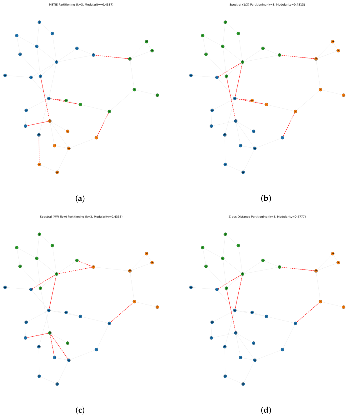
Figure 3.
Partition allocation maps for the Texas 7k synthetic grid, : (a) METIS; (b) Spectral ; (c) Z-bus distance.
Figure 3.
Partition allocation maps for the Texas 7k synthetic grid, : (a) METIS; (b) Spectral ; (c) Z-bus distance.
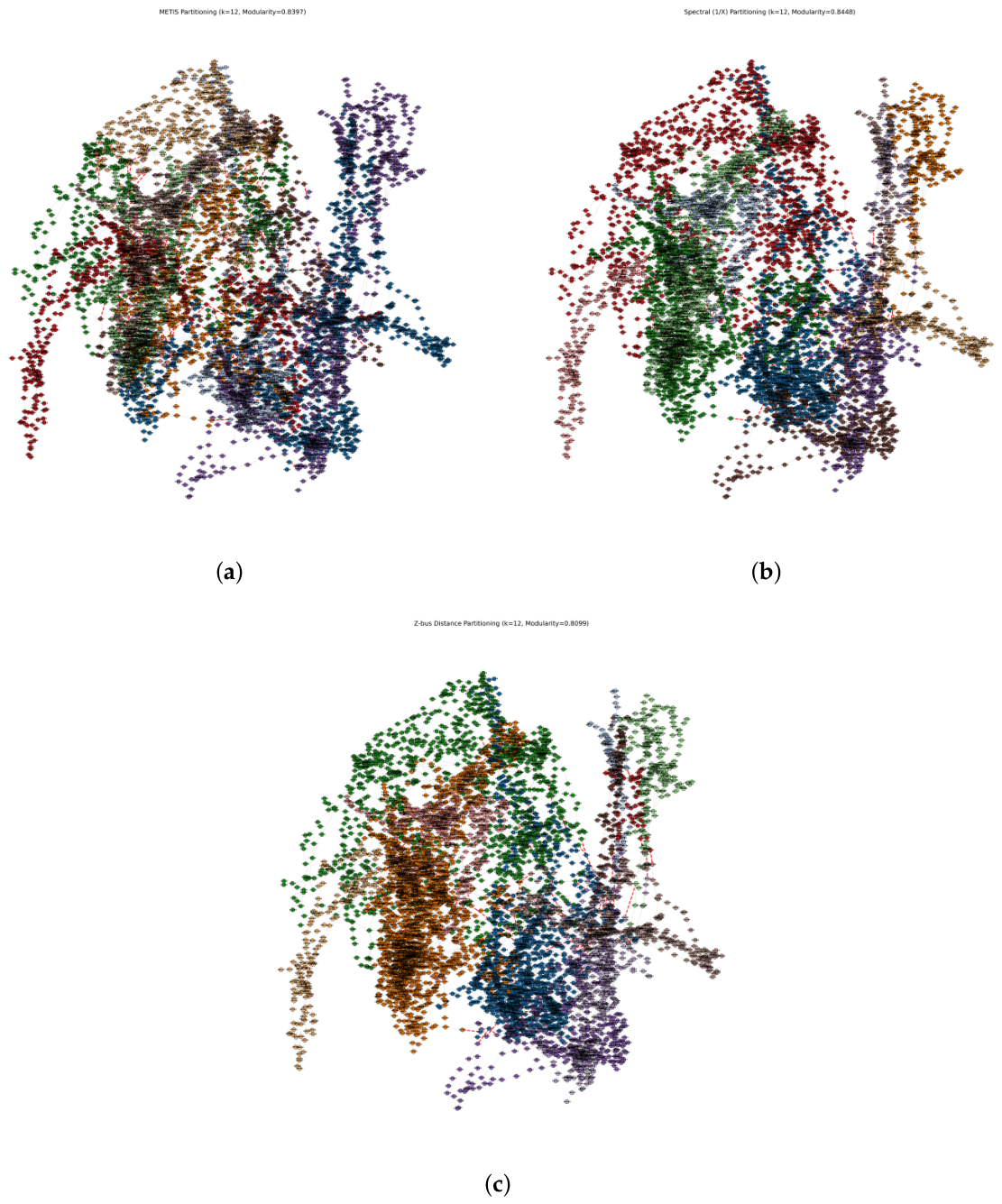
Figure 4.
Automated case splitting pipeline.
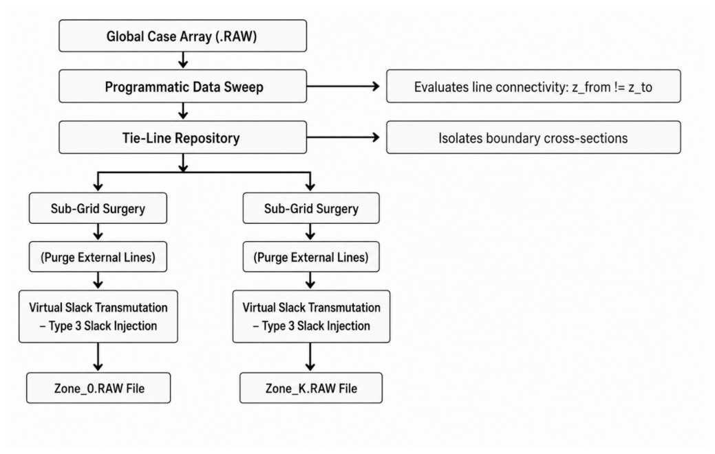
Figure 5.
PSS®E splitter output showing generated regional zones after decomposition.
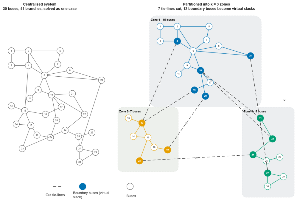
Figure 6.
Master–worker coordination loop.
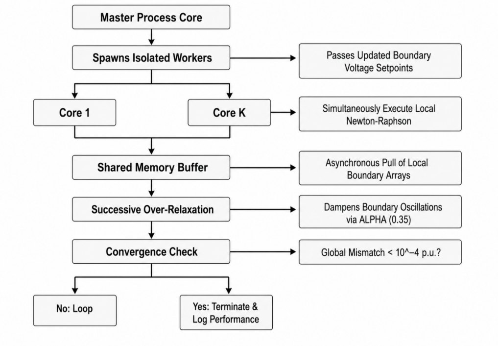

Table 1.
Test systems used for validation. Network statistics are counted directly from the PSS®E v33 RAW case files used in this study.
Table 1.
Test systems used for validation. Network statistics are counted directly from the PSS®E v33 RAW case files used in this study.
| System | Buses | Branches 1 | Generators 2 | Loads | Transformers | kV levels 3 | Base MVA | k |
|---|---|---|---|---|---|---|---|---|
| IEEE 30 bus | 30 | 41 | 6 | 21 | 4 | 3 | 100 | 3 |
| IEEE 300 bus | 300 | 411 | 69 | 197 | 105 | 13 | 100 | 6 |
| Texas 7k | 6717 | 9140 | 637 | 5095 | 1967 | 9 | 100 | 12 |
1 AC lines plus two-winding transformers; the transformer column is a subset of this total. No three-winding transformers are present. 2 In-service machines. The Texas 7k case contains a further 94 out-of-service generators, excluded from the network model. 3 Distinct nominal bus base voltages, excluding a 1.0 kV placeholder base. The IEEE 300 bus case additionally contains one
two-terminal DC link.
Table 2.
Configuration of the four candidate partitioners.
| Method | Edge Weight | Principal Limitation | Clustering Engine |
|---|---|---|---|
| Spectral (MW) | (base case) | Operating point dependent (prior power flow needed) | Spectral |
| Spectral () | Approximate coupling | Spectral | |
| Z-bus distance | , | Dense pseudoinverse | Spectral |
| METIS | Unweighted topology | Ignores electrical weighting | pymetis multilevel |
Table 3.
METIS based network partitioning.
| Algorithm 1: Generate a METIS partition for parallel power flow zoning |
|---|
| Inputs: PSS®E RAW case file; number of zones k (); random seed |
| Output: bus to zone allocation map ; partition quality metric set M |
| 01: Read the PSS®E RAW case file |
| 02: Extract all bus numbers from the BUS section and store them as graph nodes V |
| 03: Extract all AC branches from the BRANCH section and store them as graph edges E |
| 04: Extract transformer connections from the TRANSFORMER section |
| 05: For a two winding transformer, add one edge between its terminal buses |
| 06: For a three winding transformer, represent all three winding terminals in the graph using a topology preserving equivalent representation |
| 07: Construct an undirected graph , where buses are nodes and branches/transformers are edges |
| 08: Remove self loops and merge parallel circuits into single graph edges |
| 09: Convert G into the adjacency list format required by METIS |
| 10: Use METIS default options |
| 11: Apply METIS k-way partitioning to divide G into k zones |
| 12: Convert the METIS label vector into a bus to zone mapping |
| 13: For each zone, check whether the assigned buses form a connected subgraph |
| 14: If a zone is disconnected: keep the largest connected component in its original zone and reassign each smaller disconnected fragment to the neighbouring zone with the highest number of connecting edges |
| 15: End if |
| 16: Repeat the connectivity check until every zone forms a connected sub network |
| 17: Compute the quality metrics M: (1) zone sizes; (2) tie lines; (3) boundary buses; (4) modularity; (5) normalised cut; (6) connected components |
| 18: Export the final bus to zone allocation file and partition map |
Table 4.
Four method partition comparison across the three test systems.
| Method | Largest % | Size CoV | Tie-Lines | Modularity ↑ | NCut ↓ | Runtime |
|---|---|---|---|---|---|---|
| IEEE 30-bus—30 buses, 41 branches, | ||||||
| Spectral (MW) | 46.7 | 0.327 | 8 | 0.436 | 0.593 | 34.2 ms |
| Spectral () | 43.3 | 0.216 | 7 | 0.481 | 0.519 | 35.9 ms |
| Z-bus distance | 53.3 | 0.455 | 5 | 0.478 | 0.405 | 50.7 ms |
| METIS | 50.0 | 0.356 | 7 | 0.434 | 0.559 | 2.8 ms |
| IEEE 300-bus—300 buses, 411 branches, | ||||||
| Spectral (MW) | 59.3 | 1.171 | 15 | 0.571 | 0.477 | 73.3 ms |
| Spectral () | 29.0 | 0.510 | 22 | 0.732 | 0.344 | 90.8 ms |
| Z-bus distance | 34.0 | 0.604 | 25 | 0.703 | 0.339 | 116.9 ms |
| METIS | 27.0 | 0.466 | 18 | 0.739 | 0.292 | 24.7 ms |
| Texas 7k—6717 buses, 9140 branches, | ||||||
| Spectral (MW) | 28.3 | 0.982 | 234 | 0.804 | 0.395 | 31.1 s |
| Spectral () | 20.0 | 0.734 | 215 | 0.845 | 0.356 | 28.5 s |
| Z-bus distance | 28.0 | 0.991 | 171 | 0.810 | 0.354 | 312 s |
| METIS | 17.1 | 0.493 | 579 | 0.840 | 0.796 | 3.2 s |
Table 5.
Example bus to zone allocation output used as the input to the case splitter (IEEE 30bus, ).
Table 5.
Example bus to zone allocation output used as the input to the case splitter (IEEE 30bus, ).
| Bus ID | METIS | Spectral () | Spectral (MW) | Z-Bus Distance |
|---|---|---|---|---|
| 1 | 0 | 2 | 2 | 2 |
| 2 | 0 | 2 | 2 | 2 |
| 3 | 0 | 2 | 2 | 2 |
| 4 | 0 | 2 | 2 | 2 |
| 5 | 0 | 2 | 2 | 2 |
| 6 | 0 | 2 | 2 | 2 |
| 7 | 0 | 2 | 2 | 2 |
| 8 | 0 | 2 | 2 | 2 |
| 9 | 0 | 0 | 0 | 0 |
| 10 | 0 | 0 | 0 | 0 |
| 11 | 0 | 0 | 0 | 0 |
| 12 | 1 | 0 | 2 | 0 |
| 13 | 1 | 0 | 2 | 0 |
| 14 | 1 | 0 | 0 | 0 |
| 15 | 1 | 0 | 0 | 0 |
| 16 | 0 | 0 | 0 | 0 |
| 17 | 0 | 0 | 0 | 0 |
| 18 | 1 | 0 | 0 | 0 |
| 19 | 1 | 0 | 0 | 0 |
| 20 | 0 | 0 | 0 | 0 |
| 21 | 2 | 1 | 0 | 0 |
| 22 | 2 | 1 | 0 | 0 |
| 23 | 1 | 0 | 0 | 0 |
| 24 | 2 | 1 | 0 | 0 |
| 25 | 2 | 1 | 1 | 1 |
| 26 | 2 | 1 | 1 | 1 |
| 27 | 2 | 1 | 1 | 1 |
| 28 | 0 | 2 | 1 | 2 |
| 29 | 2 | 1 | 1 | 1 |
| 30 | 2 | 1 | 1 | 1 |
Table 6.
Convergence iteration counts.
| Test System | Buses (n) | Centralised NR Iterations | Outer Consensus Iterations | Workers (k) |
|---|---|---|---|---|
| IEEE 30 bus | 30 | 3 | 16 | 3 |
| IEEE 300 bus | 300 | 6 | 17 | 6 |
| Texas 7k | 6717 | 210 | 17 | 12 |
Table 7.
Wall clock time and CPU utilisation.
| Test System | Centralised NR Wall Time (s) | Distributed Wall Time (s) | Distributed Total CPU Time (s) | METIS Offline Partitioning (ms) |
|---|---|---|---|---|
| IEEE 30 bus | 0.037 | 2.165 | 2.906 | 2.8 |
| IEEE 300 bus | 0.038 | 3.022 | 5.078 | 24.7 |
| Texas 7k | 1.521 | 4.665 | 11.844 | 3169.4 |
Table 8.
Bus voltage accuracy validation.
| System | Buses Compared | Max Diff (p.u.) | Mean Diff (p.u.) | Buses > 0.01 p.u. |
|---|---|---|---|---|
| IEEE 30 bus | 30 | 0.00005 | 0.000024 | 0 |
| IEEE 300 bus | 300 | 0.00293 | 0.000372 | 0 |
| Texas 7k | 6717 | 0.03882 | 0.000418 | 11 |
Disclaimer/Publisher’s Note: The statements, opinions and data contained in all publications are solely those of the individual author(s) and contributor(s) and not of MDPI and/or the editor(s). MDPI and/or the editor(s) disclaim responsibility for any injury to people or property resulting from any ideas, methods, instructions or products referred to in the content. |
© 2026 by the authors. Licensee MDPI, Basel, Switzerland. This article is an open access article distributed under the terms and conditions of the Creative Commons Attribution (CC BY) license.
Copyright: This open access article is published under a Creative Commons CC BY 4.0 license, which permit the free download, distribution, and reuse, provided that the author and preprint are cited in any reuse.