
Submitted:
01 September 2026
Posted:
02 September 2026
You are already at the latest version
Abstract
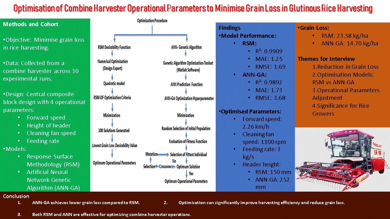
Rear-discharge grain loss during rice harvesting is governed by interacting combine-harvester settings, yet studies often rely on fitted accuracy without uncertainty-aware validation. It was hypothesized that (H1) grain loss would exhibit significant nonlinear, quadratic, and interaction effects and (H2) validation would identify a stable operating region. A four-factor, five-level central composite block design comprising 30 runs evaluated the effect of forward speed, header-height set point, cleaning-fan speed, and feed-rate set point on grain loss. Response surface methodology - desirability function (RSM-DF) and artificial neural network - genetic algorithm (ANN-GA) yielded fitted minima of 23.58 and 14.70 kg/ha, respectively. Using a reconstructed 30-run analytical dataset, quadratic RSM, regularized quadratic regression, support vector regression (SVR), Gaussian process regression (GPR), and a weighted ensemble were compared through 20 repetitions of nested five-fold cross-validation. Permutation importance, SHapley Additive exPlanations (SHAP), and 1,000 residual-bootstrap models supported interpretation and robust optimization. Quadratic RSM generalized best (R² = 0.8751; RMSE = 6.18 kg ha⁻¹; MAE = 4.56 kg ha⁻¹), while cleaning-fan speed, header height, and forward speed dominated prediction. A robust plateau of 2.26 km/h, 150 mm, 1100 rpm, and 4.5–5.0 kg/s yielded 23.96 kg/ha (95% model-uncertainty interval: 21.70–26.41). The results indicate that both RSM-DF and ANN-GA can be utilized to model the processes of combine harvester operation to achieve better optimization results.
Keywords:
grain-loss minimization
; combine harvester
; response surface methodology
; nested cross-validation
; explainable machine learning
; robust optimization
1. Introduction
Harvesting operation in rice production requires careful handling of a combine harvester to reduce grain loss. Grain loss is a critical indicator of harvesting performance and can directly reduce recoverable yield and farm income [1]. Under Malaysian paddy-field conditions, combine harvester’s field speed was positively associated with grain loss [2]. Reliable grain loss measurement is therefore essential for evaluating and improving harvesting performance. [3] reviewed sensing technologies used to measure paddy harvesting losses, while [4] developed an array-structured sensor to improve grain loss monitoring resolution during rice harvesting. Total grain loss has been recommended not to exceed 3% of the crop yield as cited in [5]. In the Malaysian paddy harvesting, [6] recorded the maximum grain loss of 1.39% and estimated income losses of up to USD 29.26/ha. In southeastern Turkey, rice harvesting losses were estimated to reach 25–30% when unsuitable machinery and techniques were used [7].
Identifying appropriate operational and field parameters are important for predicting and minimizing grain loss during harvest [8]. For maize harvesting, grain loss is influenced by forward speed, feeding amount, cylinder or rotor speed, cylinder–concave clearance, and header configuration [1]. Other cereal combine studies have shown that a drum speed could affect processing loss [9]. [10] found that reel index, cutting height, and vertical reel-to-cutter-bar distance significantly affected header loss, whereas the linear effect of horizontal reel distance was not statistically significant. [11] applied radial-basis-function and adaptive neuro-fuzzy models together with response surface methodology (RSM) to predict and optimize combine harvester’s performance. Collectively, these findings indicate that grain loss reduction requires coordinated adjustment of several interacting operational variables.
Improperly adjusted combine harvesters can generate substantial grain loss [7]. [12] found that cutter-bar working width, grain yield, forward speed, and field conditions influenced combine harvester performance. [13] reported that improper machine settings, high travel speed, and poor combine harvester condition contribute to grain loss during paddy harvesting in Malaysia. [14] identified forward speed as a main factor influencing grain loss and grain damage during harvest. Furthermore, [2] recorded operating speeds of 3.87–6.11 km/h, with the lowest observed speed associated with the lowest grain loss. Although an increased speed may improve field capacity, it can shorten the time available for cutting, threshing, separation, and cleaning. Consequently, the optimum harvest operation must balance between throughput and grain loss risk, and modelling is required to evaluate the combined effects of the relevant settings.
Response surface methodology integrates designed experimentation, polynomial model development, effect assessment, and process optimization [15,16]. Rather than assuming that a response is globally linear, RSM approximates the response locally using a low-order polynomial, thereby enabling interpretation of linear, quadratic, and interaction effects. RSM has been applied to agricultural machinery and food process optimization, including combine harvester’s cleaning fan design [17], self-propelled crop sprayer operation [18], and convective/infrared drying [19]. Artificial neural networks (ANN) provide a data-driven approach for modelling nonlinear relationships. [20] compared ANN and RSM for medium optimization of Tetraselmis sp. FTC209, while [21] compared the two methods for FAME extraction from fish waste. [22] developed an ANN to predict crushing, impurity, and grain loss rate in a flexible rice threshing device. [23] compared RSM and ANN–GA for soybean meal fermentation. In an agricultural machinery, [24] combined RSM and ANN to model and optimize the specific energy consumption and harvesting loss rate of a green forage maize harvester header. [25] similarly compared RSM and ANN in a melanin production process and reported lower prediction errors and a higher optimized response using ANN in that specific application.
Despite an increasing application of RSM and ANN-based optimizations, rigorous assessment of comparative generalization remains limited for medium-sized combine harvester for rice harvesting. Using the same resampling information for model tuning and final performance assessment can produce optimistically biased error estimates, whereas nested cross-validation reduces this model-selection bias [26]. Moreover, the uncertainty surrounding recommended operating settings and the stability of variable importance conclusions are rarely evaluated in this application area. Consequently, the comparative generalization of RSM and alternative nonlinear learners, together with the robustness and interpretability of their recommended settings, remains insufficiently established for medium-sized rice combines.
Accordingly, two hypotheses were formulated: H1, grain loss is governed by significant nonlinear, quadratic, and interaction effects among the combine harvester operating parameters; and H2, leakage-controlled validation, explainable modelling, and bootstrap optimization can identify a stable and practically interpretable operating region that is more defensible than a single fitted optimum. This study therefore aimed to: (i) quantify the effects of forward speed, header-height set point, cleaning-fan speed, and feed-rate set point using a 30-run central composite block design; (ii) compare the fitted predictions and optima obtained using RSM-DF and ANN-GA; (iii) benchmark quadratic RSM, regularized quadratic regression, support vector regression, Gaussian process regression, and a weighted ensemble through repeated nested cross-validation; (iv) interpret the validated decision model using permutation importance and SHapley Additive exPlanations (SHAP); and (v) derive an uncertainty-aware robust operating window using residual bootstrapping. The study contributes a leakage-controlled and explainable framework for more reliable combine-harvester adjustment within the investigated operational domain.
2. Materials and Methods
2.1. Study Area
The study was conducted in a one-hectare glutinous-rice field in Ayer Hangat, Langkawi Island, Malaysia (06°25′14.7″ N, 99°48′23.0″ E). The study was carried out during harvest season in 2023. Weather conditions during the experiment included an ambient air temperature of 33 °C, relative humidity of 83%, wind speed of 5 km/h, and atmospheric pressure of 1008 hPa. Pre-harvest assessments were conducted to determine crop yield, grain moisture content, and crop height. The rice variety was Pulut Siding MR4, a local glutinous-rice variety that matured approximately 116 days after germination and had an average crop height of 0.85 m, grain moisture content of 19.50%, and yield of 5870 kg/ha.
2.2. Selection of the Combine Harvester
A medium-sized tracked combine harvester manufactured by FM World Star, China, was used in this study (Figure 1). The machine had a cutting width of 2.36 m and a rated engine output of 108 hp at 2600 rpm. Before the field experiment, the combine harvester was inspected to ensure satisfactory operating conditions, and no mechanical malfunction was observed during the experimental runs. The principal technical specifications are presented in Table 1.
2.3. Grain Loss Experimental Measurement
Various equipment and instruments were used during the harvesting experiment to ensure accurate data collection. These included a measuring tape to determine plot size and the length of the machine’s swath, a stopwatch to record the harvesting time, a weighing scale to measure the weight of grains and residues, and a digital moisture meter to measure the moisture content of the grain. Additionally, a tachometer was used to measure the speed of the cleaning fan, whereas plastic containers and woven sacks were used to collect the grain samples and harvest debris. For each experimental run, the four operating factors were established according to the prescribed experimental design set points. Forward speed was controlled using the machine speed lever and determined from the time required to traverse the 30 m experimental swath. Header height was adjusted using the machine header control to the prescribed design set point. Cleaning fan speed was established using the cleaning fan level gauge and verified using a tachometer. The feed-rate set point was established using the machine feed rate monitoring control. Header height and feed rate were therefore treated as prescribed operational set points, rather than as independently measured variables. All settings were established before commencing each experimental swath.
Forward speed was calculated from the measured swath-traversal time as shown in Equation (1):
where v is the forward speed (km/h), 30 is the experimental swath length (m), t is the recorded swath-traversal time (s), and 3.6 is the conversion factor from m/s to km/h.
In this study, grain loss was operationally defined as rear-discharge grain loss, representing the recoverable grain contained in the material discharged from the rear of the combine harvester; losses occurring at the header were not included in the measured response. Rear-discharge grain loss was measured by placing a collection sack behind the combine harvester at the start of each swath to capture discharged grain, threshed heads, and crop residues (Figure 2a). The procedure was repeated for all 30 experimental runs using the operational settings prescribed by the experimental design (Figure 2b). At the end of each 30 m swath, the machine was stopped and the collection sack was removed (Figure 2c). The harvested width was 2.36 m, corresponding to the header cutting width. Each collected sample was manually screened to separate grain from non-grain material (Figure 2d–f), following conventional grain-loss measurement practice [3]. The recovered grain mass was recorded as the measured grain loss.
The grain loss recorded per unit area of harvest was determined using the relationship given in Equation (2):
where GLarea is grain loss per unit harvested area (kg/ha), GL is the mass of recovered grain collected behind the combine harvester (kg), and Ah is the harvested area represented by the collection swath (ha). For each experimental run, the harvested area represented by the collection swath was calculated from the 30 m swath length and the 2.36 m header width, as clarified in Equation (3). The recovered grain mass was divided by this harvested area to express rear-discharge grain loss in kg/ha.
2.4. Experimental Design
The experiment was conducted using RSM in a four-factor, five-level randomised central composite block design comprising 30 experimental runs. The numerical factors were combine-harvester forward speed (X1), header height set point (X2), cleaning fan speed (X3), and feed rate set point (X4), while the response was rear-discharge grain loss. A central composite design was selected because its factorial, centre, and axial points permit estimation of linear, interaction, and quadratic effects across an expanded experimental region [15,16]. Table 2 presents the coded and uncoded levels of the four operational factors. Their ranges were determined from the harvesting practices and specifications of the combine harvester investigated.
The value of 6 kg/s reported in Table 1 represents the nominal rated feeding capacity of the combine harvester. In the central composite design, the feed rate factor included a +2 axial set point of 7.5 kg/s to extend the experimental domain and permit estimation of quadratic curvature. This axial value should therefore be interpreted as an experimental-design set point rather than the manufacturer’s rated continuous feeding capacity. For practical optimisation, the feed rate search domain was subsequently restricted to 3–6 kg/s.
2.5. Grain Loss Prediction Modelling Using RSM
A second-order polynomial RSM model was fitted to the experimental data using Design-Expert software. The fitted model expressed predicted rear-discharge grain loss as a function of the independent operational variables, presented in Equation (4):
where is the predicted grain loss; is the intercept; , , and are the linear, quadratic, and interaction coefficients, respectively; and are the independent variables; k is the number of factors [16].
Analysis of variance, multiple regression, and response-surface modelling were performed using Design-Expert software, version 13.1.5 (Stat-Ease Inc., Minneapolis, MN, USA). The quadratic model comprised four linear terms, six two-factor interaction terms, and four squared terms. The statistical significance of the overall model and its individual terms was assessed using F-tests, with p<0.05 considered statistically significant. Exact p-values were reported to indicate the strength of evidence for each model term. Model adequacy was evaluated using the lack-of-fit test, coefficient of determination (R²), adjusted R², predicted R², adequate precision, residual standard deviation, and coefficient of variation. The fitted regression coefficients were subsequently used to generate the response-surface and contour plots.
2.6. Grain Loss Prediction Modelling Using ANN
A feed-forward back-propagation ANN based on a multilayer perceptron architecture was developed to model the relationship between the combine harvester operating parameters and grain loss. The network employed a 4–10–1 topology comprising four input neurons, a single hidden layer containing ten neurons, and one output neuron, as illustrated in Figure 3. The input neurons represented forward speed (km/h), header-height set point (mm), cleaning-fan speed (rpm), and feed-rate set point (kg/s), whereas the output neuron represented rear-discharge grain loss (kg/ha). Each neuron in the hidden layer was connected to all four input neurons, and the hidden-layer outputs were fully connected to the output neuron. During training, the network weights and biases were iteratively adjusted through backpropagation to minimise the prediction error.
The ANN was implemented in MATLAB R2023a. A total of 30 experimental observations were partitioned into 22 training observations, four validation observations, and four testing observations, corresponding to 73.3%, 13.3%, and 13.3% of the dataset, respectively. The training subset was used to estimate the network weights and biases, the validation subset was used to monitor generalisation and apply early stopping, and the testing subset was used to assess the trained network. Network parameters were updated through backpropagation to minimise the mean squared error between the measured and ANN-predicted grain-loss values. The network state corresponding to the minimum validation error was retained for performance evaluation.
The training objective was defined using the mean squared error cost function presented in Equation (5).
where n is the number of training observations, is the measured grain loss, is the ANN-predicted grain loss, and w and b denote the network weights and biases, respectively. During training, the weights and biases were updated iteratively to minimize C(w, b), while validation performance was monitored to apply early stopping.
2.7. Analysis of the Grain Loss Prediction Models
The predictive performances of RSM and ANN models were evaluated using the Pearson correlation coefficient (R), coefficient of determination (R²), mean absolute error (MAE), and root mean square error (RMSE), as defined in Equations (6)–(8). The Pearson correlation coefficient quantified the strength of the linear association between the measured and predicted responses, whereas R² was calculated using R²=1−SSE/SST. The same R², MAE, and RMSE definitions were applied to the supplementary machine-learning models using their out-of-fold predictions. Range-normalized RMSE and prediction bias were additionally calculated for the repeated nested-cross-validation analysis.
where n is the number of observations, is the measured grain loss, is the predicted grain loss, and is the mean measured grain loss.
2.8. Optimisation of the Combine Harvester Operational Parameters
Two approaches were used to optimise the combine harvester operating parameters: RSM with a desirability function (RSM-DF) and ANN a genetic algorithm (ANN-GA). RSM-DF optimisation was conducted in Design-Expert, whereas ANN-GA optimisation was performed in MATLAB R2023a (MathWorks, Natick, MA, USA) using the genetic-algorithm toolbox. The GA searched the bounded operating-variable space through iterative selection, crossover, mutation, and elitism. For both optimisation approaches, the response objective was to minimise predicted rear-discharge grain loss within the specified operational ranges.
2.8.1. RSM–DF Optimisation
The fitted quadratic model was used to optimise the combine harvester operating parameters. For consistency with the experimentally defined factor levels, the optimisation bounds are presented in actual operational units; cleaning fan setting levels 2-4 corresponded to rotational speeds of 1100–1500 rpm. The factors were constrained to the ranges specified in Table 3, and the response goal was set to minimise predicted grain loss. Design-Expert generated 100 candidate solutions with different combinations of the input variables. The solution with the highest overall desirability, while satisfying the factor constraints and minimising the response, was selected as the RSM-DF optimum.
2.8.2. ANN-GA Optimisation
The trained ANN was coupled with a genetic algorithm to search the bounded operating-input space, following the surrogate-model optimization structure applied by [27]. Each individual in the GA population represented a candidate operating vector comprising forward speed, header-height set point, cleaning-fan speed, and feed-rate set point. For every candidate vector, the trained ANN predicted grain loss, and this predicted response was used as the objective value to be minimized.
An initial population of candidate operating vectors was generated within the specified lower and upper bounds. Parent solutions were selected using roulette-wheel selection, while scattered crossover combined the operating-variable values of selected parents to produce new candidate solutions. Mutation was applied to maintain population diversity and reduce premature convergence, and the highest-performing feasible solutions were retained through elitism. The search continued until either the maximum number of generations or the stall-generation stopping criterion was reached. The feasible operating vector producing the lowest ANN-predicted grain loss was retained as the ANN–GA optimum. The selection, crossover, mutation, elitism, stopping criteria, and numerical GA settings were implementation choices of the present study.
The GA configuration and operational search bounds are summarized in Table 4. Population size, crossover fraction, mutation probability, maximum-generation limit, stall-generation limit, and lower and upper decision-variable bounds governed the evolutionary search.
2.8.3. Experimental Confirmation of the Optimised Operating Conditions
Following optimisation, the operating conditions selected by RSM-DF and ANN-GA approaches were evaluated experimentally in the field. For each selected condition, the forward speed, header height set point, cleaning fan speed, and feed rate set point were adjusted to the corresponding model-derived values. Grain loss was then measured using the collection and separation procedure described in Section 2.3. Grain and threshing residues discharged from the rear of the combine harvester over the 30 m swath were collected, manually separated, weighed, and converted to grain loss per harvested area in kg/ha. The experimentally measured grain loss value was compared with the corresponding model prediction, and the residual was calculated as the difference between the experimental and predicted responses. One independent field-confirmation run was conducted at each model-derived operating condition (n=1 per optimisation method).
2.9. Small-Sample Machine-Learning Benchmarking and Uncertainty-Aware Validation
A supplementary small sample machine learning benchmark was conducted to evaluate predictive performance beyond the fitted data comparison between RSM and ANN. The supplementary analysis used a reconstructed 30-run analytical dataset. Experimental grain loss and fitted prediction series were extracted from the editable Figure 10 chart data, while the row wise operating factor combinations were reconstructed from the reported central composite design structure, Table 2, and the fitted RSM model. The four operational variables expressed in actual units were used as model inputs, whereas the experimental block was excluded as a predictor. For the grouped sensitivity analysis, observations sharing an identical combination of the four coded factors were assigned to the same group so that the six centre point observations were withheld together. The same reconstructed factor response structure was applied consistently throughout the validation, explainability, and robust-optimisation analyses.
Five candidate approaches were evaluated: the unregularized quadratic RSM reference model, regularised quadratic regression, radial-basis-function support vector regression (SVR), Gaussian process regression (GPR), and a weighted ensemble of the four component models. The RSM and regularised models included the four linear terms, four squared terms, and six pairwise interactions. Ridge regularisation was applied to the expanded quadratic feature space to mitigate multicollinearity-related coefficient instability [28]. SVR was included as a kernel-based nonlinear regression learner grounded in the support-vector framework [29,30], whereas GPR was included as a probabilistic kernel-based regression approach that provides predictive distributions [31]. The ensemble prediction was calculated from inverse-inner-validation-RMSE weights, ensuring that the weighting coefficients were determined exclusively from training data. The candidate configurations and hyperparameter search spaces are presented in Table 5.
Predictive performance was estimated using repeated nested cross-validation to minimize selection bias during model tuning [26]. The outer procedure comprised five-fold cross-validation repeated 20 times, yielding 100 outer test folds and 20 complete out-of-fold prediction vectors. Within every outer training partition, four-fold inner cross-validation was used to select regularization, kernel, and error-insensitivity parameters. Identical outer partitions were applied to all models, and polynomial transformation, standardization, hyperparameter selection, and ensemble weighting were performed within the training partitions only. A base random seed of 20260804 was used to generate the outer and inner cross-validation partitions, thereby ensuring reproducible data splitting across the candidate models. Performance was quantified using the coefficient of determination (R²), RMSE, MAE, range-normalized RMSE, and prediction bias. Means, standard deviations, and bootstrap 95% confidence intervals were calculated across the 20 complete repetitions. Exploratory one-sided Wilcoxon signed-rank comparisons, followed by Holm adjustment, were applied to the paired repeat-level RMSE values. Because repeated cross-validation estimates share observations and are therefore correlated, these adjusted p-values were interpreted as descriptive consistency evidence rather than independent confirmatory tests.
A stricter leave-one-design-condition-out sensitivity analysis was additionally performed. In this analysis, all observations sharing an identical combination of the four coded factors were assigned to the same group; consequently, the six centre-point replicates were withheld together. This grouped procedure evaluated the ability of each model to predict an entirely unobserved operating combination, rather than a new replicate located within the represented design structure. The analyses were implemented in Python 3.13 using scikit-learn 1.8.0.
2.10. Explainable Artificial Intelligence and Robustness-Based Operational Analysis
The model providing the strongest repeated nested-cross-validation performance was subsequently used as the primary decision model for explainable and robustness-based analysis. Model-agnostic permutation importance was calculated within each of the 100 outer test folds by randomly permuting one operational variable 100 times and measuring the resulting increase in test RMSE. Accordingly, a large positive change in RMSE indicated that the model relied strongly on that input for unseen-data prediction, whereas a zero or negative change indicated negligible stable predictive information [32]. The fold-level importance estimates were summarised using their mean, standard deviation, and bootstrap 95% confidence interval.
SHAP were calculated using the linear SHAP framework of [33] to quantify observation-specific contributions to the fitted grain loss response. The selected quadratic model was linear in an expanded 15-column design matrix comprising the intercept and 14 polynomial terms: four linear, four squared, and six pairwise interaction terms. Exact linear SHAP values were calculated for the non-intercept terms. As a study-specific aggregation procedure, each interaction-term contribution was divided equally between its two constituent operational variables. Mean absolute SHAP values were then used to summarise global importance for forward speed, header height, cleaning fan speed, and feed rate, while the interaction terms were additionally ranked separately. Bootstrap partial-dependence profiles were generated over 51 equally spaced values for each factor while averaging over the empirical distribution of the remaining variables.
Model uncertainty was quantified using a fixed design residual bootstrap procedure based on established regression resampling principles [34]. The centred residuals of the quadratic model were resampled with replacement, and 1,000 bootstrap response vectors were generated at the original central composite design points. A new quadratic coefficient vector was fitted to each bootstrap sample. The number of bootstrap replications, practical search grid, robust optimisation criterion, and operating region thresholds were implementation choices of the present study. Residual-bootstrap resampling was initialised using a fixed random seed of 20264004 to ensure reproducibility of the bootstrap model distributions and optimisation results. The practical search domain was constrained to the same ranges employed in the analysis: 1.76–2.26 km/h of forward speed, 150–350 mm of header height, 1100–1500 rpm of cleaning fan speed (rpm), and 3–6 kg/s of feed rate. A grid of 41,327 candidate operating combinations was evaluated using every bootstrap coefficient vector.
Two optimisation criteria were considered. First, the deterministic optimum was the grid point with the minimum fitted quadratic model prediction. Second, the robust optimum was the point with the lowest upper 97.5% quantile of the bootstrap model prediction distribution. To define an operating region rather than one exact setting, each grid point was assigned the probability that its predicted loss remained within 5 kg/ha of the minimum from the corresponding bootstrap model. This tolerance approximated the cross-validated MAE of the validated RSM model. A high confidence near optimal region required a probability of at least 0.90. Because a boundary constrained solution may imply that the unconstrained optimum lies outside the practical search domain, the proportions of bootstrap optima occurring at each lower and upper factor bound were also reported. SHAP computations were implemented using SHAP 0.50.0.
3. Results
3.1. Model Fitting by RSM
In this study, experimental data obtained from glutinous rice harvesting using the medium-sized combine harvester with 30 runs of operation according to a central composite block design (CCBD) were analysed using RSM. The focus of this study was to investigate the effect of the operational factors of the combine harvester on grain loss. A regression model was developed using linear and quadratic coefficients of the experimental variables. Consecutive sum of squares and descriptive statistics were used to determine the model’s capabilities. A second-order polynomial regression equation was obtained to develop the grain-loss prediction model, as shown in Equation (9).
where is the predicted rear-discharge grain loss (kg/ha), F is forward speed (km/h), H is the header height set point (mm), Lf is the cleaning-fan machine setting level, and Q is the feed rate set point (kg/s). Cleaning fan levels 1, 2, 3, 4, and 5 correspond to 900, 1100, 1300, 1500, and 1700 rpm, respectively. The displayed equation represents the continuous operational-factor component of the fitted model; the block was treated as a categorical experimental-design effect.
The significance of the quadratic grain-loss model and its individual terms was evaluated using analysis of variance (ANOVA), as presented in Table 6. The overall model was highly significant (F=100.94, p<0.0001), confirming that the fitted quadratic formulation explained a substantial proportion of the observed grain-loss variation. Forward speed (X1), header height (X2), cleaning-fan speed (X3), the X1 X2, X1 X3 , and X2X3 interactions, and the quadratic terms , , and were significant at p<0.05. In contrast, the feed-rate main effect (X4), its interaction terms, and were not statistically significant within the investigated operational range.
The coefficient of variation expresses the residual standard deviation relative to the mean response and provides an indication of experimental precision. The CV of 6.03% indicates that the residual variation was relatively small compared with the mean grain loss of 42.48 kg/ha. Adequate precision represents the model signal relative to background noise, for which values greater than 4 are generally considered desirable [35]. The adequate-precision value of 27.99 therefore indicates a strong model signal across the investigated design space.
The coefficient of determination indicated that the quadratic model explained approximately 99% of the observed variation in grain loss (R² = 0.99). The adjusted R² of 0.98 was close to the overall R² of 0.99, indicating that accounting for the number of fitted terms caused little reduction in explained variation [15]. The predicted R² of 0.93 was also close to the adjusted R², with a difference of 0.05. Furthermore, the lack of fit was not statistically significant relative to the pure error (F=5.70, p=0.0895), indicating no statistically detectable systematic model inadequacy at the 5% significance level. Collectively, these diagnostics support the suitability of the quadratic model for describing grain-loss responses and conducting optimisation within the investigated factor ranges.
3.2. Effects of Combine-Harvester Operational Factors on Grain Loss
Grain loss is an important indicator of combine harvester performance. Under Malaysian paddy-field conditions, [2] demonstrated that grain loss increased as combine-harvester field speed increased. Minimising grain loss can improve recoverable machine output and reduce the economic consequences of harvesting losses. Accordingly, determining the effects of operational parameters is important for predicting combine-harvester performance and identifying suitable operating conditions [36].
Figure 4, Figure 5 and Figure 6 present the three-dimensional response surfaces generated from the fitted RSM model. These conditional surfaces visualise pairwise factor effects while the remaining variables are held at specified values and are useful for identifying curvature and interaction [35]. The elliptical or curved contour patterns indicate pronounced interactions among the investigated combine harvester settings. Because each plot represents only a two-factor slice of the four-factor response surface, local minima shown in these figures should not be interpreted as the global operating optimum.
Figure 4 illustrates the conditional interaction between forward speed and header height. Grain loss varied nonlinearly across the surface, with the effect of forward speed depending on the selected header-height set point. The curved contour pattern indicates that neither variable should be adjusted independently. The observed pattern may reflect speed-related changes in material intake and in the time available for cutting, threshing, separation, and cleaning, consistent with reported effects of forward speed and field conditions on combine-harvester performance and grain loss [2,12]. Because this explanation is inferential and the surface represents only a two-factor slice of the complete response, it should be interpreted together with the full four-factor optimisation rather than as a stand-alone global recommendation.
Figure 5 depicts the conditional interaction between cleaning fan speed (rpm) and forward speed. Grain loss varied nonlinearly across the surface, and the effect of cleaning-fan speed depended on the selected forward speed. Fan speed, feed rate, and upper-sieve opening have been shown to jointly influence free-grain passage and material-other-than-grain content in a combine cleaning system [37]. Accordingly, RSM demonstrates the need for joint adjustment of the operating variables but does not independently define the global optimum, which was obtained from the complete four-factor model.
Figure 6 shows the conditional interaction between cleaning fan speed (rpm) and header height. The curved contour pattern indicates that the effect of cleaning-fan speed changes with header position. Higher or lower grain-loss regions therefore depend on the joint setting rather than on a single factor. Because forward speed and feed rate were fixed when this surface was generated, the apparent pairwise minimum is conditional and may differ from the optimum obtained from the complete four-factor response model.
3.3. Artificial Neural Network Prediction of Grain Loss
A total of 30 grain loss observations obtained from the harvesting experiments were used for ANN modelling. Out of these, 22 observations were assigned to the training, while four observations each were assigned to the validation and testing. The ANN produced correlation coefficients of R=0.9982, R=0.9923, and R=0.9733 for the training, validation, and testing subsets, respectively, with an overall correlation coefficient of R=0.9786 (Figure 7). The close agreement between the experimental and ANN-predicted responses across the three subsets indicates that the network effectively captured the nonlinear relationship between the combine-harvester operating parameters and grain loss. The supplementary repeated nested-cross-validation analysis presented in Section 3.6 provides an additional assessment of model performance under systematically held-out observations.
The distributions of the residual errors between the experimental and ANN-predicted grain loss values are presented in Figure 8 for the training, validation, and testing subsets. Most of the training and validation residuals were concentrated near zero, indicating close agreement between the experimental and ANN-predicted responses for these observations. The testing distribution included several larger residuals, demonstrating that prediction accuracy varied among the held-out observations. Accordingly, the error histogram was interpreted jointly with the correlation coefficient, R², MAE, RMSE, and repeated cross-validation results rather than as an independent measure of predictive performance.
Figure 9 presents the ANN performance curves across the training epochs. The minimum validation mean squared error (MSE) was 5.9061 at epoch 5; consequently, the network parameters associated with this epoch were retained for performance assessment. Although the training MSE continued to decrease during the subsequent epochs, the validation MSE did not improve further, thereby supporting selection of the epoch-5 network through validation-based early stopping.
3.4. Comparison of RSM and ANN Prediction Models
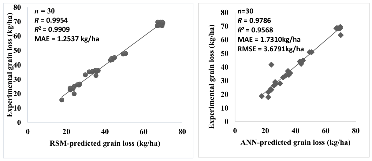
The fitted-data comparison presented in Table 7 shows that the RSM model achieved R2=0.9909, MAE = 1.2537 kg/ha, and RMSE = 1.6869 kg/ha, whereas the ANN model achieved R2=0.9568, MAE = 1.7310 kg/ha, and RMSE = 3.6791 kg/ha. The ANN predictions also exhibited a strong linear correlation with the experimental responses, with an overall Pearson correlation coefficient of R=0.9786. Accordingly, both models captured the relationship between the operating parameters and grain loss, while RSM provided a closer fitted agreement for the available experimental observations. The repeated nested-cross-validation assessment presented in Section 3.6 was subsequently used to compare the generalisation performance of the candidate models under identical held-out data partitions.
Figure 10 compares the experimental grain loss values with the corresponding fitted predictions from the RSM and ANN models. The RSM predictions were more closely distributed around the line of perfect agreement, consistent with their lower MAE and RMSE values. The ANN predictions also showed a strong positive association with the experimental observations, although several observations displayed larger residual deviations. These fitted-data plots provide a visual assessment of model agreement, while the repeated nested-cross-validation analysis in Section 3.6 evaluates prediction performance under systematically held-out observations.
Figure 10.
Relationships between the experimental grain-loss values and the fitted predictions obtained using the RSM and ANN models. The diagonal line represents perfect agreement between the experimental and predicted responses.
Figure 10.
Relationships between the experimental grain-loss values and the fitted predictions obtained using the RSM and ANN models. The diagonal line represents perfect agreement between the experimental and predicted responses.
3.5. Optimised Combine-Harvester Operating Conditions for Grain-Loss Minimisation
The fitted optima obtained using RSM-DF and ANN-GA are presented in Table 8. ANN-GA yielded a predicted minimum grain loss of 14.70 kg/ha at a forward speed of 2.26 km/h, header height of 252 mm, cleaning-fan speed of 1100 rpm, and feed rate of 3 kg/s. RSM-DF yielded a predicted minimum of 23.58 kg/ha at the same forward speed, cleaning-fan speed, and feed rate, but at a lower header height of 150 mm. Thus, the difference between the two fitted optima was associated principally with their contrasting header-height recommendations. Because each optimum was derived from its respective fitted response model, the lower ANN-GA prediction represents a model-specific optimum rather than a direct comparison of generalisation performance. Comparative predictive performance and operational robustness are evaluated in Section 3.6 and Section 3.7.
Experimental evaluation at the RSM-DF and ANN-GA operating conditions produced grain-loss values of 25.49 and 17.35 kg/ha, respectively. These values differed from the corresponding fitted predictions by 1.91 kg/ha for RSM-DF and 2.65 kg/ha for ANN-GA, indicating close local agreement for the single confirmation run conducted at each selected operating condition. Nevertheless, performance at one selected setting does not characterize prediction behaviour throughout the complete experimental domain. Therefore, the repeated cross-validation and residual-bootstrap analyses were additionally used to assess predictive performance across the investigated factor space and to derive an uncertainty-aware operating window.
3.6. Cross-Validated Predictive Performance and Uncertainty of Machine-Learning Models
The repeated nested-cross-validation results are presented in Table 9 and Figure 11. Among the five candidate approaches, the quadratic RSM model exhibited the strongest and most stable generalisation, achieving a mean R² of 0.8751 ± 0.0403, an RMSE of 6.18 ± 1.00 kg/ha, and an MAE of 4.56 ± 0.77 kg/ha. The corresponding bootstrap 95% confidence intervals were 0.8574-0.8919 for R², 5.74-6.61 kg/ha for RMSE, and 4.24-4.90 kg/ha for MAE. Thus, despite the availability of more flexible nonlinear learners, the response-surface structure remained the most appropriate representation of the small, systematically designed dataset.
Regularised quadratic regression ranked second, with a mean R² of 0.8193 and an RMSE of 7.23 kg/ha. Although shrinkage was intended to improve coefficient stability, it introduced sufficient bias to increase prediction error relative to the unregularized response-surface model. The weighted ensemble ranked third (R² = 0.8073; RMSE = 7.68 kg/ha), demonstrating that averaging the weaker kernel learners diluted rather than improved the signal captured by RSM. SVR and GPR produced lower mean R² values of 0.7404 and 0.5574 and higher RMSE values of 8.95 and 11.77 kg/ha, respectively. Exploratory paired comparisons across the 20 repetitions indicated consistently lower RSM RMSE than regularised quadratic regression (Holm-adjusted p = 0.0060), SVR (p < 0.00001), GPR (p < 0.00001), and the weighted ensemble (p = 0.000013). Given the dependence among repeated cross-validation estimates, these p-values are interpreted descriptively; the ranking, effect sizes, and uncertainty intervals provide the primary evidence that additional machine-learning complexity did not improve generalisation in this experiment.
The cross-validated RSM RMSE of 6.18 kg/ha was approximately 3.66 times its previously reported fitted-data RMSE of 1.69 kg/ha. This difference indicates that the original goodness-of-fit indices provide an optimistic estimate of performance on unseen observations, as expected when model fitting and error evaluation are based on the same limited experimental dataset. Nevertheless, the repeated-cross-validation R² remained high at 0.8751, confirming that the quadratic model retained substantial capacity to interpolate grain loss within the sampled design structure. The cross-validated estimates should therefore be considered more appropriate than the fitted-data statistics for describing anticipated prediction performance.
Under the more stringent leave-one-design-condition-out analysis, RSM remained the highest-ranked model; however, its R² declined to 0.2226, while RMSE and MAE increased to 15.61 and 9.86 kg/ha, respectively. This degradation occurred because the grouped analysis required prediction at a completely omitted operating combination, including axial boundary conditions that were not represented in the corresponding training set. Accordingly, the developed models are considerably more reliable for interpolation among combinations represented by the central composite design than for extrapolation to an unobserved operating regime. These results restrict the predictive claim to the investigated factor ranges and emphasise the need for external field validation before deployment with different machines, crop conditions, or environments.
3.7. Explainable-Model Interpretation and Robust Operating Window for Grain-Loss Minimisation
The explainability results are summarised in Table 10 and Figure 12. Cross-validated permutation importance ranked cleaning fan speed (rpm) as the most influential variable, increasing test RMSE by 9.51 kg/ha when permuted, followed closely by header height (9.28 kg/ha) and forward speed (8.65 kg/ha). Each of these variables produced a positive importance value in all 100 outer test folds. In contrast, permuting feed rate reduced RMSE by an average of 0.52 kg/ha and produced a positive change in only seven folds, indicating that feed rate supplied negligible stable predictive information within the investigated operating range.
The independent SHAP analysis yielded a consistent interpretation. Header height exhibited the largest mean absolute SHAP contribution (8.63 kg/ha), followed by cleaning-fan speed (rpm) (7.86 kg/ha) and forward speed (7.44 kg/ha), whereas the contribution of feed rate was only 0.21 kg/ha. Moreover, the forward-speed × cleaning-fan-speed interaction was the strongest interaction term, with a mean absolute contribution of 2.84 kg/ha, followed by header-height × cleaning-fan-speed at 1.45 kg/ha. This interaction structure supports the significant X1X3 and X2X3 effects identified by ANOVA and the nonlinear response patterns illustrated in Figure 5 and Figure 6. Collectively, the two explainability approaches demonstrate that adjustment of the cleaning system and header, in conjunction with forward speed, governs grain-loss variability more strongly than feed-rate adjustment.
The deterministic and robust optimisation results are presented in Table 11. Within the practical operating bounds, the refitted quadratic RSM yielded a deterministic minimum grain loss of 23.79 kg/ha at a forward speed of 2.26 km/h, header height of 150 mm, cleaning-fan speed of 1100 rpm, and feed rate of 3.00 kg/s. This result closely matched the RSM-DF prediction of 23.58 kg/ha obtained at the same operating settings, thereby demonstrating consistency between the fitted response-surface formulations. When the optimisation objective was changed from minimising the fitted mean response to minimising the upper 97.5% quantile of the bootstrap model-prediction distribution, the first three operating settings remained unchanged, while the feed rate shifted to 4.75 kg/s.
The high-confidence operating region did not support a uniquely defined feed-rate value. A probability of at least 90% of remaining within 5 kg/ha of the bootstrap-specific optimum was obtained at a forward speed of 2.26 km/h, a header height of 150–162.5 mm, a cleaning-fan speed of 1100 rpm, and feed rates of 3.0–6.0 kg/s. Nevertheless, the lowest upper model-uncertainty bound occurred at approximately 4.5–5.0 kg/s, which was selected as the centre of the preferred robust plateau (Figure 13). The broad feed-rate tolerance is consistent with its negligible permutation and SHAP importance. A secondary 80% probability region occurred at a header height of 350 mm; because it was disconnected from the principal low-header region, it was not included in the preferred operational recommendation.
At the ANN-GA operating condition of 2.26 km/h forward speed, 252 mm header height, 1100 rpm cleaning-fan speed, and 3 kg/s feed rate, ANN-GA predicted a grain loss of 14.70 kg/ha, while the corresponding experimental value was 17.35 kg/ha. At the same operating condition, the validated quadratic RSM predicted 36.51 kg/ha, with a bootstrap 95% model-uncertainty interval of 34.31–39.01 kg/ha. The difference between these predictions demonstrates that the ANN and quadratic RSM represented the header-height response differently in this region of the factor space. Accordingly, the ANN-GA setting provides a locally confirmed optimum for the ANN response model, whereas the robust RSM operating window represents the recommendation obtained from repeated cross-validation, explainability analysis, and residual-bootstrap optimisation. The two recommendations were therefore evaluated separately rather than combined into a single averaged operating condition.
The bootstrap optimum occurred at the upper forward-speed boundary in 95.1% of the models, the lower header-height boundary in 96.7%, and the lower cleaning-fan-speed boundary in 95.1%. Consequently, the recommended condition represents a boundary-constrained solution within the investigated operational domain rather than an unrestricted global optimum. The results support a preferred operating plateau of approximately 2.26 km/h forward speed, a 150 mm header-height setpoint, an 1100 rpm cleaning-fan speed, and a 4.5–5.0 kg/s feed-rate setpoint. This operating window is intended for interpolation within the investigated factor ranges; additional field evaluation across different harvesting conditions would further establish its transferability for broader operational deployment. Future implementation could also investigate coupling the validated operating recommendations with real-time sensing and data-acquisition systems to support adaptive field adjustment. In a different agricultural process, [38] demonstrated that an integrated multi-parameter sensor network combining continuous sensing, wireless data acquisition, and analytical processing can support real-time monitoring and feedback-oriented process management; analogous sensor–analytics integration may therefore provide a useful pathway for future combine-harvester decision-support systems.
5. Conclusions
Rear-discharge grain loss from the medium-sized combine harvester was governed by nonlinear and interactive effects of forward speed, header height set point, cleaning fan speed, and feed rate set point. ANN-GA yielded the lowest fitted optimum of 14.70 kg/ha and an experimental value of 17.35 kg/ha at its selected operating condition; however, within the reconstructed 30-run analytical dataset, repeated nested five-fold cross-validation identified quadratic RSM as the strongest predictive model across the investigated design space, with R² = 0.8751, RMSE = 6.18 kg/ha, and MAE = 4.56 kg/ha. Quadratic RSM ranked ahead of regularised quadratic regression, SVR, GPR, and the weighted ensemble under the common cross-validation protocol. Permutation importance and SHAP consistently showed that cleaning-fan speed (rpm), header height, and forward speed dominated prediction, whereas feed rate contributed negligible stable information. Residual-bootstrap optimisation identified a robust operating plateau of 2.26 km/h forward speed, 150 mm header height, 1100 rpm cleaning-fan speed, and 4.5–5.0 kg/s feed rate, with a mean predicted loss of 23.96 kg/ha and a bootstrap 95% model-uncertainty interval of 21.70–26.41 kg/ha. Prediction performance decreased when complete operating combinations were excluded from model development, indicating that the proposed models are most appropriate for interpolation within the investigated experimental domain. Further field evaluation under additional machines, rice varieties, field conditions, and environments would strengthen the transferability of the recommended operating window. The proposed uncertainty-aware, explainable workflow supports more defensible operator settings, reduced harvesting losses, and precision rice production.
Author Contributions
A.G.N.; Conceptualization, Methodology, Software, Formal analysis, Investigation, Data curation, Validation, Visualization, Writing – original draft, Writing – review & editing. B.M.I.; Writing – original draft, Visualization, Validation, Software, Methodology, Data curation, Conceptualisation. N.M.N.; Writing – review & editing, Visualization, Resources, Funding acquisition, Formal analysis, Data curation. S.A.A.; Writing – review & editing. M.S.M.K.; Writing – review & editing. All authors have read and agreed to the published version of the manuscript.
Funding
This research was funded by the Ministry of Higher Education of Malaysia under the Trans-disciplinary Research Grant Scheme (TRGS/1/2020/UPM/7).
Data Availability Statement
The original contributions presented in this study are included in the article. Further inquiries can be directed to the corresponding author.
Acknowledgments
The authors gratefully acknowledge the technical, logistical, and institutional support that contributed to the successful completion of this research.
Conflicts of Interest
The authors declare that they have no known competing financial interests or personal relationships that could have appeared to influence the work reported in this paper.
Abbreviations
The following abbreviations are used in this manuscript:
| RSM-DF | Response Surface Methodology - Desirability Function |
| ANN-GA | Artificial Neural Network - Genetic Algorithm |
| CCBD | Central Composite Block Design |
| FF-BP | Feed-Forward Back-Propagation |
| MLP | Multilayer Perceptron |
| SVR | Support Vector Regression |
| GPR | Gaussian Process Regression |
| SHAP | SHapley Additive exPlanations |
| CV | Cross-Validation / Coefficient of Variation |
| MAE | Mean Absolute Error |
| RMSE | Root Mean Square Error |
| R² | Coefficient of Determination |
| A.D. | Adequate Precision |
References
- Wang, K. R.; Xie, R. Z.; Ming, B.; Hou, P.; Xue, J.; Li, S. K. Review of combine harvester losses for maize and influencing factors. Int. J. Agric. Biol. Eng. 2021, 14(1), 1–10. [Google Scholar] [CrossRef]
- Mokhtor, S. A.; El Pebrian, D.; Johari, N. A. A. Actual field speed of rice combine harvester and its influence on grain loss in Malaysian paddy field. J. Saudi Soc. Agric. Sci. 2020, 19(6), 422–425. [Google Scholar] [CrossRef]
- Bomoi, M. I.; Mat Nawi, N.; Abd Aziz, S.; Mohd Kassim, M. S. Sensing technologies for measuring grain loss during harvest in paddy field: A review. AgriEngineering 2022, 4(1), 292–310. [Google Scholar] [CrossRef]
- Liang, Z.; Li, Y.; Xu, L.; Zhao, Z.; Tang, Z. Optimum design of an array structure for the grain loss sensor to upgrade its resolution for harvesting rice in a combine harvester. Biosyst. Eng. 157 2017, 24–34. [Google Scholar] [CrossRef]
- Bhardwaj, M.; Dogra, R.; Javed, M.; Singh, M.; Dogra, B. Optimization of conventional combine harvester to reduce combine losses for basmati rice (Oryza sativa). Agric. Sci. 2021, 12(3), 259–272. [Google Scholar] [CrossRef]
- Sharifuddin, M. N. Z.; Mustaffha, S. Preliminary assessment of grain losses for paddy combine harvester in Koperasi FELCRA Seberang Perak, Malaysia. IOP Conf. Ser. Earth Environ. Sci. 2021, 757(1), 012030. [Google Scholar] [CrossRef]
- Esgici, R.; Sessiz, A.; Bayhan, Y. The relationship between the age of combine harvester and grain losses for paddy. Mech. Agric. Conserv. Resour. 2016, 62(1), 18–21. [Google Scholar]
- Johari, N. A. A.; El Pebrian, D.; Mokhtor, S. A.; Mohammad, R.; Ahmad, A. H. Modelling the effect of some operational parameters on grain loss in mechanised rice harvesting: A case study in Malaysian paddy fields. Int. J. Agric. Resour. Gov. Ecol. 2020, 16(1), 23–32. [Google Scholar] [CrossRef]
- Mostofi Sarkari, M. R. Field evaluation of grain loss monitoring on combine JD 955. Adv. Environ. Biol. 2010, 4(2), 162–167. [Google Scholar]
- Zareei, S.; Abdollahpour, S. Modeling the optimal factors affecting combine harvester header losses. Agric. Eng. Int. CIGR J. 2016, 18(2), 60–65. Available online: https://cigrjournal.org/index.php/Ejounral/article/view/3701.
- Gundoshmian, T. M.; Ardabili, S.; Mosavi, A.; Várkonyi-Kóczy, A. R. Prediction of combine harvester performance using hybrid machine learning modeling and response surface methodology. In Engineering for sustainable future: Selected papers of the 18th International Conference on Global Research and Education Inter-Academia–2019 (Lecture Notes in Networks and Systems; Várkonyi-Kóczy, A. R., Ed.; Springer, 2020; Vol. 101, pp. 345–360. [Google Scholar] [CrossRef]
- Špokas, L.; Adamčuk, V.; Bulgakov, V.; Nozdrovický, L. The experimental research of combine harvesters. Res. Agric. Eng. 2016, 62(3), 106–112. [Google Scholar] [CrossRef]
- Shahar, A.; Harun, A.; Ahmad, M. T.; Ahmad, R.; Sahari, Y. (2017, February 2). In Postharvest management of rice for sustainable food security in Malaysia; FFTC Agricultural Policy Platform. https://ap.fftc.org.tw/article/1162.
- Jawalekar, S. B.; Shelare, S. D. Development and performance analysis of low-cost combined harvester for rabi crops. Agric. Eng. Int. CIGR J. 2020, 22(1), 197–201. Available online: https://cigrjournal.org/index.php/Ejounral/article/view/5429.
- Myers, R. H.; Montgomery, D. C.; Anderson-Cook, C. M. Response surface methodology: Process and product optimization using designed experiments, 4th ed.; John Wiley & Sons, 2016. [Google Scholar]
- Montgomery, D. C. Design and analysis of experiments, 9th ed.; Wiley, 2017. [Google Scholar]
- Chai, X.; Xu, L.; Sun, Y.; Liang, Z.; Lu, E.; Li, Y. Development of a cleaning fan for a rice combine harvester using computational fluid dynamics and response surface methodology to optimise outlet airflow distribution. Biosyst. Eng. 192 2020, 232–244. [Google Scholar] [CrossRef]
- Khan, F. A.; Ghafoor, A.; Khan, M. A.; Chattha, M. U.; Khorsandi Kouhanestani, F. Parameter optimization of newly developed self-propelled variable height crop sprayer using response surface methodology (RSM) approach. Agriculture 2022, 12(3), 408. [Google Scholar] [CrossRef]
- Joudi-Sarighayeh, F.; Abbaspour-Gilandeh, Y.; Kaveh, M.; Szymanek, M.; Kulig, R. Response surface methodology approach for predicting convective/infrared drying, quality, bioactive and vitamin C characteristics of pumpkin slices. Foods 2023, 12(5), 1114. [Google Scholar] [CrossRef] [PubMed]
- Mohamed, M. S.; Tan, J. S.; Mohamad, R.; Mokhtar, M. N.; Ariff, A. B. Comparative analyses of response surface methodology and artificial neural network on medium optimization for Tetraselmis sp. FTC209 grown under mixotrophic condition. Sci. World J. 2013 2013, 948940. [Google Scholar] [CrossRef] [PubMed]
- Mat Yasin, N. H.; Fakhrudin, A. S.; Abdul Hadi, A. W. A.; Mohd Khairuddin, M. H.; Abu Sepian, N. R.; Mohd Said, F.; Zainol, N. Comparison of response surface methodology and artificial neural network for the solvent extraction of fatty acid methyl ester from fish waste. Int. J. Mod. Agric. 2020, 9(3), 1929–1942. [Google Scholar]
- Ma, L.; Xie, F.; Liu, D.; Wang, X.; Zhang, Z. An application of artificial neural network for predicting threshing performance in a flexible threshing device. Agriculture 2023, 13(4), 788. [Google Scholar] [CrossRef]
- Mukherjee, R.; Chakraborty, R.; Dutta, A. Comparison of optimization approaches (response surface methodology and artificial neural network-genetic algorithm) for a novel mixed culture approach in soybean meal fermentation. J. Food Process Eng. 2019, 42(5), e13124. [Google Scholar] [CrossRef]
- Xue, Z.; Fu, J.; Fu, Q.; Li, X.; Chen, Z. Modeling and optimizing the performance of green forage maize harvester header using a combined response surface methodology–artificial neural network approach. Agriculture 2023, 13(10), 1890. [Google Scholar] [CrossRef]
- Saber, W. E. I. A.; Ghoniem, A. A.; Al-Otibi, F. O.; El-Hersh, M. S.; Eldadamony, N. M.; Menaa, F.; Elattar, K. M. A comparative study using response surface methodology and artificial neural network towards optimized production of melanin by Aureobasidium pullulans AKW. Sci. Rep. 13 2023, 13545. [Google Scholar] [CrossRef] [PubMed]
- Varma, S.; Simon, R. Bias in error estimation when using cross-validation for model selection. BMC Bioinform. 7 2006, 91. [Google Scholar] [CrossRef] [PubMed]
- Ramezanpour, M. R.; Farajpour, M. Application of artificial neural networks and genetic algorithm to predict and optimize greenhouse banana fruit yield through nitrogen, potassium and magnesium. PLoS ONE 2022, 17(2), e0264040. [Google Scholar] [CrossRef] [PubMed]
- Hoerl, A. E.; Kennard, R. W. Ridge regression: Biased estimation for nonorthogonal problems. Technometrics 1970, 12(1), 55–67. [Google Scholar] [CrossRef]
- Cortes, C.; Vapnik, V. Support-vector networks. Mach. Learn. 1995, 20(3), 273–297. [Google Scholar] [CrossRef]
- Drucker, H.; Burges, C. J. C.; Kaufman, L.; Smola, A. J.; Vapnik, V. Support vector regression machines. In Advances in neural information processing systems; Mozer, M. C., Jordan, M. I., Petsche, T., Eds.; MIT Press, 1996; Volume 9, pp. 155–161. [Google Scholar]
- Rasmussen, C. E.; Williams, C. K. I. Gaussian processes for machine learning; MIT Press, 2006. [Google Scholar] [CrossRef]
- Fisher, A.; Rudin, C.; Dominici, F. All models are wrong, but many are useful: Learning a variable’s importance by studying an entire class of prediction models simultaneously. J. Mach. Learn. Res. 2019, 20(177), 1–81. Available online: https://www.jmlr.org/papers/v20/18-760.html.
- Lundberg, S. M.; Lee, S.-I. A unified approach to interpreting model predictions. In Advances in neural information processing systems; Guyon, I., von Luxburg, U., Bengio, S., Wallach, H. M., Fergus, R., Vishwanathan, S. V. N., Garnett, R., Eds.; Curran Associates, Inc., 2017; Vol. 30, pp. 4765–4774. Available online: https://proceedings.neurips.cc/paper_files/paper/2017/hash/8a20a8621978632d76c43dfd28b67767-Abstract.html.
- Efron, B.; Tibshirani, R. J. An introduction to the bootstrap; Chapman & Hall, 1993. [Google Scholar]
- Muhammad, A. I.; Isiaka, M.; Attanda, M. L.; Shittu, S. K.; Lawan, I.; Bomoi, M. I. Performance optimization of groundnut shelling using response surface methodology. Acta Technol. Agric. 2021, 24(1), 1–7. [Google Scholar] [CrossRef]
- Bawatharani, R.; Jayatissa, D. N.; Dharmasena, D. A. N.; Bandara, M. H. M. A. Field performance of a conventional combine harvester in harvesting BG-300 paddy variety in Batticaloa, Sri Lanka. Int. J. Eng. Res. 2015, 4(1), 33–35. [Google Scholar] [CrossRef]
- Mirzazadeh, A.; Abdollahpour, S.; Hakimzadeh, M. Optimized mathematical model of a grain cleaning system functioning in a combine harvester using response surface methodology. Acta Technol. Agric. 2022, 25(1), 20–26. [Google Scholar] [CrossRef]
- Naser, A. G.; Nawi, N. M.; Zakaria, M. R.; Kassim, M. S. M.; Mutalovich, A. A.; Nasir, M. A. M. Design and implementation of an integrated sensor network for monitoring abiotic parameters during composting. Sustainability 2025, 17(21), 9780. [Google Scholar] [CrossRef]
Figure 1.
The medium-sized tracked combine harvester used in the field experiment.
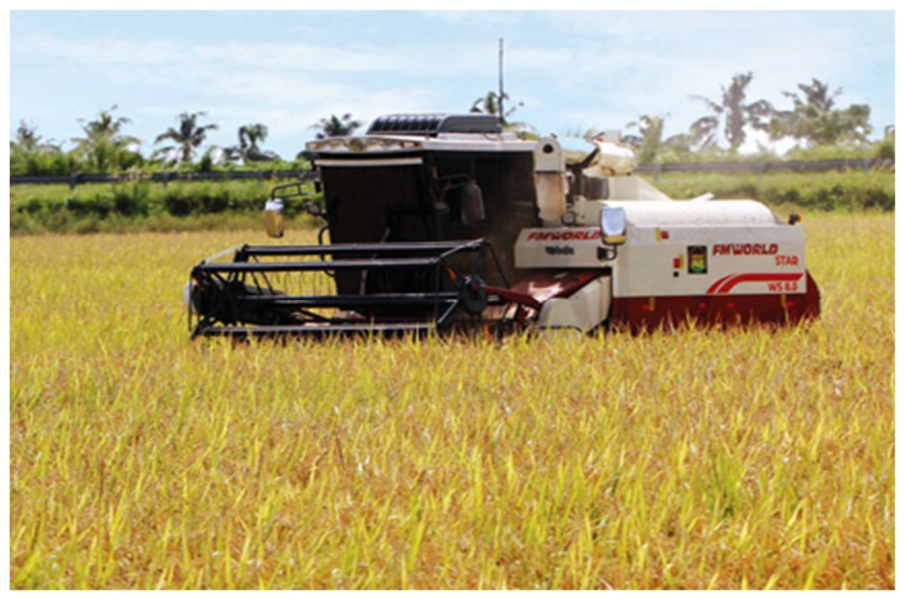
Figure 2.
Procedure for measuring grain loss; (a) placing a sack behind combine harvester, (b) combine harvester experimental run, (c) removing a sack behind combine harvester, (d) major separation of grain, (e) and (f) minor separation of grain from non-grain materials.
Figure 2.
Procedure for measuring grain loss; (a) placing a sack behind combine harvester, (b) combine harvester experimental run, (c) removing a sack behind combine harvester, (d) major separation of grain, (e) and (f) minor separation of grain from non-grain materials.
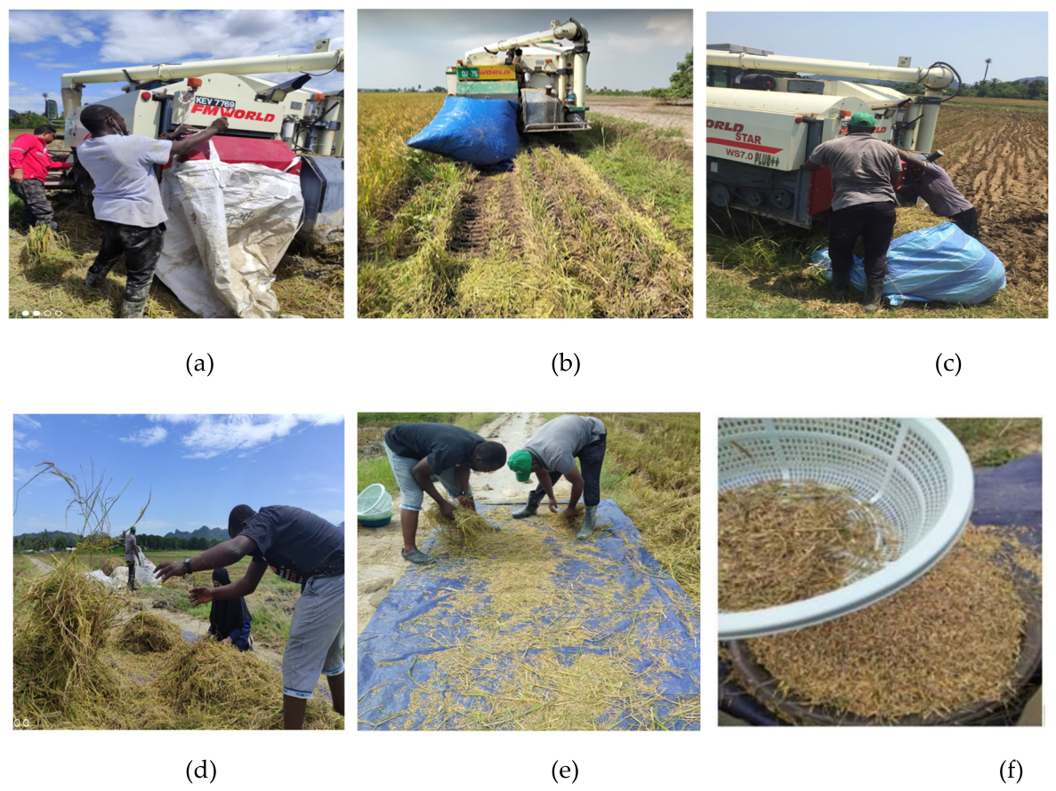
Figure 3.
Architecture of the 4–10–1 feed-forward back-propagation artificial neural network used for grain-loss prediction.
Figure 3.
Architecture of the 4–10–1 feed-forward back-propagation artificial neural network used for grain-loss prediction.
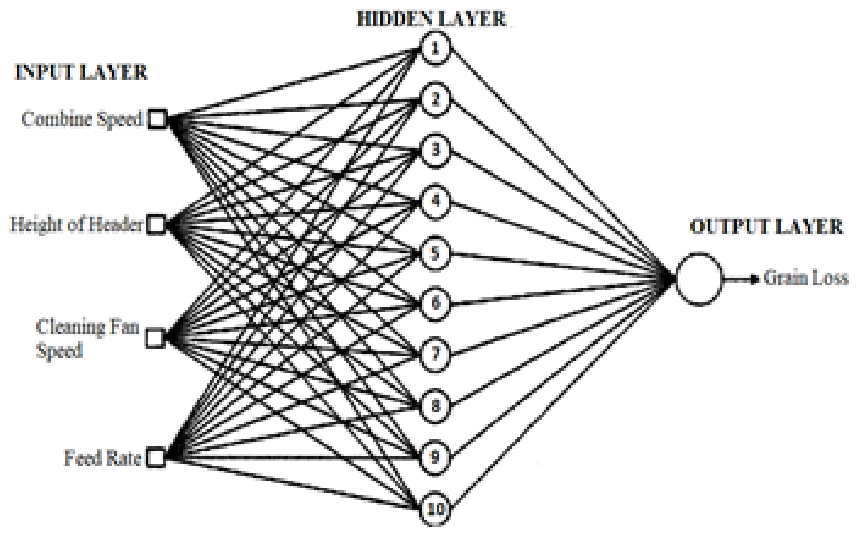
Figure 4.
Effects of combine harvester forward speed and header height set point on rear-discharge grain loss.
Figure 4.
Effects of combine harvester forward speed and header height set point on rear-discharge grain loss.
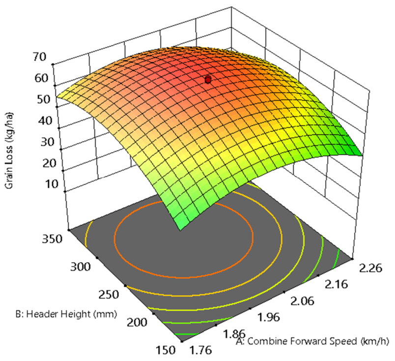
Figure 5.
Effect of cleaning-fan speed and combine-harvester forward speed on rear-discharge grain loss.
Figure 5.
Effect of cleaning-fan speed and combine-harvester forward speed on rear-discharge grain loss.
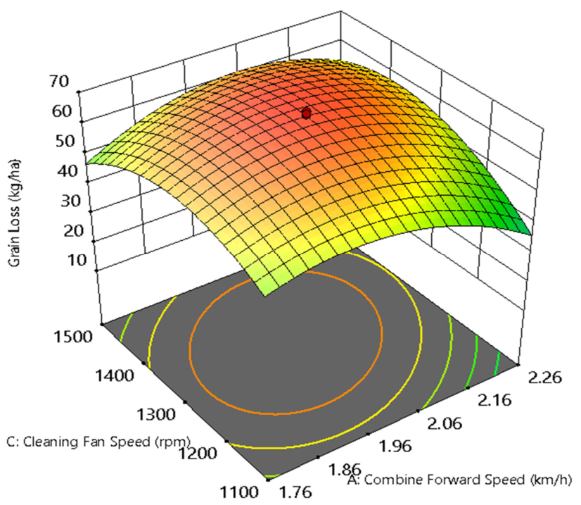
Figure 6.
Effect of header height set point and cleaning-fan speed on rear-discharge grain loss.
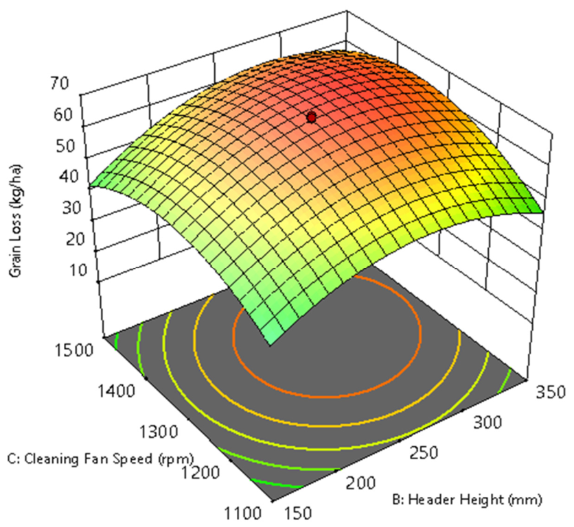
Figure 7.
Neural network training, testing and validation results for grain loss prediction.
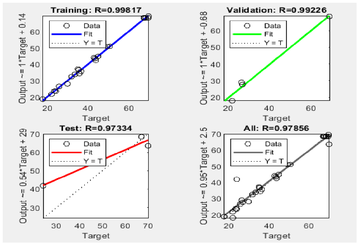
Figure 8.
Error histogram of the grain loss prediction model.
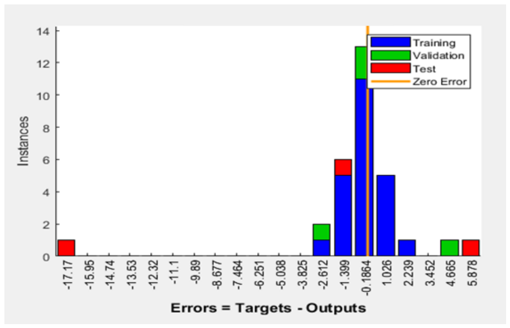
Figure 9.
Performance index for the neural network grain loss prediction model.
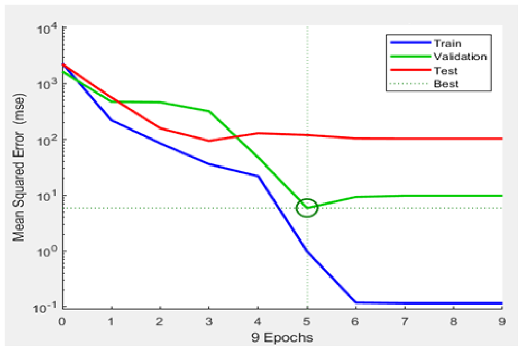
Figure 11.
Repeated nested-cross-validation RMSE of the candidate grain-loss models; error bars indicate bootstrap 95% confidence intervals for the mean across 20 complete repetitions.
Figure 11.
Repeated nested-cross-validation RMSE of the candidate grain-loss models; error bars indicate bootstrap 95% confidence intervals for the mean across 20 complete repetitions.
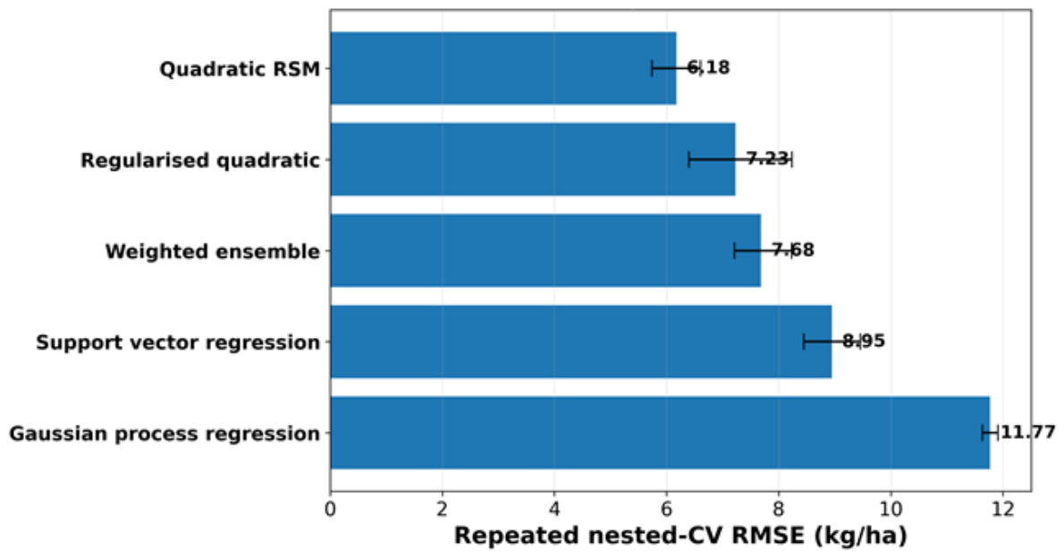
Figure 12.
Explainable assessment of operational-variable importance: (a) repeated cross-validated permutation importance and (b) global SHAP attribution of the quadratic response model.
Figure 12.
Explainable assessment of operational-variable importance: (a) repeated cross-validated permutation importance and (b) global SHAP attribution of the quadratic response model.
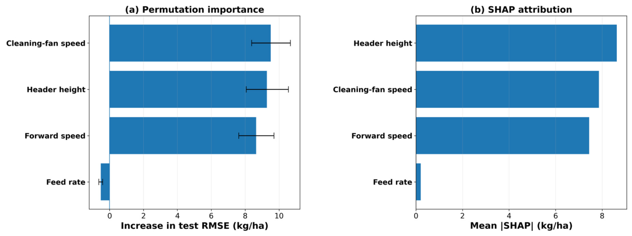
Figure 13.
Residual-bootstrap feed-rate profile at 2.26 km/h forward speed, 150 mm header height, and 1100 rpm cleaning-fan speed; the shaded vertical region denotes the preferred robust plateau.
Figure 13.
Residual-bootstrap feed-rate profile at 2.26 km/h forward speed, 150 mm header height, and 1100 rpm cleaning-fan speed; the shaded vertical region denotes the preferred robust plateau.
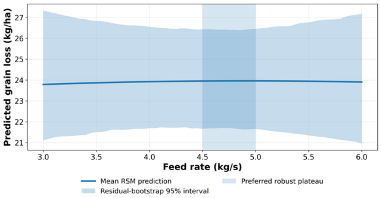

Table 1.
Principal technical specifications of the medium-sized combine harvester used in the field experiment.
Table 1.
Principal technical specifications of the medium-sized combine harvester used in the field experiment.
| Parameters | Specifications |
| Model | WS 7.0 Plus++ |
| Manufacturer | FM World Star |
| Engine model | 4G33-TC |
| Rated engine power | 80.5 kW (108 hp) |
| Rated engine speed | 2600 rpm |
| Fuel tank capacity (L) | 130 |
| Track type | Rubber track |
| Cutting width (m) | 2.36 |
| Nominal rated feeding capacity (kg/s) | 6 |
| Threshing type | Axial flow, beater bar |
| Threshing cylinder (mm) | 620 × 2010 |
| Fan type | Centrifugal fan |
| Grain-tank capacity (m³) | 1.7 |
| Unloading discharge (kg/s) | 1.68 |
Table 2.
Coded and uncoded levels of independent variables used in the central composite design.
| Factor | Unit | Symbol | −2 | −1 | 0 | +1 | +2 |
| Forward speed | km/h | (X1) | 1.51 | 1.76 | 2.01 | 2.26 | 2.51 |
| Header height | mm | (X2) | 50 | 150 | 250 | 350 | 450 |
| Cleaning fan speed | rpm | (X3) | 900 | 1100 | 1300 | 1500 | 1700 |
| Feed rate set point | kg/s | (X4) | 1.5 | 3.0 | 4.5 | 6.0 | 7.5 |
Note: The feed-rate values represent the prescribed machine operating set points used in the experimental design. The +2 axial value of 7.5 kg/s extended beyond the nominal rated feeding capacity of 6 kg/s for response-surface curvature estimation; the subsequent optimisation domain was restricted to 3–6 kg/s.
Table 3.
Response surface method optimisation criteria.
| Parameter | Goal | Lower Limit | Upper Limit | Lower Weight | Upper Weight | Importance |
| X1 | range | 1.76 | 2.26 | 1 | 1 | 3 |
| X2 | range | 150 | 350 | 1 | 1 | 3 |
| X3 | range | 1100 | 1500 | 1 | 1 | 3 |
| X4 | range | 3 | 6 | 1 | 1 | 3 |
| Grain Loss | minimise | 17.68 | 70 | 1 | 1 | 3 |
X1 : forward speed (km/h); X2 : header height set point (mm); X3 : cleaning fan speed (rpm); and X4: feed rate set point (kg/s). Cleaning fan setting levels 2, 3, and 4 corresponded to 1100, 1300, and 1500 rpm, respectively.
Table 4.
Genetic-algorithm configuration and operational search bounds.
| GA setting | Value |
| Fitness function | ANN-predicted grain loss, minimized |
| Population size | 100 |
| Mutation probability | 0.01 |
| Crossover fraction | 0.50 |
| Maximum generations | 500 |
| Stall-generation limit | 10 |
| Crossover function | Scattered crossover |
| Selection function | Roulette-wheel selection |
| Decision variables | Forward speed (km/h), header-height set point (mm), cleaning-fan speed (rpm), and feed-rate set point (kg/s) |
| Lower bounds | [1.76, 150, 1100, 3] |
| Upper bounds | [2.26, 350, 1500, 6] |
The lower- and upper-bound vectors follow the decision-variable order: forward speed, header-height set point, cleaning-fan speed, and feed-rate set point.
Table 5.
Candidate regression models and nested hyperparameter-search spaces.
| Model | Implementation | Inner-validation search space |
| Quadratic RSM | Four linear, four squared, and six pairwise interaction terms | No tunable hyperparameter |
| Regularized quadratic | Quadratic polynomial features followed by ridge regression | α = 0.01, 0.1, 1, or 10 |
| Support vector regression | Standardized radial-basis-function SVR | C = 1, 10, or 100; γ = scale, 0.1, or 1; ε = 0.1 or 1 |
| Gaussian process regression | Standardized GPR with fixed kernel candidates | RBF, Matérn ν = 1.5, or rational-quadratic kernel; noise = 0.01 or 1.0 |
| Weighted ensemble | Inverse-inner-RMSE weighting of RSM, ridge, SVR, and GPR predictions | Weights recalculated within each outer training partition |
Table 6.
Analysis of variance and model-fit statistics for the quadratic grain loss prediction model.
Table 6.
Analysis of variance and model-fit statistics for the quadratic grain loss prediction model.
| Source | Sum of Squares | df | Mean Square | F-value | p-value | |
| Block | 35 | 2 | 17.5 | |||
| Model | 9278.97 | 14 | 662.78 | 100.94 | < 0.0001 | significant |
| X1 | 116.6 | 1 | 116.6 | 17.76 | 0.001 | |
| X2 | 633.86 | 1 | 633.86 | 96.54 | < 0.0001 | |
| X3 | 259.91 | 1 | 259.91 | 39.58 | < 0.0001 | |
| X4 | 0.3851 | 1 | 0.3851 | 0.0586 | 0.8124 | |
| X1 X2 | 35.76 | 1 | 35.76 | 5.45 | 0.0363 | |
| X1 X3 | 467.64 | 1 | 467.64 | 71.22 | < 0.0001 | |
| X1 X4 | 0.297 | 1 | 0.297 | 0.0452 | 0.8349 | |
| X2 X3 | 89.4 | 1 | 89.4 | 13.62 | 0.0027 | |
| X2 X4 | 2.21 | 1 | 2.21 | 0.3359 | 0.5721 | |
| X3 X4 | 0.1089 | 1 | 0.1089 | 0.0166 | 0.8995 | |
| X1² | 2939.52 | 1 | 2939.52 | 447.69 | < 0.0001 | |
| X2² | 3278.13 | 1 | 3278.13 | 499.26 | < 0.0001 | |
| X3² | 3191 | 1 | 3191 | 485.99 | < 0.0001 | |
| X4² | 0.1064 | 1 | 0.1064 | 0.0162 | 0.9006 | |
| Residual | 85.36 | 13 | 6.57 | |||
| Lack of Fit | 81.09 | 10 | 8.11 | 5.7 | 0.0895 | not significant |
| Pure Error | 4.27 | 3 | 1.42 | |||
| Cor Total | 9399.33 | 29 | ||||
| Std. Dev. 2.56 |
R2 0.99 |
Adjusted R2 0.98 | Predicted R2 0.93 |
A.D 27.99 |
Mean 42.48 |
C.V. % 6.03 |
X1 : forward speed (km/h); X2 : header height set point (mm); X3 : cleaning fan speed (rpm); X4 : feed rate set point (kg/s); A.D.: adequate precision; C.V.: coefficient of variation; and R2: coefficient of determination.
Table 7.
Fitted-data prediction-performance comparison between the RSM and ANN models.
| Performance Parameters | Prediction Models | |
| RSM | ANN | |
| Pearson (R) | 0.9954 | 0.9786 |
| (R2) | 0.9909 | 0.9568 |
| MAE (kg/ha) | 1.2537 | 1.7310 |
| RMSE (kg/ha) | 1.6869 | 3.6791 |
Table 8.
Predicted and experimental grain loss at the optimum combine-harvester operating conditions.
Table 8.
Predicted and experimental grain loss at the optimum combine-harvester operating conditions.
| Optimum Conditions | RSM-DF | ANN-GA |
| Forward speed (km/h) | 2.26 | 2.26 |
| Header height set point (mm) | 150 | 252 |
| Cleaning-fan speed (rpm) | 1100 | 1100 |
| Feed-rate set point (kg/s) | 3 | 3 |
| Response | ||
| Predicted rear-discharge grain loss (kg/ha) | 23.58 | 14.70 |
| Experimental rear-discharge grain loss (kg/ha) | 25.49 | 17.35 |
Table 9.
Repeated nested-cross-validation performance of the candidate grain-loss models.
| Model | R², mean ± SD (95% CI) | RMSE, kg/ha, mean ± SD (95% CI) | MAE, kg/ha, mean ± SD (95% CI) | nRMSE (%) | Rank |
| Quadratic RSM | 0.8751 ± 0.0403 (0.8574-0.8919) | 6.18 ± 1.00 (5.74-6.61) | 4.56 ± 0.77 (4.24-4.90) | 11.81 ± 1.92 | 1 |
| Regularized quadratic | 0.8193 ± 0.1211 (0.7617-0.8632) | 7.23 ± 2.14 (6.40-8.23) | 5.64 ± 1.38 (5.12-6.27) | 13.82 ± 4.08 | 2 |
| Weighted ensemble | 0.8073 ± 0.0640 (0.7775-0.8321) | 7.68 ± 1.20 (7.21-8.23) | 5.47 ± 0.77 (5.16-5.81) | 14.68 ± 2.29 | 3 |
| Support vector regression | 0.7404 ± 0.0679 (0.7117-0.7683) | 8.95 ± 1.16 (8.45-9.45) | 6.06 ± 0.81 (5.71-6.40) | 17.10 ± 2.22 | 4 |
| Gaussian process regression | 0.5574 ± 0.0242 (0.5473-0.5674) | 11.77 ± 0.32 (11.64-11.91) | 8.34 ± 0.23 (8.24-8.44) | 22.50 ± 0.62 | 5 |
Table 10.
Explainable-model importance of the combine-harvester operational variables.
| Operational variable | Permutation ΔRMSE, kg/ha (95% CI) | Mean |SHAP|, kg/ha | Interpretation |
| Cleaning fan speed (rpm) | 9.51 (8.38-10.67) | 7.86 | Dominant and consistently important |
| Header height set point | 9.28 (8.07-10.56) | 8.63 | Dominant and consistently important |
| Forward speed | 8.65 (7.62-9.70) | 7.44 | Dominant and consistently important |
| Feed rate set point | -0.52 (-0.64 to -0.41) | 0.21 | Negligible stable predictive importance |
Table 11.
Deterministic and uncertainty-aware robust operating conditions for grain-loss minimisation.
Table 11.
Deterministic and uncertainty-aware robust operating conditions for grain-loss minimisation.
| Criterion | Forward speed (km/h) | Header-height set point (mm) | Cleaning fan speed (rpm) | Feed rate set point (kg/s) | Predicted rear-discharge grain loss (kg/ha) | Uncertainty / robustness |
| Reported RSM-DF | 2.26 | 150 | 1100 | 3.00 | 23.58 | Experimental: 25.49 kg/ha |
| Refitted deterministic RSM | 2.26 | 150 | 1100 | 3.00 | 23.79 | Bootstrap 95% model-uncertainty interval: 21.10-27.33 |
| Bootstrap robust optimum | 2.26 | 150 | 1100 | 4.75 | 23.96 | 95% interval: 21.70-26.41; P(regret ≤ 5) = 0.999 |
| 90% high-confidence region | 2.26 | 150-162.5 | 1100 | 3.0-6.0 | Near-optimal region | ≥90% probability of remaining within 5 kg/ha of optimum |
| Preferred robust plateau | 2.26 | 150 | 1100 | 4.5-5.0 | Approximately 24 | Lowest upper prediction bound within the stable feed-rate region |
Disclaimer/Publisher’s Note: The statements, opinions and data contained in all publications are solely those of the individual author(s) and contributor(s) and not of MDPI and/or the editor(s). MDPI and/or the editor(s) disclaim responsibility for any injury to people or property resulting from any ideas, methods, instructions or products referred to in the content. |
© 2026 by the authors. Licensee MDPI, Basel, Switzerland. This article is an open access article distributed under the terms and conditions of the Creative Commons Attribution (CC BY) license (http://creativecommons.org/licenses/by/4.0/).
Copyright: This open access article is published under a Creative Commons CC BY 4.0 license, which permit the free download, distribution, and reuse, provided that the author and preprint are cited in any reuse.