

Submitted:
01 September 2026
Posted:
02 September 2026
You are already at the latest version
Abstract
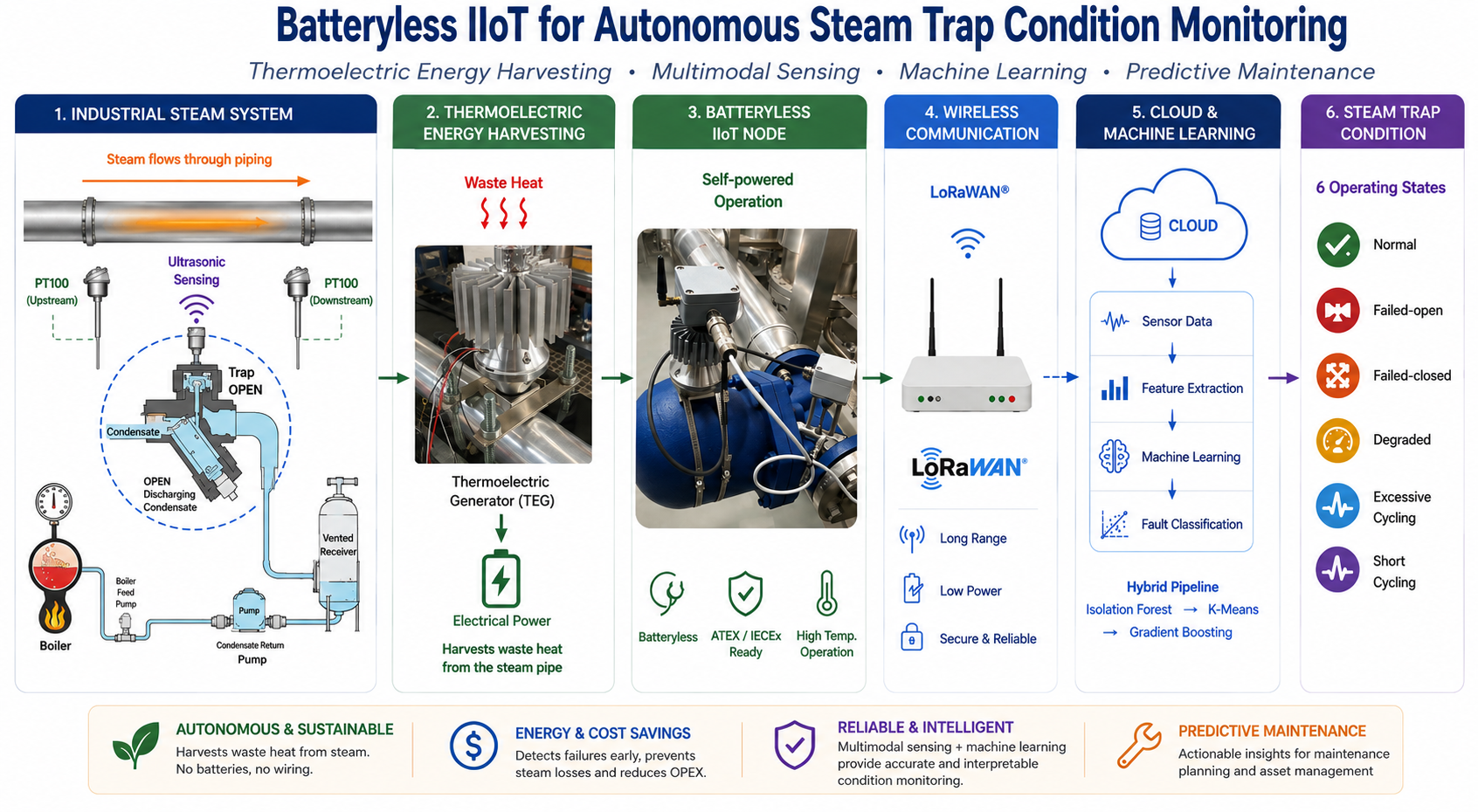
Industrial steam traps can waste energy and increase maintenance requirements when they fail, while continuous monitoring is often constrained by battery life and wiring. This work presents a batteryless Industrial Internet of Things (IIoT) architecture that combines thermoelectric energy harvesting, temperature and ultrasonic sensing, LoRaWAN communication, window-level feature engineering and machine learning for steam-trap condition monitoring. Building on a previously reported heat-powered steam-leak detector, the present study extends the task from binary detec-tion to six operating states: normal, failed-open, failed-closed, degraded, excessive-cycling and short-cycling. The current-scope dataset contains 6,354 windows represented by 117 engineered features. Random Forest, Extra Trees and Histogram-based Gradient Boosting are evaluated using a leakage-reduced feature configuration and chronological testing. Histogram-based Gradient Boosting achieves 0.9958 validation accuracy and 0.9550 validation macro-F1, followed by 0.9853 test accuracy and 0.8822 test macro-F1. A scope-aware deployment strategy restricts formal pre-dictions to supported devices, while later data are used to assess temporal stability. The results show that autonomous multimodal sensing can provide richer condition information than leak/no-leak detection, while highlighting the need for independently verified labels and cross-device validation.
Keywords:
steam trap
; Industrial Internet of Things
; thermoelectric energy harvesting
; energy harvesting
; ultrasonic sensing
; LoRaWAN
; machine learning
; predictive maintenance
; condition monitoring
; steam leakage
1. Introduction
Steam is extensively used in industrial heating, heat transfer, sterilization, cleaning and process operations. Steam distribution systems therefore represent a significant energy infrastructure in sectors [1] such as oil and gas, petrochemical, chemical, pharmaceutical, food processing and power generation. Steam traps are essential components of these systems because they remove condensate and non-condensable gases while retaining live steam. Their correct operation contributes simultaneously to thermal efficiency, process stability and equipment protection.
A malfunctioning steam trap can produce two fundamentally different classes of consequences. A failed-open trap can continuously or excessively discharge live steam, forcing the boiler to generate additional steam and therefore increasing fuel consumption and operating cost [2]. A failed-closed trap can prevent condensate removal, reducing heat-transfer efficiency and potentially contributing to corrosion, unstable operation or water hammer. Between these extreme conditions, traps can exhibit degraded or abnormal cycling behaviour that may be difficult to identify with a single threshold.
The scale of the problem becomes significant because industrial facilities may contain hundreds or thousands of steam traps. That study associated a representative leakage of 0.5 kg/min with approximately 262.8 tonnes of lost steam per year and, using the assumptions adopted in that work, an annual economic impact of approximately EUR 1,314 per leaking trap. The same work highlighted that pressure, orifice size and plant scale can substantially increase the impact. These calculations illustrate why continuous detection is attractive: even a relatively small loss at an individual component can become a major energy and environmental burden when multiplied across a plant.
Traditional steam-trap inspection relies on periodic surveys, handheld ultrasonic instruments, temperature measurements or visual inspection. Such approaches can be effective for targeted maintenance, but they provide only snapshots of system behaviour. Continuous monitoring can instead reveal persistent leakage, intermittent cycling and degradation between inspection campaigns. However, installing large numbers of conventional industrial sensors [3,4] creates two practical barriers: power and infrastructure.
Battery-powered wireless sensors simplify installation but introduce a finite energy budget and periodic maintenance. This issue is particularly relevant when monitoring hundreds of devices or when sensors are installed in difficult-to-access or hazardous areas. Wired instrumentation avoids battery replacement but requires cables, power supplies, switches, gateways and integration infrastructure. A heat-powered architecture [2] can address both limitations by exploiting the temperature difference present in the steam system.
Aragonés et al. [5] previously demonstrated a thermoelectric-generator-powered IIoT device for steam-leak detection. The architecture combined a thermoelectric generator, power conversion, temperature sensing, ultrasonic sensing, edge processing and LoRaWAN communication. The system was designed to operate without a primary battery and to transmit measurements wirelessly over long range. Experimental work demonstrated the feasibility of simultaneously monitoring temperature and ultrasonic activity, although the field test did not contain a confirmed faulty steam trap.
The present work takes the next step. Instead of treating the sensing node [6] only as a leak detector, the collected measurements are converted into structured temporal features and analysed with machine-learning models. The objective is to distinguish multiple operational conditions, thereby providing a richer condition-monitoring output. This is important because maintenance decisions depend not only on whether a trap is abnormal, but also on the nature of the abnormality.
Furthermore, study is positioned at the intersection of three traditionally separate engineering problems. The first is steam-system efficiency, where the objective is to identify abnormal trap behaviour early enough to prevent avoidable steam loss. The second is autonomous industrial sensing, where the objective is to deploy a large number of monitoring nodes without creating a proportional burden in batteries, cabling, power supplies, or maintenance visits. The third is data-driven condition monitoring, where heterogeneous sensor measurements are converted into a repeatable estimate of equipment state. The novelty of the present work lies in treating these three problems as one system rather than optimising them independently.
Hardware performance is therefore discussed in terms of whether the energy source can enable the sensing workload; machine-learning performance is discussed in terms of class balance and temporal stability rather than accuracy alone; and runtime behaviour is discussed in terms of the boundary between supported and unsupported devices. This framing is important for industrial deployment because a classifier with excellent offline accuracy is not necessarily a reliable monitoring system if the sensor cannot operate continuously or if the model is applied outside its training scope. The main contributions of this work are therefore:
- An end-to-end, heat-powered and batteryless IIoT architecture for continuous steam-trap monitoring.
- Integration of thermal, ultrasonic and cycling information into a window-level multimodal feature representation.
- A six-state steam-trap condition-monitoring framework extending beyond binary leak detection.
- A comparison of tree-based machine-learning models under a leakage-reduced feature configuration.
- Chronological and robustness-oriented evaluation designed to better approximate runtime behaviour.
- A scope-aware deployment strategy that prevents unsupported devices or feature distributions from receiving formal diagnostic outputs.
The remainder of the paper is organised as follows. Section 2 describes steam-trap operation and failure modes. Section 3 presents the autonomous IIoT architecture and thermoelectric energy harvesting. Section 4 describes the dataset and feature engineering. Section 5 presents the machine-learning methodology and evaluation design. Section 6 reports the results. Section 7 discusses industrial implications and limitations. Section 8 presents the deployment roadmap and future validation strategy, and Section 9 concludes the paper.
2. Steam Trap Operation, Failure Modes and Monitoring Requirements
2.1. Role and Types of Steam Traps
Steam is widely used in manufacturing industries such as oil and gas, chemicals, pharmaceuticals, and food processing, among other heat-intensive industrial sectors, due to its versatility and efficiency. Steam provides a safer alternative to direct combustion heating, reducing risks of fire and explosions. Major elements involved in steam circuits are:
- Steam boiler. It is the element that converts clean water into steam thanks to several heating elements (electric resistors, fuel, gas, etc).
- Steam pipelines. Their mission is the transportation of steam in all processes.
- Pumps. They are used for pumping water condensed to the boiler.
- Steam traps. In a steam pipeline, they are typically installed every 30 to 50 meters depending on factors like pipe size and operating conditions.
- End of steam pipelines: Steam trap (Figure 1) allows to purge condensate before it re-enters the system.
Steam traps can broadly be grouped into mechanical, thermodynamic and thermostatic devices. Mechanical traps respond primarily to the density difference between steam and condensate. Thermodynamic traps operate through flow and pressure effects and commonly exhibit repeated opening and closing behaviour. Thermostatic traps respond to temperature differences between steam, condensate and non-condensable gases. Consequently, the same measured signal should not necessarily be interpreted identically for all trap types (Table 1).
2.2. Failure Modes
The condition-monitoring framework used in this work defines six engineering states. Normal represents expected behaviour within the supported device scope. Failed-open represents leakage-like or continuously open behaviour and is directly associated with live-steam loss. Failed-closed represents insufficient condensate discharge. Degraded represents intermediate abnormal behaviour that does not clearly correspond to either complete open or complete closed failure. Excessive-cycling and short-cycling describe abnormal dynamic behaviour in the opening and closing process.

Table 2.
Steam trap fails.
| State | Physical interpretation | Typical sensor evidence |
|---|---|---|
| Normal | Expected operating behaviour | Stable thermal response and trap-specific acoustic/cycling pattern |
| Failed open | Continuous or excessive live-steam passage | Hot outlet, persistent ultrasonic activity, loss of normal cycling |
| Failed closed | Blocked or insufficient condensate discharge | Hot inlet/cold outlet tendency, low acoustic activity, absence of expected cycles |
| Degraded | Intermediate abnormal behaviour | Irregular temperature, acoustic or cycling patterns |
| Excessive cycling | Higher-than-expected cycle activity | Elevated pulse/cycle frequency |
| Short cycling | Rapid repeated cycles over short intervals | Rapid pulse activity and characteristic acoustic pattern |
These states should be interpreted as condition-monitoring indicators rather than direct maintenance work orders. In particular, degraded and cycling-related states may overlap with normal behaviour depending on trap technology and operating conditions. Final maintenance decisions should incorporate plant context, device history and, where possible, field confirmation.
2.3. Environmental and Economic Motivation
Steam leakage has a direct environmental consequence because the lost steam must generally be replaced by additional boiler production. The resulting fuel consumption depends on boiler efficiency, steam pressure, feedwater conditions and fuel type. The earlier experimental work used a representative leakage scenario to illustrate the scale of the problem. A common oil&gas refinery with thousands of traps can therefore accumulate substantial avoidable energy use. Continuous monitoring is attractive because it can reduce the time between fault occurrence and maintenance intervention.
The environmental argument also applies to the monitoring infrastructure itself. A batteryless architecture avoids recurring battery replacement and associated logistics, while thermoelectric harvesting reuses heat already present in the process. The overall sustainability benefit is therefore a combination of avoided process losses and reduced sensor-maintenance burden.
The research gap is therefore the integration of (i) process-heat-powered sensing, (ii) multimodal thermal and acoustic observation, (iii) long-range IIoT communication, and (iv) scope-aware multi-state machine learning in one monitoring workflow. This combination is intended for distributed industrial assets where battery replacement and wired instrumentation can become significant lifecycle constraints.
The present work addresses a complementary problem: how to obtain continuous multimodal data autonomously while extending the analytical output from leakage detection to a defined six-state condition-monitoring framework. Unlike approaches that assume externally powered sensor infrastructure, the proposed workflow couples process-heat-powered sensing with long-range IIoT communication and a scope-aware machine-learning layer.
Recent work confirms growing interest in data-driven steam-trap monitoring. Acoustic-emission and ultrasonic methods remain attractive because they provide information about internal flow and leakage that cannot always be inferred from temperature alone. Recent machine-learning approaches have also moved toward richer fault-diagnosis pipelines using time-series features and deep models, demonstrating that steam-trap diagnosis is becoming a data-intensive sensing problem [7,8].
2.4. Physicalsignatures Ofsteam Trap States
The physical observability of a steam-trap condition depends on the interaction between temperature, flow, pressure and valve dynamics. Under normal operation, the trap removes condensate while limiting live-steam passage. The upstream and downstream thermal conditions therefore differ according to the trap design and process operating point. When a trap remains open, the downstream side can approach the upstream thermal condition because steam passes continuously through the device. Conversely, a blocked or closed trap can cause condensate accumulation and a reduction in the expected downstream thermal response.
Temperature alone is not always sufficient to distinguish these states. Hot condensate can undergo flashing after a pressure reduction, producing thermal conditions that resemble steam flow. The previous experimental work therefore combined inlet/outlet PT100 measurements with ultrasonic sensing. It reported that ultrasonic activity around the 30–40 kHz region was useful for identifying steam leakage while avoiding part of the industrial noise observed at lower frequencies. The ultrasonic microphone used in the prototype had a 50 kHz bandwidth and the acquisition stage operated at 160 kHz sampling. This multimodal principle motivates the feature design in the present study. Rather than asking one sensor to identify a failure, the machine-learning model receives complementary evidence: thermal level and difference, acoustic intensity and spectral behaviour, and temporal pulse or cycling activity. The expectation is not that every feature is useful for every class. Instead, the combination should provide a richer representation in which different physical signatures become available to the classifier.
3. Materials and Methods: Autonomous Thermoelectric IIoT
3.1. System Overview
Accordingly with Figure 2, the proposed architecture is based on five functional layers. The first is the energy and sensing layer attached to the steam system within the embedded IIoT layer, which conditions the sensor signals, performs local processing and communicates through LoRaWAN. The third one is the LoRaWAN gateway. The fourth is the cloud platform for data-analysis layer, where temporal windows are transformed into features and evaluated by the machine-learning pipeline. Last layer is the visualization interface.
The node is intended to be installed externally, avoiding intrusive modifications to the steam path. The temperature interface provides thermal information while the ultrasonic channel provides information about high-frequency flow activity. The architecture can additionally use pulse or cycle indicators derived from the acoustic signal. This combination is important because no single physical variable fully describes all steam-trap states.
3.2. Thermoelectric Energy Harvesting
This module, based on TEG power converter system presented in allows the heat to electricity conversion thanks to a thermal model system that permits a constant DC output voltage (5V) independently of the surface temperature. This subsection summarizes thermoelectric tests performed in that paper for a better understanding of the solution.
All tests were conducted entirely in AEInnova’s laboratory, a spin-off of the Microelectronics Department at the Autonomous University of Barcelona (Figure 3), where the authors of this paper are principal founders. This job was done during last quarter of 2024. For the complete characterization, a test bench was developed, consisting of a 2-inch pipeline heated by a 150W resistor and a support structure for the pipeline. The test bench includes a PID controller and a precise PT100 temperature sensor to ensure accurate temperature control of the pipeline surface. For the measurements, the temperature was increased in 10 °C increments, with a 20-minute stabilization period for the thermoelectric generator (TEG) surface temperature at each step.
The energy source is the temperature difference between the hot steam system and the surrounding environment. A thermoelectric generator converts part of this thermal gradient into electrical energy through the Seebeck effect. The usable electrical power depends on the thermoelectric material, hot- and cold-side temperatures, thermal interfaces, heat-sink design and electrical operating point.
The previously reported architecture used a dedicated thermoelectric module coupled to a thermal interface and radiator. Characterization showed that the open-circuit voltage increased with source temperature and temperature difference. In the reported experiments, the system was designed to supply the embedded electronics and sensors without a primary battery. The power-management stage includes DC/DC conversion and energy storage, allowing intermittent sensing and radio transmission even when instantaneous harvested power is lower than the peak system demand. Power generation results are presented in Figure 4. Table 3 summarizes thermoelectric performance.
A key design principle is therefore energy-aware duty cycling. Sensing, feature extraction and communication are scheduled so that the average energy demand remains compatible with the available harvested energy. A supercapacitor can buffer the difference between slow thermal energy accumulation and short communication bursts.
3.2.1. Thermoelectric Conversion Model
For a first-order representation, the open-circuit voltage generated by a thermoelectric generator can be expressed as:
VOC ≈ Seff * ΔT (1)
where Seff is the effective Seebeck coefficient of the module and ΔT is the temperature difference between the hot and cold sides.
Under load, the delivered electrical power depends additionally on the internal electrical resistance and the operating point imposed by the power-management circuit. The maximum-power condition is therefore not equivalent to the open-circuit-voltage condition.
The previous steam-trap study characterized the TEG on a 2-inch heated pipe test bench using a 150 W resistor, a PID controller and a PT100 reference. The hot-side temperature was increased in 10 °C increments with approximately 20 min stabilization at each step. Measurements covered hot-side temperatures from 50 °C to 170 °C and ambient temperatures from 15 °C to 40 °C. The maximum reported open-circuit voltage was 3.687 V at 170 °C hot-side temperature and 15 °C ambient temperature. The maximum reported generated power was 1.034 W under the same condition.
These results are important for the present paper for a reason that goes beyond the peak power value. The ML system requires repeated acquisition, feature extraction and wireless transmission. A process that can provide a sustained temperature gradient can therefore act as the energy budget for the complete sensing pipeline. In opposition, the relevant deployment quantity is the minimum sustainable harvested power under the actual thermal installation, not the maximum laboratory power. The distinction should be retained when moving from laboratory characterization to field deployment.
3.2.2. Energy Budget and Duty-Cycled Operation
The autonomous node should be analyzed as an energy-balance problem. Let P_H be the average harvested electrical power, P_S the average sensing power, P_E the embedded-processing power, P_C the average communication power and P_L the losses in power conversion and storage. A sustainable operating point requires:
P_H ≥ P_S + P_E + P_C + P_L (2)
Because communication is burst-like, the supercapacitor or storage element decouples the instantaneous radio demand from the slower thermal harvesting process.
This architecture also changes the design logic of the ML system. A conventional powered sensor may acquire raw waveforms continuously and transmit large data volumes. A heat-powered node cannot assume the same energy budget. Feature engineering therefore becomes an architectural function: the node can reduce high-rate measurements to compact descriptors and communicate those descriptors rather than continuous raw signals. The resulting system simultaneously reduces radio energy and creates a structured dataset suitable for tabular machine learning.
The previous implementation transmitted data approximately every five minutes and used LoRaWAN as the long-range communication mechanism. The present paper does not claim that this interval is universally optimal; rather, it demonstrates the principle that the sensing workload and communication schedule must be designed together with the available thermal energy.
3.2.3. Acoustic and Ultrasonic Observation
Ultrasonic sensing provides a complementary observation channel because high-frequency acoustic energy can be associated with turbulent or high-velocity flow through the trap. The prototype used a 50 kHz-bandwidth ultrasonic microphone. Because the microphone membrane is sensitive to temperature, the mechanical implementation separated the microphone from the hot trap and used an aluminium waveguide to transfer acoustic energy while reducing the thermal exposure. This mechanical detail is relevant to autonomous sensing because sensor survivability is part of the overall system reliability. The previous experiments showed that the acoustic signal could reveal leakage episodes that were not sufficiently unambiguous from temperature alone. In particular, the manuscript reports a characteristic response around 37 kHz and therefore focuses on a 30–40 kHz band to reduce interference from lower-frequency industrial noise. In the present ML pipeline, the acoustic signal is not treated as a single threshold. Its RMS level, band ratio, peak value, peak frequency and temporal statistics are transformed into features, allowing the model to learn combinations of acoustic and thermal evidence.
4. Materials and Methods: Data Acquisition and Feature Engineering
4.1. Device Scope and Dataset
The machine-learning dataset used in this study contains 6,354 window-level records and 117 candidate features for the current-scope device population. The records are derived from sensor measurements collected by steam-trap monitoring devices during 8 months (August 2025-March 2026) in one pharma ficility of located in Barcelona. The current-scope population is deliberately separated from legacy and out-of-scope devices because sensor availability, feature distributions and device behavior are not necessarily identical.
The data is divided into 4,449 training windows, 954 validation windows and 951 test windows. The training set is used to fit candidate models, the validation set supports model selection and the test set is reserved for final evaluation. In addition to aggregate metrics, chronological evaluation is used to examine performance on later data.
4.2. Window-Level Representation
Continuous sensor streams are transformed into analysis windows. Each window is represented by a set of descriptive variables that capture thermal level and variation, acoustic activity and spectral characteristics, pulse and cycling behaviour, and statistical properties. This representation reduces the dimensionality of continuous sensor streams while preserving information relevant to operating state.
4.2.1. Temporal Window Rationale
A window-level sample is preferable to treating every raw measurement as an independent observation because steam-trap behavior is dynamic. A single temperature can be compatible with several operating conditions, whereas a sequence can reveal a stable level, repeated pulses, a gradual thermal drift, or a transition between states. The thesis explicitly [9] defines each analysis window as one machine-learning sample and extracts temperature, acoustic, pulse and statistical descriptors from that interval.
Windowing also reduces the computational and communication burden of the batteryless node. Instead of transmitting every sample of a high-rate ultrasonic waveform, the embedded system can compute summary quantities such as RMS, band ratios, peaks and pulse counts. This creates a hierarchy: high-rate physical sensing at the edge, compact feature representation at the node, and multi-state interpretation in the machine-learning layer.
The correct window duration is therefore a trade-off. Very short windows may miss the temporal context required to distinguish cycling patterns; very long windows can delay detection and blur transitions. The present study uses the window structure defined by the thesis dataset and does not claim that one window length is universally optimal. Future experiments should evaluate the effect of window duration explicitly, especially for early-warning detection.
4.2.2. Feature Taxonomy and Physical Meaning
The feature table contains several distinct information families. Temperature variables include direct measurements and derived quantities such as inlet temperature, outlet temperature, ΔT and absolute ΔT. Acoustic variables include RMS, mean RMS, band ratio, peak value and peak frequency. Pulse and cycling variables represent the dynamic activity of the trap. Statistical features summaries the distribution within each window using quantities such as mean, standard deviation, minimum, maximum, range and rolling statistics. Metadata and quality variables describe device context and feature availability.
This taxonomy is important because it allows the ML model to combine variables with different physical roles. Thermal variables describe the state of the process, acoustic variables describe flow-related activity, dynamic variables describe temporal behavior, and metadata variables describe the measurement context. The model is therefore not simply learning a threshold in temperature space; it is learning a nonlinear decision surface across several physical and contextual dimensions.
At the same time, metadata must be handled carefully. Device identifiers and routing variables can be highly predictive of the target without representing physical behavior. Such variables are precisely why leakage-reduced feature selection is necessary. A high-performing industrial model should rely primarily on variables that remain meaningful when the device population or operating context changes.
Table 4.
ML parameters.
| Feature group | Examples | Physical information |
|---|---|---|
| Temperature | temperature, inlet temperature, outlet temperature, ΔT, |ΔT| | Thermal state and thermal balance |
| Ultrasound/acoustic | RMS, mean RMS, band ratio, peak value, peak frequency | Flow and leakage-related acoustic activity |
| Pulse/cycling | pulse count, pulse frequency, mean/std pulses | Dynamic opening/closing behaviour |
| Statistical windows | mean, standard deviation, minimum, maximum, range, rolling statistics | Short-term operating variability |
| Metadata / quality | device ID, mode, diagnostics, missing-value flags | Data validity and device context |
4.3. Why Multimodal Features Matter
The six-state problem is inherently multimodal. Temperature provides information about the thermal condition but may not uniquely identify flow behavior. Ultrasound captures internal flow and leakage activity but can be affected by installation and environmental noise. Cycling information describes temporal behavior but must be interpreted in relation to trap type. Combining these modalities allows the classifier to identify patterns that are not represented by a single threshold.
This is also a central advantage of the proposed IIoT architecture. Because the node is autonomous and continuously connected, the system can build a temporal history rather than relying on a single measurement campaign. That history provides the basis for window-level feature engineering and temporal evaluation.
5. Materials and Methods: Machine Learning Methodology
5.1. Problem Formulation
The condition-monitoring task is formulated as a supervised six-class classification problem. For each analysis window x, the model estimates a class y belonging to the set {normal, failed-open, failed-closed, degraded, excessive-cycling, short-cycling}. The objective is not simply to maximize overall accuracy, but to obtain stable class-level behavior suitable for runtime monitoring.
The distinction between a classification model and a maintenance decision is important. The model predicts an engineering condition category from sensor-derived evidence. It does not directly determine whether a valve should be replaced. This separation reduces the risk of presenting a probabilistic model output as a definitive maintenance diagnosis.
5.1.1. Engineering Labels Versus Ground Truth
The most important methodological qualification in the present study concerns the target labels. The six classes are engineering condition categories generated from sensor-derived operational rules. The thesis explicitly states that they should be interpreted as model output classes rather than direct maintenance work orders, and that final maintenance decisions require field information, device history and expert inspection when available.
This distinction changes the interpretation of the reported accuracy. A test accuracy of 98.53% means that the classifier agrees with the evaluation labels for 98.53% of the test windows; it does not mean that 98.53% of field failures have been independently diagnosed correctly. The paper therefore uses the term ‘condition-state classification’ rather than claiming validated fault-diagnosis accuracy. This is not a weakness to conceal. It is a central research-design issue and an opportunity for the next experimental phase. Once maintenance records, field inspections, or controlled fault tests become available, the current engineering-label framework can be evaluated against independent outcomes. The resulting experiment would distinguish agreement with the operational taxonomy from true diagnostic validity.
5.1.2. Leakage Risk and Causal Interpretation
Label leakage occurs when a feature contains information that would not legitimately be available at prediction time or directly encodes the rule used to construct the target. In the present dataset, the risk is particularly relevant because the six states are engineering-rule-based. Direct label fields, previous prediction outputs, routing indicators and high-risk proxy variables can therefore create an artificial shortcut for the classifier.
The thesis addresses this issue by defining a non-strict leakage-reduced configuration with 108 features and a stricter configuration with 81 features. The non-strict setting removes direct label-related, prediction-related, routing-related and high-risk rule-derived variables while preserving informative physical and statistical features. The strict setting removes an additional group of potential proxies.
The resulting performance difference is scientifically informative. If performance were unchanged after aggressive removal, confidence that the model relied on physical information would increase. Instead, macro-F1 decreases substantially under the strict setting. The correct conclusion is therefore that the engineered feature space contains valuable information but that some of the retained information may still be closely coupled to the labelling process. Independent labels are required to resolve this ambiguity.
5.2. Label Generation and Its Consequences
The available labels are engineering, rule-informed pseudo-labels generated from the combined interpretation of temperature, acoustic and cycling signals. They are therefore not equivalent to independently verified ground-truth failure records. Failed-open and failed-closed patterns are generally more physically interpretable, whereas degraded and cycling-related states are more difficult to separate.
This characteristic creates an important machine-learning risk: if the feature set contains variables that directly encode the rules used to generate the labels, a model can achieve very high numerical performance without learning a sufficiently general physical relationship. To address this, the advanced model-development stage removes direct label-related, prediction-related and high-risk rule-derived variables. This is referred to as the leakage-reduced configuration.
5.2.1. Why Tree-Based Models
Tree-based models were selected because the input is a structured tabular representation containing nonlinear interactions, mixed scales and potentially correlated variables. Unlike linear models, tree ensembles can represent threshold-like effects and interactions without requiring an explicit physical equation for every class boundary. They also avoid the need for extensive normalization when features have different units or distributions.
Random Forest provides [10] a strong ensemble baseline through bootstrap sampling and randomized feature selection. Extra Trees increases randomization in the construction of the individual trees [11]. Histogram-based Gradient Boosting instead builds an additive sequence of trees in which later learners focus on residual classification errors [12]. The latter is particularly suitable when a compact feature representation contains nonlinear interactions that can be refined iteratively.
The comparison is therefore not intended as an exhaustive ML benchmark. It is a controlled comparison of three interpretable, deployment-friendly tree approaches that fit the current tabular data representation. More complex deep-learning models may become relevant when larger raw time-series datasets are available, but they would also introduce greater requirements for data volume, validation, compute resources and explainability.
5.2.2. Model Selection Criteria
Model selection is based on four criteria: predictive performance, class-level balance, temporal stability and deployment suitability. Accuracy is retained because it provides an intuitive overall measure. Macro-F1 is given greater importance because it weights the classes equally and therefore reveals whether a model performs poorly on minority states. Temporal stability is assessed using the chronological 70/15/15 split. Finally, the model must operate within the defined current-scope feature schema and support the runtime routing strategy.
This multi-criteria selection is preferable to choosing the model with the highest training accuracy. The training score is particularly uninformative when labels are structured and the model has access to many engineered features. The final model should instead demonstrate that performance remains strong after leakage reduction and when evaluated on later data.
5.3. Candidate Models
Three tree-based classifiers are evaluated: Random Forest, Extremely Randomized Trees and Histogram-based Gradient Boosting. Tree ensembles are appropriate for the structured tabular feature representation because they can model nonlinear interactions without requiring the signal distributions to be transformed into a linear form.
Random Forest constructs an ensemble of decision trees using bootstrap sampling and feature randomization. Extremely Randomized Trees increase randomization in the tree construction process. Histogram-based Gradient Boosting builds an additive sequence of trees, where later trees focus on errors made by previous trees. The latter can efficiently model nonlinear interactions in a relatively high-dimensional tabular feature space.
Table 5.
Model test.
| Model | Validation accuracy | Validation macro-F1 | Test accuracy | Test macro-F1 |
|---|---|---|---|---|
| Random Forest | 0.9717 | 0.8030 | 0.9581 | 0.7267 |
| Extra Trees | 0.9496 | 0.7171 | 0.9403 | 0.4810 |
| Histogram Gradient Boosting | 0.9958 | 0.9550 | 0.9853 | 0.8822 |
For a given class, precision measures the fraction of predicted positives that are correct, while recall measures the fraction of actual class instances that are recovered. The F1-score combines both quantities. Macro-F1 is calculated as the unweighted mean of the class-level F1 scores. This makes it particularly relevant when some states occur much less frequently than others.
The distinction between weighted and macro metrics is central to this application. A failed-open or degraded state may dominate the available windows, while excessive-cycling and short-cycling may be comparatively rare. A classifier could therefore obtain high accuracy while almost ignoring one of the minority classes. Macro-F1 prevents the majority classes from completely masking this behavior.
Confusion matrices are equally important because they identify physically meaningful error boundaries. Confusion between failed-open and failed-closed would be operationally significant. Confusion between excessive cycling and short cycling is different: both represent dynamic abnormalities and may have overlapping physical signatures. The final interpretation therefore combines aggregate scores with the engineering meaning of each error.
5.4. Evaluation Metrics
Accuracy is calculated as the fraction of correctly classified windows. Because the six classes are not equally represented, accuracy alone is insufficient. Precision, recall and F1-score are therefore calculated at class level. For a class, precision is TP/(TP+FP), recall is TP/(TP+FN), and F1 is the harmonic mean of precision and recall. Macro-F1 is the arithmetic mean of the six class-level F1 values and gives equal weight to each class.
Confusion matrices are used to identify which states are systematically confused. This is particularly relevant for degraded, excessive-cycling and short-cycling states, where the physical boundaries may be less distinct than for failed-open or failed-closed conditions.
Temporal evaluation is designed to approximate a real deployment sequence in which the model is trained on historical data and then receives later observations. The thesis uses the first 70% of records for training, the next 15% for validation and the final 15% for testing.
This design does not eliminate all forms of temporal dependence, because adjacent windows may still be related. Nevertheless, it is more informative than a random split when the objective is to test stability under later operating conditions. It can reveal changes caused by maintenance events, sensor drift, process changes or variations in the trap population.
A particularly important result is that the later validation and test blocks do not contain all six classes. Normal and failed-closed are absent from those later blocks. Therefore, the temporal experiment cannot be interpreted as complete six-class validation over time. Instead, it demonstrates that the selected model remains stable for the states represented in the later periods. This limitation should remain explicit in the paper.
5.5. Temporal Evaluation
Random splits can produce optimistic estimates when neighboring windows from the same temporal process appear in both training and test data. For deployment-oriented evaluation, the selected model is therefore also evaluated using chronological blocks. The current implementation uses the first 70% of the records for training, the following 15% for validation and the final 15% for testing.
The purpose of the time-block evaluation is not only to obtain a second accuracy number. It tests whether the learned relationship remains stable when the model is exposed to later observations. Changes in operating conditions, device behavior, maintenance events and sensor quality can produce temporal drift. A model that performs well only under a random split may therefore be unsuitable for continuous industrial deployment.
Scope-aware routing is a key part of the proposed methodology rather than software convenience. The training distribution is defined by the current device population and feature schema. Legacy variants may have different sensor availability or feature distributions, while out-of-scope records may be structurally incompatible with the classifier. Applying the same model to all records would therefore create an implicit assumption of distributional equivalence that has not been demonstrated.
The runtime architecture distinguishes three paths. Current-scope records proceed to formal six-state predictions. Legacy records can be processed through shadow inference for exploratory comparison, but their outputs are not treated as formal diagnoses. Out-of-scope records are rejected from formal predictions. The thesis demonstrates this routing on 23,684 window-level records, of which only 6,354 were in current scope.
This conservative design is especially appropriate for industrial AI because a system should be able to say ‘unsupported’ rather than generate a confident output outside the distribution for which it was evaluated. In a production system, this mechanism could be extended with automated drift detection, feature-schema monitoring and model-version qualification.
5.6. Scope-Aware Runtime Strategy
The runtime pipeline separates devices into three groups. Current-scope devices have the feature structure and signal behavior used for formal model development. Legacy devices can be processed through shadow inference for exploratory analysis but do not receive formal six-state outputs. Out-of-scope devices are rejected from formal diagnosis.
This mechanism is deliberately conservative. A machine-learning model should not be applied to an input distribution for which its training data provides no evidence of validity. In industrial monitoring, a transparent ‘not supported’ output is preferable to a confident but unsupported fault classification.
5.7. Post-Processing and Runtime Interpretation
The runtime workflow can apply conservative post-processing after the base model prediction. The purpose is to avoid over-interpreting ambiguous predictions and to maintain a clear distinction between model output and maintenance action. The dashboard representation includes prediction status, device scope and supporting metadata, allowing operators to inspect the context of each output.
5.8. Software, Reproducibility and Deployment Controls
The machine-learning pipeline was implemented in Python 3.13.5 using scikit-learn 1.8.0. Numerical missing values were imputed using the median, categorical missing values using the most frequent category, and categorical variables were ordinal-encoded with unseen categories assigned a value of −1. A random state of 42 was used for model training. The same preprocessing pipeline and feature schema were maintained across training, validation, testing, and runtime inference. The implementation code, trained-model package, scope-routing configuration, post-processing rules, and dashboard are publicly available at:
5.9. Feature-Group Interpretation and Error Analysis
The classifier should be interpreted as a multimodal model rather than an acoustic-only or temperature-only detector. Thermal features provide slow process context; ultrasonic features provide sensitivity to flow and leakage dynamics; and pulse/cycling features describe opening and closing behavior. The engineered representation therefore converts high-rate physical signals into compact variables with direct engineering meaning.
The main classification difficulty was observed between the cycling-related classes, particularly excessive cycling and short cycling. In the chronological evaluation, failed-open remained comparatively stable and degraded retained high recall, whereas greater confusion occurred between excessive cycling and short cycling. This behavior is consistent with the dynamic and partially overlapping characteristics of these operating states.
6. Results
All tests were conducted in the pharma facility in Barcelona during Agust 2025 -March 2026. Equipment and installation are shown in Figure 5.
The numerical comparison shows a clear separation between the candidate models. Random Forest reaches 0.8030 validation macro-F1 and 0.7267 test macro-F1, while Extra Trees reaches 0.7171 and 0.4810, respectively. Histogram-based Gradient Boosting reaches 0.9550 validation macro-F1 and 0.8822 test macro-F1. The same ordering is observed in accuracy, with HistGradientBoosting achieving 0.9958 validation accuracy and 0.9853 test accuracy.
The difference in macro-F1 is more important than the difference in accuracy. Extra Trees, for example, retains a relatively high overall test accuracy of 0.9403 while its test macro-F1 falls to 0.4810. This indicates that the model can classify a substantial number of majority-class windows correctly while failing to maintain balanced performance across the six-state taxonomy. HistGradientBoosting shows a much smaller gap between accuracy and macro-F1 and is therefore the stronger candidate for a condition-monitoring application.
The result also provides a practical reason for preferring gradient boosting over the other two models in the current dataset. The feature representation contains nonlinear combinations of thermal, acoustic and dynamic variables. Sequential boosting can refine decision boundaries around difficult regions, whereas the randomized tree ensembles appear less effective at preserving minority-class performance.
6.1. Model Comparison
Histogram-based Gradient Boosting clearly outperformed the other candidate models under the leakage-reduced configuration. Its validation macro-F1 of 0.9550 was substantially higher than Random Forest at 0.8030 and Extra Trees at 0.7171. The difference was also maintained in the chronological test period, where the three models achieved macro-F1 values of 0.8822, 0.7267 and 0.4810, respectively (Figure 6).
The result is important because macro-F1 penalizes models that perform well on dominant classes but poorly on minority classes. For a steam-trap monitoring application, correct classification of a less frequent abnormal state can be operationally more valuable than achieving a marginal increase in overall accuracy on the majority class.
The time-block results show a gradual reduction from the training period to the later test period: accuracy changes from 1.0000 to 0.9958 and then 0.9853, while macro-F1 changes from 1.0000 to 0.9550 and then 0.8822. The decline is expected when the model is evaluated on later observations, but the absolute test performance remains high for the classes represented in the test block.
The more informative observation is the class-specific error pattern. The thesis reports that failed-open remains highly stable and degraded also retains high recall, whereas excessive cycling and short cycling are more frequently confused [9]. This behavior has a physical interpretation: complete open or degraded states can create more persistent signatures, while cycling states are defined by temporal behavior that may overlap between categories.
The chronological test should therefore be interpreted as evidence of useful temporal stability rather than proof of universal generalization. The absence of normal and failed-closed from the later blocks means that those two classes are not being challenged under the same temporal conditions. A future dataset containing long, continuous records from all six states would allow a much stronger temporal experiment.
6.2. Time-Block Performance
The selected model maintained high accuracy in the final chronological block, although macro-F1 decreased relative to validation. The reduction is mainly associated with the more difficult separation of cycling-related conditions. Failed-open behaviour remained comparatively stable, while degraded behaviour was also classified with high recall. Excessive-cycling and short-cycling showed greater confusion, which is physically plausible because both represent dynamic operating conditions rather than clearly separated static states (Figure 7 and Table 6).
An additional limitation of the temporal experiment is that the later blocks do not contain all six operating states. In particular, normal and failed-closed samples are absent from the later chronological blocks. Consequently, the temporal results demonstrate stability for the classes represented in those periods but cannot be interpreted as equal temporal validation of all six states.
The robustness experiment is arguably more informative than a small increase in headline accuracy because it probes how dependent the classifier is on the feature construction. In the non-strict configuration, 108 features are retained and the selected model achieves 0.9550 validation macro-F1 and 0.8822 test macro-F1. Under the strict 81-feature configuration, validation macro-F1 falls to 0.6307 and test macro-F1 to 0.4999.
The fact that accuracy remains 0.9361 in the strict test while macro-F1 falls to 0.4999 is especially revealing. It shows that accuracy alone would substantially overstate the robustness of the classifier. The model still recognises many majority-class windows, but its ability to separate smaller or more difficult states deteriorates.
The strict experiment should therefore be presented as a credibility analysis rather than as a competing final model. It demonstrates both that the feature representation contains genuine predictive information and that the current label/feature construction is not yet sufficient to establish fully causal physical diagnosis. The next step is not simply to add more features, but to identify which features remain predictive against independently verified labels.
6.3. Robustness and Leakage Reduction
The robustness analysis compares a non-strict leakage-reduced configuration containing 108 features with a stricter 81-feature configuration. The strict configuration removes additional variables considered potentially related to label-generation rules. Performance decreases under this restriction, demonstrating that the feature set contains information that materially supports classification (Figure 8).
This result has two interpretations. First, it confirms that the multimodal feature representation is informative. Second, it highlights the need to distinguish genuine physical predictors from variables that may act as proxies for the rule-based labelling process. The result therefore supports further work on physically grounded feature selection and independently verified labels.
The runtime experiment processed 23,684 records. Only 6,354 (26.8%) were eligible for formal six-state prediction, while 4,511 (19.0%) were retained as legacy shadow records and 12,819 (54.1%) were rejected from formal prediction.
The result is operationally important. More than half of the available records would have been outside the formal model boundary. A deployment architecture that ignored scope would therefore have generated a large volume of predictions without evidence that the feature distribution was compatible with the trained model. The routing mechanism converts this limitation into an explicit system state.
The scope distribution also suggests a roadmap for future model development. Legacy records are not necessarily useless; they form a pool for future domain adaptation or retraining. However, they should first be characterised, labelled and validated before being merged into the formal training population. Similarly, the out-of-scope pool can reveal which sensor or feature changes most limit model portability.
6.4. Runtime Scope Distribution
The runtime demonstration processed 23,684 window-level records. Of these, 6,354 belonged to the current model scope, 4,511 belonged to the legacy variant pool and 12,819 were classified as out of scope. Consequently, only 26.8% of all processed records received formal six-state outputs, 19.0% were retained for shadow analysis and 54.1% were rejected from formal prediction (Figure 9).
Table 7.
Process’ results.
| Runtime category | Records | Share |
|---|---|---|
| Current scope / formal prediction | 6,354 | 26.8% |
| Legacy / shadow inference | 4,511 | 19.0% |
| Out of scope / rejected | 12,819 | 54.1% |
| Total | 23,684 | 100% |
The high proportion of out-of-scope records is not a failure of the classifier; it demonstrates why scope-aware routing is necessary. Applying the model indiscriminately to all records would have generated unsupported outputs for more than half of the runtime dataset.
The formal prediction distribution contains 2,619 degraded windows, 1,625 failed-open windows, 1,372 failed-closed windows, 455 normal windows, 165 short-cycling windows and 118 excessive-cycling windows. The distribution is therefore strongly concentrated in the degraded and complete-failure categories, while dynamic cycling states are comparatively rare.
This distribution should not be interpreted as the prevalence of failure in an industrial plant. It reflects the composition of the available runtime dataset, the current device scope and the windowing process. Nevertheless, it demonstrates that the model can generate a richer condition vocabulary than a binary leak detector.
From a maintenance perspective, the six outputs can be grouped into different response priorities. Failed-open is directly associated with potential live-steam loss and therefore energy and emissions impact. Failed-closed is more closely associated with condensate-management risk. Degraded can be used as a trend or early-warning category, while excessive and short cycling can trigger closer observation or inspection. This interpretation should remain advisory rather than prescriptive until the model is validated against maintenance outcomes.
6.5. Formal Six-State Distribution
The formal outputs are dominated by degraded, failed-open and failed-closed states, while cycling-related states occur less frequently. This distribution should not be interpreted as a plant-level failure prevalence because the dataset composition and current device scope influence the available windows. It is instead evidence that the runtime pipeline can distinguish multiple operating categories within its supported scope.
Figure 10.
Distribution of formal six-state predictions for the 6,354 current-scope runtime records.
Figure 10.
Distribution of formal six-state predictions for the 6,354 current-scope runtime records.
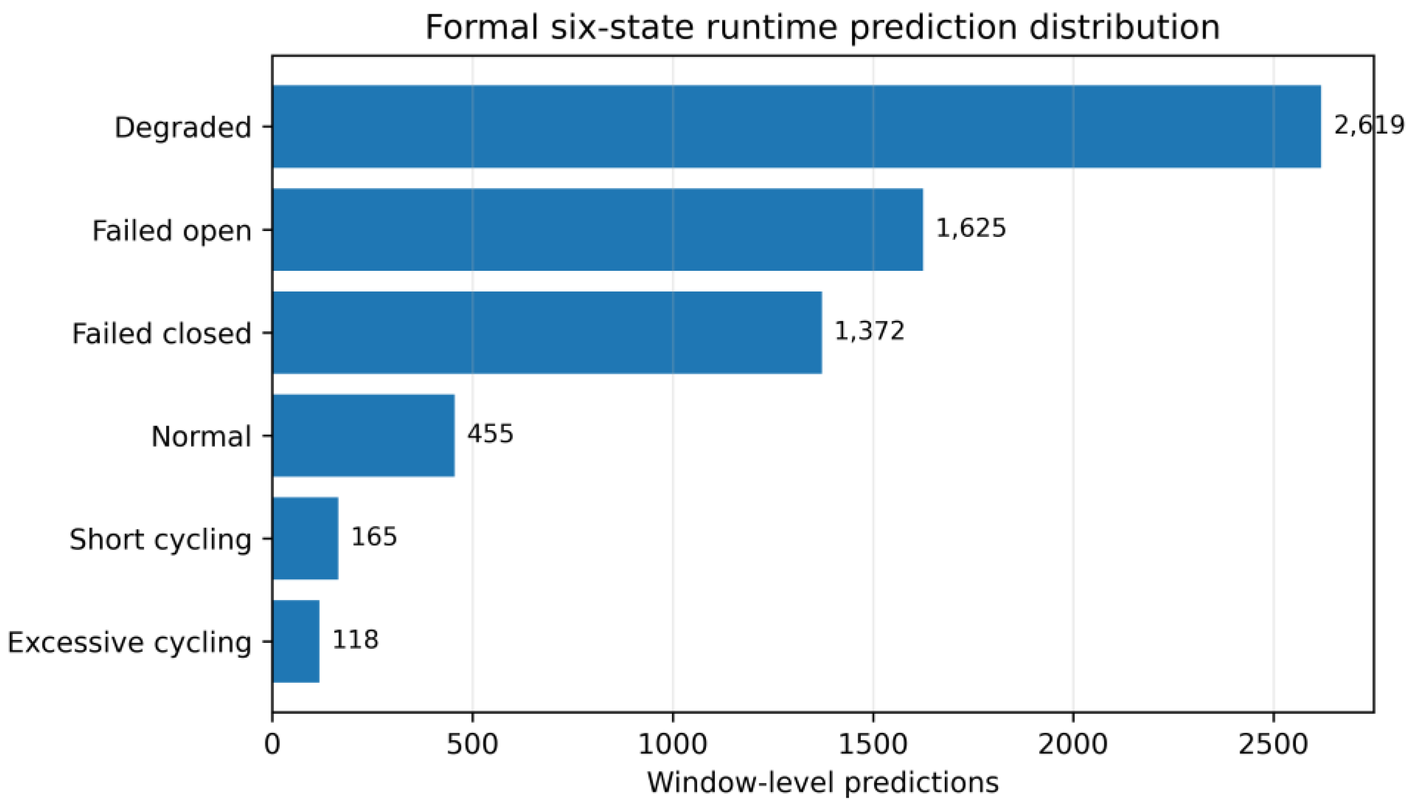
Table 8.
Model’s detections.
| Predicted state | Windows |
|---|---|
| Degraded | 2,619 |
| Failed open | 1,625 |
| Failed closed | 1,372 |
| Normal | 455 |
| Short cycling | 165 |
| Excessive cycling | 118 |
6.6. Runtime Dashboard and Device-Level Visualization
The runtime dashboard provides the final human-facing layer of the proposed monitoring architecture. Rather than presenting the machine-learning output as an isolated class label, the prototype exposes the data-loading status, model scope, prediction status and device-level information required to interpret the result. The thesis prototype processes the scope-aware runtime output and distinguishes formal current-scope predictions from legacy shadow inference and rejected out-of-scope records (Figure 11).
The overview screen gives an immediate indication of whether the runtime dataset is being processed as expected. It reports the total number of windows together with the number receiving formal predictions, legacy shadow outputs and rejected out-of-scope records. In the demonstrated run, 23,684 windows were processed, of which 6,354 were current-scope records, 4,511 were legacy and 12,819 were out of scope (Figure 11). This view is useful from an industrial-operations perspective because it makes model qualification visible before individual predictions are interpreted.
The Device Explorer moves from fleet-level monitoring to asset-level inspection. For a selected device, the prototype displays the number of available windows, model and scope status, mean prediction confidence and the distribution of the six condition states. This is particularly valuable for maintenance-oriented interpretation because a single instantaneous classification can be misleading, whereas the distribution across many windows reveals whether an asset is predominantly normal, degraded, failed or cycling (Figure 12). The thesis identifies this device-level inspection as a specific dashboard function.
Figure 13.
Device-level time-series feature inspection view, showing selected temperature and acoustic/derived features over time for visual interpretation of the model inputs [4].
Figure 13.
Device-level time-series feature inspection view, showing selected temperature and acoustic/derived features over time for visual interpretation of the model inputs [4].
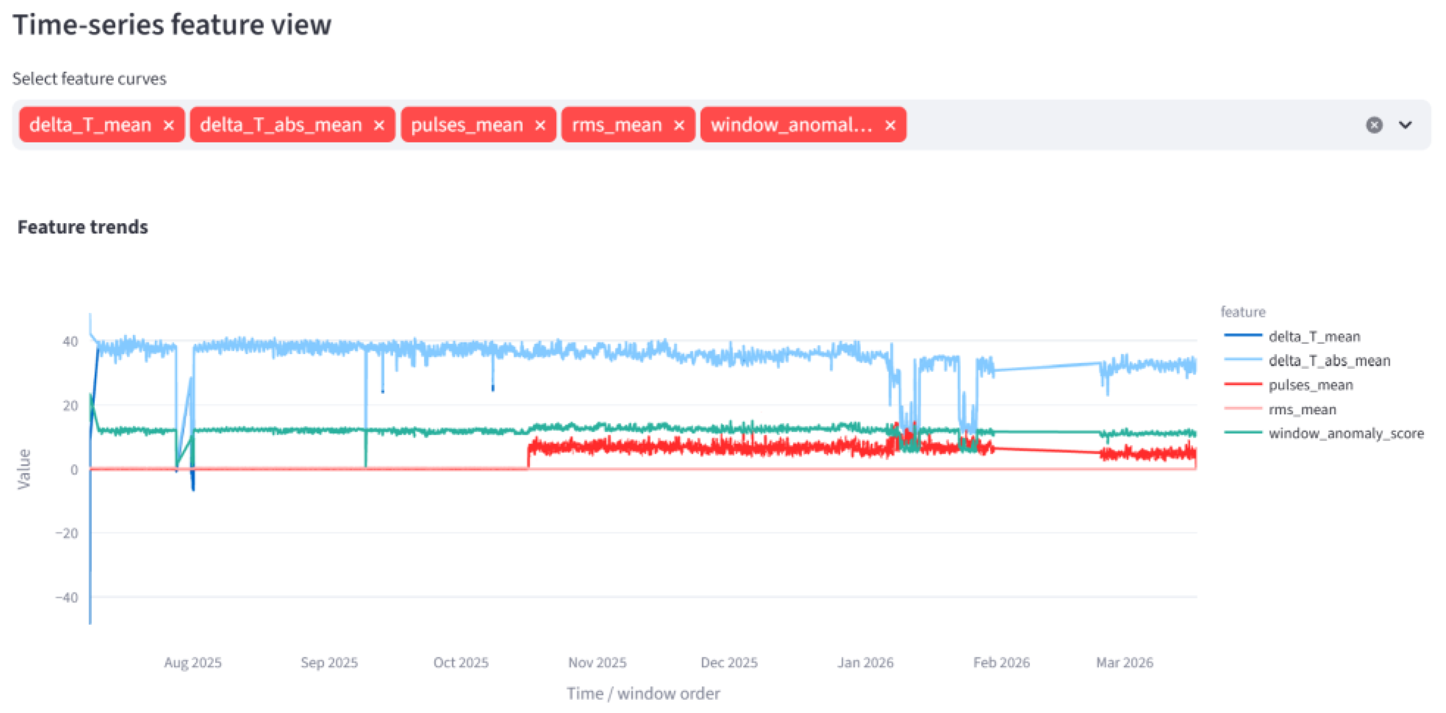
The time-series view provides the missing link between the numerical prediction and the underlying physical measurements. By displaying the selected features over time, the operator can inspect whether a predicted condition is accompanied by a persistent thermal or acoustic signature, a transition, or a cycling pattern. This is important for explainability: the dashboard does not claim to provide causal explanations, but it allows the user to inspect the sensor evidence associated with a prediction rather than treating the classifier as a black box.
Taken together, the three views demonstrate an end-to-end workflow from runtime data ingestion to fleet-level scope control, asset-level condition distribution and time-series inspection. The dashboard remains a prototype rather than a production maintenance platform: the thesis explicitly notes that it does not yet integrate live industrial streams, automated work orders or long-term operator feedback
Nevertheless, including the visualization layer is important because it shows how the ML output could be incorporated into an industrial decision-support workflow.
6.7. What the Results Demonstrate and What They Do Not
The results demonstrate that a multimodal, window-based feature representation can support high-performing six-state classification within a defined device scope. They also demonstrate that the selected HistGradientBoosting model remains strong under chronological evaluation and that a conservative routing mechanism can prevent unsupported records from being treated as formal predictions.
The results do not yet demonstrate universal steam-trap fault diagnosis. The labels are engineering-rule-based, the later time blocks do not contain all six states, and the device population is limited. These constraints are not secondary details; they define the scientific boundary of the result. The most defensible claim is therefore that the proposed workflow provides a promising and technically coherent condition-monitoring prototype for supported devices.
This distinction is particularly important when comparing the work with recent AI-based steam-trap studies. A 2025 study by Kim et al. used industrial data from aluminum and food-processing plants, combined sensor and contextual information, and reported independently supported fault labels together with an AI-based diagnostic workflow. It also reported average thermal-energy savings of 6.92% across the two sites [7]. The present work differs by focusing on energy-autonomous sensing and by explicitly studying leakage-reduced feature selection and scope-aware inference. The two approaches are therefore complementary rather than directly interchangeable.
7. Discussion
The conceptual transition from leak detection to condition monitoring is the central scientific step of this paper. The previous system established that thermoelectric harvesting, temperature measurement and ultrasound can provide a practical autonomous steam-trap monitoring node. The present work adds an interpretation layer capable of representing several operating states. This changes the role of the sensor from an alarm generator into a source of condition information.
A multi-state output can also support prioritization. If hundreds of traps are monitored, maintenance teams rarely have the resources to inspect every abnormal observation immediately. A failed-open indication can be prioritized according to estimated steam-loss impact, while a degraded or cycling indication can be accumulated as a trend. The value of the ML layer therefore comes from converting a large stream of heterogeneous observations into a manageable set of condition categories.
7.1. From Leak Detection to Condition Monitoring
The principal advance over the previous steam-trap IIoT work is the change in the information produced by the system. The earlier device demonstrated that thermoelectric energy harvesting, temperature and ultrasound can support autonomous steam-leak monitoring. The present work uses the same physical sensing foundation but introduces temporal feature engineering and supervised classification to produce a richer condition description.
This transition is significant for industrial maintenance. A binary alarm can identify a problem, but a multi-state condition indicator can support prioritization. A failed-open state is associated with direct steam loss and therefore energy and emissions impact. A failed-closed state can indicate condensate-management risk. Degraded and abnormal cycling states may provide earlier indications of developing problems. The model therefore becomes an interpretation layer between raw sensor measurements and maintenance workflow.
The connection between energy harvesting and machine learning is deeper than simply powering the electronics. Machine learning benefits from repeated observations because many industrial failures are temporal. A batteryless sensor powered by process heat can operate while the thermal gradient exists, and the resulting long-term data stream can capture operating cycles, gradual degradation and intermittent leakage.
This creates a feedback loop between hardware and analytics. Better energy harvesting enables more frequent measurements; richer measurements improve feature engineering; better features improve condition classification; and better classification can identify energy losses that justify maintaining the monitoring system. In this sense, the TEG is part of the information [2] architecture, not merely a replacement for a battery.
7.2. Why Thermoelectric Powering Matters to Machine Learning
The relationship between energy harvesting and machine learning is indirect but fundamental. Continuous monitoring requires a sustainable energy budget. If the sensor depends on a battery with a limited service interval, acquisition and communication frequency must be constrained or maintenance must periodically replace the energy source. A thermoelectric node instead uses the process heat that is already available at the installation point.
The autonomous power architecture consequently enables a sensing strategy based on repeated measurements over long periods. This temporal density is valuable for machine learning because cycling, degradation and intermittent leakage are dynamic phenomena. In this sense, energy harvesting is not merely a hardware optimisation; it enables the data-generation regime required by the condition-monitoring algorithm.
7.3. Industrial Scalability
Steam-trap monitoring is a distributed sensing problem. A large facility may require hundreds or thousands of nodes, making wiring and battery maintenance important lifecycle considerations. The combination of batteryless operation and LoRaWAN [14] is therefore aligned with large-scale deployment. The previous system demonstrated a data transmission interval of approximately five minutes in its steam-trap implementation, while the present ML workflow operates on window-level information rather than requiring continuous raw waveform transmission.
A scalable deployment should nevertheless account for thermal availability, radio coverage, installation variability, device heterogeneity and model scope. The scope-aware architecture is therefore a practical component of scalability rather than an optional software feature.
From Steam Loss to Avoided CO2
The environmental impact should ultimately be expressed using the physical loss avoided by maintenance. For a measured leakage mass flow m_dot and operating duration t, the annual lost steam mass is M_loss = m_dot t. The corresponding thermal loss depends on the enthalpy difference between the leaked steam and the water/steam that must be generated to replace it. A simplified energy estimate can therefore be written as:
E_loss ≈ M_loss (h_steam − h_makeup)/η_boiler (3)
where η_boiler represents the effective boiler efficiency.
Once the replacement fuel energy is known, avoided greenhouse-gas emissions can be estimated from the site-specific emission factor EF_fuel, giving m_CO2eq ≈ E_fuel × EF_fuel. This formulation makes clear why a universal CO2 number is inappropriate: steam pressure, feedwater temperature, boiler efficiency, operating hours and fuel type can change the result by a large factor.
The earlier work used a representative leakage rate of 0.5 kg/min to illustrate the scale of the problem and obtained approximately 262.8 tonnes of steam per year under continuous operation.
The present paper deliberately does not convert this example directly into a universal carbon saving. Instead, it proposes a plant-specific calculation as the appropriate next validation step.
A particularly valuable future KPI would be avoided kg CO2-eq per sensor-year, coupled to the number of confirmed and repaired failed traps. This would connect classification performance with the actual sustainability value of the monitoring system.
7.4. Environmental Impact
A site-specific environmental assessment can be derived from measured or estimated leakage mass flow. If m_dot_leak is the leakage rate, h_leak is the enthalpy of the leaked steam and h_makeup is the enthalpy associated with replacement water, the thermal loss rate can be approximated as:
Qloss = mdot_leak (hleak − hmakeup) (4)
Annual avoided thermal loss is then obtained from the operating time, while fuel and CO2 savings can be calculated from boiler efficiency and the applicable fuel emission factor. This approach is preferable to a universal CO2 factor because steam pressure, fuel, boiler efficiency and operating schedule vary between plants.
The environmental value of the proposed system has two components. The first is avoided process energy loss when failed or degraded steam traps are detected earlier. The second is the reduction in monitoring infrastructure burden associated with battery replacement and wiring. The magnitude of the first component depends strongly on steam pressure, trap geometry, operating hours, boiler efficiency and fuel mix; therefore, a site-specific carbon calculation should be used for industrial deployment.
For future validation, the most useful metric is not simply classification accuracy but avoided steam loss per detected and repaired trap. Combining measured leakage, intervention time and plant-specific emissions factors would allow the monitoring system to be evaluated directly in terms of kg CO2-eq avoided per sensor-year.
Table 9.
Model’s detections.
| Dimension | Previous steam-trap work | Present work | Scientific implication |
| Power | TEG-powered, batteryless node | Same autonomous energy concept | Enables continuous sensing without primary battery |
| Sensing | Temperature + ultrasound | Temperature + ultrasound + derived cycling features | Multimodal condition representation |
| Output | Leak detection / abnormality | Six-state condition categories | Richer maintenance information |
| Analytics | Rule/feature interpretation | Tree-based ML + leakage reduction | Nonlinear multimodal classification |
| Evaluation | Experimental device characterization | Chronological, robustness and scope-aware evaluation | Closer to deployment-oriented assessment |
| Validation | Demonstrated sensing; limited confirmed faults | Engineering-rule labels; independent validation still needed | Defines the current scientific boundary |
7.5. Limitations
Several limitations must be recognised. First, the labels used in the present dataset are rule-informed pseudo-labels and are not independently confirmed ground-truth failure records for every window. Second, the current-scope dataset represents a limited device and feature distribution and should not be generalised automatically to all steam-trap technologies. Third, later chronological blocks do not contain all six states, limiting the interpretation of temporal performance.
Fourth, although the model achieves high numerical performance, field validation under confirmed fault conditions remains necessary. Finally, the present work evaluates the ML pipeline primarily at the window level. Future studies should connect predictions to maintenance records, intervention outcomes and measured steam-loss reductions.
8. Deployment Roadmap and Future Experimental Validation
Moving from the current prototype [15] to a validated industrial monitoring system requires a staged validation Programme. The first stage should establish independent labels by combining the sensor predictions with maintenance records, expert inspection, controlled fault tests and, where possible, disassembly of suspect traps. The goal is to create a subset of windows for which the physical state is known independently of the rule-based labelling framework.
The second stage should expand the device population. The present classifier is explicitly limited to current-scope devices. New trap types, sensor revisions and installation configurations should be introduced through a qualification process rather than being merged directly into the production model. For each new population, feature distributions should be compared with the training population and the model should be re-evaluated before formal predictions are enabled.
The third stage should evaluate temporal drift over longer periods. The current 70/15/15 time-block experiment is useful but incomplete because later blocks do not contain all six classes. A longer field dataset should contain multiple operating cycles, seasonal conditions, maintenance interventions and periods of changing process load. This would allow drift metrics and performance degradation to be quantified explicitly.
The fourth stage should close the loop with maintenance outcomes. Each formal prediction should eventually be associated with an inspection or maintenance event. The system could then evaluate not only whether a window was classified correctly, but whether the alert led to an effective intervention and how much steam loss was avoided. This would move the evaluation from algorithmic accuracy toward operational value.
Finally, the runtime system should incorporate model versioning, feature-schema validation, missing-data detection, communication-quality monitoring and operator feedback. These mechanisms are consistent with the thesis future-work recommendations, which identify field-confirmed inspections, longer monitoring periods, unseen-device tests, feature-ablation studies and live deployment controls as the next steps [9].
The principal conclusion is that thermoelectric energy harvesting, multimodal sensing and machine learning can be combined into a coherent architecture for autonomous steam-trap condition monitoring. The TEG supplies the energy required by the sensing and communication node; temperature and ultrasonic measurements provide complementary physical evidence; window-level feature engineering converts these signals into a structured representation; and machine learning transforms the representation into six condition categories. The runtime dashboard further demonstrates how the resulting condition states can be exposed to users together with scope and sensor context.
The selected Histogram-based Gradient Boosting model achieved 0.9853 test accuracy and 0.8822 test macro-F1 under the non-strict leakage-reduced chronological evaluation, outperforming Random Forest and Extra Trees in the current dataset. The robustness experiment demonstrated, however, that aggressive removal of potentially rule-related features reduces macro-F1 substantially. This result motivates further work on physically grounded features and independently verified labels.
The scope-aware runtime architecture is equally important. Only supported current-scope records receive formal predictions, while legacy records are retained for shadow analysis and out-of-scope records are rejected. This explicit boundary is essential for industrial AI, where unsupported predictions can be more damaging than an explicit ‘not qualified’ state. Taken together, the work demonstrates a pathway from process waste heat to actionable industrial information. The next scientific step is not simply to increase classifier complexity, but to validate the six-state taxonomy against independent field evidence, expand the device population, quantify avoided steam loss and CO2 emissions, and demonstrate long-term deployment stability.
9. Conclusions
This paper presented an autonomous steam-trap condition-monitoring architecture combining thermoelectric energy harvesting, multimodal sensing, LoRaWAN IIoT communication and machine learning. The system builds on a previously demonstrated heat-powered steam-leak sensor and extends its analytical capability from binary leak detection to six-state condition monitoring.
The machine-learning study used 6,354 current-scope windows and 117 candidate features derived from temperature, ultrasonic, cycling and statistical information. Random Forest, Extra Trees and Histogram-based Gradient Boosting were compared using a leakage-reduced feature configuration. Histogram-based Gradient Boosting provided the best balance of validation and chronological test performance, achieving 0.9958 validation accuracy and 0.9550 validation macro-F1, followed by 0.9853 test accuracy and 0.8822 test macro-F1.
The temporal evaluation and scope-aware routing are particularly relevant to industrial deployment. The model remained effective on later chronological data, while the runtime architecture avoided issuing formal predictions for unsupported devices. These design choices are important because a reliable industrial AI system must provide not only high accuracy but also an explicit boundary for when its predictions are valid.
The proposed approach demonstrates a path from waste heat to actionable condition information: thermal energy powers the sensor, multimodal measurements capture physical behaviour, wireless IIoT infrastructure delivers the data, and machine learning transforms the data into a condition state. Future work should focus on independently confirmed fault labels, larger cross-device datasets, field validation under controlled failures, explainable feature analysis and direct quantification of avoided steam loss and CO2 emissions.
Author Contributions
Conceptualization, R.A., and L.K.; methodology, R.A.; software and machine-learning development, L.K.; investigation, R.A., R.M. and L.K.; data curation, L.K.; writing—original draft preparation, R.A.; writing—review and editing, R.A., R.M. and L.K.; supervision, R.A.; project administration, R.A. All authors have read and agreed to the published version of the manuscript.
Funding
This research received no external funding.
Data Availability Statement
The industrial steam-trap monitoring data used in this study were provided by Alternative Energy Innovations S.L. (AEInnova). The raw datasets (DatasetI and DatasetZ) are not publicly available due to confidentiality restrictions associated with the industrial data. The implementation code, trained-model package, scope-routing configuration, post-processing rules, and dashboard prototype are publicly available in the project GitHub repository at https://github.com/1822971148-ux/steam-trap-predictive-maintenance. The public repository does not contain the confidential raw industrial datasets.
Acknowledgments
The authors would like to thank the operators and technical staff at the pharma plant for their collaboration and for providing access to the facilities and equipment required to conduct the experimental trials during the first quarter of 2026. During the preparation of this manuscript, the authors used ChatGPT (GPT-5.6 Luna, OpenAI) as a writing and language-support tool to improve the clarity, readability, and structure of the manuscript. The tool was not used to generate or analyze experimental data, nor to draw scientific conclusions. The authors have reviewed and edited the output and take full responsibility for the content of this publication.
Conflicts of Interest
The authors declare no conflicts of interest.
References
- Einstein, D.; Worrell, E.; Khrushch, M. Steam Systems in Industry: Energy Use and Energy Efficiency Improvement Potentials; Lawrence Berkeley National Laboratory, 2001. [Google Scholar]
- Sarco, Spirax. Steam Traps and Their Failures. Technical resource. [CrossRef]
- Armstrong International. SteamEye: Steam Trap Testing and Monitoring. Technical resource.
- U.S. Department of Energy. Steam System Survey Guide. In Industrial Technologies Program.
- Aragonés, R.; Oliver, J.; Ferrer, C. Thermoelectric Generator-Powered Long-Range Wireless Real-Time Steam Leak Detection in Steam Traps. Future Internet 2024, 16, 474. [Google Scholar] [CrossRef]
- Aragonés, R.; Oliver, J.; Malet, R.; Oliver-Parera, M.; Ferrer, C. Model and Implementation of a Novel Heat-Powered Battery-Less IIoT Architecture for Predictive Industrial Maintenance. Information 2024, 15, 330. [Google Scholar] [CrossRef]
- Kim, C.; Cho, K.; Joe, I. Artificial Intelligence-Based Fault Diagnosis for Steam Traps Using Statistical Time Series Features and a Transformer Encoder-Decoder Model. Electronics 2025, 14, 1010. [Google Scholar] [CrossRef]
- Li, S.; Zhao, Q.; Liu, J.; Zhang, X.; Hou, J. Noise Reduction of Steam Trap Based on SSA-VMD Improved Wavelet Threshold Function. Sensors 2025, 25, 1573. [Google Scholar] [CrossRef]
- Kong, L. A Scope-Aware Six-State Condition Monitoring System for Steam Traps Using Machine Learning. Master Thesis, MSc in Research and Innovation for Computer-based Science and Engineering, 2026. [Google Scholar]
- Breiman, L. Random Forests. Mach. Learn. 2001, 45, 5–32. [Google Scholar] [CrossRef]
- Geurts, P.; Ernst, D.; Wehenkel, L. Extremely Randomized Trees. Mach. Learn. 2006, 63, 3–42. [Google Scholar] [CrossRef]
- Friedman, J.H. Greedy Function Approximation: A Gradient Boosting Machine. Ann. Stat. 2001, 29, 1189–1232. [Google Scholar] [CrossRef]
- Pedregosa, F.; Varoquaux, G.; Gramfort, A.; et al. Scikit-learn: Machine Learning in Python. J. Mach. Learn. Res. 2011, 12, 2825–2830. [Google Scholar]
- Mekki, K.; Bajic, E.; Chaxel, F.; Meyer, F. A Comparative Study of LPWAN Technologies for Large-Scale IoT Deployment. ICT Express, 2019. [Google Scholar]
- Aragonés, R.; Oliver, J.; Ferrer, C. Enhanced Heat-Powered Batteryless IIoT Architecture with NB-IoT for Predictive Maintenance in the Oil and Gas Industry. Sensors 2025, 25, 2590. [Google Scholar] [CrossRef]
Figure 1.
Steam circuit composed by the boiler, steam pipeline and steam trap.
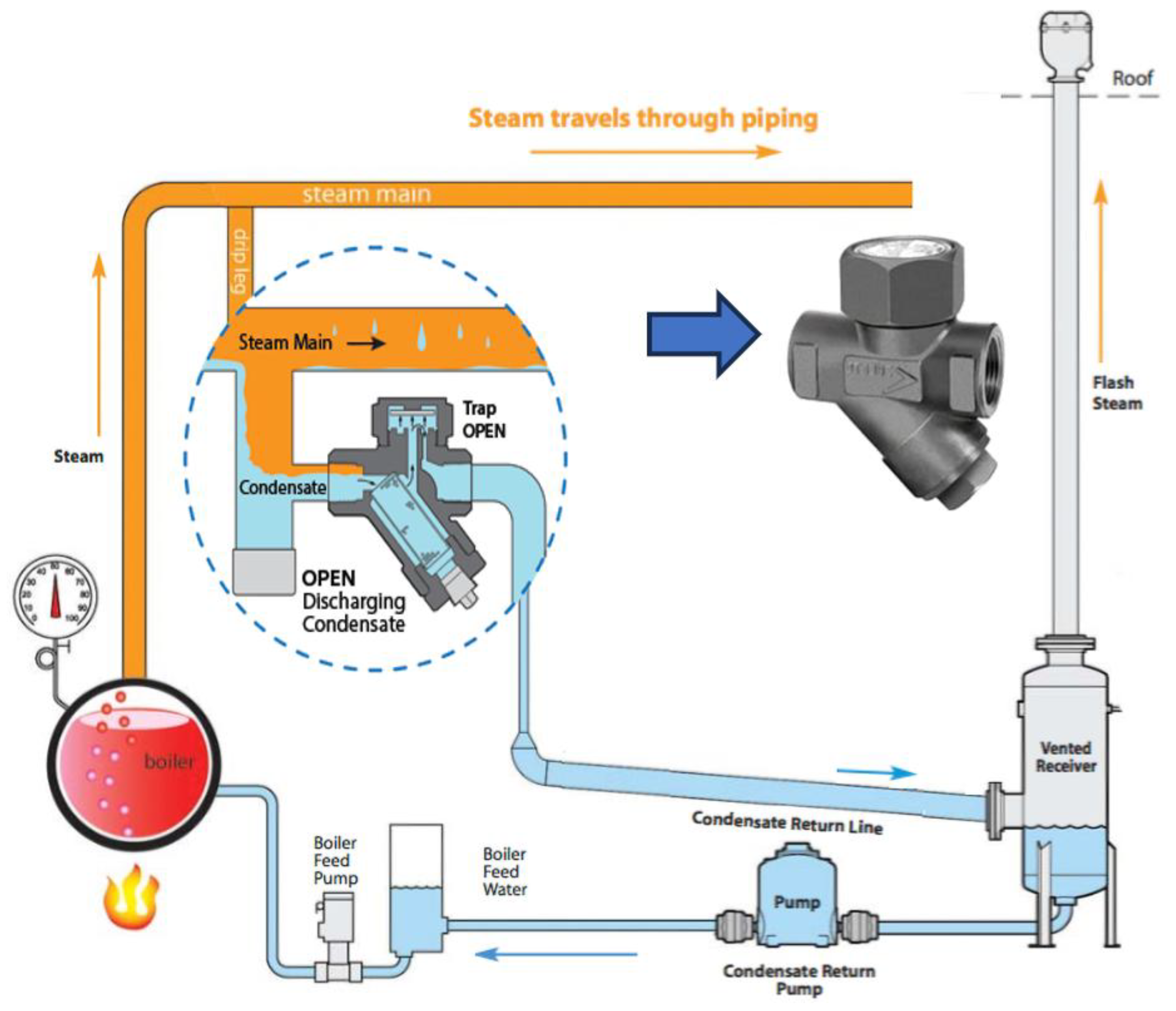
Figure 2.
Autonomous iIoT architecture for steam traps condition monitoring.
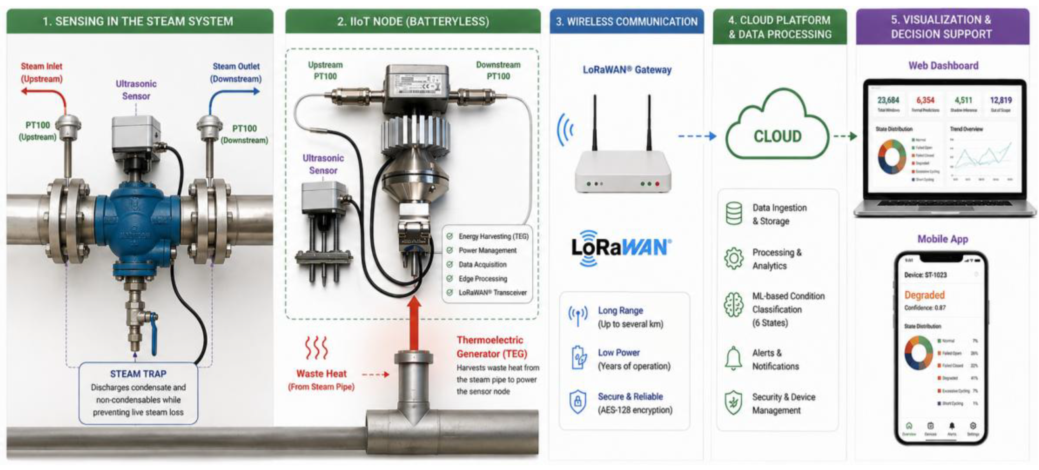
Figure 3.
Thermoelectric module characterization.
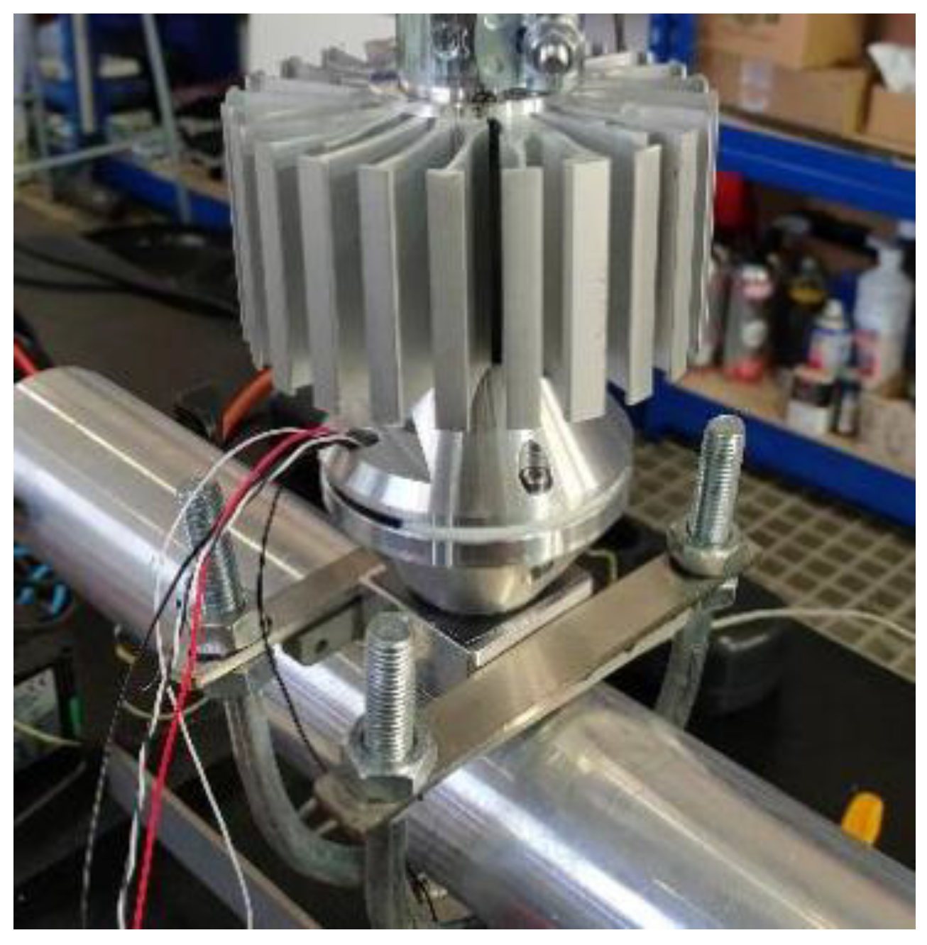
Figure 4.
(a). Generated electrical power of the thermoelectric generator as a function of hot-side surface temperature for the ambient temperatures reported in the previous study. Data reproduced from the original experimental dataset. (b). Open-circuit voltage of the thermoelectric generator as a function of hot-side surface temperature for the ambient temperatures reported in the previous study. Data reproduced from the original experimental dataset.
Figure 4.
(a). Generated electrical power of the thermoelectric generator as a function of hot-side surface temperature for the ambient temperatures reported in the previous study. Data reproduced from the original experimental dataset. (b). Open-circuit voltage of the thermoelectric generator as a function of hot-side surface temperature for the ambient temperatures reported in the previous study. Data reproduced from the original experimental dataset.
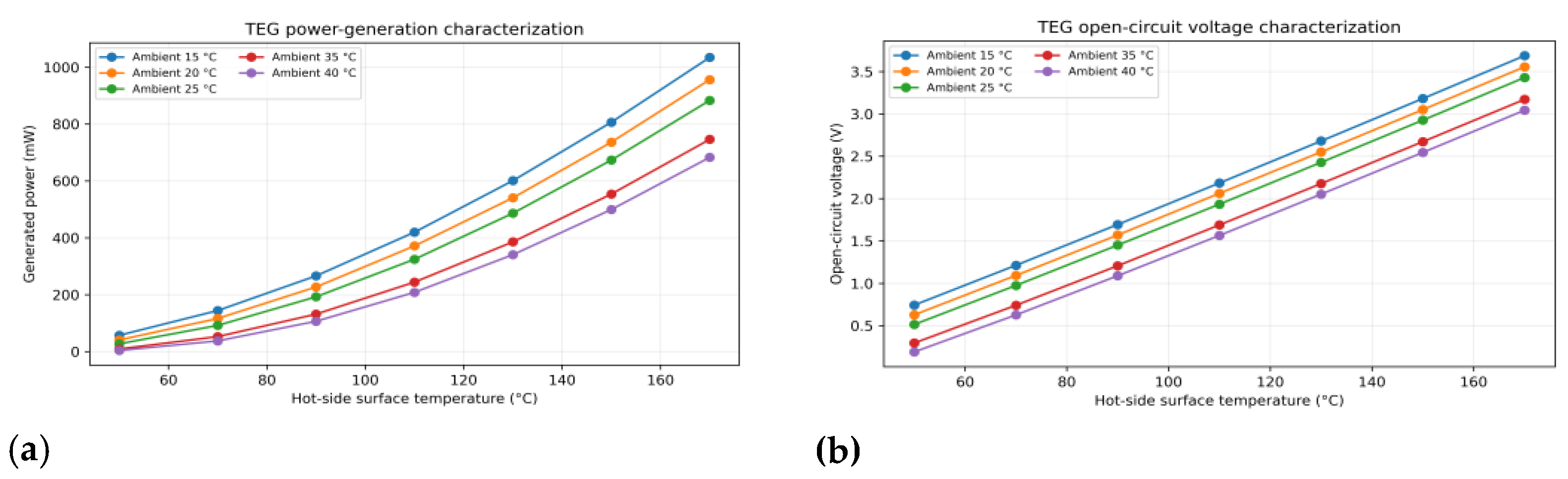
Figure 5.
System implementation in a pharma facility on a mechanical steam trap.
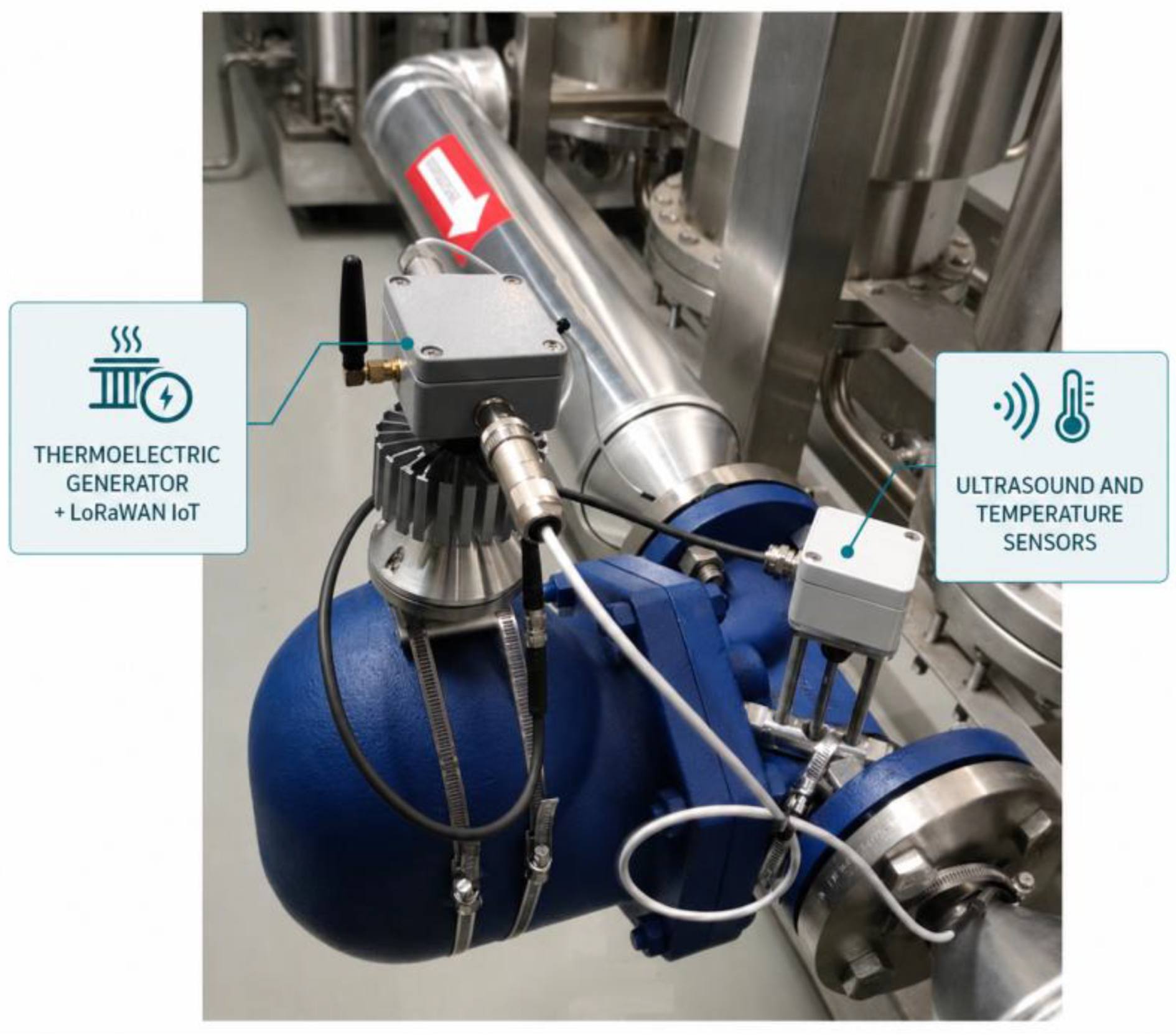
Figure 6.
Validation and test macro-F1 for the three candidate classifiers under the non-strict leakage-reduced configuration.
Figure 6.
Validation and test macro-F1 for the three candidate classifiers under the non-strict leakage-reduced configuration.
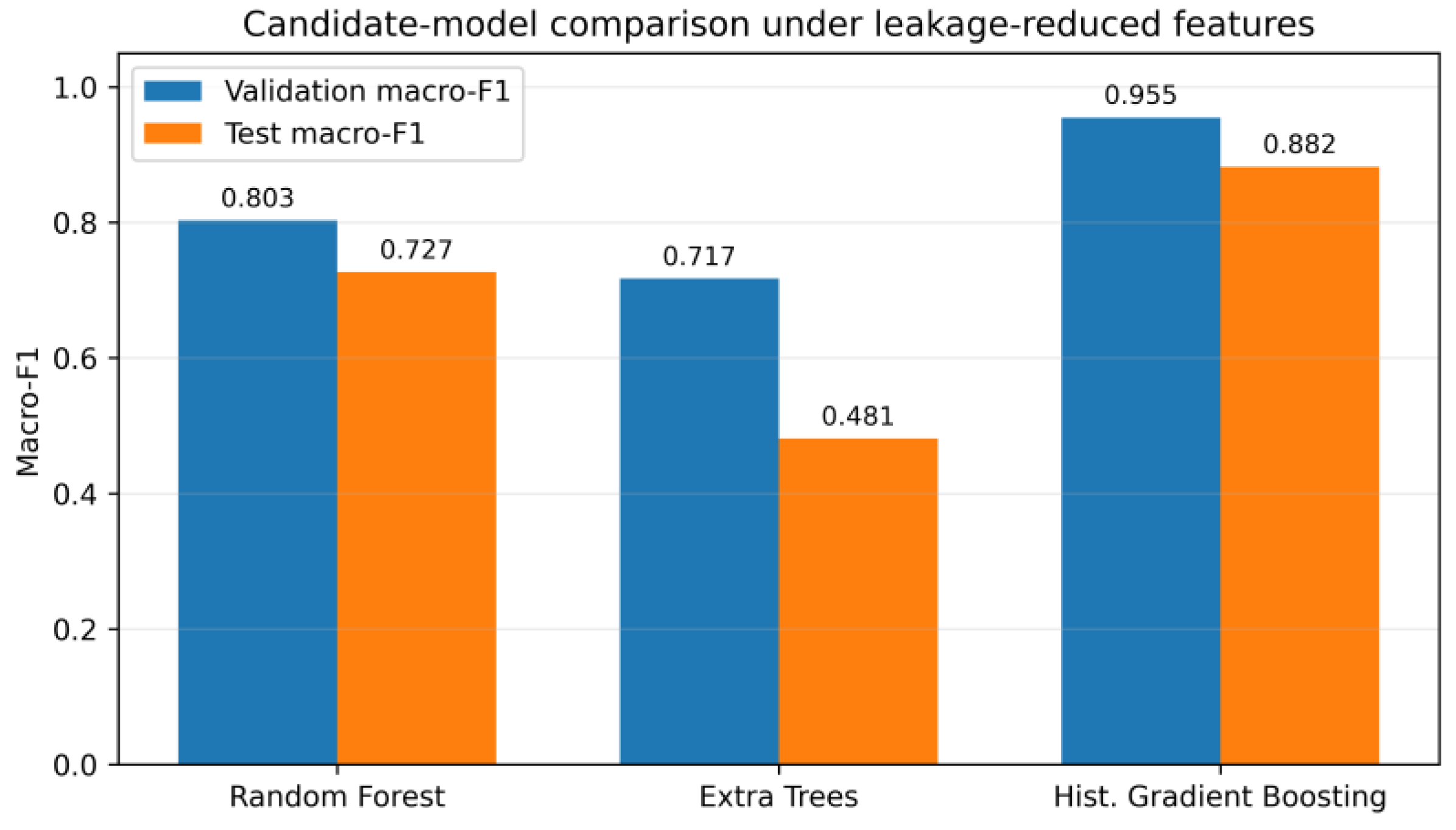
Figure 7.
Accuracy and macro-F1 across the chronological training, validation and test blocks for the selected Histogram-based Gradient Boosting model.
Figure 7.
Accuracy and macro-F1 across the chronological training, validation and test blocks for the selected Histogram-based Gradient Boosting model.
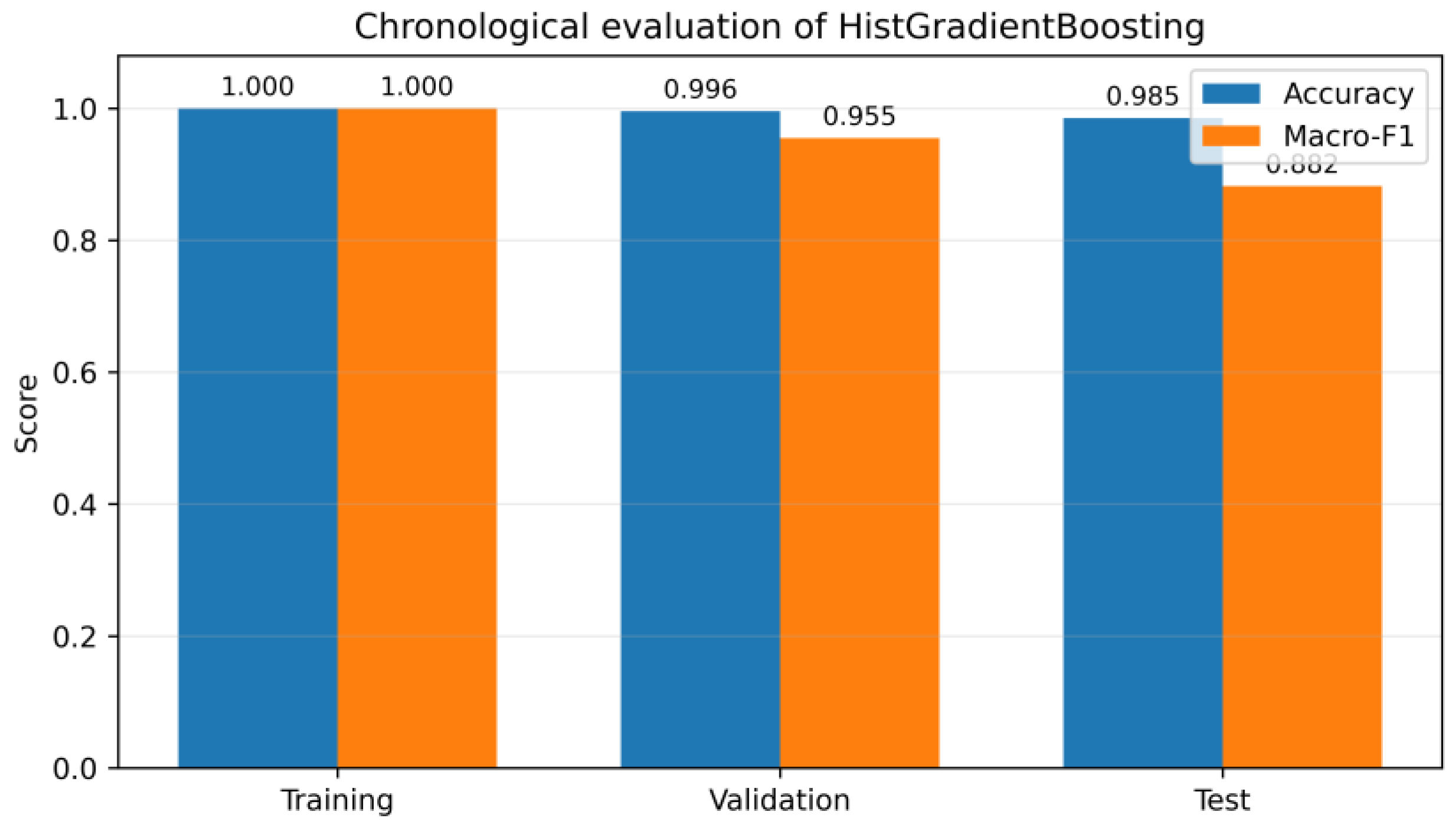
Figure 8.
Validation and test macro-F1 under non-strict and strict leakage-reduced feature selection.
Figure 8.
Validation and test macro-F1 under non-strict and strict leakage-reduced feature selection.
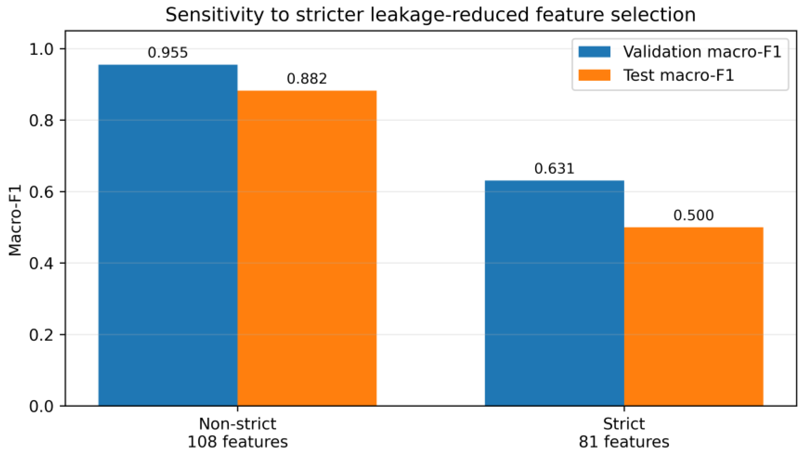
Figure 9.
Runtime distribution of current-scope, legacy/shadow and out-of-scope records.
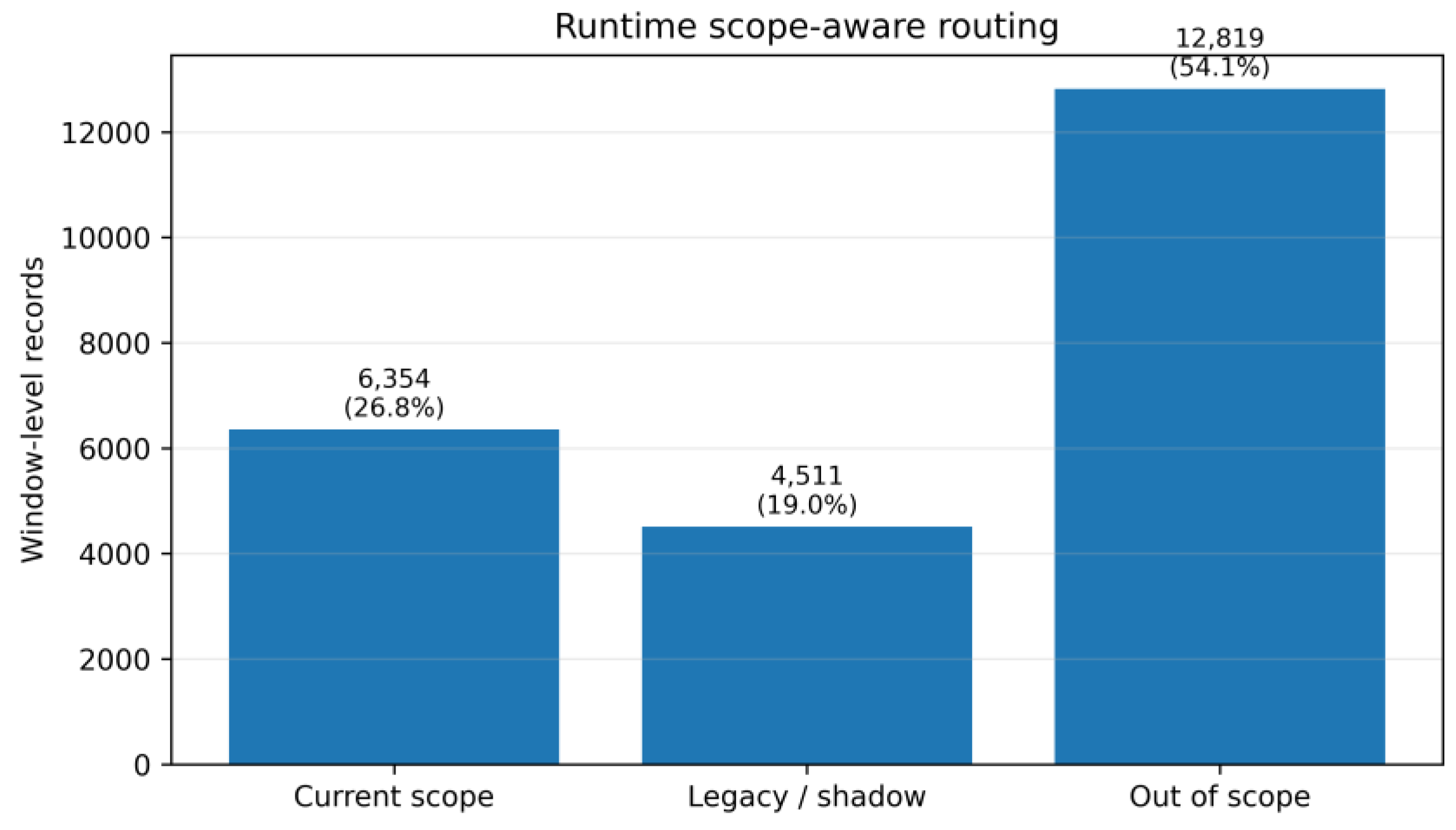
Figure 11.
Prototype dashboard overview showing the runtime data source, system summary and scope-aware record counts. The dashboard processes the runtime output generated by the monitoring pipeline [4].
Figure 11.
Prototype dashboard overview showing the runtime data source, system summary and scope-aware record counts. The dashboard processes the runtime output generated by the monitoring pipeline [4].
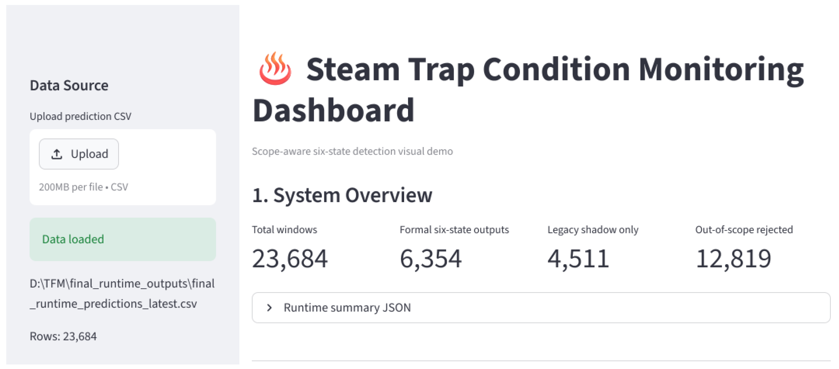
Figure 12.
Device Explorer view for a selected device, showing the number of available windows, model/scope status, mean confidence and the distribution of predicted condition states [4].
Figure 12.
Device Explorer view for a selected device, showing the number of available windows, model/scope status, mean confidence and the distribution of predicted condition states [4].
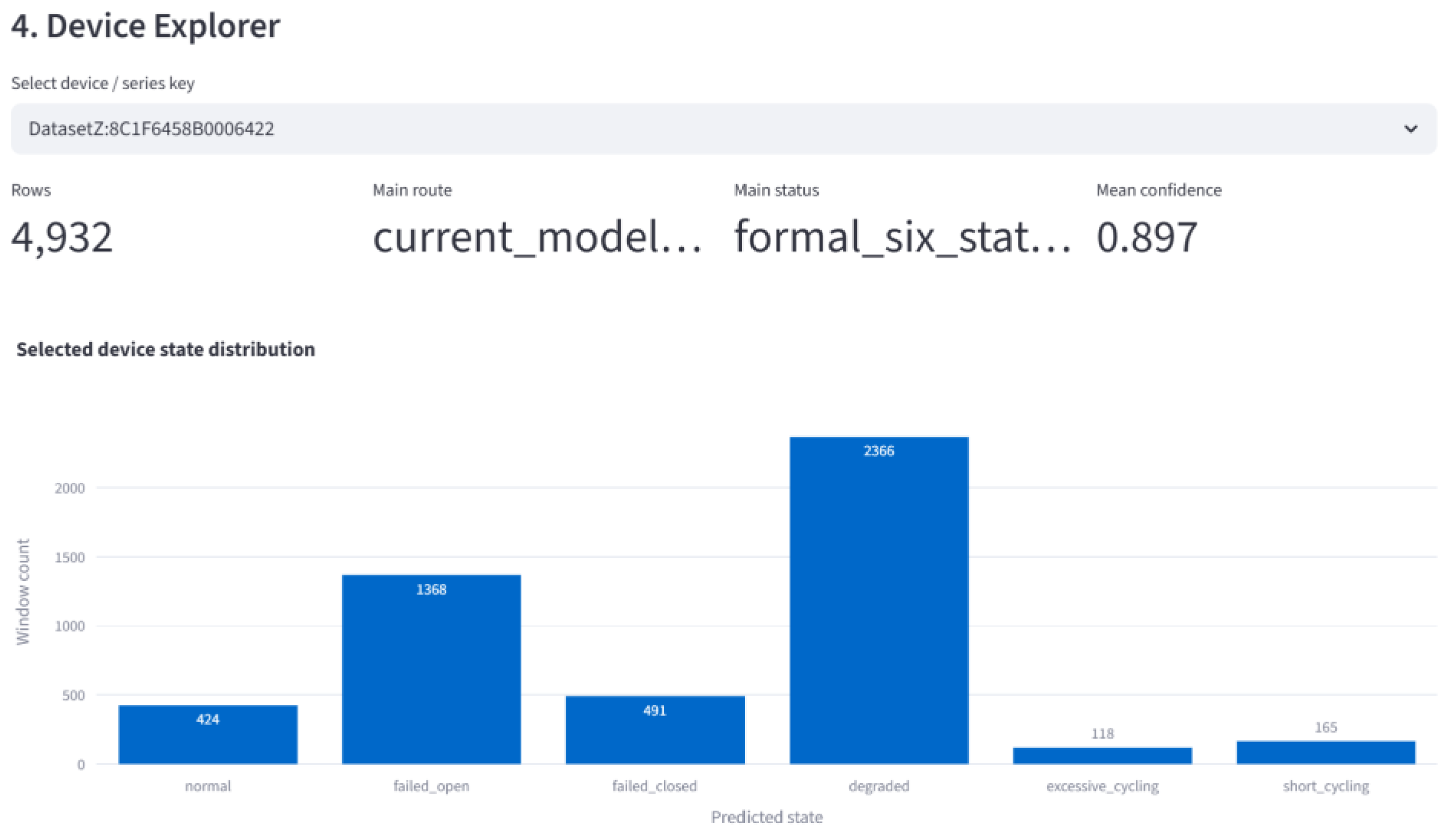
Table 1.
Steam trap family.
| Trap family | Dominant physical mechanism | Monitoring implications |
|---|---|---|
| Mechanical | Density / condensate level | Temperature and continuous or semi-continuous discharge patterns are relevant |
| Thermodynamic | Flow/pressure dynamics | Pulse, cycle and ultrasonic behaviour are particularly informative |
| Thermostatic | Temperature response | Inlet/outlet temperature difference and thermal transients are important |
Table 3.
Thermoelectric performance.
| Condition | Hot-side T | Ambient T | Reported result |
| Maximum open-circuit voltage | 170 °C | 15 °C | 3.687 V |
| Maximum generated power | 170 °C | 15 °C | 1.034 W |
| Characterization range | 50–170 °C | 15–40 °C | 5 ambient conditions |
| Temperature step | 10 °C | — | 20 min stabilization/step |
Table 6.
Process’ results.
| Period | Accuracy | Macro-F1 | Interpretation |
|---|---|---|---|
| Training | 1.0000 | 1.0000 | Fit to training data |
| Validation | 0.9958 | 0.9550 | Model-selection period |
| Final chronological test | 0.9853 | 0.8822 | Later unseen period |
Disclaimer/Publisher’s Note: The statements, opinions and data contained in all publications are solely those of the individual author(s) and contributor(s) and not of MDPI and/or the editor(s). MDPI and/or the editor(s) disclaim responsibility for any injury to people or property resulting from any ideas, methods, instructions or products referred to in the content. |
© 2026 by the authors. Licensee MDPI, Basel, Switzerland. This article is an open access article distributed under the terms and conditions of the Creative Commons Attribution (CC BY) license (http://creativecommons.org/licenses/by/4.0/).
Copyright: This open access article is published under a Creative Commons CC BY 4.0 license, which permit the free download, distribution, and reuse, provided that the author and preprint are cited in any reuse.