

Submitted:
01 September 2026
Posted:
02 September 2026
You are already at the latest version
Abstract
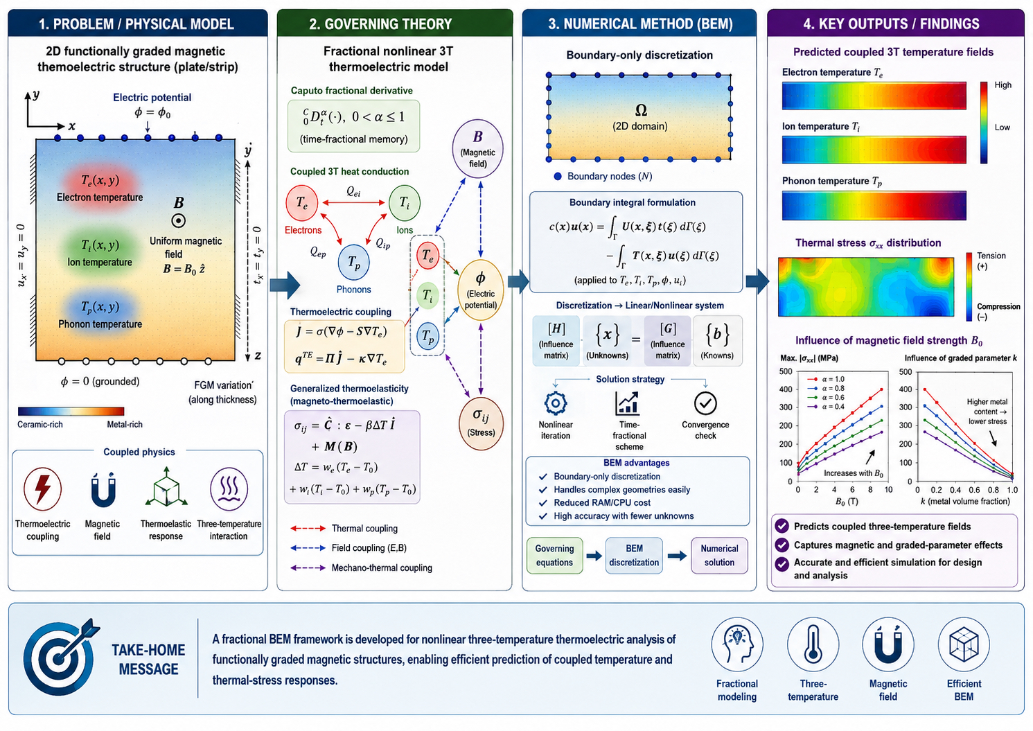
This study develops a fractional boundary element framework for the numerical analysis of nonlinear three temperature behavior in functionally graded magnetic thermoelectric materials. The formulation incorporates the coupled interactions among electron, ion, and phonon temperature fields together with magnetic, electric, and mechanical effects. A boundary element discretization is combined with fractional time modeling to provide an efficient computational strategy for problems involving complex geometries and strongly coupled material behavior. The proposed approach reduces the need for extensive domain discretization and therefore offers advantages in computational storage and solution efficiency. Numerical investigations demonstrate that the fractional order and material gradation significantly influence the magnitude and spatial distribution of thermal stresses. The computed results are also compared with established numerical approaches for representative limiting cases, showing close agreement and supporting the reliability of the proposed formulation. The developed methodology provides an effective computational tool for investigating coupled thermal, electromagnetic, and mechanical responses in advanced functionally graded thermoelectric structures.
Keywords:
fractional-order thermoelasticity
; three-temperature model
; boundary element method
; functionally graded materials
; magneto-thermoelectric coupling
; nonlinear heat conduction
; thermal stress
; CA-GMRES
1. Introduction
Thermal transport in solids is closely linked to lattice vibrations. Initial descriptions of quantum mechanics that were developed for electromagnetic radiation and heat capacity of solids formed the framework for the study of quantized vibrational energies of crystals. These lattice vibrations, which are typically modeled by phonons, transport thermal and acoustic energies in solids and thus constitute an essential aspect of their thermal and mechanical response. This is particularly significant in multi-field materials, where the performance is contingent upon thermal, electrical, magnetic, and elastic interactions.
Many materials exhibit pronounced changes in their effective properties when subjected to electric or magnetic fields. This behavior has motivated the development of electrorheological and magnetically responsive fluids, electro-active elastomers, and magneto-active elastomers for applications such as actuators, clutches, shock absorbers, valves, and adaptive devices. In solids, the coupling between field-induced changes in microstructure and the resulting elastic response provides a useful mechanism for designing multifunctional materials with controllable stiffness and compliance.
Fractional calculus (FC) extends differentiation and integration to non-integer orders and has become a useful modeling framework for systems with memory and hereditary effects [4]. Fractional formulations have been applied to circuit design [5], vibration analysis [7], hydro-turbine dynamics [8], control engineering [9,10], nanotechnology [11], and biological processes [12,13]. Fractional adaptive algorithms have also been developed for parameter estimation [1,2,3,14,15,16], where the fractional order can influence convergence and estimation behavior. These developments motivate the use of fractional operators in coupled thermomechanical models whose transient response cannot be represented adequately by classical integer-order descriptions.
The foundations of magnetoelasticity were established by Knopoff [17], Chadwick [18], and Kaliski and Petykiewicz [19]. With the growth of high-performance computing, numerical simulation has become an increasingly important complement to magnetic experiments, particularly when direct testing is difficult, hazardous, or expensive. Accurate computational models are therefore essential for resolving coupled magnetic, thermal, and mechanical fields in advanced materials.
The interaction of magnetic, thermal, and deformation fields in thermoelastic solids is relevant to geophysics, plasma physics, and multifunctional material systems. In many formulations, the magnetic field enters the mechanical equations through Lorentz forces and the electrical response through a modified Ohm law. Generalized thermoelastic models extend classical heat conduction by incorporating relaxation and non-Fourier effects. Ezzat and Awad developed a micropolar generalized magneto-thermoelastic model based on modified Ohm and Fourier laws. Three-temperature theories have subsequently been investigated for micropolar thermoelasticity [21], carbon-nanotube-reinforced composites [22], micropolar piezothermoelasticity [23], micropolar magneto-thermoviscoelasticity [24], and magneto-thermoviscoelasticity [25]. The strong nonlinearity and fractional character of these coupled models generally preclude closed-form solutions, making robust numerical techniques essential.
The present study constitutes a comprehensive re-examination, reconstruction, and substantive extension of earlier work undertaken within the same research program. The theoretical formulation, analytical assumptions, computational procedures, interpretation of results, and overall presentation have been systematically reassessed and, where necessary, reformulated to establish a more general, internally consistent, and methodologically rigorous framework. Particular attention has been devoted to identifying and resolving technical inaccuracies, methodological inconsistencies, and interpretive limitations present in the earlier work. All revisions, corrections, and substantive modifications presented in the current article were undertaken solely by the author of this work. Importantly, the formulation developed herein is broader in scope than the earlier collaborative analysis, which may be recovered as a restricted special case of the present framework when the corresponding simplifying assumptions, parameter restrictions, and constitutive conditions are imposed. The current contribution therefore extends beyond a conventional correction or incremental refinement and instead provides a comprehensive theoretical and computational framework within which the previous formulation is naturally embedded as a limiting case. Its principal objective is to correct and strengthen the scientific record, improve methodological reliability and transparency, and provide a more general basis for the analysis of the class of problems considered. In this respect, the present work reflects the author's commitment to the accuracy, integrity, completeness, and continuing improvement of the scientific record.
This work develops a fractional-order formulation for functionally graded magnetic thermoelectric materials within a nonlinear three-temperature generalized thermoelastic framework. The principal numerical contribution is a boundary element treatment of the coupled governing equations. By reducing the spatial discretization burden on the domain and retaining the geometric flexibility of BEM, the formulation is well suited to complex functionally graded structures. The numerical study focuses on the influence of the fractional-order parameter and the functional grading parameter on the thermal-stress field and evaluates the proposed implementation through special-case comparisons with previously reported GFDM and FEM–NMM results.
2. Formulation of the Problem
Consider the two-dimensional functionally graded magnetic thermoelectric structure shown in Figure 1, with thickness and length in a Cartesian coordinate system. The structure is subjected to an electric potential and placed in a constant external magnetic field. The material occupies a region bounded by , whose boundary subsets are defined according to the prescribed thermal and mechanical conditions.
The governing equations for fractional order three-temperature nonlinear generalized thermoelastic problems of functionally graded magnetic thermoelectric materials can be written as [26]
where
The fractional order three-temperature radiative heat conduction equations coupled with electron, ion and phonon temperatures can be expressed as
where
in which
and
| , | , | , |
The total energy of a unit mass can be described as follows:
Initial and boundary conditions can be written as
3. BEM Simulation for Temperature Field
The boundary element method is used in this section to solve the nonlinear time-dependent two dimensions three temperature (2D-3T) radiation diffusion equations that are coupled by electron, ion, and photon temperatures.
Caputo's integral definition and Grunwald-Letnikov integral definition are consistent with the Riemann-Liouville integral definition. Also, Caputo's derivative definition and Grunwald-Letnikov derivative definition are consistent with the Riemann-Liouville derivative definition. When the Riemann-Liouville or Grunwald-Letnikov definitions are compared to the Caputo definition, the functions that are derivable in the Caputo sense are significantly fewer. According to finite difference scheme of Caputo at times and , we obtain [27]
where
Based on equation (10), the fractional order heat equations (5) can be replaced by the following system
Based on the fundamental solution of (12), the direct formulation of boundary integral equation corresponding to (5) can be expressed as
which can be written in the absence of internal heat sources as follows
We assume that the time derivative of temperature can be approximated by a series of known functions in order to transform the domain integral in (14) to the boundary. and unknown coefficients as
Also, we assume that is a solution of
Thus, equation (14) results in the following boundary integral equation
where
And
In which the entries of are the coefficients of with matrix defined as [24]
Using the standard boundary element discretization scheme for equation (17) and using equation (19), we obtain the following set of ordinary differential equations
where matrices and are depending on the current time step, boundary geometry and material properties, and are, respectively, temperature and heat flux vectors at boundary nodes, and b is the internal heat generation vector
The diffusion matrix can be defined as
With
In order to solve equation (21) numerically the functions and are interpolated as
where the parameter determines the practical time in the present time step.
By differentiating equation (25) with respect to time we get
By substituting from Equations (25) - (27) into Equation (21), we obtain
By using initial and boundary conditions at and considering the previous time step solution as initial values for the next step, we obtain the following linear algebraic system
where is unknown matrix, and and are known matrices
4. BEM Simulation for Displacement and Microrotation Fields
Using the weighted residual method, the governing Equations (1) and (2) can be transformed into the following integral equations
in which
The boundary conditions are
The integration of the first term of equations (33) and (34) leads to
According to Huang and Liang [28], the boundary integral equation can be written as
The integration of (35)'s left-hand side by parts results in
According to Eringen [29], the elastic stress can be written as
Hence, equation (36) may be expressed as
Upon using the integration by parts once more to the left-hand side of (38), we obtain
where
According to Dragos [30], the fundamental solution may be written as
The weighting functions for and may be expressed as follows:
On the basis of Dragos [30], the fundamental solution may be expressed as
Using the above two sets of weighting functions into (39) we have
Thus, we obtain
in which
Now, we introduce the following relations
By discretizing the boundary, we can write (46) as
Which can be expressed as
By employing the following formula
Hence, equation (50) may be expressed as
The global matrix system equation for all nodes can be written as follows
where denotes the displacements and denotes the tractions.
Now, we can write (53) into the following form
The coupled systems of algebraic equations are coded into MATLAB (R2018a) using an explicit staggered predictor-corrector scheme. During each time step, the obtained linear systems of equations are solved by the communication-avoiding generalized minimal residual (CA-GMRES) approach in order to determine the temperature, displacement, and microrotation fields.
5. Numerical Results and Discussion
The numerical study examines the sensitivity of the three stress components in response to the variations of the fractional-order and functional grading parameters and . Furthermore, the performance features and the correctness of the model under particular conditions are studied. The BEM discretization is carried out by employing 42 boundary elements and 68 internal nodes, which are depicted in Figure 2. The following analysis will be made based on the trends observed on the considered x coordinate.
The effects of the fractional-order parameter for are depicted in Figure 3, Figure 4 and Figure 5. As seen from Figure 3, stays slightly compressive in most part of the domain and then starts decreasing very fast near the coordinate value approximately equal to 1.9 until recovering to the coordinate value of 2. Increase of leads to more negative values of , especially in the high-gradient zone.
For (Figure 4), the stress decreases with increasing and approaches zero near . At a fixed position, a larger produces a larger positive over most of the plotted interval. The separation between the curves is most pronounced away from the right boundary and narrows as the stress approaches its terminal value.
The response in Figure 5 is compressive and increases toward zero as increases. In contrast to , increasing moves downward, i.e., toward larger compressive magnitude. The fractional-order parameter therefore affects the individual stress components differently rather than producing a uniform amplification or attenuation of the entire stress tensor.
Figure 6, Figure 7 and Figure 8 study the effect of the functional grading coefficient . As can be seen in Figure 6, rises with an increase in , achieves its local maximum for , and falls off toward the right edge of the figure. An increase in not only enhances but also amplifies the value of the local maximum.
As can be seen from Figure 7, is a negative quantity over the plotted interval and tends to zero when → 2. Increasing makes more negative over most of the interval, while the three curves converge near the right boundary. The grading effect is therefore strongest in the interior and weakens close to the terminal boundary.
A similar grading sensitivity is observed for in Figure 8. Stress is still compressive but gets less and less negative as is increasing; on the other hand, the bigger is, the more negative value will be for a particular point. Contrary to , there is no confusion in distinguishing between the curves of
.
When put together, Figure 3, Figure 4, Figure 5, Figure 6, Figure 7 and Figure 8 illustrate the dependence of the thermoelastic deformation on the material property involved. An increase in reduces and and increases , whereas an increase in increases and reduces and . This shows that the memory effect and spatial variation of the material can serve different means of rearranging the thermal stress components.
Table 1 summarizes the reported computational-resource comparison for the present BEM implementation and the GFDM and FEM–NMM data used in the manuscript. The BEM calculation uses 68 nodes and 42 boundary elements, compared with 50,000 nodes and 20,000 elements for GFDM and 48,000 nodes and 18,000 elements for FEM–NMM. The reported CPU-time, memory, and disk-space metrics are also markedly smaller for BEM. These values are consistent with the principal computational advantage of a boundary-focused discretization. Because the table does not specify hardware, physical units, or normalization for the resource and accuracy metrics, the numerical values should be interpreted as implementation-specific reported metrics rather than hardware-independent performance benchmarks.
No independent published solution is available in the manuscript for the complete coupled fractional three-temperature problem; therefore, numerical consistency is examined through limiting cases that can be compared with the reported GFDM and FEM–NMM data. Figure 9 compares for and , corresponding to a homogeneous case, while Figure 10 considers and . In both comparisons, the BEM curve closely follows the reference curves over the full -range, including the steep stress-gradient region near . The visible deviations remain small relative to the overall stress variation. These special-case comparisons support the numerical consistency of the proposed BEM formulation, while the full coupled model would still benefit from additional independent benchmark or experimental validation.
6. Conclusions
This work presented a fractional boundary element formulation for nonlinear three temperature analysis of functionally graded magnetic thermoelectric materials. The proposed model integrates coupled thermal, electromagnetic, and mechanical effects within a unified computational framework and provides a practical approach for treating complex material behavior without requiring complete discretization of the interior domain.
The numerical results demonstrate that both the fractional order and the material gradation strongly affect the distribution and intensity of thermal stresses. These parameters therefore provide important mechanisms for controlling the thermomechanical response of functionally graded thermoelectric structures. The comparison with established numerical methods for representative special cases shows close agreement and supports the accuracy and reliability of the proposed boundary element procedure.
The developed formulation also offers computational advantages in terms of reduced discretization requirements, storage demand, and computational effort. These features make the method suitable for the simulation and design of advanced thermoelectric structures subjected to coupled thermal, magnetic, electric, and mechanical loading. The present framework can also provide a foundation for future extensions involving more complex material architectures, transient loading conditions, and multiphysics applications.
Funding
The authors declare that this independent, corrected version received no direct external funding or institutional grants.
Data Availability Statement
The data and computational materials supporting the findings of this study are publicly available in the Figshare repository at https://doi.org/10.6084/m9.figshare.33399835. The repository contains the numerical datasets, computational code, parameter files, figure-reproduction materials, validation resources, and supporting documentation associated with the analyses presented in this article. These materials are provided to facilitate independent verification, reproducibility, and further development of the proposed fractional boundary element framework. Figshare provides persistent DOI-based access to deposited research outputs, enabling the repository to be cited directly in the scientific record.
Conflicts of Interest
The authors declare no conflict of interest.
Nomenclature
| Stress–temperature coefficients | Constant elastic moduli | ||
| Kronecker delta | Electric field vector | ||
| Strain tensor | Dilatation | ||
| permutation symbol | Mass force vector | ||
| Micro-strain tensor | Permittivity tensor | ||
| Tractions | Magnetic field intensity | ||
| Magnetic permeability | Constant magnetic field | ||
| Peltier coefficient | Electric density vector | ||
| Density | Conductive coefficients | ||
| Stress tensor | Seebeck coefficient | ||
| Reference stress | Functionally graded parameter | ||
| Electric conductivity | Total energy of unit mass | ||
| Time | Pore pressure | ||
| Relaxation times | Temperature functions | ||
| Unified parameter | Reference temperature | ||
| Fractional order parameter | Displacement vector | ||
| Magnetic strength components | electron-ion energy coefficient | ||
| Specific heat capacities | electron-phonon energy coefficient |
References
- Cheng, S.; Wei, Y.; Sheng, D.; Chen, Y.; Wang, Y. Identification for hammerstein nonlinear ARMAX systems based on multi-innovation fractional order stochastic gradient. Signal Process. 2018, 142, 1–10. [Google Scholar] [CrossRef]
- Chaudhary, N. I.; Zubair, S.; Raja, M. A. Z.; Dedovic, N. Normalized fractional adaptive methods for nonlinear control autoregressive systems. Appl. Math. Model. 2019, 66, 457–471. [Google Scholar] [CrossRef]
- Khan, Z. A.; Zubair, S.; Alquhayz, H.; Azeem, M.; Ditta, A. Design of momentum fractional stochastic gradient descent for recommender systems. IEEE Access 2019, 7, 179575–179590. [Google Scholar] [CrossRef]
- Sabatier, J.; Agrawal, O. P.; Machado, J. T. Advances in Fractional Calculus; Springer, 2007. [Google Scholar]
- Bertsias, P.; Psychalinos, C.; Maundy, B. J.; Elwakil, A. S.; Radwan, A. G. Partial fraction expansion based realizations of fractional order differentiators and integrators using active filters. Int. J. Circt. Theory Appl. 2019, 47, 513–531. [Google Scholar] [CrossRef]
- Machado, J. T.; Lopes, A. M. Artistic painting: a fractional calculus perspective. Appl. Math. Model. 2019, 65, 614–626. [Google Scholar] [CrossRef]
- Tang, Y.; Zhen, Y.; Fang, B. Nonlinear vibration analysis of a fractional dynamic model for the viscoelastic pipe conveying fluid. Appl. Math. Model. 2018, 56, 123–136. [Google Scholar] [CrossRef]
- Long, Y.; Xu, B.; Chen, D.; Ye, W. Dynamic characteristics for a hydro-turbine governing system with viscoelastic materials described by fractional calculus. Appl. Math. Model. 2018, 58, 128–139. [Google Scholar] [CrossRef]
- Baleanu, D.; Machado, J.A.T. Fractional Dynamics and Control; Springer Science & Business Media, 2011. [Google Scholar]
- Sharma, R.; Bhasin, S.; Gaur, P.; Joshi, D. A switching-based collaborative fractional order fuzzy logic controllers for robotic manipulators. Appl. Math. Model. 2019, 73, 228–246. [Google Scholar] [CrossRef]
- Baleanu, D.; Gven, Z. B.; Machado, J. T. (Eds.) New Trends in Nanotechnology and Fractional Calculus Applications; Springer: New York, 2010; p. C397. [Google Scholar]
- Pinto, C. M.; Carvalho, A. R. Diabetes mellitus and TB co-existence: clinical implications from a fractional order modelling. Appl. Math. Model. 2019, 68, 219–243. [Google Scholar] [CrossRef]
- Ionescu, C.; Lopes, A.; Copot, D.; Machado, J. T.; Bates, J. H. T. The role of fractional calculus in modeling biological phenomena: a review. Commun. Nonlinear Sci. Numer. Simul. 2017, 51, 141–159. [Google Scholar] [CrossRef]
- Chaudhary, N. I.; Zubair, S.; Raja, M. A. Z. A new computing approach for power signal modeling using fractional adaptive algorithms. ISA Trans. 2017, 68, 189–202. [Google Scholar] [CrossRef] [PubMed]
- Zubair, S.; Chaudhary, N. I.; Khan, Z. A.; Wang, W. Momentum fractional LMS for power signal parameter estimation. Signal Process. 2018, 142, 441–449. [Google Scholar] [CrossRef]
- Cheng, S.; Wei, Y.; Chen, Y.; Li, Y.; Wang, Y. An innovative fractional order LMS based on variable initial value and gradient order. Signal Process. 2017, 133, 260–269. [Google Scholar] [CrossRef]
- Knopoff, L. The interaction between elastic wave motions and a magnetic field in electrical conductors. J. Geophys Res. 1955, 60, 441–56. [Google Scholar] [CrossRef]
- Chadwick, P. Thermoelasticity. In The dynamical theory, progress in solid mechanics; MR 0113406 ; North-Holland Publishing Co: Amsterdam, 1960; Vol 1, pp. p. 263–328. [Google Scholar]
- Kaliski, S.; Petykiewicz, J. Equation of motion coupled with the field of temperature in a magnetic field involving mechanical and electrical relaxation for anisotropic bodies. Proc. Vib. Probl. 1959, 1, 3–11. [Google Scholar]
- Ezzat, M. A.; Awad, E. S. Micropolar generalized magneto-thermoelasticity with modified Ohm’s and Fourier’s laws. J. Math. Anal. Appl. 2009, 353, 99–113. [Google Scholar] [CrossRef]
- Fahmy, M. A. A novel BEM for modeling and simulation of 3T nonlinear generalized anisotropic micropolar-thermoelasticity theory with memory dependent derivative. CMES-Comput. Model. Eng. Sci. 2021, 126, 175–199. [Google Scholar] [CrossRef]
- Fahmy, M. A. A new boundary element formulation for modeling and simulation of three-temperature distributions in carbon nanotube fiber reinforced composites with inclusions. Mathematical Methods in the Applied Science 2021. [Google Scholar] [CrossRef]
- Fahmy, M. A. Boundary element algorithm for nonlinear modeling and simulation of three temperature anisotropic generalized micropolar piezothermoelasticity with memory-dependent derivative. Int. J. Appl. Mech. 2020, 12, 2050027. [Google Scholar] [CrossRef]
- Fahmy, M. A.; Shaw, S.; Mondal, S.; Abouelregal, A.E.; Lotfy, Kh.; Kudinov, I.A.; Soliman, A.H. Boundary Element Modeling for Simulation and Optimization of Three-Temperature Anisotropic Micropolar Magneto-thermoviscoelastic Problems in Porous Smart Structures Using NURBS and Genetic Algorithm. Int. J. Thermophys. 2019, 42, 29. [Google Scholar]
- Fahmy, M. A. Boundary element modeling of 3T nonlinear transient magneto-thermoviscoelastic wave propagation problems in anisotropic circular cylindrical shells. Compos. Struct. 2021, 27, 114655. [Google Scholar] [CrossRef]
- Fahmy, M. A. Implicit–explicit time integration DRBEM for generalized magneto-ther- moelasticity problems of rotating anisotropic viscoelastic functionally graded solids. Eng. Anal. Bound Elem. 2013, 37, 107–115. [Google Scholar] [CrossRef]
- Cattaneo, C. Sur une forme de i’equation de la chaleur elinant le paradox d’une propagation instantanc. In Comptes rendus de l'Académie des Sciences; Gauthier-Villars: Paris, 1958; Volume 247, pp. 431–433. [Google Scholar]
- Huang, F. Y.; Liang, K. Z. Boundary element method for micropolar thermoelasticity. Eng. Anal. Bound Elem. 1996, 17, 19–26. [Google Scholar] [CrossRef]
- Eringen, A. C. Theory of micropolar elasticity. Fracture, II.; Aca- demic Press: New York, 1968. [Google Scholar]
- Dragos, L. Fundamental solutions in micropolar elasticity. Int. J. Eng. Sci. 1984, 22, 265–275. [Google Scholar] [CrossRef]
- Gu, Y.; Qu, W.; Chen, W.; Song, L.; Zhang, Ch. The generalized finite difference method for long-time dynamic modeling of three-dimensional coupled thermoelasticity problems. J. Comput. Phys. Vol. 2019, Volume 384, 42–59. [Google Scholar] [CrossRef]
- An, B.; Zhang, C.; Shang, D.; Xiao, Y.; Khan, I. U. A Combined Finite Element Method with Normal Mode for the Elastic Structural Acoustic Radiation in Shallow Water. J. Theor. Comput. Acoust. 2020, Vol. 28(No. 04), 2050004. [Google Scholar] [CrossRef]
Figure 1.
Geometry and coordinate system of the considered two-dimensional functionally graded magnetic thermoelectric structure.
Figure 1.
Geometry and coordinate system of the considered two-dimensional functionally graded magnetic thermoelectric structure.
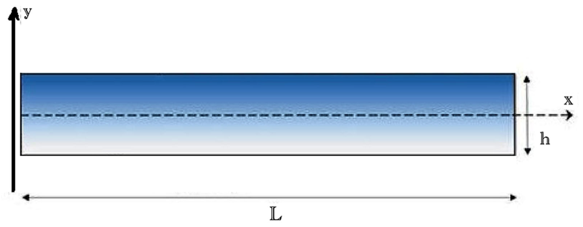
Figure 2.
Boundary-element discretization of the considered structure, showing boundary nodes/elements and internal collocation points.
Figure 2.
Boundary-element discretization of the considered structure, showing boundary nodes/elements and internal collocation points.
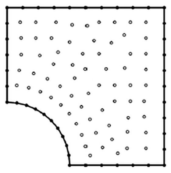
Figure 3.
Effect of the fractional-order parameter on the thermal-stress component versus .
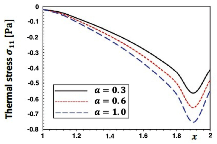
Figure 4.
Effect of the fractional-order parameter on the thermal-stress component versus .
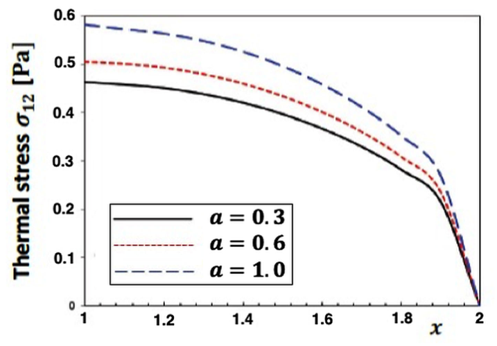
Figure 5.
Effect of the fractional-order parameter on the thermal-stress component versus .
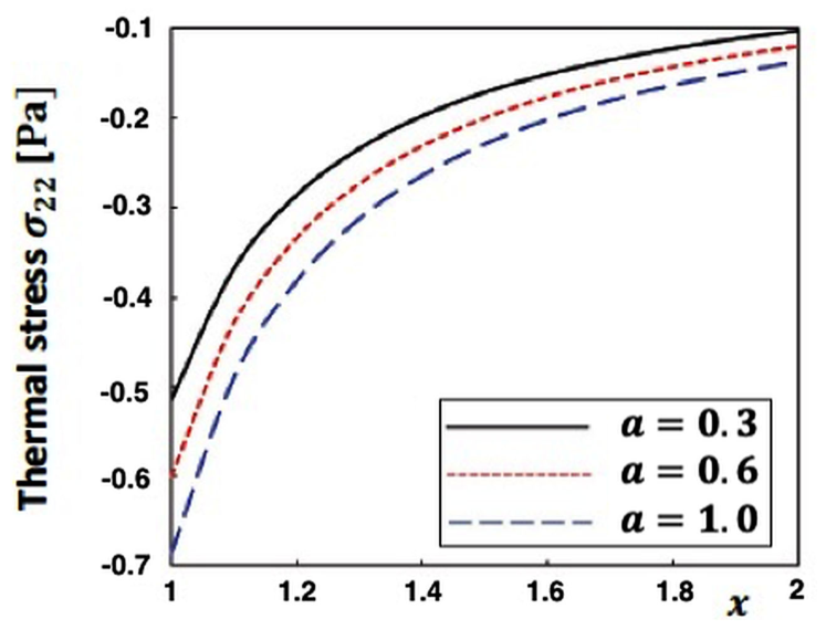
Figure 6.
The influence of the parameter
, related to the functional grading of the material, on the thermal stress component
as a function of
().
Figure 6.
The influence of the parameter
, related to the functional grading of the material, on the thermal stress component
as a function of
().
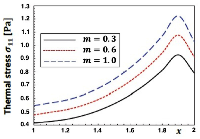
Figure 7.
The influence of the parameter m, related to the functional grading of the material, on the thermal stress component as a function of ().
Figure 7.
The influence of the parameter m, related to the functional grading of the material, on the thermal stress component as a function of ().
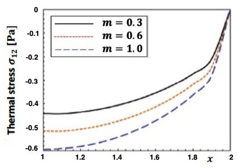
Figure 8.
The influence of the parameter m, related to the functional grading of the material, on the thermal stress component as a function of ().
Figure 8.
The influence of the parameter m, related to the functional grading of the material, on the thermal stress component as a function of ().
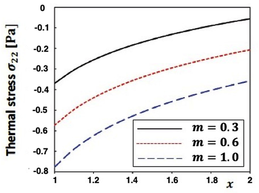
Figure 9.
Special-case comparison of obtained by BEM, GFDM, and FEM–NMM for and (homogeneous case).
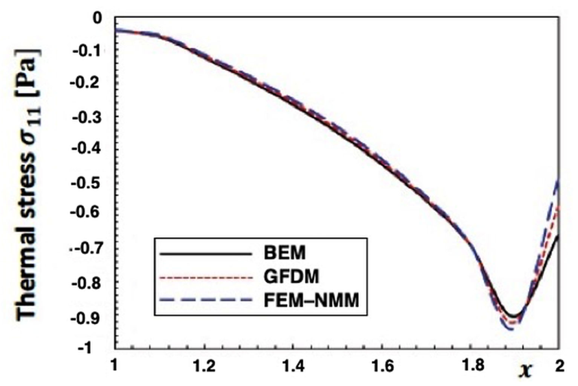
Figure 10.
Special-case comparison of obtained by BEM, GFDM, and FEM–NMM for and (non-homogeneous case).
Figure 10.
Special-case comparison of obtained by BEM, GFDM, and FEM–NMM for and (non-homogeneous case).
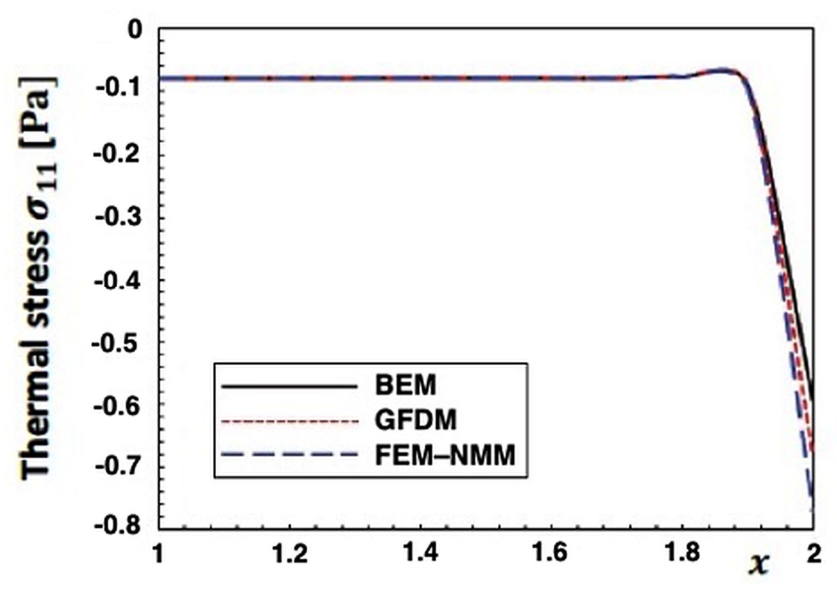

Table 1.
Reported computational-resource and accuracy metrics for the BEM, GFDM, and FEM–NMM implementations.
Table 1.
Reported computational-resource and accuracy metrics for the BEM, GFDM, and FEM–NMM implementations.
| Metric | BEM | GFDM | FEM–NMM |
|---|---|---|---|
| Number of nodes | 68 | 50000 | 48000 |
| Number of elements | 42 | 20000 | 18000 |
| CPU time (reported units) | 2 | 200 | 180 |
| Memory (reported units) | 1 | 180 | 160 |
| Disk space (reported units) | 0 | 240 | 220 |
| Accuracy metric (reported) | 1 | 2.2 | 2.0 |
Disclaimer/Publisher’s Note: The statements, opinions and data contained in all publications are solely those of the individual author(s) and contributor(s) and not of MDPI and/or the editor(s). MDPI and/or the editor(s) disclaim responsibility for any injury to people or property resulting from any ideas, methods, instructions or products referred to in the content. |
© 2026 by the authors. Licensee MDPI, Basel, Switzerland. This article is an open access article distributed under the terms and conditions of the Creative Commons Attribution (CC BY) license (http://creativecommons.org/licenses/by/4.0/).
Copyright: This open access article is published under a Creative Commons CC BY 4.0 license, which permit the free download, distribution, and reuse, provided that the author and preprint are cited in any reuse.