

Submitted:
01 September 2026
Posted:
01 September 2026
You are already at the latest version
Abstract
The added battery mass of electric vehicles intensifies the comfort–road-holding conflict of passive suspensions, while experimentally validated magnetorheological (MR) damper models for production electric vehicles remain scarce. This study characterizes an MR damper designed as a direct replacement for the front strut of a compact electric SUV and validates its quasi-steady simulation model. A single-degree-of-freedom slider–crank test rig was developed in which the piston velocity is reconstructed kinematically from the known crank geometry, thereby avoiding numerical differentiation of a measured displacement signal. A two-stage experimental campaign was conducted: a Taguchi L9 screening identified the control current as the most influential of the three tested factors, and a subsequent 25-point full-factorial matrix spanning peak piston velocities of 0.1–0.3 m/s and coil currents of 0–2.0 A provided the validation data set. A modified Bingham model—with the yield force calibrated by finite-element magnetostatic analysis and the viscous coefficient identified from the 0 A baseline—reproduced the measured force–velocity characteristics with a mean deviation of 10.7% at 0.5 A and 18.6% in deep magnetic saturation; the physical mechanisms responsible for the residual deviation are identified and model refinements are proposed; the validated model is intended as a plant-level foundation for the semi-active and data-driven suspension controllers required by electrified vehicle platforms.
Keywords:
magnetorheological damper
; semi-active suspension
; electric vehicle
; Bingham model
; Taguchi method
; actuator control
1. Introduction
Battery-electric vehicles impose vibration-control requirements that differ substantially from those of conventional vehicles. The traction battery typically increases the kerb mass by 200–400 kg and lowers the ratio of sprung to unsprung mass, while the absence of engine masking noise sharpens occupant sensitivity to road-induced vibration in the 0.5–20 Hz band that governs comfort perception [1]. Passive dampers, whose force–velocity characteristic is fixed at the design stage, cannot simultaneously satisfy the conflicting demands of ride comfort—low damping around the 1–2 Hz body resonance—and road holding, which requires high damping around the 10–15 Hz wheel-hop resonance [1,2].
Semi-active suspensions bridge this gap by modulating the dissipative force in real time without injecting energy into the system [3]. Among the available actuator technologies, magnetorheological (MR) dampers are particularly attractive: the apparent yield stress of the MR fluid responds to the applied magnetic field within milliseconds, the electrical power demand is modest, and the device remains a stable, purely dissipative element in the event of power or control failure, an intrinsic fail-safe property relevant to fault-tolerant actuator design [4]. Since the phenomenological model of Spencer et al. [5] and the material characterization of Jolly et al. [6], a large body of work has addressed MR damper design optimization [7,8], hysteresis modeling [9], semi-active control synthesis [3,10], and, more recently, MR damper configurations dedicated to electrified and low-floor vehicle architectures [2,16].
Nevertheless, three gaps remain. First, most published damper characterizations concern devices designed for generic passenger cars or commercial MR dampers; experimental data for MR dampers designed under the packaging constraints of a specific production battery-electric vehicle are rare. Second, laboratory characterization commonly relies on servo-hydraulic exciters that impose sinusoidal displacement, from which velocity must be reconstructed by numerical differentiation—a procedure that amplifies high-frequency noise and distorts the force–velocity loop near velocity reversal [11]; crank-based rigs that avoid differentiation exist but are less commonly reported in the MR damper literature. Third, for the emerging Vietnamese automotive industry, no experimentally validated MR damper model exists for a domestically produced electric vehicle, which prevents credible simulation-based development of semi-active suspension controllers for these platforms.
The purpose of this study is to close these gaps through the experimental characterization and model validation of an MR damper designed as a direct replacement for the front MacPherson strut damper of the VinFast VF e34, a compact electric SUV produced in Vietnam. The contributions are fourfold: (i) a low-cost single-degree-of-freedom (1-DOF) test rig based on a slider–crank mechanism is designed and commissioned, in which the piston velocity is reconstructed kinematically from the known crank geometry, substantially reducing differentiation-induced noise compared with displacement-sensor-based methods; (ii) a two-stage experimental design—Taguchi L9 screening with analysis of variance (ANOVA) followed by a 25-point full characterization matrix—is executed, with the L9 screening identifying the control current as the most influential of the three tested factors; (iii) a modified Bingham model, with the yield force calibrated from two-dimensional finite-element magnetostatic analysis and the viscous coefficient identified from the 0 A baseline, is validated level by level over the full operating envelope; and (iv) the physical mechanisms responsible for the residual deviation in the saturation regime are identified, and model refinements are proposed.
The remainder of this paper is organized as follows. Section 2 summarizes the damper design and the theoretical model. Section 3 describes the test rig, instrumentation, experimental design, and data processing. Section 4 presents the results and the simulation–experiment comparison. Section 5 concludes the paper.
2. MR Damper Design and Theoretical Model
2.1. Damper Configuration and Design Constraints
The target vehicle employs an independent MacPherson front suspension and a torsion-beam rear axle, with a kerb mass of 1554 kg, a wheelbase of 2611 mm, and an unladen ground clearance of 180 mm. The MR damper was therefore designed as a monotube device dimensionally interchangeable with the original passive strut damper, so that no modification of the body-side or knuckle-side attachments is required. The principal geometric parameters of the designed MR valve and piston assembly are listed in Table 1.
The working fluid is the commercial magnetorheological fluid Bohai A186, selected on the basis of its field-dependent yield stress, its off-state viscosity in the shear-rate range relevant to automotive dampers (γ̇ up to 1000 s−1), and its cost advantage over established alternatives—an important consideration for localization in emerging markets—and its availability as a commercial product of Bohai Advanced Materials Technology Co., Ltd. The magnetic circuit (piston core, flux ring, cylinder) uses AISI 1008 low-carbon steel, selected for its high saturation flux density and low coercivity.
2.2. Quasi-Steady Valve Model and Modified Bingham Formulation
In the annular valve, the pressure drop of the MR fluid modeled as a Bingham plastic comprises a viscous and a field-dependent yield contribution [7,12]:
where η is the plastic viscosity, Q the volumetric flow rate through the gap, b the mean circumference of the annulus, τy(B) the field-dependent yield stress of the fluid, and c ∈ [2, 3] a flow-shape coefficient depending on the ratio of yield to viscous pressure drop. Multiplying by the effective piston area yields the damper force as the sum of a viscous component, proportional to piston velocity, and a controllable component governed by the coil current through τy(B).
For system-level simulation and controller synthesis, the damper force is expressed by a modified Bingham model. The signum discontinuity of the classical Bingham model at zero velocity causes numerical convergence failures in variable-step solvers; it is regularized with a Papanastasiou-type exponential smoothing [13]:
where c0 is the equivalent viscous coefficient, Fy(I) the current-dependent yield force, m the smoothing exponent, and Ff a constant friction offset. The model contains four adjustable quantities: c0 is identified from the slope of the measured force–velocity characteristic at 0 A (passive baseline); Fy(I) is obtained from the finite-element magnetostatic calibration (Section 2.3) without fitting to force data; m controls the sharpness of the velocity-reversal transition and is set to reproduce the near-zero-velocity behavior observed in the rig; and Ff accounts for seal and guide friction. This structure retains the physical separation between the passive (viscous) and controllable (field) force components, keeps the computational cost compatible with real-time semi-active control, and—unlike Bouc–Wen-type hysteresis operators [5,9]—requires no differential-equation states to be integrated online.
2.3. Electromagnetic Calibration of the Yield Force
The mapping from current to flux density, yield stress, and yield force was established by two-dimensional axisymmetric magnetostatic finite-element analysis (Ansys Maxwell 2D) of the valve geometry of Table 1. The B–H characteristic of the low-carbon steel core (AISI 1008) was taken from published material-property databases; because no manufacturer B–H curve is published for the Bohai A186 fluid, a representative curve reported for a comparable iron-particle, hydrocarbon-based commercial MR fluid was adopted as a working assumption for the magnetostatic simulation. A Dirichlet boundary condition (zero vector potential) was applied at the outer boundary of the computational domain. For the nominal 1.0 mm gap, the flux density in the active gap reached 0.735 T at the maximum analyzed excitation, with the flux path confined to the working gap and limited fringing at the pole edges. The predicted damper force increases nearly linearly with flux density up to approximately 0.46 T (force levels of 160–220 N at maximum piston velocity), enters a transition region around 0.60 T (about 300 N), and saturates at approximately 400 N for a flux density of about 0.69 T, where magnetic saturation of the core and rheological saturation of the fluid coincide. This simulated force–current envelope constitutes the model prediction validated experimentally in Section 4.
3. Experimental Method
3.1. Test Rig
Figure 1 shows the 1-DOF damper test rig. A three-phase electric motor drives a 40:1 worm-gear reducer whose output shaft carries a slider–crank mechanism; the connecting rod imposes a reciprocating translation on the damper piston rod. For a crank radius r and connecting-rod length l, the instantaneous piston displacement and velocity are x(θ) = r·cosθ + √(l2 – r2·sin2θ) and v(θ) = –rω·sinθ·[1 + r·cosθ/√(l2 – r2·sin2θ)], respectively, where ω is the constant angular velocity of the crank. The motion is therefore near-sinusoidal, not constant-velocity; each test condition is characterized by the peak piston velocity v_peak = rω (attained near θ = 90°) and the stroke amplitude 2r. The damper is mounted vertically in series with an S-type load cell between the crosshead and the fixed frame. Adjusting the motor speed and the crank radius sets the peak velocity and the stroke amplitude independently. Compared with servo-hydraulic exciters, the rig is at least an order of magnitude less expensive; its main limitation—the inability to impose a truly constant piston velocity—is discussed in Section 4.6.
3.2. Instrumentation and Data Acquisition
The instrumentation chain, whose signal flow is summarized in Figure 2, comprises: (i) an S-type load cell (accuracy ±0.05% full scale) measuring the axial damper force, conditioned by a JY-S60 amplifier; (ii) an incremental encoder (1000 pulses/rev) on the crank shaft, from which the piston position and velocity are reconstructed using the kinematic relations of Section 3.1; (iii) a PeakTech P 1535 programmable DC power supply (0–20 A, 1–32 V) providing the coil current in the range 0–2.0 A; and (iv) a Hantek 1008C eight-channel acquisition unit (2.4 MSa/s) combined with a microcontroller board streaming synchronized data to a computer. Because the crank kinematics are known analytically, the piston velocity is obtained without numerical differentiation of a measured displacement signal, substantially reducing the noise amplification that affects servo-hydraulic test systems [11]. The residual velocity uncertainty is governed by the encoder resolution and the accuracy of the crank-geometry dimensions.
3.3. Experimental Design
The campaign was organized in two stages. In the first stage, a Taguchi L9 orthogonal array (three factors × three levels: stroke amplitude, crank speed, coil current) was executed to screen the relative influence of the operational factors on the damping force. The signal-to-noise ratios and the subsequent ANOVA (Section 4.3) provide an approximate ranking of factor contributions; however, because the L9 array with three three-level factors is saturated and confounds all two-factor interactions with main effects, the resulting variance-contribution percentages should be interpreted as indicative screening estimates rather than exact decompositions.
In the second stage, guided by the screening result, a full-factorial matrix of 25 combinations was executed: five peak piston velocities (0.10, 0.15, 0.20, 0.25, 0.30 m/s) crossed with five current levels (0, 0.5, 1.0, 1.5, 2.0 A). Because the slider–crank mechanism produces a near-sinusoidal velocity profile (Section 3.1), the reported velocities are peak values attained near mid-stroke; the force samples used for averaging are extracted from the portion of each cycle in which the instantaneous velocity lies within ±5% of the peak value. The velocity range covers the dominant operating range of the target front suspension; the current range spans the linear, transition, and saturation regimes identified by the electromagnetic analysis. At each combination, compression and rebound forces were recorded over 5–10 steady cycles.
The test procedure followed a standardized sequence: (1) mounting and alignment of the damper with verification of coaxiality; (2) warm-up cycling at zero current until the fluid temperature stabilized, to standardize viscosity and static-friction conditions; (3) setting of the velocity–current combination; and (4) steady-state data acquisition over multiple cycles. No separate blank-rig runs (damper removed) were performed to isolate the parasitic friction of the crosshead guides; consequently, the measured force includes a small contribution from rig friction, whose effect on the model comparison is discussed in Section 4.5.
3.4. Data Processing
Raw force signals were processed in four steps. First, a scalar Kalman filter suppressed broadband measurement noise, using a random-walk state-transition model appropriate for a directly measured, non-kinematically-predicted force signal (state-transition coefficient A = 1, observation coefficient H = 1, no control input), initialized from a zero force estimate with unit error covariance (x0 = 0, P0 = 1.0); the measurement-noise covariance was set from the load-cell accuracy (R = σv2 ≈ 0.25–1.0) and the process-noise covariance in the range Q ≈ 10−3–10−2, a compromise that smooths local noise spikes without introducing the phase lag typical of low-pass filtering or distorting the force–velocity loop. Second, the static offset of the force channel, identified with the rig at rest, was subtracted. Third, for each test the time intervals in which the instantaneous piston velocity was within ±5% of the target peak value were identified, and the corresponding filtered force samples were extracted. Fourth, the representative compression and rebound forces were computed as arithmetic means over those intervals:
Two performance indices were defined. The first is the energy dissipated per cycle, evaluated numerically as the area of the force–displacement loop; this index is not reported in the present paper because the quasi-sinusoidal velocity profile of the crank rig complicates direct comparison with constant-velocity references, and will be addressed in a future study using full hysteresis-loop measurements. The second is the dynamic range,
which measures the controllability of the damper at a given velocity.
4. Results and Discussion
4.1. Measured Force Characteristics
Table 2 reports the mean compression and rebound forces for all 25 combinations, and Figure 3 plots the corresponding force–velocity characteristics per stroke direction. Three trends are evident. First, at constant current the force increases monotonically with piston velocity, reflecting the viscous term of the Bingham model: at 1.0 A, the compression force rises from 158 N at 0.10 m/s to 340 N at 0.30 m/s. Second, at constant velocity the force increases with current up to 1.0 A; between 1.0 and 2.0 A the compression force stagnates or decreases slightly (e.g., 295 N at 1.0 A versus 270 N at 1.5 A and 280 N at 2.0 A for 0.20 m/s), a signature of combined magnetic–rheological saturation and possible thermal effects that are discussed further in Section 4.5. Third, a systematic compression–rebound asymmetry is observed, with the ratio ranging from approximately 1.0 at 0.30 m/s (where compression and rebound forces nearly converge) to 2.1 at 0.10 m/s, the asymmetry being most pronounced at low velocities. This asymmetry is attributable to the different pressurized volumes and to check-valve-free monotube flow conditions.
The dynamic range computed from Table 2 lies between 1.20 and 1.33 depending on velocity and stroke direction, with the maximum controllable force authority obtained at 1.0 A. While modest compared with laboratory prototypes optimized for force ratio, this range is consistent with the compact valve geometry imposed by the MacPherson packaging constraint and may be sufficient for skyhook-type semi-active control, whose benefit derives primarily from switching between the on- and off-state characteristics around the body resonance [3,10]. Whether the measured dynamic range is adequate for the target vehicle requires verification through closed-loop simulation and road testing.
4.2. Force–Current Relationship and Saturation
The measured force–current characteristic confirms the envelope predicted by the finite-element analysis (Section 2.3): a quasi-linear regime up to approximately 0.5–1.0 A, a transition region with decreasing sensitivity, and a saturation plateau beyond 1.5 A in which additional current produces no useful force increase while adding resistive heating of the coil. From a control-design perspective, this defines the effective operating envelope of the damper: control allocation should be confined below the saturation knee to avoid both wasted energy and potential thermal effects on the MR fluid.
4.3. Factor Ranking by Taguchi–ANOVA
The ANOVA of the first-stage Taguchi L9 array identified the coil current as the most influential of the three tested factors. Because the L9 design with three three-level factors is saturated, all two-factor interactions are confounded with main effects, and the variance-contribution percentages should be regarded as screening estimates rather than exact decompositions. Subject to this caveat, the ANOVA attributes approximately 73% of the observed force variance to the coil current, with stroke amplitude and crank speed together accounting for the remainder. This result carries two practical implications. First, it supports the premise of semi-active MR control by indicating that the field-dependent yield term is the principal force modulation channel within the tested ranges. Second, it is consistent with the structure of the modified Bingham model of Eq. (2), in which the current enters only through the yield force Fy(I) while the viscous coefficient c0 remains constant.
4.4. Simulation–Experiment Comparison
The model of Section 2, with the yield force calibrated from the electromagnetic simulation and the viscous coefficient c0 identified from the 0 A force–velocity slope, was compared with the measured force–velocity characteristics at each non-zero current level. At each current, the comparison was evaluated at the five peak velocities for both compression and rebound strokes, supplemented by two near-reversal points extracted from the continuous force–velocity trace, yielding twelve comparison points per current level. Figure 4 shows the comparison at the four excitation currents, Table 3 summarizes the statistics of the absolute percentage deviation ΔF (%), and Figure 5 visualizes their distribution.
At 0.5 A the model reproduces the measurements with a mean absolute error of 12.5 N (mean percentage deviation 10.7%, median 7.1%), with a single outlier near the velocity-reversal region where static friction and fluid compressibility dominate. The mean absolute error rises to 26.7 N at 1.0 A (15.97% mean deviation), 29.2 N at 1.5 A (18.6% mean deviation), and 26.7 N at 2.0 A (17.6% mean deviation); at every current level the model reproduces the characteristic plateau forces at mid-velocity with deviations below 2%. However, the deviation grows and its dispersion widens as the magnetic circuit enters deep saturation: the standard deviation of ΔF remains near 10.6–11.1% at every current level but rides on a higher mean, so the ±1σ envelope in Figure 5b widens in absolute terms, and at 1.5–2.0 A five of the twelve comparison points per level exceed 20% deviation. The qualitative discrepancy is systematic—the simulated force–velocity plateau is nearly flat, reflecting ideal saturation, whereas the measured plateau is tilted and slightly asymmetric between compression and rebound.
4.5. Error Mechanisms and Model Refinement
Four physical mechanisms, none of which is represented in the quasi-steady Bingham formulation, explain the residual deviation. The first is soft rheological saturation: the yield stress of the fluid does not saturate abruptly, so the measured force–current curve bends gradually, whereas the calibrated yield-force map inherits the sharper saturation of the magnetostatic solution. The second is rig friction: Coulomb friction in the crosshead guides and pin joints adds a velocity-sign-dependent force not present in the model, dominating the relative error at the lowest velocity, where the total force is small; because no blank-rig runs were performed (Section 3.3), this contribution could not be subtracted from the measured data. The third is fluid compressibility and entrained gas: near velocity reversal, compliance of the fluid column softens the force transition, producing the outliers at the extremities of the force–velocity loop. The fourth is a hypothesized thermal effect: sustained cycling at 1.5–2.0 A is expected to heat the coil and the fluid, and the resulting drop in yield stress and viscosity would tilt the measured plateau and reduce the peak force over successive cycles—consistent with the slight force decrease observed between 1.0 A and 1.5–2.0 A in Table 2. However, no direct temperature measurement of the MR fluid was performed in this study, so the thermal-softening hypothesis remains unverified and is proposed as a subject for future investigation.
Accordingly, three refinements are proposed for future work: (i) replacing the yield-force map by a smoothly saturating function of current fitted to the measured knee, e.g., Fy(I) = Fy,∞(1 − e^(−αI)); (ii) augmenting the model with a Coulomb friction term Ff·sgn(v) identified from zero-current blank-rig tests; and (iii) introducing a first-order thermal state coupling coil temperature to a yield-stress reduction factor. Implementation and quantitative assessment of these refinements are left to a follow-up study.
4.6. Comparison with the Literature and Limitations
The validated accuracy (mean deviation 10.7–18.6%, plateau errors below 2%) is comparable to published quasi-steady model validations of automotive MR dampers [7,14,15], while being obtained with a simpler model calibrated without force-data fitting—a potential advantage for design-stage prediction. Limitations of the present study should be noted. (i) The slider–crank mechanism produces a near-sinusoidal velocity profile rather than a truly constant velocity; the reported forces are averaged over the near-peak-velocity portion of each cycle, introducing an averaging effect that a constant-velocity test would avoid. (ii) The model comparison excludes the 0 A condition, so the passive-baseline fit is not independently verified. (iii) No blank-rig tests were conducted; consequently, the crosshead friction force is embedded in the measured damper force. (iv) No repeatability or uncertainty analysis is reported: error bars, confidence intervals, and cycle-to-cycle variability would strengthen the statistical basis of the model validation. (v) The velocity range (up to 0.3 m/s) covers ride but not severe pothole events. (vi) Fluid temperature was not measured, so the thermal-softening hypothesis is unverified. (vii) The characterization is quasi-steady; the millisecond-scale field-response transient was not identified. (viii) Experimental force–displacement and force–velocity hysteresis loops, which would allow direct assessment of energy dissipation and velocity-reversal behavior, are not presented. These aspects, together with on-vehicle road testing per ISO 8608 [17] and comfort evaluation per ISO 2631-1 [18], are the object of ongoing work, together with the synthesis and hardware-in-the-loop validation of semi-active and fault-tolerant suspension controllers built on the model presented here.
5. Conclusions
This study characterized an MR damper designed as a drop-in replacement for the front strut of a production compact electric SUV on a purpose-built 1-DOF slider–crank test rig, and validated the associated finite-element-calibrated modified Bingham model level by level over the operating envelope. The main findings are summarized as follows:
(1) The slider–crank rig reconstructs the piston velocity kinematically, substantially reducing differentiation-induced noise compared with displacement-sensor-based methods. The rig costs a fraction of a servo-hydraulic installation, making systematic MR damper characterization more accessible to laboratories with limited infrastructure. Its main limitation is the near-sinusoidal velocity profile, which prevents truly constant-velocity testing.
(2) The Taguchi L9 screening identified the coil current as the most influential of the three tested factors within the investigated ranges, supporting the premise that the field-dependent yield force is the principal control channel of the device.
(3) The damper delivers compression forces of 123–340 N over 0.10–0.30 m/s and 0–2.0 A, with a dynamic range of 1.20–1.33 and a compression–rebound asymmetry ratio of approximately 1.0–2.1 (most pronounced at low velocity). The saturation knee lies near 1.0–1.5 A; operation beyond the knee wastes energy and may accelerate thermal effects.
(4) The modified Bingham model—with the yield force from finite-element calibration and the viscous coefficient from the 0 A baseline—reproduces the measured characteristics with a mean deviation of 10.7% at 0.5 A and 18.6% in deep saturation, and reproduces plateau forces within 2%. The identified error mechanisms (soft saturation, rig friction, compressibility, hypothesized thermal effects) suggest directions for model refinement.
The validated model provides an adequate plant description for the preliminary synthesis and simulation of semi-active suspension controllers for the target vehicle, subject to the limitations noted above. Because the model is calibrated from physically interpretable, low-cost tests rather than fitted purely to force data, it is also a plausible baseline plant for data-driven or learning-based semi-active control studies, and for evaluating actuator-level strategies to mitigate the additional vibration introduced by electrified powertrain components. The reported data set may support independent benchmarking of MR damper models, provided the caveats regarding rig friction and the absence of repeatability data are taken into account.
Author Contributions
Conceptualization, L.M.; Methodology, L.M. and C.H.P.; Validation, L.M.; Formal analysis, L.M.; Investigation, L.M.; Writing—original draft, L.M.; Writing—review & editing, C.H.P.; Supervision, C.H.P.
Funding
This research received no external funding.
Data Availability Statement
The data presented in this study are available on request from the corresponding author.
Acknowledgments
Not applicable.
Conflicts of Interest
The authors declare no conflicts of interest.
Abbreviations
The following abbreviations are used in this manuscript:
| MR | Magnetorheological |
| ANOVA | Analysis of Variance |
| FEM | Finite-Element Method |
| DOF | Degree of Freedom |
| SUV | Sport Utility Vehicle |
References
- Savaresi SM, Poussot-Vassal C, Spelta C, et al. Semi-Active Suspension Control Design for Vehicles. Oxford: Butterworth-Heinemann; 2010.
- Wang Z, Liu C, et al. Advancements in Semi-Active Automotive Suspension Systems with Magnetorheological Dampers: A Review. Applied Sciences. 2024; 14(17): article no. 7866. [CrossRef]
- Ahmadian M, Song X, Southward SC. No-Jerk Skyhook Control Methods for Semiactive Suspensions. Journal of Vibration and Acoustics. 2004; 126(4): 580–584. [CrossRef]
- Carlson JD, Jolly MR. MR Fluid, Foam and Elastomer Devices. Mechatronics. 2000; 10(4–5): 555–569. [CrossRef]
- Spencer BF, Dyke SJ, Sain MK, et al. Phenomenological Model for Magnetorheological Dampers. Journal of Engineering Mechanics. 1997; 123(3): 230–238. [CrossRef]
- Jolly MR, Carlson JD, Muñoz BC. A Model of the Behaviour of Magnetorheological Materials. Smart Materials and Structures. 1996; 5(5): 607–614. [CrossRef]
- Hu G, Qi H, Chen M, et al. Optimal Design of Magnetorheological Damper with Multiple Axial Fluid Flow Channels Using BP Neural Network and Particle Swarm Optimization Methodologies. International Journal of Applied Electromagnetics and Mechanics. 2021; 67(3): 339–360. [CrossRef]
- Nguyen QH, Choi SB. Optimal Design of MR Shock Absorber and Application to Vehicle Suspension. Smart Materials and Structures. 2009; 18(3): article no. 035012. [CrossRef]
- Kwok NM, Ha QP, Nguyen TH, et al. A Novel Hysteretic Model for Magnetorheological Fluid Dampers and Parameter Identification Using Particle Swarm Optimization. Sensors and Actuators A: Physical. 2006; 132(2): 441–451. [CrossRef]
- Kim J, Lee T, Kim CJ, et al. Model Predictive Control of a Semi-Active Suspension with a Shift Delay Compensation Using Preview Road Information. Control Engineering Practice. 2023; 137: article no. 105584. [CrossRef]
- Goncalves FD, Ahmadian M, Carlson JD. A Review of the State of the Art in Magnetorheological Fluid Technologies — Part I: MR Fluid and MR Fluid Models. The Shock and Vibration Digest. 2006; 38(3): 203–219.
- Yang G, Spencer BF, Carlson JD, et al. Large-Scale MR Fluid Dampers: Modeling and Dynamic Performance Considerations. Engineering Structures. 2002; 24(3): 309–323. [CrossRef]
- Papanastasiou TC. Flows of Materials with Yield. Journal of Rheology. 1987; 31(5): 385–404. [CrossRef]
- Shiao Y, Jow M, Kuo W, et al. Design and Experiment of the Magnetorheological Damper with Multiple Poles. Applied Mechanics and Materials. 2015; 764–765: 223–227. [CrossRef]
- Ahammed R, Hasan MZ. An FEA and CFD Coupled Numerical Analysis Approach for Characterizing Magneto-Rheological (MR) Grease Damper. Sādhanā. 2023; 48(3): article no. 164.
- Park YJ, Choi SB. A New Rotary Magnetorheological Damper for a Semi-Active Suspension System of Low-Floor Vehicles. Actuators. 2024; 13(4): article no. 155. [CrossRef]
- Mechanical Vibration — Road Surface Profiles — Reporting of Measured Data, ISO 8608:2016, 2016.
- Mechanical Vibration and Shock — Evaluation of Human Exposure to Whole-Body Vibration — Part 1: General Requirements, ISO 2631-1:1997, 1997.
Figure 1.
Single-DOF damper test rig: 1 – load cell; 2 – MR damper; 3 – signal-conditioning unit; 4 – slider–crank mechanism; 5 – electric motor; 6 – gear reducer; 7 – incremental encoder.
Figure 1.
Single-DOF damper test rig: 1 – load cell; 2 – MR damper; 3 – signal-conditioning unit; 4 – slider–crank mechanism; 5 – electric motor; 6 – gear reducer; 7 – incremental encoder.
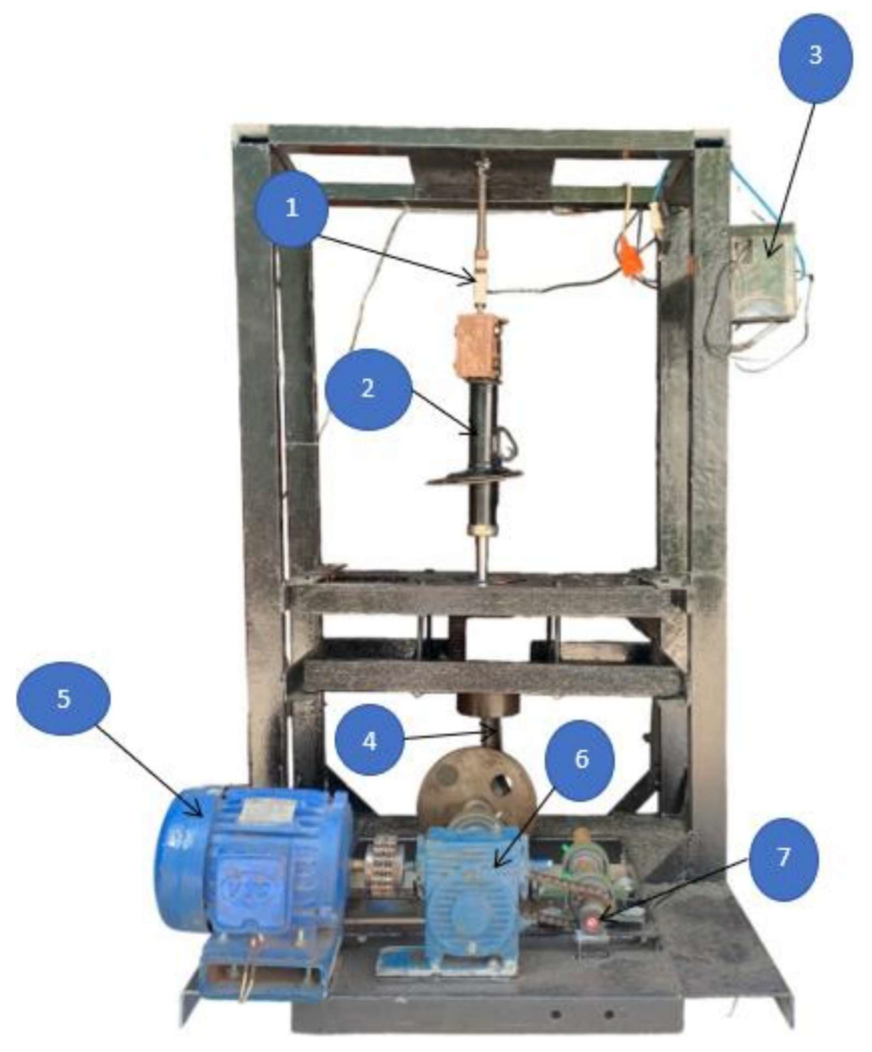
Figure 2.
Signal-flow diagram of the experimental system.
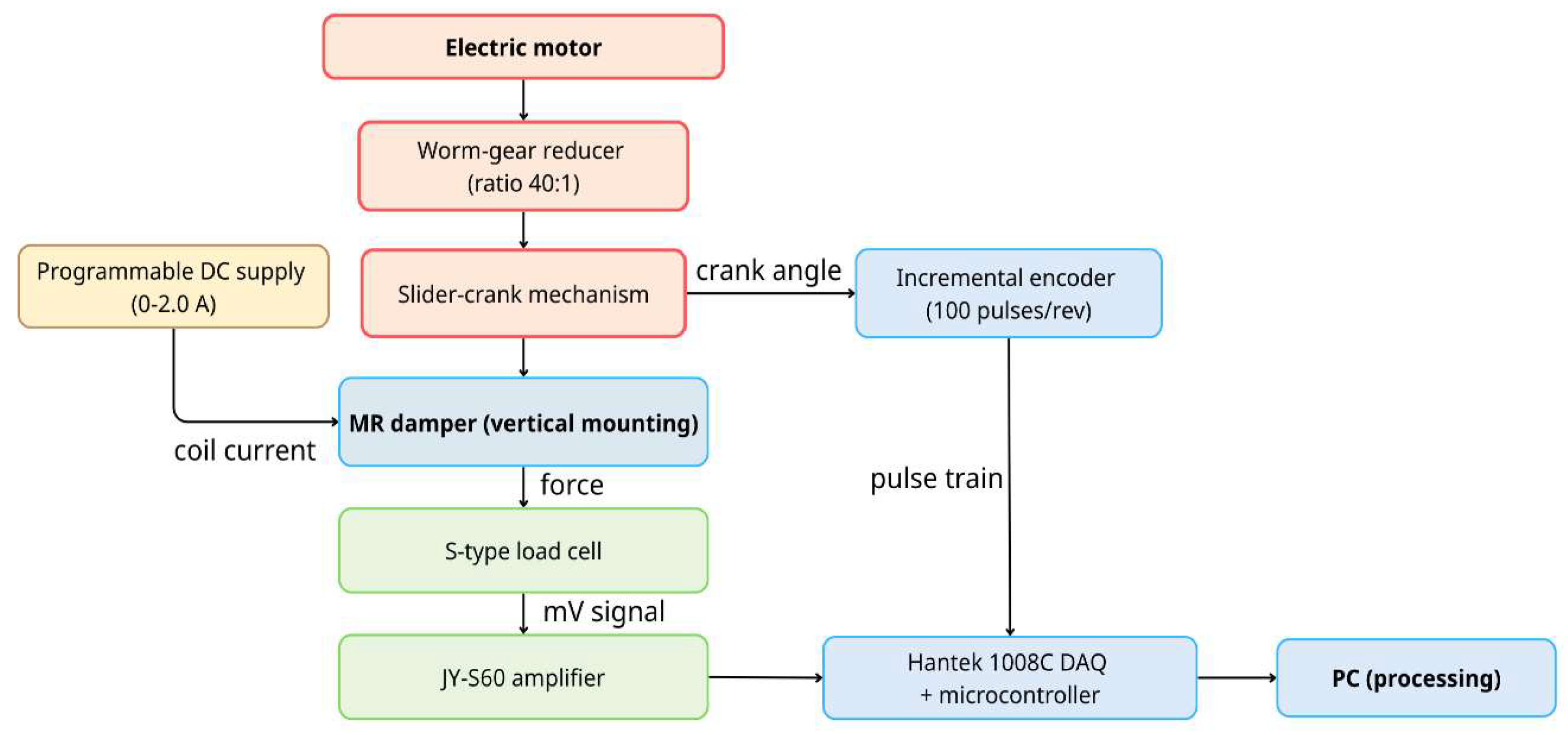
Figure 3.
Measured mean damping force versus piston velocity at coil currents of 0–2.0 A: (a) compression stroke; (b) rebound stroke.
Figure 3.
Measured mean damping force versus piston velocity at coil currents of 0–2.0 A: (a) compression stroke; (b) rebound stroke.
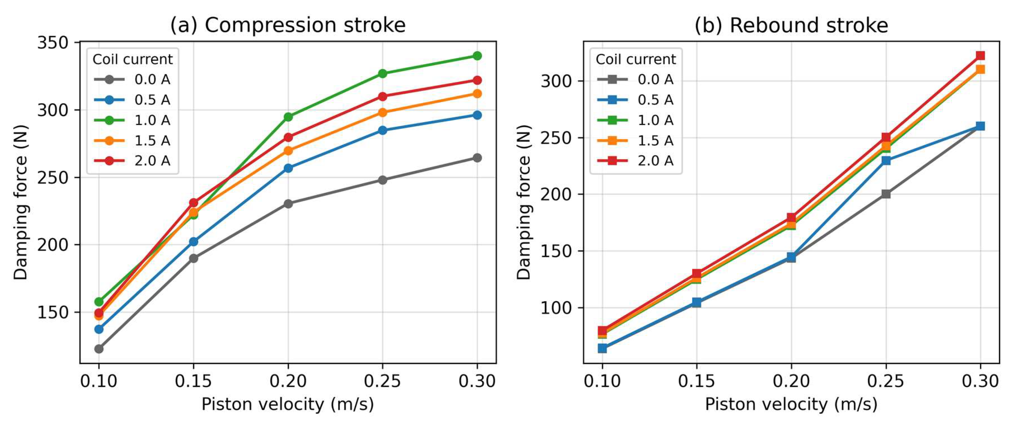
Figure 4.
Model–experiment comparison of the force–velocity characteristics: (a) I = 0.5 A; (b) I = 1.0 A; (c) I = 1.5 A; (d) I = 2.0 A.
Figure 4.
Model–experiment comparison of the force–velocity characteristics: (a) I = 0.5 A; (b) I = 1.0 A; (c) I = 1.5 A; (d) I = 2.0 A.
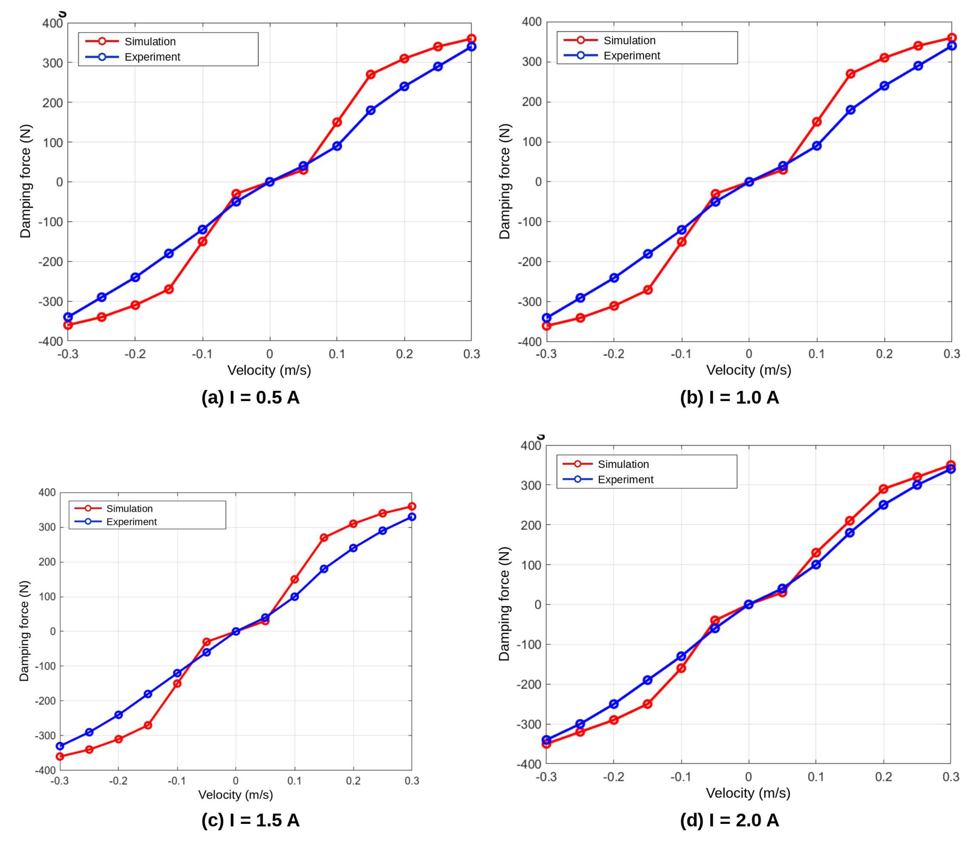
Figure 5.
Statistics of the force deviation ΔF between model and experiment: (a) five-number summary per current level; (b) mean deviation with ±1σ dispersion.
Figure 5.
Statistics of the force deviation ΔF between model and experiment: (a) five-number summary per current level; (b) mean deviation with ±1σ dispersion.
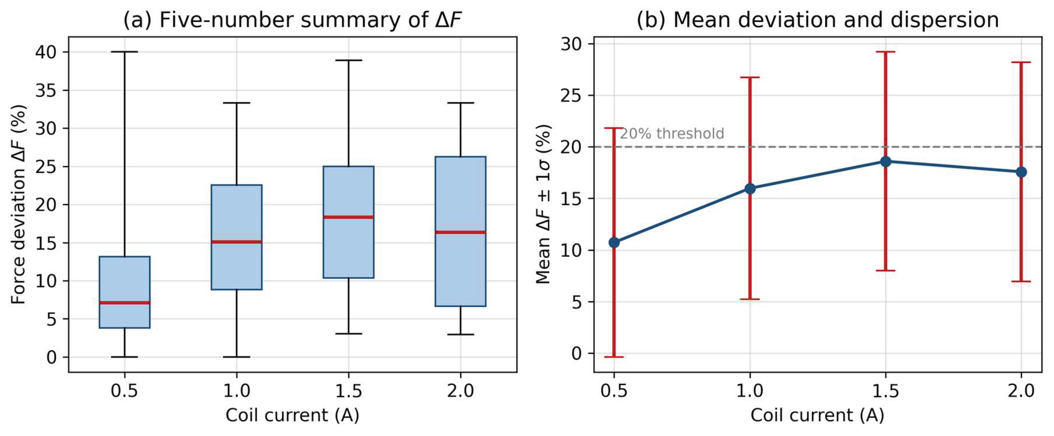

Table 1.
Principal design parameters of the MR damper valve.
| Symbol | Description | Value |
|---|---|---|
| L | Active pole length | 45 mm |
| Ld | Working length of damper | 140 mm |
| W | Coil window width | 33 mm |
| h | Annular working gap | 0.9 / 1.0 / 1.1 mm |
| hd | Pole depth | 6 mm |
| t | Flange thickness | 7.5 mm |
| r1…r4 | Characteristic radii | 5 / 8 / 20.5 / 27.5 mm |
Table 2.
Measured mean damping force (N)—compression/rebound.
| v (m/s) | 0 A | 0.5 A | 1.0 A | 1.5 A | 2.0 A |
|---|---|---|---|---|---|
| 0.10 | 122.9 / 63.8 | 137.4 / 64.3 | 157.7 / 76.6 | 147.4 / 77.3 | 149.6 / 79.8 |
| 0.15 | 189.9 / 104.1 | 202.2 / 104.8 | 222.1 / 125.0 | 224.1 / 126.2 | 231.1 / 130.1 |
| 0.20 | 230.5 / 143.6 | 256.8 / 144.7 | 294.8 / 172.4 | 269.7 / 174.1 | 279.7 / 179.5 |
| 0.25 | 248.0 / 200.1 | 284.7 / 229.7 | 326.8 / 240.3 | 298.0 / 242.6 | 310.0 / 250.2 |
| 0.30 | 264.4 / 260.0 | 296.2 / 260.0 | 340.0 / 309.9 | 312.0 / 310.0 | 322.0 / 322.0 |
Table 3.
Statistics of the force deviation ΔF (%) between model and experiment.
| I (A) | Mean | Std | Min | Q1 | Median | Q3 | Max | Points > 20% |
|---|---|---|---|---|---|---|---|---|
| 0.5 | 10.73 | 11.09 | 0.00 | 3.78 | 7.13 | 13.13 | 40.00 | 2/12 |
| 1.0 | 15.97 | 10.74 | 0.00 | 8.81 | 15.08 | 22.56 | 33.33 | 4/12 |
| 1.5 | 18.59 | 10.59 | 3.03 | 10.34 | 18.34 | 25.00 | 38.89 | 5/12 |
| 2.0 | 17.57 | 10.63 | 2.94 | 6.67 | 16.34 | 26.25 | 33.33 | 5/12 |
Disclaimer/Publisher’s Note: The statements, opinions and data contained in all publications are solely those of the individual author(s) and contributor(s) and not of MDPI and/or the editor(s). MDPI and/or the editor(s) disclaim responsibility for any injury to people or property resulting from any ideas, methods, instructions or products referred to in the content. |
© 2026 by the authors. Licensee MDPI, Basel, Switzerland. This article is an open access article distributed under the terms and conditions of the Creative Commons Attribution (CC BY) license.
Copyright: This open access article is published under a Creative Commons CC BY 4.0 license, which permit the free download, distribution, and reuse, provided that the author and preprint are cited in any reuse.