

Submitted:
06 October 2026
Posted:
09 October 2026
You are already at the latest version
Abstract
We explore the hypothesis that the observed FLRW cosmology admits a finite global completion and ask how this changes the prospects for testing quantum gravity. A finite overdense region embedded in a larger background can undergo gravitational collapse, providing a possible prehistory for the observed expansion. If the collapse approaches a finite quantum-supported density \( \rho_G \), positive spatial curvature permits a nonsingular bounce connecting contraction to expansion. In one realization, the late-time de Sitter horizon of the FLRW interior is identified with the Schwarzschild horizon of the exterior, providing a finite global completion without modifying the local FLRW dynamics. The central proposal of this review is that such a finite bouncing cosmology can act as a laboratory for quantum gravity. We use quadratic gravity and PT-symmetric quantum theory as concrete realizations while emphasizing that the observational strategy is more general. Within scalaron inflation, the measured CMB amplitude constrains the \( R^2 \) coupling \( \alpha \) once the primordial state, reheating history and pivot-scale mapping are specified. Large-angle CMB parity statistics can similarly be related, within a specified primordial-state model, to an effective PT-breaking amplitude \( A_{\rm PT} \). PT completion also suggests a possible connection between the arrow of time and quantum information: information inaccessible within one semiclassical branch may remain encoded in a unitary PT-complete quantum state, potentially reformulating aspects of both the Past Hypothesis and apparent information loss. The contracting phase provides a possible second source of structure, distinct from inflationary quantum fluctuations. Nonlinear structures may form before the bounce. If such relics survive, their evolved abundance and mass function could be constrained by dark matter, early supermassive black holes, lensing and gravitational-wave observations. Strong-gravity measurements provide complementary tests of candidate microscopic completions through black-hole perturbations, horizon absorption and extreme-mass-ratio inspirals whenever the relevant additional degrees of freedom lie in an observationally accessible regime. The resulting framework is therefore best regarded as a network of cross-consistency and falsification tests. Relations among \( A_s \), \( \alpha \), \( A_{\rm PT} \), \( Y_B \), \( \rho_G \), spatial curvature, relic populations and strong-gravity observables range from established model-specific results to phenomenological hypotheses that still require microscopic derivation. If these relations can be sufficiently specified, otherwise unrelated observations could over-constrain a common quantum-gravitational history. Cosmological maps, black holes and gravitational waves can be regarded as experiments performed by Nature in regimes inaccessible to terrestrial laboratories, providing an observational approach to quantum gravity complementary to microscopic theory building. A finite Universe may preserve measurable information about both its pre-Big-Bang evolution and its high-density quantum state, turning otherwise inaccessible quantum-gravitational dynamics into a potentially falsifiable observational programme.
Keywords:
quantum cosmology
; black holes
; quantum field theory in curved spacetime
; gravitational waves
; quasi-normal modes
; isospectrality
; information paradox
; bouncing cosmology
; finite universe
1. Introduction
Understanding how quantum theory and gravity combine to describe the Universe remains one of the central challenges of modern physics. General Relativity is expected to provide the low-energy classical description of gravity, with quantum corrections becoming important at sufficiently high curvature or short distances. Yet the regimes in which such effects become significant are usually assumed to lie far beyond direct experimental reach. This raises a fundamental question: can the Universe itself provide an arena in which quantum-gravitational physics becomes observable?
Many approaches to quantum gravity begin from the microscopic theory and ask how its consequences might eventually become observable. String theory, loop quantum gravity, higher-curvature gravity, non-local theories and other modified descriptions of gravity follow this logic in different ways. The difficulty is that the characteristic energies, curvatures and timescales involved are generally far beyond what can be reproduced in terrestrial experiments.
Cosmology offers a complementary strategy. The Universe has already explored physical regimes that no laboratory on Earth can create: primordial densities and curvatures, horizons extending over cosmological distances, black holes and gravitational fields strong enough to generate observable gravitational waves. Maps of the cosmic microwave background and the large-scale distribution of galaxies, together with observations of black holes and gravitational waves, can therefore be viewed not merely as astronomical data but as experiments performed by Nature. The question is whether these different experiments preserve correlated information about the same underlying quantum-gravitational physics.
The individual ingredients involved in this question have substantial literatures of their own. Bouncing cosmologies have been extensively reviewed [1,2], as have quadratic gravity [3], primordial black holes as dark-matter candidates [4] and strong-gravity tests of compact objects [5]. The purpose of the present review is not to claim originality for these subjects individually. To our knowledge, however, they have not previously been organized within the specific framework developed here: a finite bouncing cosmology in which the high-density quantum state, primordial perturbations, matter–antimatter asymmetry, compact relics, dark matter and strong-gravity observables are treated as potentially related consequences of the same underlying gravitational history. The novelty of the review is therefore primarily synthetic and observational: to ask which of these connections are already calculable, which remain phenomenological and whether sufficiently specified realizations can ultimately be falsified through cross-consistency tests.
The starting point is a global hypothesis: the FLRW cosmology we observe may admit a finite global completion. Present observations do not establish that the Universe is globally finite. They do, however, imply within the standard CDM interpretation a positive cosmological constant and hence a finite asymptotic causal horizon,
The conventional construction continues the same homogeneous FLRW solution indefinitely beyond this horizon. Such a continuation is mathematically consistent, but it represents a choice of global completion rather than an observationally accessible part of the cosmology. An alternative is that the locally observed FLRW region belongs to a finite gravitating spacetime whose exterior completion is different. In the Schwarzschild realization considered here, the asymptotic de Sitter horizon of the interior is identified with the gravitational horizon of the exterior,
The local FLRW dynamics need not change; what changes is the global spacetime to which that cosmology belongs.
The two possibilities are not physically identical. An indefinitely extended FLRW completion extrapolates the same homogeneous state beyond every observer’s causal horizon. A finite completion opens the possibility of a causal formation history. The cosmological region may originate as an overdensity within a larger background, become gravitationally bound and undergo collapse. The observed expanding Universe can then be interpreted not as an isolated initial condition but as the outcome of gravitational evolution.
It is important, however, to separate finiteness from the additional ingredients of this particular construction. Global finiteness alone does not imply positive spatial curvature, gravitational collapse, a bounce or a black-hole horizon. Here we consider the more specific case of a finite, gravitationally bound overdensity. Within this class of models, positive curvature arises naturally from the bound dynamics, while a sufficiently massive and compact region can lie within its own gravitational radius,
Because the mean density required for an object of radius R to satisfy scales as , a cosmological region can lie within its gravitational radius while having a very low mean density. The black-hole character of the Black Hole Universe (BHU) is therefore not a consequence of finiteness alone, but of finite total mass together with the global gravitational configuration.
From this perspective, cosmic expansion need not mark the absolute beginning of the system. During an earlier contracting phase, density and curvature can increase until the classical description ceases to be adequate. If the collapse approaches a finite quantum-supported density , positive spatial curvature can provide a turning point at non-zero scale factor. The Big Bang is then replaced by a transition between a contracting classical phase, a high-density quantum regime and the expanding Universe we observe.
The existence of such a regular homogeneous solution is only the beginning of the problem. It does not establish that the bounce is stable. Shear and other perturbations can grow during contraction, and a viable microscopic completion must demonstrate either that they remain perturbative throughout the finite collapse or that high-density physics modifies their evolution before they backreact strongly on the background. Stability therefore becomes part of the observational and theoretical test of the framework rather than an assumption hidden in the background solution.
The central theme of this review is that the high-density endpoint of a finite gravitational collapse can turn otherwise inaccessible quantum-gravity physics into an observational problem. We do not assume that one particular microscopic theory must provide the correct description. Instead, candidate theories are asked to determine properties of the high-density state—its characteristic scale, stability, perturbation spectrum, symmetry structure and transition to ordinary matter—which can then be confronted with observations at much later times.
Quadratic gravity provides one concrete example. Its sector generates the scalaron dynamics underlying Starobinsky inflation. Within a specified inflationary state and reheating history, the measured scalar amplitude constrains the quadratic coupling and hence a characteristic high-curvature scale. This raises the possibility that the effective bounce density may be related to a coupling already constrained by the CMB. Such an identification is not assumed here: deriving a relation between the scalaron scale and the quantum-supported density remains a microscopic problem and therefore a potential consistency or falsification test.
A second example concerns the quantum state itself. We consider PT symmetry as a possible organizing principle and direct-sum quantization as one explicit realization. In such a description, contracting and expanding semiclassical sectors can belong to a single PT-complete quantum state while carrying opposite time orientations. This possibility opens a connection to two deeper questions. Information carried by the contracting branch need not be destroyed merely because it is inaccessible to an observer in the expanding branch, and the low gravitational entropy conventionally encoded in the Past Hypothesis need not necessarily be imposed as an absolute initial condition. These ideas do not yet provide a microscopic solution to either problem, but they suggest that apparent information loss and the thermodynamic arrow of time may both be properties of the quantum-to-classical transition.
The same transition may leave observable symmetry information. Large-angle CMB temperature fluctuations exhibit an intriguing preference for odd over even multipoles. An even–odd imbalance does not by itself establish statistical parity or PT violation, but within a specified primordial-state model the observed statistics can be compared with predictions of PT-related constructions and represented by an effective symmetry-breaking amplitude . Polarization and tensor observables then provide independent ways of testing that interpretation. If a primordial symmetry bias is transferred to matter during reheating, it may also participate in baryogenesis or leptogenesis, although an actual matter asymmetry still requires charge-sensitive dynamics and baryon- or lepton-number violation.
The contracting phase provides another possible observational record. Gravitational instability can generate nonlinear structures before the high-density transition, distinct from the nearly Gaussian perturbations produced during inflation. Whether such structures survive the bounce is not established by crossing the FLRW apparent horizon: their evolution requires a dynamical transfer prescription through the high-density phase. If a relic population survives, however, its evolved mass function can be confronted with dark-matter constraints, high-redshift massive black holes, lensing and gravitational-wave observations. The relic hypothesis therefore provides another route by which the microscopic bounce can become testable.
Strong-gravity observations offer a complementary probe. Black-hole ringdown, horizon absorption, extreme-mass-ratio inspirals and gravitational waves can test additional gravitational degrees of freedom or modified near-horizon response when the corresponding scales and couplings are observationally accessible. Strong fields alone do not guarantee sensitivity to ultraviolet physics: the response must be calculated within the specific completion. These channels are therefore treated here as research directions and potential consistency tests rather than generic predictions of a finite Universe.
The central strength of the programme is consequently not any single anomaly or proposed signature. It is the possibility that quantities inferred from very different observations—the scalar amplitude , the quadratic coupling , a model-defined , the baryon abundance , the bounce density , spatial curvature, relic populations and strong-gravity observables—may eventually be connected by a smaller set of microscopic parameters. At present these relations have different theoretical status. Some are established within specified models, some are model-dependent calculations and others remain phenomenological hypotheses requiring further dynamics. We make these distinctions explicit and ask what would have to be derived before the framework becomes genuinely over-constrained.
This review develops that programme. We first examine the global gravitational implications of a finite completion and the possibility that the observed expansion follows an earlier phase of collapse. We then discuss the finite-density bounce and its stability requirements. Quadratic gravity is used as a worked example of high-curvature dynamics, followed by PT completion and its possible implications for primordial symmetry, quantum information and the arrow of time. We subsequently consider inflation, reheating, baryogenesis and leptogenesis, the formation and possible survival of pre-bounce relics and strong-gravity and gravitational-wave tests. Finally, we organize these channels into a network of cross-consistency and falsification tests. The aim is not to advocate one unique microscopic theory, but to explore how observations of the Universe can turn quantum gravity from a purely theoretical problem into an empirical programme.
2. A Finite Gravitating Universe
The starting point of the Black Hole Universe (BHU) picture is not the existence of a black hole, but the assumption that the cosmological region we observe is finite. A finite gravitating system differs qualitatively from an idealized infinite FLRW Universe because it possesses a total mass, a characteristic size and a global completion. These properties allow its evolution to be discussed not only locally, through the Friedmann equations, but also globally, as the dynamics of a self-gravitating region embedded in a larger spacetime.
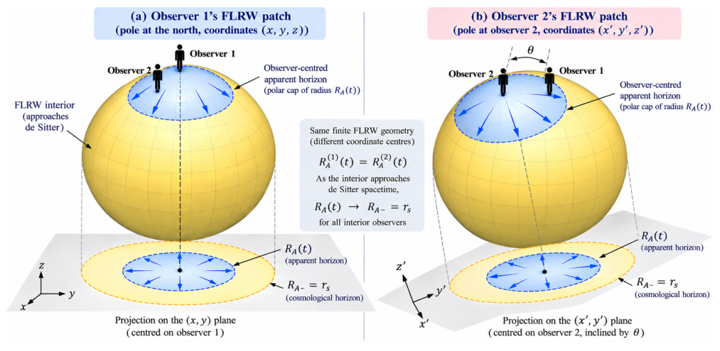
The local cosmological geometry can remain the standard FLRW solution throughout the interior; what changes is its global completion. In a CDM cosmology with the observed positive cosmological constant, the late-time FLRW geometry approaches de Sitter spacetime and each observer is associated with a finite asymptotic causal horizon of radius . The standard construction extends the same homogeneous FLRW solution indefinitely beyond this horizon. An alternative is to complete the finite cosmological region by a Schwarzschild exterior across a common null horizon, . The resulting spacetime has an FLRW cosmological interior and a Schwarzschild black-hole exterior, while preserving the same local FLRW dynamics accessible to interior observers. This finite global completion is illustrated in Figure 1. An explicit construction realising the corresponding null matching is presented in [6]; the details of that construction are not essential for the present review. The relevant point here is simply that the observed CDM FLRW geometry admits such a finite global completion. A natural formation mechanism is then provided by gravitational instability: an initially bounded overdensity within a larger background can collapse within its own gravitational radius and generate the finite cosmological region.
Gravity is attractive, so sufficiently overdense regions tend to decouple from the surrounding expansion and collapse [7,8]. The same mechanism operates on familiar scales in the formation of bound structures such as stars and halos (see later §8.1 and Figure 7). The BHU proposal extends this logic to the largest possible scale: the cosmological region that later becomes our observable Universe may itself originate from the gravitational collapse of a finite perturbation in a parent background.
This does not require the parent spacetime to play an observational role in the subsequent evolution. Once the overdense region becomes causally isolated, its internal dynamics can be described independently. The essential point is that the observed expanding phase need not represent the absolute beginning of the system. It may instead correspond to the post-bounce evolution of a finite region that previously contracted.
Figure 1.
Observer-centred causal patches in a finite FLRW geometry. (a) A lower-dimensional embedding representation centred on Observer 1. The yellow spherical surface represents the finite FLRW interior, while the blue polar cap denotes the region inside that observer’s instantaneous apparent horizon. The projection onto the auxiliary plane shows the corresponding areal radii explicitly: the blue circle has radius , while the outer yellow circle represents the asymptotic de Sitter scale . As the interior approaches de Sitter spacetime, . (b) Different observers define different, generally overlapping apparent-horizon patches of the same homogeneous geometry. Observers 1 and 2 therefore need not see precisely the same events, but homogeneity guarantees that at the same cosmic time they obtain the same horizon radius, . Neither observer defines a preferred centre and neither apparent horizon is a material edge of space. In the asymptotic limit all observer-centred horizon scales approach the same invariant value , selected by the global Schwarzschild completion. The embedding and projection coordinates are auxiliary visualisation devices and do not represent additional physical dimensions.
Figure 1.
Observer-centred causal patches in a finite FLRW geometry. (a) A lower-dimensional embedding representation centred on Observer 1. The yellow spherical surface represents the finite FLRW interior, while the blue polar cap denotes the region inside that observer’s instantaneous apparent horizon. The projection onto the auxiliary plane shows the corresponding areal radii explicitly: the blue circle has radius , while the outer yellow circle represents the asymptotic de Sitter scale . As the interior approaches de Sitter spacetime, . (b) Different observers define different, generally overlapping apparent-horizon patches of the same homogeneous geometry. Observers 1 and 2 therefore need not see precisely the same events, but homogeneity guarantees that at the same cosmic time they obtain the same horizon radius, . Neither observer defines a preferred centre and neither apparent horizon is a material edge of space. In the asymptotic limit all observer-centred horizon scales approach the same invariant value , selected by the global Schwarzschild completion. The embedding and projection coordinates are auxiliary visualisation devices and do not represent additional physical dimensions.
2.1. Closed Geometry and Global Collapse
The local interior can remain the ordinary FLRW spacetime throughout its evolution. What changes is its global completion. In the conventional interpretation the homogeneous FLRW solution is continued beyond each observer’s cosmological horizon. In the construction considered here, the late-time FLRW interior instead approaches a de Sitter geometry whose event horizon is identified with the Schwarzschild event horizon of the exterior,
There is consequently no intermediate empty shell inside the cosmological region and no material edge that an interior observer could encounter.
This distinction can be understood geometrically. A closed FLRW spatial section expands or contracts intrinsically, in the same way that the surface of a sphere changes size without leaving an empty annulus behind it. The finite completion is therefore not a Newtonian ball of matter moving through a pre-existing empty space. The FLRW geometry itself is the interior spacetime, while the Schwarzschild vacuum provides its global exterior completion across the asymptotic null horizon.
The closed geometry is important because it provides the global contribution required for a turning point. The Friedmann equation may be written as
where the positive spatial curvature term enters with the opposite sign to the matter density. During contraction the density generally increases, but if the high-density state approaches a finite value, the curvature term can balance the energy density at a non-zero scale factor and permit
This is the basic geometrical condition required for a bounce.
The role of positive curvature should not be confused with finiteness itself. A compact space can in principle have zero or negative curvature. The physical statement relevant here is narrower: a finite overdense region produced by gravitational collapse naturally behaves as a closed system with positive curvature. In the Newtonian description of a spherical perturbation, this corresponds to a gravitationally bound system with negative total energy. Within this class of models, the curvature term provides the global contribution that allows contraction to reverse into expansion.
2.2. Why a Cosmological-Scale Region Can Become a Black Hole
The term “Black Hole Universe” can initially sound much more exotic than the underlying geometry actually requires. For a spherical region of radius R and mean density , the enclosed Misner-Sharp mass M is [8]:
The condition that the region lies within its own gravitational radius, , gives
The important feature is the scaling
The larger the system, the smaller the mean density required for its gravitational radius to exceed its physical size. Stellar black holes are extremely dense because their radii are small. A cosmological black hole can instead have an enormous radius and a correspondingly low mean density.
The black-hole character of the BHU is therefore not introduced as an additional assumption. It follows from the combination of finite total mass and sufficiently large size. In this sense, the central hypothesis is finiteness; the existence of a gravitational horizon is a consequence of the global mass distribution.
This interpretation is especially natural in a system that evolves from collapse to expansion. During the contracting phase the density increases but the completion remains the same. After the bounce, as the density decreases, but the same boundary continues to constrain the global completion. At late times the interior can approach a quasi-de Sitter state set by the gravitational radius of the whole system. The early high-density phase and the late accelerated phase are then not unrelated additions to the cosmological model but different regimes of the same finite gravitational configuration.
The possibility that the observed value of the cosmological constant may encode quantum-gravitational information has a long history [10,11]. Early approaches based on Euclidean quantum gravity attempted to derive a probability distribution for . In particular, Elizalde and Gaztañaga showed that higher-order corrections to the effective action can qualitatively alter the strong preference for obtained in Coleman’s original proposal, producing instead a smooth distribution around zero [12]. The present construction is physically different: is associated with the global boundary of a finite gravitating region rather than selected from a probability distribution. Nevertheless, both approaches illustrate how the observed cosmological constant may be sensitive to physics beyond the classical Einstein action.
2.3. Finiteness as the Organizing Principle
The role of finiteness can now be summarized more precisely. Finiteness by itself does not imply gravitational collapse, positive spatial curvature, a bounce or a black-hole horizon. Rather, it changes the global problem by allowing the cosmological region to possess a finite total mass, a characteristic size and a non-trivial global completion. If that finite region originates as a gravitationally bound overdensity, the sequence considered here can be represented schematically as
These ingredients then open possibilities that are absent, or less directly motivated, in an indefinitely extended homogeneous cosmology. Positive curvature can provide the geometrical contribution required for a turning point if the collapsing density approaches a finite value. A sufficiently compact finite mass can possess a gravitational horizon, while the late-time FLRW interior can admit a global completion different from an indefinite continuation of the homogeneous solution. Pre-bounce structures may also leave observable relics if their evolution through the high-density phase allows them to survive.
The distinction is important. None of these consequences follows from finiteness alone, and none should be regarded as universally required by a finite Universe. They arise within the particular class of finite, gravitationally bound cosmologies considered here. Finiteness is therefore best understood as the organizing principle that makes a global gravitational history possible, while collapse, positive curvature, the horizon structure and the bounce are additional dynamical or geometrical ingredients of the specific realization.
The role of quantum gravity enters at the next step. Classical collapse drives the density and curvature toward a regime in which General Relativity can no longer be assumed to provide a complete description. The fate of the system then depends on the microscopic physics of the high-density state: whether the singularity is avoided, what fixes the limiting density , whether anisotropies and perturbations remain under control, how contraction is connected to expansion and which structures, if any, survive the transition.
It is precisely this separation between global gravitational evolution and microscopic high-density physics that makes a finite gravitating Universe useful as a laboratory for quantum gravity. The global framework supplies the physical setting in which a quantum regime is reached, while the microscopic completion must determine what emerges from it. Observations can then test that completion through the properties of the expanding Universe.
3. The High-Density Endpoint and the Bounce
A finite gravitating region undergoing collapse cannot remain in the classical regime indefinitely. As the physical size decreases, the density, characteristic momenta and curvature all increase. At sufficiently high density, quantum statistics, many-body correlations and eventually quantum-gravitational effects must become important. The central question is therefore what replaces the classical singularity once the collapsing system enters this regime.
The Black Hole Universe framework assumes that the collapse approaches a high-density semiclassical state with a finite characteristic density [13,14],
rather than diverging. We use to denote the density of this quantum-supported state. Its precise microscopic origin is not fixed at this stage. It may arise from fermionic degeneracy and quantum exclusion, from higher-curvature gravitational dynamics, from a more fundamental quantum-gravity theory, or from a combination of these effects. The important assumption is that the high-density phase is regular and approximately stationary, so that the effective energy density remains finite.
For fermionic matter, there is a simple physical motivation for such behaviour. During collapse, the available phase-space volume decreases and the characteristic momenta increase. The quantum exclusion principle prevents identical fermions from occupying the same quantum state, driving the system toward an increasingly degenerate many-body configuration. The resulting quantum correlations and degeneracy pressure resist further classical compression. In the semiclassical description considered here, the limiting state approaches an approximately constant energy density.
Energy conservation in a homogeneous background gives
If approaches a constant while , the effective pressure necessarily approaches
The high-density state therefore behaves gravitationally like a quasi-de Sitter phase. This should not be interpreted as saying that the individual microscopic particles possess negative pressure. Rather, is an effective description of the collective quantum state and its gravitational backreaction.
3.1. A Finite-Density Bounce
For a closed cosmological region, the Friedmann equation near the high-density state becomes
Because , the curvature contribution can balance the finite density at a non-zero scale factor. The turning point occurs when
which gives
The corresponding solution is
where denotes the bounce time. The contracting branch,
is continuously connected to the expanding branch,
without ever reaching or an infinite density. The classical singularity is therefore replaced by a smooth transition at finite scale factor and finite curvature.
The essential ingredients are particularly transparent:
Positive curvature alone does not prevent a singularity if the density diverges, while a finite density does not generically produce a turning point in a spatially flat Universe. In the BHU construction the two ingredients play complementary roles: quantum physics regulates the high-density state, while the finite closed geometry allows the gravitational evolution to reverse when the curvature radius equals the apparent radius corresponding to .
3.2. The Characteristic Scale of the Quantum State
The relevant geometrical scales for are
The apparent horizon is the marginal sphere determined by the null expansions. At a regular positive-curvature bounce, while . When , . For the explicit solution,
where . Thus the apparent horizon is constant throughout this idealized phase. There is no shrinking Hubble radius through the turning point and no post-bounce growth of within the exact constant-density solution. Growth of can occur when the effective density subsequently decreases.
The density defines a natural Hubble scale,
and an associated causal scale,
This scale is central to the observational programme developed later. It determines the shortest cosmological horizon reached during the high-density phase and therefore separates perturbations that remain causally connected through the bounce from those that become super-horizon.
Structures with characteristic physical scales larger than can lose causal contact with their surroundings during the approach to the bounce. Their evolution can then become effectively frozen until the expanding horizon grows sufficiently for them to re-enter. This opens the possibility that nonlinear structures formed during contraction survive the high-density transition and later appear as relic compact objects.
Extending this statement to a microscopic modified-gravity theory requires its actual background equations. is the minimum apparent-horizon scale only if the assumed density maximum is attained and the evolution joins the lower-density branches as proposed.
An apparent horizon is not generally a causal barrier or a perturbation freeze-out scale. The particle and event horizons instead involve null integrals over the past and future. With and , their comoving radial distances, when they exist, are
with areal radii . They cannot be inferred from the local value of H alone. Linear perturbations have additional dynamical scales set by their propagation speeds and pump terms; nonlinear objects require their own evolution equations. The use of below is therefore a geometrical organizing criterion for a survival hypothesis.
The value of is not merely a microscopic parameter describing inaccessible physics. It determines an observable scale . The abundance and mass spectrum of relics, the survival of pre-bounce structures and potentially the spectrum of the largest primordial perturbations all depend on it. Conversely, these observations may be used to infer or constrain .
This reciprocal relation is one of the key reasons why a finite bouncing cosmology can act as a laboratory for quantum gravity.
3.3. From Classical Collapse to a Quantum State
The transition toward the bounce can also be viewed as a change in the nature of the physical description. Far from the high-density regime, matter follows approximately classical trajectories and can be represented by a fluid or a collisionless phase-space distribution. As contraction proceeds, the occupation of quantum states increases, interactions become stronger and exchange effects and entanglement become increasingly important.
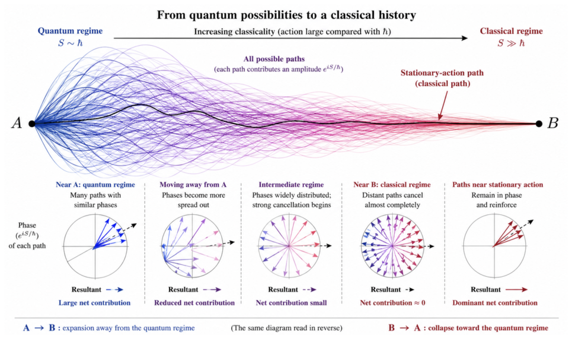
In a path-integral description (see Figure 2):
classical behaviour emerges in the semiclassical limit because destructive interference suppresses contributions far from stationary-action histories [15,16]. Near the high-density state, however, the semiclassical approximation itself may cease to be adequate: the path integral need no longer be dominated by a narrow neighbourhood of a single classical trajectory, and a broader set of quantum configurations may contribute to the evolution [17].
The approach to the bounce can therefore be summarized schematically as
This is the reverse of the transition usually emphasized in early-Universe cosmology. Standard inflationary calculations begin with quantum fluctuations and ask how they become classical perturbations. In a bouncing cosmology there is also a preceding process: initially classical structures and fields are driven by gravitational collapse toward an increasingly quantum state.
Figure 2.
How a classical history emerges from quantum possibilities. In Feynman’s formulation of quantum mechanics, every possible path between A and B contributes an amplitude. When the characteristic action is comparable to ℏ (left), many alternatives can contribute significantly. As the action becomes large compared with ℏ, the phases of paths far from stationary action vary rapidly and their contributions increasingly cancel. Paths close to the stationary-action trajectory remain approximately in phase and reinforce one another, so a single classical history comes to dominate (right). The fading paths represent destructive interference, not possibilities that have ceased to exist. Later we will encounter the same transition in reverse, when classical gravitational collapse approaches a regime where quantum alternatives can no longer be ignored.
Figure 2.
How a classical history emerges from quantum possibilities. In Feynman’s formulation of quantum mechanics, every possible path between A and B contributes an amplitude. When the characteristic action is comparable to ℏ (left), many alternatives can contribute significantly. As the action becomes large compared with ℏ, the phases of paths far from stationary action vary rapidly and their contributions increasingly cancel. Paths close to the stationary-action trajectory remain approximately in phase and reinforce one another, so a single classical history comes to dominate (right). The fading paths represent destructive interference, not possibilities that have ceased to exist. Later we will encounter the same transition in reverse, when classical gravitational collapse approaches a regime where quantum alternatives can no longer be ignored.
3.4. From the Quantum State Back to a Classical Universe
After the turning point, the process reverses. Expansion reduces the density, weakens interactions and increases the separation between the relevant degrees of freedom. The quantum high-density state evolves into perturbations of the expanding background, which subsequently decohere and become effectively classical.
The complete sequence is therefore
The first transition is driven by collapse, increasing density and growing correlations. The second is driven by expansion, dilution and decoherence. The bounce sits between them as the regime in which the classical spacetime description is least adequate.
This viewpoint also changes the interpretation of the origin of primordial structure. Quantum fluctuations need not emerge from an otherwise structureless beginning. The quantum state at the bounce may contain information inherited from the contracting phase together with fluctuations generated by the high-curvature dynamics itself. During expansion these quantum fluctuations are converted into the classical matter and metric perturbations from which the observed cosmic web eventually develops.
The details of this conversion depend on the microscopic theory. A particular quantum-gravity model must specify the degrees of freedom present at the bounce, their quantum state, their characteristic scale and their subsequent evolution. It may also determine whether discrete symmetries such as PT are preserved or broken during the emergence of the expanding branch.
3.5. Deflation, Inflation and the Meaning of Curvature
Constancy of the FLRW curvature parameter k is a property of the background ansatz, not a distinctive prediction of a bounce.
The semiclassical bounce does more than replace the singularity by a smooth transition. If the high-density state approaches a quasi-de Sitter configuration with , then the same dynamics that produces accelerated expansion after the bounce also implies an approximately time-reversed accelerated contraction before it. The contracting branch can therefore contain a period of deflation, followed by an inflationary phase after the bounce.
This changes the usual interpretation of inflation [18]. In standard cosmology, inflation is often invoked to explain the observed smallness of spatial curvature because the curvature contribution to the Friedmann equation, , is rapidly diluted as the scale factor grows. Equivalently, is driven toward zero during a sufficiently long period of accelerated expansion. For an initial contracting epoch i with , define and . Then
The expansion from the end of inflation to today depends on reheating and the subsequent thermal history.
In a bouncing cosmology, however, the pre-bounce evolution contains the opposite process. During deflation the scale factor decreases and the physical curvature contribution grows. To first approximation, a sufficiently symmetric inflationary phase after the bounce reverses the preceding deflationary evolution. The comoving curvature constant k itself is unchanged throughout the process: what changes is the physical curvature scale through its dependence on a.
The interpretation of the observed small curvature is therefore different. Post-bounce inflation need not be responsible for creating an exceptionally flat Universe from generic initial conditions. Instead, the combination of deflation and inflation can approximately restore the curvature scale inherited from the original finite perturbation. The present value of the curvature can then retain information about the initial conditions of the collapsing region.
For a finite overdensity embedded in a larger background, a small positive curvature corresponds to a perturbation that was very large in spatial extent but only weakly overdense. Such a perturbation can nevertheless become gravitationally bound and eventually collapse. In this sense, the observed near-flatness of the Universe need not imply that the underlying spatial curvature is exactly zero, nor that inflation has erased all memory of the initial state. A small residual curvature may instead be a fossil of the original perturbation from which the finite Universe formed.
This distinction is important because the inflationary phase is then assigned a different physical role. Its primary function is not to explain why the global curvature parameter is small, but to connect the high-density quantum state to the expanding semiclassical Universe and to generate the nearly scale-invariant spectrum of primordial fluctuations. The amount of residual curvature becomes an independent observable that probes the large-scale initial conditions of the collapse.
3.6. Two Origins of Primordial Structure
A bouncing cosmology also changes the interpretation of the origin of cosmic structure. In standard inflationary cosmology, essentially all primordial inhomogeneities are assumed to originate from quantum fluctuations generated during inflation and subsequently stretched beyond the Hubble radius [18]. These fluctuations are nearly Gaussian and nearly scale invariant, providing the initial conditions from which the observed large-scale structure develops.
In a finite Universe with a preceding contracting phase, there can be an additional source of structure [14]. Gravitational instability operates during contraction just as it does during expansion, and sufficiently overdense regions can collapse, virialize or form compact objects before the background reaches the high-density state. As the magnitude of the Hubble parameter grows during contraction, the apparent horizon shrinks. Structures whose physical size becomes larger than therefore pass outside causal contact with the surrounding medium.
Once this occurs, their internal evolution becomes effectively decoupled from the large-scale background. These pre-existing nonlinear perturbations can survive the approach to the bounce as super-horizon relics and re-enter the causal horizon during the subsequent expansion. The expanding Universe can therefore contain two physically distinct contributions to its primordial density field,
where denotes the approximately Gaussian, nearly scale-invariant fluctuations generated during inflation, while represents nonlinear structures inherited from the contracting phase.
The two components need not have the same statistical properties or physical origin. Inflationary fluctuations naturally dominate the smooth primordial spectrum measured in the CMB and the large-scale matter distribution. Relic perturbations can instead be rare, highly nonlinear and strongly non-Gaussian, contributing primarily on the scales associated with compact objects, early halos or black-hole seeds.
This separation is particularly relevant for the formation of primordial compact objects. In conventional scenarios, producing a significant abundance of primordial black holes from the same nearly Gaussian fluctuation field measured in the CMB generally requires access to the extreme tail of the distribution, or a substantial enhancement and often non-Gaussian modification of the primordial spectrum on smaller scales. In the present framework this requirement is relaxed because the compact-object seeds need not originate from exceptionally large inflationary fluctuations.
Virialized structures formed during contraction can already possess overdensities far above the threshold required for black-hole collapse when they later re-enter the horizon. Their existence is therefore compatible with an inflationary fluctuation field that remains close to Gaussian and nearly scale invariant. The two observational requirements,
can be satisfied by two different populations rather than by forcing a single primordial spectrum to account for both.
This provides a natural way of combining the conventional successes of inflationary structure formation with genuinely pre-bounce relics. The inflationary component seeds the large-scale cosmic web, while the relic component may contribute to dark matter, provide early seeds for supermassive black holes and generate distinctive gravitational-wave or lensing signatures. Their relative abundance and characteristic mass scale depend on the high-density parameter and on the duration of the contracting and inflationary phases, providing another route by which observations can constrain the physics of the bounce.
3.7. A Bounce Without Committing to a Unique Quantum Theory
It is useful to keep the logical ingredients distinct. The finite BHU geometry supplies the global conditions for collapse and positive curvature. The assumption of a finite-density quantum state replaces the singular endpoint. Together these ingredients allow a nonsingular bounce. They do not by themselves identify the microscopic theory responsible for that state.
This distinction allows the BHU to be used as a framework in which different theories of quantum gravity can be tested. A candidate theory should ideally predict quantities such as
together with the spectrum and symmetry properties of the perturbations emerging from it.
An equally important requirement is stability. The existence of a regular homogeneous solution does not by itself guarantee that the bounce is robust against anisotropic or inhomogeneous perturbations. In classical contraction, shear contributions generally grow rapidly, with an effective energy density scaling as , and the associated anisotropy problem has been studied extensively in nonsingular and contracting cosmologies [19,20]. Vector perturbations can also grow during contraction in specific bouncing scenarios [21,22]. The post-bounce de Sitter-like expansion is driven towards isotropy by the usual cosmic no-hair mechanism, but this argument does not apply in the same way to the contracting branch. Whether anisotropies and other perturbations remain perturbative until the finite-density state is reached therefore constitutes an additional consistency condition on the model.
This should be regarded not merely as a limitation but as a potential falsifiability criterion. A viable quantum completion must either show that the growth of anisotropy and inhomogeneous perturbations remains sufficiently small throughout the finite contraction, or provide a high-density mechanism that modifies their classical evolution before they backreact strongly on the background. Related stability problems and no-go results are known in particular Galileon and Horndeski nonsingular constructions [23,24], while modified-gravity models provide examples in which some of these difficulties can be altered or avoided [25,26,27]. These results do not apply directly to the positively curved ground-state bounce considered here, but they illustrate why stability must ultimately be established for the specific quantum-gravity completion. Quantum coherence across the bounce could in principle play such a role, but no explicit mechanism is assumed here.
These predictions can then be confronted with independent observations. In the following sections we use quadratic gravity as a concrete example because its sector provides a well-defined high-curvature inflationary dynamics whose normalization is already constrained by the CMB. We will also consider PT-symmetric quantum descriptions as possible realizations of the quantum state across the bounce. Neither construction is required by the finite-universe argument itself. Their value is that they turn the otherwise unspecified high-density state into a predictive physical model whose viability can be tested not only through its observable relics, but also through the dynamical stability of the bounce itself.
4. Quantum Gravity in a Finite Bouncing Cosmology
The finite-universe construction described above does not by itself determine the microscopic physics of the bounce. General Relativity provides the global gravitational evolution through most of the contracting and expanding phases, but as the density and curvature approach the scale , the classical description must eventually be replaced by a quantum one. The role of a quantum-gravity completion is therefore not to create the finite cosmological setting, but to determine what happens at its high-density endpoint.
This distinction is useful because it separates two logically different questions. The first is global and essentially classical: can a finite gravitating region collapse, reach a minimum size and subsequently re-expand? The second is microscopic: what quantum dynamics regulates the high-curvature state, prevents a singularity and determines the perturbations and particle content emerging from the bounce?
A successful quantum-gravity completion of a finite bouncing cosmology should ideally address several requirements simultaneously. It should recover General Relativity at low curvature, provide a consistent quantum description at high curvature, preserve unitarity, regulate or remove classical singularities and produce a semiclassical expanding state compatible with observations. In addition, if the theory is to be empirically useful, it should determine at least some of the characteristic scales and symmetry properties of the bounce rather than leaving them as arbitrary initial conditions.
In the present framework, particularly important quantities include
together with the duration of the high-density phase, the primordial fluctuation spectrum and the symmetry properties of the quantum state. These quantities control very different observables: the amplitude and scale dependence of CMB perturbations, the survival of pre-bounce relics, the minimum horizon scale, possible matter–antimatter asymmetries and strong-gravity signatures.
The finite bouncing Universe therefore provides an unusual setting in which a quantum-gravity theory can potentially be tested indirectly over a very wide range of scales. The microscopic dynamics near the bounce may influence observables that later appear in the CMB, large-scale structure, relic compact objects or gravitational waves. Different quantum-gravity completions need not make the same predictions for these quantities, allowing the cosmological setting itself to act as a discriminator between them.
4.1. What Should a Quantum-Gravity Completion Explain?
At the most basic level, the classical singularity must be replaced by a physically admissible quantum state. This does not necessarily require that curvature vanish or that the bounce be completely classical. It requires instead that physical observables remain finite and that the evolution connect the contracting and expanding semiclassical phases without loss of probability or predictive power.
A useful way of organizing the required physics is
The quantum theory should then answer four related questions.
First, what sets the limiting density ? In a phenomenological bounce this quantity can simply be introduced as a new scale. A more predictive theory should relate it to fundamental couplings or dynamically generated scales.
Second, what determines the duration and geometry of the bounce? This controls the minimum causal radius and therefore which structures remain sub-horizon and which become frozen relic perturbations.
Third, what quantum state emerges into the expanding branch? The answer determines the primordial scalar and tensor perturbations, their parity properties and their correlations.
Finally, how does the quantum state convert into ordinary matter and radiation? The reheating or quantum-to-classical transition is where the gravitational degrees of freedom become the particle content of the hot Big Bang, and it may also be where primordial symmetry breaking is transferred to matter.
These questions are closely related but need not have the same microscopic origin. Matter degeneracy can regulate compression, higher-curvature terms can dominate the gravitational action, discrete spacetime symmetries can determine the structure of the quantum state and particle interactions can control reheating. A complete theory should explain how these ingredients fit together.
4.2. Quadratic Gravity as a Worked Example
Quadratic gravity provides a particularly useful example because it extends General Relativity by the leading local curvature-squared operators and becomes increasingly relevant in the high-curvature regime [3,28]. In four dimensions the action may be written as
where is the reduced Planck mass, is the Weyl tensor and and are dimensionless couplings.
Interestingly, the sensitivity of cosmological predictions to higher-order terms in the gravitational effective action was already apparent in early studies of the quantum probability distribution of the cosmological constant [12].
The importance of the quadratic terms is twofold. First, they improve the ultraviolet behaviour of the gravitational propagator. Schematically,
making the theory perturbatively renormalizable. Second, the additional curvature terms introduce new dynamical sectors that become relevant precisely where classical General Relativity predicts large or divergent curvature.
The term introduces a scalar degree of freedom, the scalaron, whose characteristic mass is
In a homogeneous and isotropic FLRW background the Weyl tensor vanishes,
so the background high-curvature dynamics is governed primarily by the Ricci and sectors. The same scalaron dynamics that regulates the high-curvature evolution naturally generates the quasi-de Sitter phase of Starobinsky inflation.
Quadratic gravity is therefore particularly well suited to the finite-bounce picture. The contracting Universe can approach a high-curvature quasi-de Sitter state, pass through a nonsingular transition and emerge into an inflationary expanding phase. To first approximation, the high-density evolution possesses the qualitative structure already anticipated from the semiclassical bounce: deflation during contraction followed by inflation during expansion.
The significance of this example is that the relevant inflationary scale is not arbitrary. The observed amplitude of primordial scalar perturbations fixes to be of order
as discussed in detail below. Consequently, the same CMB measurement that determines the amplitude of primordial structure also fixes the characteristic scalaron mass and high-curvature scale of the theory.
This raises an important possibility for the BHU framework: the density of the semiclassical state may ultimately be related to the inflationary scale determined by . If this identification can be established, the bounce density would no longer be an independent parameter. It could instead be predicted by a coupling already measured through the primordial fluctuation spectrum.
At present this relation should be regarded as a hypothesis rather than an established result. The high-density state of the BHU has been motivated from many-body quantum degeneracy, whereas the quasi-de Sitter state of quadratic gravity follows from curvature dynamics. Demonstrating that the two descriptions correspond to the same physical state requires a microscopic treatment of matter and gravity together. Nevertheless, their shared properties—finite density, quasi-de Sitter evolution and a natural transition between contraction and expansion—make the comparison particularly suggestive.
4.3. The Role of the Weyl Sector
The Weyl-squared term does not affect an exactly homogeneous FLRW background, but it becomes important for departures from homogeneity and isotropy. It therefore controls aspects of the physics that are directly relevant to perturbations, tensor modes and strong-gravity environments.
In conventional quadratic gravity the additional spin–2 degree of freedom associated with the Weyl term leads to the well-known ghost problem. Recent formulations [29] have proposed alternative quantizations in which this sector is not interpreted as a propagating negative-norm particle. Direct-sum quantization provides one explicit example, in which the additional spin–2 mode is described through complementary PT-related sectors and does not belong to the physical asymptotic particle spectrum.
For the present review, the detailed implementation is secondary. The important point is that any viable quadratic quantum-gravity model must preserve the ultraviolet improvement provided by the Weyl sector while maintaining a positive and unitary physical state space. Different resolutions of the spin–2 problem may lead to different observable consequences for tensor perturbations, black-hole ringdown or horizon dynamics.
This is precisely where the finite-universe approach becomes useful. The microscopic treatment of the Weyl sector is not merely a formal issue at inaccessible energies: it can potentially influence primordial gravitational waves, parity-dependent tensor modes, quasinormal modes and extreme-mass-ratio inspirals.
4.4. Singularity Avoidance and the Finite-Action Criterion
Quadratic curvature terms also modify the status of singular gravitational histories. Near a classical singularity, quantities such as or can grow rapidly, causing the gravitational action to diverge. In a path-integral description,
histories with arbitrarily large action acquire rapidly oscillating phases and may be strongly suppressed relative to smoother configurations.
This motivates the finite-action criterion: physically relevant histories should possess a finite gravitational action. In higher-curvature gravity, this requirement can disfavor classes of singular and strongly anisotropic solutions and favour regular high-curvature configurations.
The finite-action argument alone does not uniquely determine the bounce. It constrains which histories can contribute significantly to the quantum evolution, while the global closed geometry and the matter state determine whether contraction actually reverses into expansion. In the BHU construction, these ingredients are complementary:
A successful microscopic theory should ultimately explain all three within a single framework.
4.5. From Microscopic Theory to Observable Parameters
The most important reason for embedding quantum gravity in a finite cosmology is that the fundamental parameters of the microscopic theory can become connected to measurable quantities.
For quadratic gravity, the schematic chain is
If the same dynamics determines , this extends to
The same microscopic theory can independently affect tensor perturbations and strong-gravity observables through its additional gravitational degrees of freedom. Thus a single quantum-gravity model may be constrained simultaneously by the CMB, the bounce scale, the relic population and black-hole gravitational-wave observations.
This is the central methodological point of the present paper. Quadratic gravity is useful not because it must be the unique theory describing the bounce, but because it illustrates how a concrete quantum-gravity completion can transform an otherwise phenomenological high-density state into a network of quantitative predictions. Other microscopic theories can be embedded in the same finite cosmological setting and confronted with the same observational programme.
The next step is to examine a more general property that may be required of the primordial quantum state: its behaviour under parity and time reversal. There are several independent reasons to take this symmetry seriously before considering how it may be broken. In quadratic gravity, the additional spin–2 sector that appears as a ghost in conventional quantization suggests that the usual single-sector description may be incomplete, while PT-related formulations provide one possible route to a unitary interpretation. In black-hole physics, the information-loss problem and the global structure of Einstein–Rosen geometries similarly point toward complementary descriptions associated with different causal regions or time orientations. Related ideas have appeared in different forms in the work of Einstein and Rosen, Schrödinger, ’t Hooft and others, long before their recent formulation in direct-sum quantum theory [30]. Strong-gravity observations may provide an additional test: the approximate isospectrality of axial and polar black-hole quasinormal modes reflects a deep symmetry of the underlying perturbation equations, and departures from this structure could reveal how such symmetries are modified by quantum gravity.
These considerations motivate treating PT symmetry not as a phenomenological assumption introduced to explain a particular observation, but as a possible organizing principle of the underlying quantum theory. Direct-sum quantization provides one explicit realization, but it is not unique and will be used here primarily as a worked example. If the fundamental high-density state is PT symmetric while the observed expanding semiclassical branch selects one orientation, PT symmetry must then be broken during the quantum-to-classical transition. Such symmetry breaking can leave measurable imprints in the primordial perturbations and, through CPT invariance, may also be connected to the particle–antiparticle asymmetry of the Universe.
5. PT Completion and the Primordial Quantum State
The discussion so far has focused on the geometry and dynamics of a finite bouncing Universe. We now turn to a different question: what symmetry should characterize the quantum state that connects the contracting and expanding branches?
A natural possibility is that the fundamental quantum description is invariant under the combined action of parity and time reversal, PT, even if the semiclassical Universe observed on one side of the bounce is not. In this picture, PT symmetry belongs to the underlying quantum state or evolution law, while the emergence of a particular expanding branch corresponds to a spontaneous or effective breaking of that symmetry.
This distinction is important. If PT asymmetry were introduced only at the phenomenological level, it would amount to adding a new ingredient in order to explain an observational anomaly. If PT symmetry instead follows from deeper requirements of quantum gravity, such as unitarity, complementarity or the consistent treatment of apparently ghost-like sectors [29], then any observed PT breaking becomes a probe of how the fundamental quantum state gives rise to the classical Universe.
5.1. PT Symmetry as an Organizing Principle
In ordinary quantum mechanics, parity reverses spatial orientation,
while time reversal reverses the direction of time,
and acts antiunitarily on the quantum state. Their combined action relates configurations with opposite spatial and temporal orientation.
For quantum gravity this possibility is especially suggestive. Horizons divide spacetime into regions that need not admit a single global time orientation accessible to one observer. Black-hole interiors, Einstein–Rosen bridges and cosmological bounces naturally introduce pairs of causally or temporally complementary regions. A quantum description that treats one orientation as fundamental while discarding the other can therefore obscure symmetries that are present in the full geometry. We will call this idea PT completion.
The idea that a complete quantum description may require complementary sectors has appeared in several forms. Einstein and Rosen [31] introduced bridge geometries connecting apparently distinct spacetime regions; Schrödinger [32] emphasized the nonlocal and relational character of entangled quantum states; and more recent approaches, including antipodal constructions and horizon-based descriptions [33], have stressed that information associated with different causal regions may belong to a single global quantum state. Direct-sum quantum theory provides one explicit modern realization in which opposite PT orientations are incorporated from the outset [30].
The common motivation is not that all these constructions are equivalent, but that quantum gravity may require a description more global than the semiclassical viewpoint available to a single observer.
5.2. Direct-Sum Quantization as One Realization
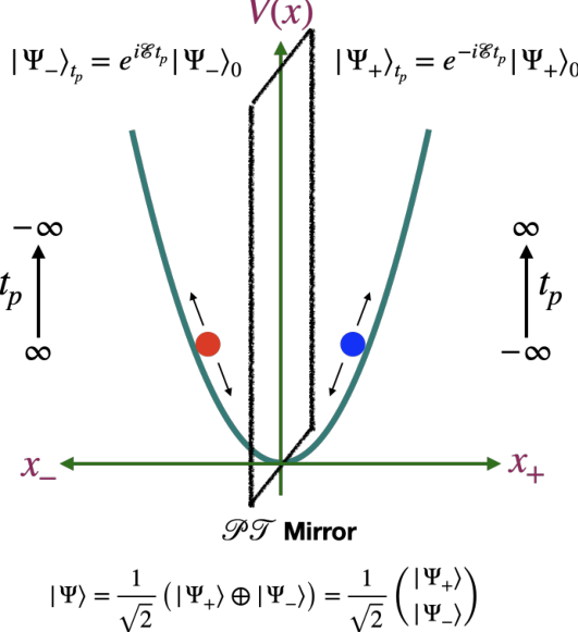
In direct-sum quantum theory, the Hilbert space is decomposed into two complementary sectors,
which are related by PT transformation. The quantum state can be represented schematically as
with the two components evolving with opposite microscopic time orientations.
The corresponding evolution operator takes a block-diagonal form,
so that the complete state evolves unitarily even though the two sectors carry opposite time orientation.
In this framework, the contracting and expanding sides of a bounce can be interpreted as semiclassical manifestations of the two complementary sectors. The full quantum state can preserve PT symmetry even though an observer inhabiting one branch experiences a definite arrow of time.
This construction is useful because it illustrates explicitly how a PT-symmetric fundamental state can coexist with a PT-asymmetric observable Universe. It should not, however, be regarded as the unique realization of this idea. The observational arguments developed below require only that the primordial quantum state possess an approximate PT symmetry and that the emergence of the expanding branch permits this symmetry to be broken.
Figure 3.
The picture depicts the new understanding of quantum harmonic oscillator in a direct-sum Hilbert space. Time is a parameter in quantum theory. In contrast, the spatial position is an operator. A quantum state here is described by a direct-sum of two components in parity conjugate points in physical space.
Figure 3.
The picture depicts the new understanding of quantum harmonic oscillator in a direct-sum Hilbert space. Time is a parameter in quantum theory. In contrast, the spatial position is an operator. A quantum state here is described by a direct-sum of two components in parity conjugate points in physical space.
5.3. Symmetry Breaking at the Quantum–Classical Transition
Suppose that the high-density state at the bounce is PT symmetric. The two semiclassical branches can then be represented schematically as
The full quantum state may contain both orientations symmetrically, while the classical Universe accessible to us corresponds to one branch.
The emergence of a definite branch therefore resembles semiclassical branch selection. The underlying equations and quantum state can preserve PT, but the realized semiclassical history does not.
We may parameterize the departure from exact PT symmetry by a dimensionless amplitude,
with non-zero characterizing the asymmetry of the selected branch.
The precise microscopic definition of depends on the theory. It may correspond to an imbalance between PT-related sectors, a relative phase, an asymmetry in the primordial two-point function or a difference in the occupation of parity-related modes. For the observational discussion it is useful to treat as an effective parameter characterizing the amount of primordial PT breaking that is transferred to cosmological perturbations.
5.4. A Possible Resolution of the Past Hypothesis and Quantum-Information Problems?
A long-standing difficulty in cosmology is the origin of the thermodynamic arrow of time. The microscopic laws are to a very good approximation invariant under time reversal, yet the observed Universe displays a pronounced temporal asymmetry: entropy increases, records accumulate and gravitational structure grows in one direction of time. The conventional resolution is the Past Hypothesis: the Universe is assumed to have emerged from an extraordinarily special low-entropy state. In cosmology this problem is particularly acute because the early Universe was remarkably smooth. Matter and radiation could already be close to thermal equilibrium while the gravitational degrees of freedom were very far from their high-entropy, strongly clustered state.
A bouncing cosmology appears at first to make this problem harder. A contracting classical Universe would not generically approach the bounce smooth and empty. Gravitational instability can produce structure and black holes, while compression drives the material sector towards an increasingly hot radiation-dominated state. The contracting branch can therefore carry a substantial amount of both thermodynamic and gravitational information into the high-density regime. If the expanding branch begins instead in the smooth state inferred from the CMB, one must explain what has happened to that information and why entropy appears to grow away from the bounce on our side.
PT completion suggests a different way of posing the problem. The bounce need not be treated as an ordinary classical state through which a single thermodynamic history must pass continuously. Near the transition the semiclassical description itself breaks down and is replaced by the complete quantum state. If that state contains two PT-related sectors with opposite microscopic time orientations, then the two classical branches emerging from it can possess thermodynamic arrows directed away from the quantum regime,
where and denote the physical time orientations experienced within the two semiclassical branches. No entropy decrease along either observer’s classical arrow is required, and no classical entropy function need be assumed to evolve smoothly through the quantum transition itself.
In this interpretation the apparent low entropy of the expanding branch is not necessarily a fundamental boundary condition imposed at an absolute beginning. It may instead characterize the classical state that becomes accessible when the quantum system projects onto one semiclassical sector. The relevant distinction is therefore between the information contained in the complete quantum state and the information accessible within a particular classical branch.
This distinction also changes the quantum-information problem. If the evolution of the complete state
is unitary, information need not be destroyed at the bounce simply because it is absent from the classical observables available on the expanding side. Information carried by the contracting branch may remain encoded in the full PT-complete state or in correlations that are inaccessible to an observer restricted to one semiclassical sector. What appears classically as information loss can then represent a loss of accessibility, rather than a failure of unitary quantum evolution.
This viewpoint has a close conceptual parallel in the ER=EPR conjecture of Maldacena and Susskind [34]. In that proposal, two entangled black holes that appear as distinct systems from the semiclassical viewpoint may be connected through an Einstein–Rosen bridge or wormhole, suggesting that geometrical separation and quantum separation need not coincide. The bridge is not a traversable channel through which classical information can simply be recovered; rather, it provides a geometrical representation of correlations belonging to the complete quantum state. PT completion invokes a related principle in a cosmological setting: the contracting and expanding semiclassical sectors may appear causally and temporally distinct while remaining components of a single quantum description. Information inaccessible within one branch need therefore not be absent from the complete state.
ER=EPR provides a particularly concrete example of a more general lesson: horizons and causal separation can limit classical accessibility without implying a corresponding factorisation of the underlying quantum state. ER=EPR suggests that quantum entanglement can connect what classical geometry regards as separate regions of space. PT completion raises the analogous possibility that a complete quantum state can connect what semiclassical cosmology regards as opposite orientations of time.
This observation is closely analogous to the role of horizons in quantum gravity. A causal horizon restricts the information accessible to a particular observer without necessarily implying that the complete quantum state has lost that information. In the same way, the quantum–classical transition at the bounce can erase or strongly suppress the detailed classical imprint of the contracting branch while preserving the information in the complete quantum description. The smooth expanding state need not therefore imply that the pre-bounce history never existed.
PT completion does not by itself constitute a complete derivation of the Past Hypothesis. In particular, a microscopic theory must still explain why the semiclassical state emerging on either side has the observed low gravitational complexity and how the relevant classical coarse graining arises. The proposal is instead that the low-entropy initial condition and the information problem need not be independent assumptions. Both may originate from the same quantum-to-classical transition: a PT-symmetric complete state can preserve information globally while producing classical branches whose entropy and records grow away from the transition.
This possibility also provides a direct link to observation. If the quantum state were exactly PT symmetric and the emergence of the two branches preserved that symmetry perfectly, no preferred PT orientation would remain in primordial fluctuations. A small asymmetry in the quantum–classical transition, characterized phenomenologically by , can instead leave a fossil of this branch selection in the statistics of the primordial perturbations. Because the spatial part of PT acts through parity, one of the cleanest places to search for such a fossil is the large-scale parity structure of the cosmic microwave background.
5.5. Parity in the Primordial Perturbations
For a scalar temperature field , parity acts as . A particular field configuration satisfying has only even multipoles; a configuration satisfying has only odd multipoles. In either case the power in the opposite parity sector vanishes. Every map can be decomposed into these two eigencomponents,
Their relative power quantifies antipodal symmetry of the observed configuration.
This statement differs from parity invariance of an ensemble. A zero-mean isotropic Gaussian scalar ensemble has covariance
Under parity it acquires a factor , which is unity on the diagonal. The covariance, and therefore this Gaussian ensemble, is parity invariant for any non-negative , including an even–odd modulation.
The cosmic microwave background (CMB) provides a particularly direct probe of such local parity on the largest observable scales (see Figure 4).
In standard inflation, the primordial spectrum is assumed to be parity symmetric, so the ensemble prediction contains no systematic preference for even or odd multipoles. Direct-sum inflation (DSI), by contrast, predicts a scale-dependent parity asymmetry on the largest scales as a consequence of the PT structure of the primordial quantum state. The effect is not fitted phenomenologically to the observed CMB: the parity modulation follows from the theory without introducing an additional free parameter [36].
A convenient statistic is the ratio of even- to odd-parity power,
where and denote suitably averaged even- and odd-multipole powers. Exact parity balance corresponds statistically to
Planck temperature maps instead show a persistent preference for odd parity on the largest angular scales, corresponding to an asymmetry of order . The DSI prediction lies close to the observed value, whereas the standard inflationary prediction is centered on parity balance.
The statistical interpretation of this result is important. Large-scale CMB anomalies are often described as being limited by cosmic variance because only a small number of independent modes are available at low multipoles. This is correct when asking how unusual a particular realization is within a fixed cosmological model, but it is not the same question as comparing two models that predict different probability distributions for the same observables.
In Bayesian model comparison one considers
where and denote the competing primordial models. Cosmic variance is already incorporated in the likelihoods predicted by each model. It broadens the expected distributions, but it does not erase the information contained in the fact that the observed realization may lie systematically closer to one distribution than to the other.
Using Monte Carlo realizations of the Planck temperature sky, the low-multipole power spectrum gives a cumulative Bayes factor of approximately
by , while the quadrupole alone gives . More significantly, the joint distribution of the quadrupole amplitude , the even-to-odd parity ratio and the antipodal correlation gives
in favour of the parity-asymmetric DSI prediction over standard inflation.
The key point is therefore not that cosmic variance is absent, but that it is explicitly included in the comparison. Cosmic variance limits how precisely the underlying low-multipole spectrum can be reconstructed from a single sky, but it does not prevent Bayesian discrimination between models that predict different statistical distributions for that sky. For the combined parity-sensitive statistics considered here, the observed CMB is several hundred times more probable under the DSI prediction than under standard parity-symmetric inflation.
The angular correlation function provides an equivalent real-space description,
At antipodal separation,
even and odd multipoles contribute with opposite signs. The observed suppression and negative character of the large-angle antipodal correlation are therefore closely connected to the same odd-parity preference and contribute independently to the Bayesian evidence.
5.6. From CMB Parity to a PT-Breaking Amplitude
The observed parity imbalance can be expressed phenomenologically as an effective amplitude of primordial PT breaking. Schematically,
where the precise numerical definition depends on the multipole weighting and estimator adopted.
The large-scale CMB measurements indicate an asymmetry of order
This is also the characteristic magnitude of the low-multipole parity modulation predicted in the direct-sum construction. The effect decreases toward smaller angular scales, where the standard approximately parity-symmetric primordial spectrum is recovered.
Within this framework, should therefore be regarded as an observationally inferred parameter rather than merely as a qualitative characterization of a CMB anomaly. The evidence is not based only on the measured odd-parity excess itself. The same model simultaneously provides a better description of the low quadrupole, the even–odd power ratio and the antipodal correlation, with the joint analysis yielding
Thus the data favour the PT-asymmetric prediction over the parity-symmetric standard-inflation prediction by posterior odds of order several hundred to one, assuming comparable prior probabilities for the two models.
This distinction is important. The large cosmic variance of the lowest multipoles does not make statistically meaningless. Rather, it is part of the predicted distribution against which the observation is compared. Within the primordial PT framework, the CMB therefore provides statistically significant evidence for a non-zero effective symmetry-breaking amplitude, with a preferred value of order
What remains model dependent is the physical interpretation of this measured asymmetry. Identifying with symmetry breaking in the primordial quantum state assumes that the observed parity structure is cosmological and that the theoretical mapping between the underlying PT sectors and the CMB is correct. Foreground residuals, masks and estimator choices must therefore continue to be tested. However, these possible systematics should be distinguished from cosmic variance: the latter is already included in the likelihood calculation and does not account for the preference of one model over the other.
The next requirement is independent confirmation. If the inferred is genuinely primordial, the same symmetry breaking should leave correlated signatures in other parity-sensitive observables, particularly CMB polarization and the primordial tensor sector. These provide genuine falsification tests of the interpretation rather than merely additional ways of increasing the statistical significance of the temperature result.
Figure 5.
Joint distribution of three statistics characterizing the large-scale CMB parity asymmetry: the quadrupole amplitude , the temperature parity ratio , and antipodal correlation . Grey contours and one-dimensional distributions show the probability density obtained from Monte Carlo realizations of the observed sky. Red markers indicate the mean predictions of the SI model, while blue markers show the DSI prediction. The coloured dashed lines correspond to measurements from the four Planck component-separated maps (Commander, SMICA, SEVEM and NILC [37]), illustrating that the differences between foreground-cleaning methods are much smaller than the intrinsic cosmic variance. The observed realization lies much closer to the DSI prediction than to the SI expectation, giving a join Bayes factor in favour of DSI.
Figure 5.
Joint distribution of three statistics characterizing the large-scale CMB parity asymmetry: the quadrupole amplitude , the temperature parity ratio , and antipodal correlation . Grey contours and one-dimensional distributions show the probability density obtained from Monte Carlo realizations of the observed sky. Red markers indicate the mean predictions of the SI model, while blue markers show the DSI prediction. The coloured dashed lines correspond to measurements from the four Planck component-separated maps (Commander, SMICA, SEVEM and NILC [37]), illustrating that the differences between foreground-cleaning methods are much smaller than the intrinsic cosmic variance. The observed realization lies much closer to the DSI prediction than to the SI expectation, giving a join Bayes factor in favour of DSI.
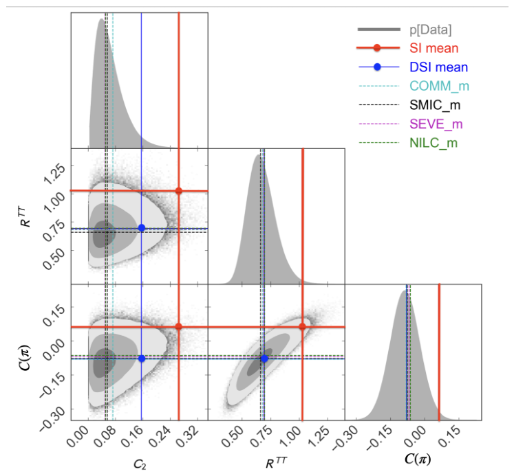
5.7. Beyond Temperature: Polarization and Tensor Modes
If the parity asymmetry is primordial, it should not be confined to the temperature map. The same underlying state should leave correlated signatures in CMB polarization and potentially in primordial gravitational waves.
Temperature and E-mode polarization are parity even, while B-mode polarization is parity odd. Cross-correlations such as and , which vanish in a parity-symmetric ensemble under standard assumptions, provide particularly sensitive tests of primordial parity violation.
A genuine PT-breaking mechanism should therefore predict a consistent pattern across
rather than explaining only one statistic in the temperature sky.
The tensor sector provides an additional test. A PT-asymmetric primordial state may produce unequal amplitudes for opposite tensor helicities,
leading to chiral primordial gravitational waves. Such a signal could appear in CMB polarization or, depending on the energy scale and transfer function, in future direct gravitational-wave observations.
The decisive test is therefore not the existence of one parity anomaly but cross-consistency among several independent parity-sensitive observables.
5.8. PT, CPT and the Origin of Matter
The possibility of primordial PT breaking has another potentially important consequence. Relativistic quantum field theory is expected to preserve CPT under broad conditions. If CPT remains exact at the fundamental level while the observed cosmological branch breaks PT, then the corresponding state must also distinguish charge conjugation.
Schematically,
Thus a PT-asymmetric branch of an underlying CPT-symmetric theory may also be C asymmetric.
This observation does not by itself generate a baryon asymmetry. Charge-conjugation breaking is not sufficient if baryon and lepton numbers are exactly conserved. Actual baryogenesis requires processes that change B or L, together with the appropriate departure from equilibrium or equivalent dynamical conditions.
Nevertheless, primordial PT breaking can provide the symmetry bias that such processes require. During reheating, when the high-density gravitational state is converted into matter and radiation, the same asymmetry measured through the primordial perturbations may be transferred to particle populations. If baryon- or lepton-number-violating interactions are active, a PT-related asymmetry can then seed a non-zero abundance, which electroweak sphalerons subsequently redistribute between baryons and leptons.
This possibility is especially intriguing because it connects two apparently unrelated observations: the parity structure of the CMB and the matter–antimatter asymmetry of the Universe.
5.9. An Observational Symmetry Parameter
The broader significance of is therefore similar to that of discussed previously. Both quantities characterize microscopic properties of the high-density phase, but both may be inferred indirectly from late-time observations.
The emerging chain is
This turns discrete symmetry from a formal property of the quantum theory into an experimentally accessible parameter.
The next step is to connect this symmetry information with the dynamical scale of the high-curvature phase. Quadratic gravity provides a particularly useful example because the amplitude of scalar perturbations fixes the coupling , while the same scalaron dynamics controls inflation and reheating. The combination of and therefore opens the possibility of linking the CMB amplitude, primordial parity and the observed baryon abundance within a single consistency framework.
6. Inflation and Reheating in Quadratic Gravity
Quadratic gravity provides a particularly economical realization of the inflationary phase discussed above. In a homogeneous and isotropic background the Weyl tensor vanishes, so the background dynamics of
is governed by the Einstein–Hilbert and terms. The resulting theory is dynamically equivalent to General Relativity coupled to an additional scalar degree of freedom, the scalaron.
This is important for a finite bouncing cosmology because the same high-curvature sector that becomes relevant near the bounce naturally generates an approximately de Sitter phase. On the expanding branch this appears as Starobinsky inflation, while the time-reversed contracting branch contains a corresponding deflationary phase. Inflation is therefore not inserted independently into the cosmological history: it emerges from the high-curvature gravitational dynamics.
6.1. Gravity and the Scalaron
The sector can be written in the conventional form
where
After a conformal transformation to the Einstein frame, the additional gravitational degree of freedom is represented by a canonical scalar field with potential
At large the potential approaches a nearly constant plateau,
and the expansion becomes quasi-de Sitter. The scalaron therefore provides a purely gravitational mechanism for inflation without requiring the introduction of an additional fundamental inflaton field.
For a finite bouncing cosmology this same solution can be considered on both sides of the bounce. During contraction, the system approaches the high-curvature plateau through an approximately time-reversed quasi-de Sitter phase; after the turning point, it leaves the high-density state through inflationary expansion. To leading order the sequence is therefore
The detailed matching through the bounce depends on the microscopic quantum-gravity state and cannot be inferred from the classical solution alone. Nevertheless, the existence of the quasi-de Sitter attractor on the expanding branch makes quadratic gravity a natural realization of the semiclassical dynamics introduced in Sec. 3.
6.2. The CMB Amplitude Fixes the Quadratic Coupling
A particularly attractive feature of inflation is its predictivity. The scalar perturbation amplitude is
where the star denotes evaluation when the pivot scale exits the Hubble radius.
For Starobinsky inflation, at e-folds before the end of inflation,
which gives
The observed value [38]:
therefore determines
for –60.
Equivalently, the scalaron mass is fixed to be
or approximately
Thus the strength of the quadratic correction is not a free high-energy parameter once the primordial fluctuation amplitude is specified. A measurement made from CMB temperature and polarization fluctuations determines a coupling in the ultraviolet gravitational action.
The same model predicts, to leading order,
giving and for . The observed scalar spectrum therefore constrains not only the inflationary phenomenology but the scale of the underlying high-curvature gravitational dynamics.
6.3. Inflation as the Expanding Side of the Bounce
In the conventional interpretation, Starobinsky inflation is treated as the earliest dynamically specified stage of the Universe. In the finite bouncing picture it instead describes the expanding side of a more complete history.
As discussed previously, the quasi-de Sitter behaviour generated by the sector has an approximately time-reversed counterpart during contraction. The inflationary expansion therefore restores, to first approximation, the evolution undergone during the preceding deflationary phase.
This distinction is particularly relevant for spatial curvature. The curvature constant k does not change during either phase, while its physical contribution scales as
Deflation increases this contribution as the Universe contracts, and inflation subsequently suppresses it as the Universe expands.
Consequently, inflation need not be interpreted as the mechanism that determines why the global curvature of the finite Universe is small. If the contracting and expanding quasi-de Sitter phases are approximately symmetric, much of the flattening produced after the bounce simply reverses the curvature amplification produced before it. The residual curvature retains information about the original finite perturbation that underwent collapse.
This provides a conceptually different interpretation of near-flatness. A very large, weakly overdense perturbation can correspond to a small positive curvature from the outset. The present value of can then retain information about these initial conditions rather than being exponentially erased by an arbitrarily long period of one-sided inflation.
6.4. From Inflation to Reheating
Inflation ends when the scalaron leaves the flat part of the potential and begins to oscillate around its minimum. Near the minimum,
so the scalaron behaves approximately as a massive coherent field.
Its oscillations subsequently decay into ordinary quantum fields through gravitationally induced couplings. The energy stored in the high-curvature gravitational sector is thereby transferred to particles and radiation,
Reheating therefore has a particularly transparent interpretation in quadratic gravity: it is the process through which the additional gravitational degree of freedom created by the term transfers its energy to the particle sector.
In the bouncing picture, this is also part of the broader quantum-to-classical transition. The high-density state first gives rise to an expanding quasi-de Sitter geometry and quantum fluctuations. Scalaron decay then populates the Universe with particles, while the primordial perturbations decohere and become the classical density perturbations from which later structure forms.
The reheating stage is therefore potentially important for more than the thermal history. It is also the epoch during which symmetry properties inherited from the primordial quantum state may be transferred to the matter sector.
6.5. A Possible Connection Between and the Bounce Density
The fact that is fixed observationally raises a particularly interesting question. Can the same coupling also determine the characteristic density of the high-density state?
The plateau of the scalaron potential defines a natural energy density,
For , this corresponds to an energy scale
of the familiar inflationary order.
The associated Hubble scale is
This suggests the possible identification
Such a relation would be remarkable because it would connect the bounce density directly to the measured amplitude of primordial fluctuations:
Using Eq. (78),
so that
The characteristic bounce horizon would then also cease to be an arbitrary parameter:
It would ultimately be related to the CMB normalization through .
This identification is not yet established. The scalaron plateau energy is the energy density of a high-field quasi-de Sitter configuration, whereas was introduced as the density of the semiclassical quantum-supported state reached during gravitational collapse. In particular, the minimum of the scalaron potential has zero potential energy; should therefore not be interpreted as the ground-state energy density of the scalaron itself.
The question is instead whether the same high-curvature dynamics that produces the plateau can determine the effective limiting density of the collapsing many-body system. Establishing this requires a description in which the quantum state of matter and the higher-curvature gravitational dynamics are treated consistently.
For the present purpose, Eq. (90) should therefore be regarded as a falsifiable hypothesis rather than an assumption.
6.6. The Bounce Scale as an Observational Consistency Test
If can be predicted from , an important observational loop closes. The CMB determines , which determines . The quadratic coupling then predicts a characteristic high-density and causal scale,
But independently determines which structures can remain outside the causal horizon through the bounce. It therefore affects the characteristic masses and abundance of relic compact objects.
The same quantity could then be inferred in two very different ways:
Agreement between these independent determinations would provide a non-trivial test of the microscopic theory. Disagreement would falsify the proposed identification even if quadratic inflation itself remained successful.
This illustrates the broader strategy of treating the finite Universe as a laboratory for quantum gravity. A high-energy coupling is first measured indirectly through primordial fluctuations and then confronted with an entirely different set of observables associated with the bounce.
6.7. Reheating as a Bridge to the Matter Asymmetry
There is a second possible consistency relation hidden in the same dynamics. The measured scalar amplitude determines
while the CMB parity signal discussed in the previous section provides an independent estimate of
Reheating is the epoch in which the scalaron transfers gravitational energy to the particle sector. If the primordial PT asymmetry is also transferred during this process, then the combination
provides a natural dimensionless quantity with which to characterize the resulting matter–antimatter asymmetry.
Numerically,
remarkably close to the scale of the observed cosmological baryon asymmetry.
At this stage this correspondence is only suggestive. A quantitative relation requires a microscopic mechanism that transfers the PT asymmetry into a non-zero baryon or lepton number and must satisfy the relevant Sakharov conditions. In particular, PT or charge-conjugation breaking alone cannot generate a net baryon abundance if B and L remain exactly conserved.
Nevertheless, the numerical coincidence motivates the question developed in the next section: whether reheating in a PT-asymmetric high-curvature state can connect the independently measured quantities and to the observed baryon abundance.
7. Origin of Matter: Baryogenesis and Leptogenesis
The observed Universe contains an overwhelming excess of matter over antimatter. This asymmetry is usually quantified either by the baryon-to-photon ratio,
or by the baryon yield,
where s is the entropy density. Its value is accurately known from the abundance matching of light elements created from primordial Nucleosynthesis (see Figure 6).
The origin of this small but non-zero asymmetry remains one of the major open problems in cosmology and particle physics. In the finite bouncing framework developed here, the question takes on an additional dimension. If the primordial quantum state is PT symmetric but the observed expanding branch carries a measurable PT asymmetry, then the same symmetry breaking that appears in the CMB may also bias the production of particles and antiparticles during the transition from the high-curvature gravitational state to the hot radiation era.
This possibility does not remove the standard requirements for baryogenesis. Rather, it suggests that the primordial PT asymmetry may provide one of the ingredients needed to satisfy them.
Figure 6.
Schematic stages of Big Bang nucleosynthesis. Light-element abundances constrain the baryon-to-photon ratio , distinct from the entropy-normalized yield . Under the standard late-time thermal history, . The panels illustrate the early plasma, weak freeze-out, the end of the deuterium bottleneck and subsequent light-element production.
Figure 6.
Schematic stages of Big Bang nucleosynthesis. Light-element abundances constrain the baryon-to-photon ratio , distinct from the entropy-normalized yield . Under the standard late-time thermal history, . The panels illustrate the early plasma, weak freeze-out, the end of the deuterium bottleneck and subsequent light-element production.
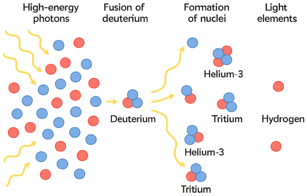
7.1. The Sakharov Conditions
Sakharov identified three general conditions required for a dynamical generation of baryon asymmetry from initially symmetric conditions [39]:
The first condition is necessary because a net baryon number cannot be generated if baryon number is exactly conserved. The second distinguishes matter from antimatter, while the third prevents detailed balance from cancelling the generated asymmetry.
These conditions are remarkably general and underlie most mechanisms proposed for baryogenesis, including grand-unified baryogenesis, electroweak baryogenesis and leptogenesis [40].
The Standard Model itself contains baryon-number violation through non-perturbative electroweak processes. At sufficiently high temperature, transitions between gauge vacua change baryon and lepton number according to
and therefore violate
while conserving
These processes, conventionally described through electroweak sphalerons, are efficient above the electroweak scale [41].
Thus the early Universe already contains a mechanism capable of changing baryon and lepton number. The remaining question is what produces the initial symmetry bias and, crucially, whether it generates a non-zero abundance that can survive sphaleron processing.
7.2. PT Breaking, CPT Symmetry and Charge Asymmetry
CPT invariance of the dynamical laws must also be distinguished from invariance of a selected cosmological state. A CPT-invariant theory can admit states that are not CPT invariant. The schematic group relation therefore does not imply that a PT-asymmetric branch of every CPT-invariant theory carries a nonzero charge or baryon number. If the state itself is assumed CPT invariant, the relation can constrain its discrete symmetries, but a matter yield still requires a specified charge-sensitive observable and transfer mechanism. In particular, temperature power modulation alone neither establishes a matter-sector CP bias nor supplies baryon- or lepton-number violation.
In a reheating model, a charge-sensitive source and baryon- or lepton-number-violating interactions must be calculated explicitly. A PT interpretation of a scalar temperature statistic is not by itself a demonstration of the required CP bias.
7.3. Reheating as the Transfer from Gravity to Matter
Quadratic gravity provides a particularly natural epoch at which such a transfer could occur. At the end of inflation, the scalaron oscillates around the minimum of its potential and decays into matter and radiation. The energy stored in the gravitational sector is thereby converted into the particle content of the hot Big Bang. The schematic evolution is
If the primordial gravitational state carries a PT asymmetry , reheating provides a natural stage at which this asymmetry could be transferred to the particle sector. The resulting matter–antimatter imbalance need not be generated instantaneously at the bounce itself. It may arise during scalaron decay or subsequently through interactions of the produced particles.
This observation is especially relevant because reheating is intrinsically a non-equilibrium process, thereby providing one of the Sakharov ingredients automatically.
The precise mechanism remains model dependent. Pure gravity coupled minimally to the Standard Model does not by itself guarantee the generation of baryon number. Additional baryon- or lepton-number-violating physics is still required. The point is instead that the finite-bounce scenario provides a natural symmetry bias and a natural non-equilibrium epoch in which this physics can operate. The proposed history provides a possible non-equilibrium epoch; a symmetry bias and its transfer must be derived in a particular state and particle model.
7.4. Leptogenesis and the Role of
One of the best-motivated possibilities is leptogenesis. In the original proposal of Fukugita and Yanagida, the out-of-equilibrium decays of heavy Majorana neutrinos generate a lepton asymmetry, which is subsequently converted partially into a baryon asymmetry by electroweak processes [42]. The essential quantity is not but
Electroweak sphalerons violate while preserving . Consequently, an asymmetry produced before the electroweak epoch survives most naturally if it contains a non-zero component.
For the Standard Model particle content, when the relevant interactions and sphalerons are in equilibrium, the final baryon yield is related to the primordial yield by [43]
This relation is central to the present discussion. It means that the problem can be separated into two stages:
followed by
through standard electroweak processing.
The finite-universe framework therefore does not need to generate the observed baryon abundance directly. It is sufficient for the quantum-to-classical transition to generate an appropriate asymmetry. Standard electroweak physics can then convert part of this into baryon number. This is precisely the logic underlying conventional leptogenesis [42,44], but here the origin of the initial asymmetry may be tied to the PT structure of the primordial gravitational state.
7.5. A Possible Scaling with and
We retain the possible reheating connection as a phenomenological target. With the standard equilibrium sphaleron conversion appropriate to the assumed particle content,
Here is an effective coefficient that includes production, transfer and washout; it is not necessarily a probability bounded by unity. Dimensional analysis does not determine the power of , since many dimensionless functions and additional mass ratios are possible. The proposed inverse- scaling is therefore an ansatz, not a derived consequence of quadratic gravity. Taking in a specified model convention and gives . This numerical illustration is not a prediction of the measured yield: for nonzero a freely adjustable can reproduce it. A quantitative test requires an independently calculated or constrained , baryon/lepton-number-violating interactions, the relevant CP structure and the thermal history. The microscopic mapping from to remains a separate prerequisite. For the illustrative choices above, the observed yield is reproduced by . This fits an effective coefficient; it does not independently predict the yield. The sphaleron factor assumes the Standard Model equilibrium conditions discussed in Eq. (109).
7.6. What Remains to Be Derived
Equation (112) is not yet a prediction of quadratic gravity or of PT-symmetric quantum theory. It is a phenomenological scaling motivated by the observed magnitudes of the relevant dimensionless quantities. A microscopic derivation must explain why the generated yield is proportional to , why the suppression scale is , and what determines the efficiency parameter .
This distinction becomes particularly important when comparing with conventional leptogenesis. If represented only the CP asymmetry per decay of a heavy particle, the final abundance would generally contain additional suppression factors associated with the number density of the decaying particles, washout and thermal efficiency. In that interpretation, one would not expect automatically to be of order unity.
For the direct scaling in Eq. (112) to hold, must instead characterize something closer to the comoving yield produced by the gravitational-to-matter transition, or the reheating dynamics must compensate the usual abundance and efficiency factors.
The result should therefore be viewed as a target for the microscopic theory rather than as an established derivation.
7.7. A Cosmological Consistency Test
An independent test becomes possible if a microscopic model fixes the primordial-state map, the inflationary normalization and the matter-production coefficient. Then a predicted can be compared with the nucleosynthesis/CMB determination. While is freely adjustable, agreement is only a fitted normalization. If a specified reheating and washout calculation cannot produce the measured yield, that matter-production mechanism is excluded, rather than the entire finite-bounce programme.
8. Relics of the Contracting Phase
A contracting phase permits nonlinear structures to form before the hot expanding era [14]. Whether they leave surviving perturbations depends on their dynamics through the high-density phase. This would be a second source of compact seeds, distinct from rare inflationary fluctuations. We retain the possibility and its statistical formulation below, without using a preliminary numerical abundance calculation as evidence for an allowed population.
8.1. Structure Formation During Contraction
For pressureless matter in the approximately flat, matter-dominated linear regime,
The solution grows as a decreases. Its density–velocity initial conditions differ from those of the usual growing mode in expansion; the mode mixture must therefore be specified. For a dominant mode with scale-independent growth , the smoothed variance is
Here q is a comoving wavenumber, distinct from the background curvature k, and R in the smoothing window is a comoving scale.
The Press–Schechter statistical construction is not restricted to an expanding background. For a Gaussian linearly evolved density field and a specified collapse barrier, the usual counting prescription has the same form,
The treatment of nested regions and the mass assignment retain their usual assumptions [45]. There is published precedent for applying this formalism to formation of black holes during contraction [46]; that application is not a calibration of virialized-halo abundances. Contraction is therefore not a reason to discard the statistical framework.
Likewise, the local pressureless spherical-collapse equation, in the matter-only approximation, does not change merely because the background contracts. What requires specification is its mapping to a linearly extrapolated contrast relative to that background. The familiar expanding Einstein–de Sitter value includes a particular growing-mode density–velocity relation and collapse criterion. It is not fixed by Gaussianity alone, and using the same numerical barrier for the contracting growing mode requires a corresponding spherical-collapse calculation. The formalism can thus be carried over, with contracting growth and the barrier appropriate to the chosen initial conditions. Using the empirical Sheth–Tormen calibration unchanged is a further assumption [47].
This discussion concerns classical, matter-dominated structure formation. Radiation, pressure, shear, tides or modified dynamics can alter the collapse calculation; the dust growth law is not extrapolated through the high-density bounce. These are qualifications on the physical input and calibration, not a failure of the Press–Schechter counting argument. Figure 7 illustrates the spherical-region construction.
Figure 7.
Configuration of a spherical collapse perturbation. We consider three spherically symmetric regions: (1) an outer background with radius and mean density ; (2) an inner region of radius with higher density ; and (3) an intermediate near-vacuum layer separating them. This can represent a collapsing overdensity of size R (a halo) within a larger universe of size r, or analogously, our finite Universe of radius R embedded in a larger space.
Figure 7.
Configuration of a spherical collapse perturbation. We consider three spherically symmetric regions: (1) an outer background with radius and mean density ; (2) an inner region of radius with higher density ; and (3) an intermediate near-vacuum layer separating them. This can represent a collapsing overdensity of size R (a halo) within a larger universe of size r, or analogously, our finite Universe of radius R embedded in a larger space.
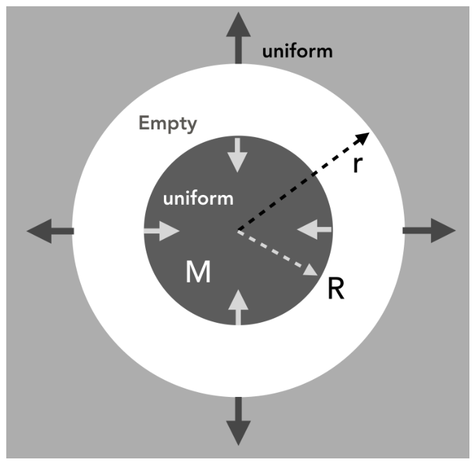
8.2. Virialization and Nonlinear Relic Seeds
Similarly, an expansion-era virial overdensity of order 200 and a radiation-era PBH threshold of order unity refer to different epochs, slicing conventions, profiles and physical problems. Their numerical comparison does not establish that a halo becomes a black hole after the bounce. Collapse at re-entry depends on compaction, profile, pressure, angular momentum and the local background. We use the pre-bounce population only as a candidate seed distribution with these uncertainties explicitly retained.
8.3. Apparent-Horizon Scale and the Survival Hypothesis
The geometrical scale used in the proposed survival prescription is
not . During density growth before the idealized high-density phase, can decrease; throughout the exact cosh bounce it is , and at the turning point it equals . The Hubble radius grows and diverges at the turning point; it cannot supply a shrinking survival scale through this solution.
A candidate criterion , with L a specified physical perturbation scale, must be followed over the entire interval of interest. For a comoving mode , the ratio decreases toward the turning point in the exact constant- solution; an earlier crossing need not persist to the bounce. Bound nonlinear objects need not follow and require a separate calculation. At , curvature-scale perturbations also cannot be modeled uncritically as small, isolated spherical halos in a locally flat background.
The proposal is that some contracting structures may retain identifiable perturbations through the high-density phase. Being outside an apparent horizon is not sufficient to freeze their internal dynamics or protect them from tidal evolution, mode mixing, dissipation or quantum-gravitational effects. We therefore leave survival as an explicit, presently uncalibrated transfer probability. A local black-hole horizon around a compact object, if present, must also be distinguished from the FLRW background apparent horizon.
The characteristic scales associated with the assumed density are
For an illustrative stellar-degeneracy-scale density, corresponds to ; corresponds to about . These rounded background scales are not a demonstrated relic-mass cutoff. Treating a stellar degeneracy density as a lower bound on is an additional physical assumption, not a universal bound for every completion.
8.4. Horizon Re-Entry and Relic Black Holes
The apparent horizon does not start growing immediately in the idealized constant-density phase. Re-entry must be followed through the later decreasing-density evolution, together with the size of the perturbation. Any black-hole formation on re-entry is conditional on the evolved profile and collapse dynamics.
Conditional on surviving nonlinear perturbations, the expanding matter field could contain an inflationary component and a relic component with different statistics. Neither the background apparent horizon nor the linear growth function fixes the conversion into black holes. That conversion enters the transfer description below.
8.5. From the Pre-Bounce Halo Population to the Relic Abundance
Let be a candidate comoving pre-bounce halo mass function at a specified epoch, using one scale-factor convention across the bounce. A more explicit replacement for an identity between halo and relic abundances is
where describes survival, mass transfer and conversion into a compact object. In a one-descendant approximation, its integral is at most unity; with fragmentation or mergers a more general population-evolution prescription is required. The identity-transfer ansatz is the special choice with complete survival. A step function at is only a toy prescription and does not derive this kernel.
The present physical density is then
with subsequent evaporation, accretion and mergers included in the evolution to today’s distribution. Choosing removes the explicit volume factor but not the need to specify it. Inflationary dilution and reheating are therefore material to any abundance estimate. A pre-bounce is a chosen normalization at a stated epoch and comoving length convention, not today’s measured .
The abundance depends on , the contracting spectrum, curvature, collapse calibration and the transfer prescription. We do not claim a robust numerical degeneracy slope or an excluded region without a reproducible calculation of these ingredients. The general relic mechanism remains an observational hypothesis [14].
8.6. Relics as Dark Matter
If relics are assigned to the cold-dark-matter budget, they must satisfy in the corresponding cosmological fit. This necessary budget condition is distinct from a baryon-density bound and is not a sufficient observational viability test. Lensing, dynamical, accretion and gravitational-wave constraints must be applied to the evolved mass function, with their astrophysical assumptions stated [4]. At present the condition constrains an assumed abundance model jointly with its survival and history parameters, not alone.
8.7. Seeds of Supermassive Black Holes
High-redshift massive black holes motivate studying additional seed channels [48,49]. Likewise, the abundance above a seed mass,
is only one input to a high-redshift black-hole model. Seed formation time, occupation, accretion duty cycle, mergers and observational selection must also be specified. A comparison with the local supermassive-black-hole density cannot alone establish a sufficient high-redshift seed population. We retain relics as a possible origin of massive seeds without claiming that a verified region of parameter space already reproduces the observed population. A comparison of a bounce density inferred this way with the scalaron plateau is conditional on both the abundance prescription and the proposed microscopic density relation.
8.8. Relics as Probes of the Bounce and the Contracting Phase
Different integrals of a single evolved relic mass function enter the dark-matter density, high-mass seed abundance, lensing, mergers and stochastic backgrounds. A joint analysis can constrain contracting initial conditions and bounce parameters only together with the collapse and transfer assumptions. The curvature normalization must also be related to present-day geometry through the full history in Equation (29). These observations could therefore probe a specified pre-bounce model, but do not currently provide a unique reconstruction of its initial spectrum or .
8.9. A Cross-Consistency Test of the Quantum-Gravity Scale
The hypothesized identification in natural units could connect inflationary normalization to relic physics. It is not yet a derivation of the bounce density. Comparing it with a relic constraint requires marginalizing over contracting growth, its barrier, the spectrum, survival, dilution and later evolution. A disagreement would reject the density identification within those assumptions; a robust agreement would be informative precisely because the relevant transfer had been independently specified.
Figure 8.
Quasi-normal ringing observed in the gravitational-wave signal from the first detected binary black-hole merger, GW150914. After the merger the newly formed black hole settles to equilibrium through damped oscillations known as quasi-normal modes. The frequency and decay time of the oscillation depend only on the mass and spin of the final black hole and provide a direct test of general relativity in the strong-field regime. Adapted from [50].
Figure 8.
Quasi-normal ringing observed in the gravitational-wave signal from the first detected binary black-hole merger, GW150914. After the merger the newly formed black hole settles to equilibrium through damped oscillations known as quasi-normal modes. The frequency and decay time of the oscillation depend only on the mass and spin of the final black hole and provide a direct test of general relativity in the strong-field regime. Adapted from [50].
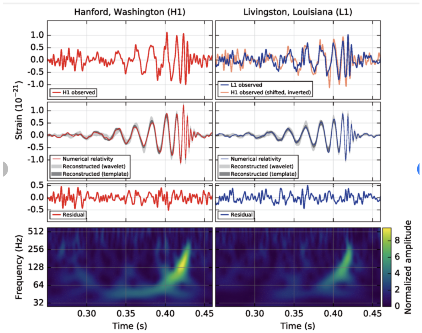
9. Strong-Gravity and Gravitational-Wave Tests
The cosmological observables discussed so far probe quantum gravity indirectly through the primordial Universe and the relic population inherited from the contracting phase. Black holes provide a complementary laboratory. Their near-horizon geometry accesses strong gravitational fields in the late Universe and can therefore test aspects of the same microscopic theory that controls the high-curvature dynamics of the bounce.
This complementarity is particularly important for quadratic gravity. In an exactly homogeneous FLRW background the Weyl tensor vanishes, so the background cosmological dynamics are controlled primarily by the sector. Around black holes, by contrast, the Weyl curvature is non-zero and the spin–2 sector becomes directly relevant [3,28]. Cosmology and black-hole observations therefore probe different components of the same gravitational action.
The basic observational strategy is to look for departures from the predictions of General Relativity in systems where the gravitational field is strongest. Particularly promising probes include black-hole ringdown, quasinormal-mode spectroscopy, horizon absorption, extreme-mass-ratio inspirals and possible parity-dependent signatures in gravitational waves [5,51,52].
9.1. Black-Hole Quasinormal Modes
After a perturbed black hole settles toward equilibrium, the emitted gravitational radiation is dominated by a discrete set of damped oscillations known as quasinormal modes [51]. Their complex frequencies can be written as
where determines the oscillation frequency and the decay rate.
In General Relativity, the quasinormal spectrum of an isolated Kerr black hole is determined entirely by its mass and angular momentum. Measuring several independent modes therefore provides a direct consistency test of the black-hole geometry and forms the basis of black-hole spectroscopy [52].
Higher-curvature modifications can alter both the background solution and the equations governing perturbations. In quadratic gravity, the Weyl-squared sector introduces additional spin–2 dynamics and can modify the quasinormal spectrum even when the large-scale geometry remains close to that of General Relativity [3,28].
The observational question is therefore whether the measured frequencies and damping times satisfy
for a single pair .
Any statistically significant inconsistency between multiple measured modes would indicate either additional degrees of freedom or a modification of the near-horizon gravitational dynamics.
9.2. Parity and Isospectrality
For a non-rotating Schwarzschild black hole, linear gravitational perturbations separate into axial and polar sectors. The axial sector is described by the Regge–Wheeler equation, while the polar sector is described by the Zerilli equation [53,54]. Although the two effective potentials are different, they possess the same quasinormal-mode spectrum,
This remarkable isospectrality reflects a hidden relation between the two perturbation equations and is discussed in detail in the classic treatment of black-hole perturbations by Chandrasekhar [55]. It therefore provides a particularly clean probe of the symmetry structure of the gravitational theory.
Modified gravity can break this relation. Extra scalar or tensor degrees of freedom can couple differently to the two parity sectors, producing
Schwarzschild isospectrality is a relation between its perturbation equations, not a direct consequence of fundamental PT invariance. It can be broken in parity-preserving modified theories. A test of axial and polar responses therefore probes the specified perturbation dynamics rather than establishing PT violation by itself.
9.3. Additional Gravitational Degrees of Freedom
The scalaron normalization in the inflationary example gives . By comparison,
Here is expressed as a rest energy in natural units. Ordinary astrophysical ringdown therefore cannot directly excite this heavy scalaron on shell. In a simple decoupling expansion a correction proportional to would be of order at this frequency; this is only an illustration of the scale hierarchy, not a derived ringdown shift.
The Weyl sector has a separately controlled scale, schematically , and is not constrained to the scalaron mass by . Nonzero Weyl curvature alone does not imply an observable correction. In conventional quadratic gravity, Schwarzschild remains a solution and its axial spectrum includes the GR modes together with additional massive spin-2 modes; other background branches can have different spectra [56]. Detectability depends on the allowed mass scale, stable background branch, coupling, excitation amplitude, propagation and detector response.
The quantization prescription is essential. The proposal discussed in Ref. [29] treats the extra spin-2 sector as absent from the physical asymptotic particle spectrum. One cannot import observable propagating massive-mode predictions from a different prescription without deriving the retarded response and boundary conditions in that theory. The homogeneous FLRW result does not remove Weyl-sector effects from perturbations, but neither does it fix their size.
We therefore present spectroscopy, absorption and EMRI phasing as research directions rather than demonstrated sensitivity to this specific completion. A forecast requires an effect size in an independently viable parameter range and a comparison with instrumental, waveform and astrophysical uncertainties. Axial–polar isospectrality can fail in parity-preserving modified theories and is not by itself a test of fundamental PT violation. Reflective horizon models likewise need an independently specified response; reflection does not follow merely from an or term. A significant deviation from a GR waveform also requires conventional modeling and environmental explanations to be assessed before assigning it to quantum gravity. LISA provides a concrete future setting for EMRI studies [57], without guaranteeing sensitivity to every microscopic completion.
9.4. Horizon Absorption
Another clean strong-gravity observable is the absorption of gravitational radiation by a black-hole horizon.
In General Relativity, part of the gravitational-wave flux produced by an orbiting object is absorbed by the horizon [58]. Using positive outward and absorbed energy fluxes, the orbital balance is
where describes net energy extraction in a superradiant regime.
The magnitude and sign of depend on the black-hole spin and the frequency of the perturbation. For rapidly rotating black holes, superradiant interactions can even make the effective horizon flux negative [59].
Any modification of the microscopic horizon structure may alter this absorption. A perfectly reflecting or partially reflecting quantum boundary, for example, would give a different flux from a classical absorbing horizon [5].
Measurements of horizon absorption therefore provide a direct probe of whether astrophysical black holes possess the dissipative properties predicted by General Relativity.
9.5. Extreme-Mass-Ratio Inspirals
Extreme-mass-ratio inspirals provide one of the most precise future probes of black-hole geometry [60,61]. In these systems, a stellar-mass compact object orbits a massive black hole for thousands to millions of cycles before merger.
The accumulated gravitational-wave phase is extremely sensitive to the background geometry and to small corrections in the radiation-reaction force. Schematically,
so that even a very small fractional modification of the orbital evolution can accumulate into an observable phase shift over the full inspiral.
EMRIs can therefore test several aspects of strong gravity simultaneously: the multipole structure of the central object, horizon absorption, additional gravitational degrees of freedom and possible deviations from the Kerr metric.
This makes them particularly complementary to ringdown observations. Ringdown probes the response of the black hole after a violent perturbation, whereas an EMRI maps the geometry and dissipative properties of the same object over a long period of quasi-adiabatic evolution.
These systems are among the principal science targets of LISA [60], which should provide access to long-duration inspirals into massive black holes and thereby substantially improve tests of near-horizon gravity.
9.6. Primordial and Astrophysical Gravitational Waves
Gravitational waves also connect the strong-gravity and cosmological components of the framework.
A high-curvature bounce and the subsequent inflationary phase can produce a primordial tensor background,
whose amplitude, scale dependence and parity structure depend on the microscopic gravitational theory.
If the primordial state breaks PT symmetry, the two tensor helicities may have different spectra,
Such chirality can be tested through CMB polarization and, depending on the frequency range and transfer function, potentially through direct gravitational-wave observations.
At later times, the relic population discussed in the previous section can generate an independent astrophysical gravitational-wave background through binary formation and mergers.
The total signal may therefore contain two conceptually different components,
The first probes the quantum state and high-curvature dynamics directly, while the second probes the surviving population of structures formed during contraction.
9.7. A Hierarchy of Strong-Gravity Tests
The strongest conclusions will not come from any single departure from General Relativity but from consistency among several independent observables.
For black holes, the relevant chain is
Each observable probes a different aspect of the same near-horizon physics. For example, a modification that shifts the quasinormal spectrum but leaves horizon absorption exactly unchanged would have to be consistent with the same underlying perturbation equations. Likewise, an additional spin–2 degree of freedom inferred from ringdown should also affect propagation or orbital dynamics in a predictable way.
This creates a network of internal consistency tests that is much harder to satisfy accidentally than a single anomalous measurement.
9.8. Connecting Black Holes and the Cosmological Bounce
Cosmology and astrophysical black holes probe different regimes of a candidate gravitational theory. Homogeneous scalaron inflation constrains the sector under its state and reheating assumptions, while a calculated black-hole response can probe the Weyl sector if its mass scale and couplings are accessible. These couplings are independent unless the microscopic theory relates them. A nonzero Weyl tensor is not sufficient to establish an observable correction, and the physical spectrum must be derived in the chosen quantization. The complementarity is therefore a programme for a specified completion rather than a demonstrated observational determination of both couplings.
10. Cross-Consistency Tests
The purpose of cross-consistency tests is to compare predictions of a specified common theory across different observations. Multiple channels do not by themselves establish an over-constraint. In addition to , , and the contracting spectrum and curvature, the current construction contains state, reheating, matter-production and relic-transfer inputs. Table 1 distinguishes their status.
10.1. The Inflationary Normalization:
Under conventional scalaron slow roll and the usual state, , as discussed in Section 6.2. The measured scalar amplitude constrains the coupling only after the pivot-to- mapping, reheating and state are specified. It then fixes the scalaron mass and plateau scale within that model, without by itself fixing the bounce density or the independent Weyl coupling.
10.2. A First Consistency Loop: , and
The proposed relation is a hypothesis about the effective state, not a consequence of the finite region or of the inflationary normalization alone. A test compares the density predicted by a microscopic completion with that required by a specified relic model, including its spectrum and transfer uncertainties. Failure would reject this connection; it would not in itself invalidate scalaron inflation or every bounce.
10.3. A Second Consistency Loop: , and
For a defined primordial-state map and inflationary history, the ansatz gives
This relates quantities obtained from different phenomena, but it is not an independent prediction while is free. Temperature data also do not determine without a state/transfer model. A microscopic production and washout calculation, together with the state map, is needed before the baryon abundance tests this connection.
10.4. A Third Consistency Loop: Curvature and the Initial Collapse
Spatial curvature could constrain a model of the initial contracting region when its scale-factor normalization, duration of contraction, inflation and thermal history are specified. Constant k alone is not an observable memory. Equation (29) determines how at two nonsingular-Hubble epochs is related. A comparison with curvature inferred in a relic analysis is therefore conditional on both histories and the population model; sufficient inflation can suppress the present signal.
10.5. The Relic Consistency Triangle
The total relic density, abundance above a seed mass, lensing and merger statistics can test different parts of one evolved mass function. The cold-dark-matter budget is only a necessary condition. A common fit must include the collapse barrier, transfer kernel, dilution, mass evolution and the selection functions of the observations. These are potentially complementary constraints, not yet independent measurements of a microscopically predicted population.
10.6. The PT Consistency Triangle
The same distinction applies to the PT comparison. Rather than requiring raw amplitudes inferred from , polarization and tensors to be equal, a specified model must predict the separate transfer functions and which signals vanish. Correlations between CMB estimators and between cosmological parameter determinations must be retained. Independent physical channels are valuable, but they are not automatically statistically independent measurements of one known parameter.
10.7. The Strong-Gravity Consistency Triangle
Ringdown, horizon absorption and EMRI phasing must follow from a common response model if used to test one completion. A viable parameter range, excitation amplitudes and observational sensitivity are required. A null measurement excludes only a predicted detectable effect, and a departure from axial–polar isospectrality is not by itself fundamental parity violation. The mass and quantization of the extra sector remain essential inputs.
10.8. Connecting the Ricci and Weyl Sectors
The homogeneous FLRW background has , while black-hole geometries can have nonzero Weyl curvature. This distinction motivates complementary tests but does not impose a relation between and . A theory linking them must derive it and propagate it to observables in the appropriate background and quantization. A common action alone is not a forecast of detectable cross-sector effects.
10.9. An Observational Network
The present parameter list must include not only and the contracting spectrum and curvature, but also the primordial-state prescription, reheating history, , collapse parameters, relic transfer and astrophysical evolution. Multiple channels become an over-constraint only when enough observable relations are predicted with shared parameters and the remaining freedom and data covariances are accounted for. With freely adjustable, the proposed baryon yield fits a normalization rather than predicting it. With an unconstrained , relic observations do not uniquely measure .
The complete framework can be summarized as a network shown in Figure 9 rather than a linear chain. The arrows in this diagram do not all represent established theoretical relations. Some are predictions of well-developed components of the framework, others are hypotheses that require microscopic derivation. That distinction is precisely what makes the network useful: each proposed connection can be tested independently.
10.10. From Parameter Fitting to Over-Constraining the Theory
The goal is to construct a restricted implementation whose joint likelihood depends on a specified common parameter set, with priors and theoretically justified nuisance parameters. A demonstration of over-constraint would require the observable–parameter relations, their independent information content and their degeneracies; it has not been provided here. Deriving a bounce density from , a matter-production coefficient from reheating and a relic transfer prescription would move the programme toward this goal.
10.11. What Would Falsify the Framework?
The scope of any exclusion should be stated precisely. Incompatible inflationary and relic density scales would reject the proposed density identification within the adopted relic model. Failure of a predicted polarization or tensor signal would reject the state/transfer model that actually predicts it; a null measurement does not reject a scalar even–odd modulation with . An incorrect baryon yield would exclude a specified microphysical production mechanism. Excess lensing, mergers or seed abundance would exclude the specified evolved mass function. Curvature comparisons would test a specified contraction, inflation and thermal history. Strong-gravity data would exclude a completion only where it predicts a detectable response that the observations rule out.
None of these failures automatically excludes every finite or bouncing cosmology. The broader idea allows different microscopic dynamics and initial conditions; it becomes falsifiable only through sufficiently specified realizations. This distinction keeps the programme testable without claiming that every null observation rejects global finiteness or a pre-bounce history.
10.12. The Universe as a Laboratory
A specified finite-bounce history could connect observables separated by many orders of magnitude in time and scale. Its value would come from the consistency of independently calculated predictions, with covariance and remaining parameter freedom included. This is a possible observational laboratory, not a claim that present anomalies already establish a unique microscopic history.
11. Discussion and Outlook
The purpose of this review has been to explore a different way of approaching quantum gravity. Rather than beginning with a microscopic theory and asking how effects confined to extremely short distances might eventually become observable, we have started from a global hypothesis: that the FLRW cosmology we observe may admit a finite global completion. We then asked what observable consequences can follow if such a finite gravitating region undergoes collapse, reaches a high-density quantum state and subsequently re-expands.
This distinction between local cosmology and global completion is important. Present observations do not establish that the Universe is globally finite. They do, however, establish within CDM a positive cosmological constant and hence a finite asymptotic causal horizon. The conventional construction continues the same homogeneous FLRW solution indefinitely beyond that horizon. The finite framework considered here explores a different possibility: the local FLRW dynamics can remain unchanged while the cosmological region belongs to a finite gravitating spacetime. In the Schwarzschild realization reviewed here, the asymptotic de Sitter and gravitational horizon scales coincide,
This relation is a property of that particular global completion and not a consequence of finiteness alone.
The Black Hole Universe provides a concrete realization of this perspective. A finite overdensity can originate through gravitational instability within a larger background, become gravitationally bound and undergo collapse. Within the class of models considered here, positive spatial curvature and a finite limiting density then provide the two ingredients required for a regular homogeneous bounce. The expanding Universe need not represent an absolute beginning, but can instead be the post-bounce branch of a longer gravitational history.
The existence of a regular homogeneous solution is not, however, sufficient to establish the viability of this history. Anisotropies and perturbations can grow during contraction, and the stability of the bounce must ultimately be demonstrated within the microscopic completion. This is not merely a technical qualification but an additional falsifiability criterion. A viable theory must either keep these perturbations under control throughout the finite contraction or provide high-density dynamics that modify their classical growth before they backreact strongly on the background.
This separation between the global cosmological framework and the microscopic quantum theory is one of the useful features of the construction. The finite-bounce picture does not require one unique theory of quantum gravity. Its role is to provide a setting in which candidate theories can be confronted with observations. A successful microscopic completion should determine, or at least constrain, the limiting density and duration of the high-density state, its stability, the primordial fluctuation spectrum, the symmetry structure of the quantum state and the transition from gravitational degrees of freedom to matter and radiation.
Quadratic gravity provides one particularly useful worked example. Its sector generates the quasi-de Sitter dynamics underlying scalaron inflation, and within a specified inflationary state and reheating history the observed scalar amplitude constrains the coupling . This fixes a characteristic high-curvature scale. Whether that scale also determines the bounce density,
remains a hypothesis rather than a derived result. Precisely for that reason it is useful: if a microscopic completion predicts this relation, the bounce scale inferred from relic or other pre-bounce phenomena becomes an independent consistency test of the same theory. The Weyl sector similarly provides a possible connection to strong-gravity observations, but only when its mass scale, quantization and physical response make the additional degrees of freedom observationally accessible.
PT completion provides a complementary example concerning the quantum state rather than its characteristic energy scale. A complete PT-symmetric state can contain semiclassical sectors with opposite time orientations while an observer inhabits only one of them. This opens a possible route to connecting two long-standing problems. The low gravitational entropy conventionally encoded in the Past Hypothesis need not necessarily be imposed as an absolute initial boundary condition, while information associated with the contracting branch need not be destroyed simply because it is inaccessible in the classical expanding branch. In a unitary PT-complete description, apparent information loss may instead reflect restricted semiclassical accessibility. The analogy with ER=EPR is suggestive: causal or geometrical separation need not imply factorization of the underlying quantum state. This does not yet constitute a microscopic derivation of the Past Hypothesis or the arrow of time, but it turns both into questions that can, in principle, be addressed within the same quantum transition.
The observational significance of PT completion lies in the possibility that branch selection leaves measurable symmetry information in primordial perturbations. Large-angle CMB temperature statistics provide a concrete model-comparison test of the direct-sum realization, but an even–odd power imbalance alone does not establish fundamental parity or PT violation. The mapping to an effective is model dependent and must be tested independently through polarization, tensor modes and other parity-sensitive observables. Likewise, a connection between , reheating and the baryon asymmetry remains phenomenological until a charge-sensitive production mechanism and its washout dynamics are derived.
The contracting phase introduces another potentially observable record. Gravitational instability can generate nonlinear structures before the bounce, providing candidate seeds that are distinct from the nearly Gaussian fluctuations generated during inflation. Their survival is not guaranteed by crossing the FLRW apparent horizon, and the transfer through the high-density phase remains an open dynamical problem. The appropriate description therefore contains a survival and mass-transfer kernel rather than an assumed one-to-one mapping between pre-bounce halos and present relics. If this transfer can be calculated, dark-matter abundance, massive high-redshift seeds, lensing, merger rates and stochastic gravitational-wave backgrounds become different measurements of the same evolved relic population.
Strong-gravity observations provide a further, complementary laboratory. Black-hole ringdown, horizon absorption and extreme-mass-ratio inspirals can test additional gravitational degrees of freedom and near-horizon response, but strong curvature alone does not guarantee sensitivity to a given ultraviolet completion. In particular, the scalaron mass inferred from inflation is enormously above astrophysical frequencies, while the Weyl-sector scale is independent unless the microscopic theory relates the two. These observations should therefore be viewed as tests of specified completions with calculable responses rather than generic signatures of finite cosmology.
The principal outcome of the review is consequently not a claim that all of these links have already been derived. It is an organization of the problem into a network of relations with different levels of theoretical maturity. Some are established within specified models, such as the relation between and in scalaron inflation. Others are model-specific primordial calculations, conditional population models or phenomenological targets that still require a microscopic derivation. The status table and dependency network introduced above are intended to make these distinctions explicit.
This also clarifies what it would mean to falsify the programme. Failure of a particular relation between and would reject that identification, not every bouncing cosmology. Failure of a predicted polarization or tensor signal would test the corresponding primordial-state model. An incorrect baryon yield would exclude a specified matter-production mechanism. Relic observations can reject a given evolved mass function once its transfer history is fixed, while strong-gravity observations can constrain a microscopic completion only in regimes where it predicts a detectable response. Stability of the contracting branch itself provides another direct test: a completion that cannot prevent destructive anisotropic or perturbative backreaction would fail before any late-time observational comparison is required.
The goal is therefore not to accumulate unrelated anomalies, but to reduce the remaining freedom until multiple observations test a common microscopic parameter set. Only at that stage does the framework become genuinely over-constrained. The present construction should be regarded as a programme for reaching that point rather than as a demonstration that it has already been achieved.
The broader motivation nevertheless remains unchanged. If the observed expansion emerged from the high-density endpoint of a previous gravitational collapse, then quantum gravity has already acted on the entire observable Universe. Its effects need not remain confined to an inaccessible microscopic regime. The Universe itself has explored energies, curvatures, horizons and timescales that cannot be reproduced experimentally on Earth. CMB and galaxy maps, black holes and gravitational waves can therefore be interpreted as experiments performed by Nature, each probing a different aspect of the same underlying gravitational physics. In this sense the programme developed here is complementary to theory-first approaches such as string theory, loop quantum gravity, higher-curvature gravity or other microscopic modifications: instead of asking only which quantum theory is mathematically consistent, one asks which candidate theory can account simultaneously for the records that Nature has already provided.
The Universe can therefore preserve information about its quantum-gravitational history across an extraordinary hierarchy of scales. The central challenge is to determine whether those apparently different records converge on a common microscopic description or instead falsify the proposed connections. If they converge, quantum gravity may become accessible not through a single decisive experiment, but through the consistency of cosmology, particle physics and strong-gravity observations.
A finite Universe would then be more than a possible global completion of the observed cosmology. It would provide a natural laboratory for quantum gravity.
Funding
This work was partially supported by grants from Spain Plan Nacional (PGC2018-102021-B-100) and Maria de Maeztu (CEX2020-001058-M) and from European Union LACEGAL 734374 and EWC 776247. IEEC is funded by Generalitat de Catalunya.
Data Availability Statement
No new data are presented.
Acknowledgments
I would like to express my deepest gratitude to Emilio Elizalde, who supervised my PhD and has played a uniquely important role in my scientific life. He was my co-author on my first research paper, supported me at crucial stages of my career and, with great generosity, encouraged me as I developed an independent scientific path of my own. Over the years our relationship grew from that of supervisor and student into a long-standing collaboration and friendship, and we shared much of the scientific life of the institute that he helped to create. Emilio’s generosity has never been limited to science itself: he has consistently supported the careers and independence of his students and colleagues. It is therefore especially meaningful for me to contribute this review to a volume celebrating his 75th birthday, with deep gratitude for his guidance, friendship and support over more than three decades.
Conflicts of Interest
The author declares no conflict of interest.
References
- Battefeld, D.; Peter, P. A Critical Review of Classical Bouncing Cosmologies. Physics Reports 2015, 571, 1–66, [arXiv:astro-ph.CO/1406.2790]. [CrossRef]
- Brandenberger, R.; Peter, P. Bouncing Cosmologies: Progress and Problems. Foundations of Physics 2017, 47, 797–850, [arXiv:hep-th/1603.05834]. [CrossRef]
- Salvio, A. Quadratic Gravity. Frontiers in Physics 2018, 6, 77, [1804.09944]. [CrossRef]
- Green, A.M. Primordial Black Holes as a Dark Matter Candidate—A Brief Overview. Nuclear Physics B 2024, 1003, 116494, [arXiv:astro-ph.CO/2402.15211]. [CrossRef]
- Cardoso, V.; Pani, P. Testing the Nature of Dark Compact Objects: A Status Report. Living Reviews in Relativity 2019, 22, 4, [1904.05363]. [CrossRef]
- Gaztañaga, E. Boundary Terms, Finite FLRW Spacetimes, and the Emergence of the Cosmological Constant. Preprints.org 2026. [CrossRef]
- Oppenheimer, J.R.; Snyder, H. On Continued Gravitational Contraction. Physical Review 1939, 56, 455–459.
- Misner, C.W.; Sharp, D.H. Relativistic Equations for Adiabatic, Spherically Symmetric Gravitational Collapse. Phys. Rev. 1964, 136, B571–B576. [CrossRef]
- Peebles, P.J.E. The large-scale structure of the universe; 1980.
- Weinberg, S. The cosmological constant problem. Reviews of Modern Physics 1989, 61, 1–23. [CrossRef]
- Carroll, S.M.; Press, W.H.; Turner, E.L. The cosmological constant. ARAA 1992, 30, 499–542. [CrossRef]
- Elizalde, E.; Gaztañaga, E. On the probability distribution for the cosmological constant. Physics Letters B 1990, 234, 265–270. [CrossRef]
- Gaztañaga, E.; Kumar, K.S.; Pradhan, S.; Gabler, M. Gravitational bounce from the quantum exclusion principle. PRD 2025, 111, 103537, [2505.23877]. [CrossRef]
- Gaztañaga, E. Cosmological bounce relics: Black holes, gravitational waves, and dark matter. Phys. Rev. D 2026, 113, 043544, [2602.17702]. [CrossRef]
- Feynman, R.P.; Hibbs, A.R. Quantum Mechanics and Path Integrals; McGraw-Hill: New York, 1965.
- Gell-Mann, M.; Hartle, J.B. Quantum Mechanics in the Light of Quantum Cosmology. Complexity, Entropy, and the Physics of Information 1990, 8, 425–458.
- Halliwell, J.J. Introductory Lectures on Quantum Cosmology. Quantum Cosmology and Baby Universes 1991, pp. 159–243, [arXiv:gr-qc/0909.2566].
- Dodelson, S. Modern cosmology, Academic Press, NY; 2003.
- Cai, Y.F.; Brandenberger, R.; Peter, P. Anisotropy in a Nonsingular Bounce. Classical and Quantum Gravity 2013, 30, 075019, [1301.4703]. [CrossRef]
- Grain, J.; Vennin, V. Unavoidable Shear from Quantum Fluctuations in Contracting Cosmologies. European Physical Journal C 2021, 81, 132, [2005.04222]. [CrossRef]
- Battefeld, T.J.; Brandenberger, R.H. Vector Perturbations in a Contracting Universe. Physical Review D 2004, 70, 121302, [hep-th/0406180]. [CrossRef]
- Zhu, M.; Chen, C. Constraining Matter-Bounce Scenario from Scalar-Induced Vector Perturbations. Physical Review D 2025, 112, 023549, [2409.09458]. [CrossRef]
- Libanov, M.; Mironov, S.; Rubakov, V. Generalized Galileons: Instabilities of Bouncing and Genesis Cosmologies and Modified Genesis. Journal of Cosmology and Astroparticle Physics 2016, 08, 037, [1605.05992]. [CrossRef]
- Kobayashi, T. Generic Instabilities of Nonsingular Cosmologies in Horndeski Theory: A No-Go Theorem. Physical Review D 2016, 94, 043511, [1606.05831]. [CrossRef]
- Lin, C.; Quintin, J.; Brandenberger, R.H. Massive Gravity and the Suppression of Anisotropies and Gravitational Waves in a Matter-Dominated Contracting Universe. Journal of Cosmology and Astroparticle Physics 2018, 01, 011, [1711.10472]. [CrossRef]
- Mironov, S.; Rubakov, V.; Volkova, V. Genesis with General Relativity Asymptotics in Beyond Horndeski Theory. Physical Review D 2019, 100, 083521, [1905.06249]. [CrossRef]
- Ilyas, A.; Zhu, M.; Zheng, Y.; Cai, Y.F.; Saridakis, E.N. DHOST Bounce. Journal of Cosmology and Astroparticle Physics 2020, 09, 002, [2002.08269]. [CrossRef]
- Stelle, K.S. Renormalization of Higher-Derivative Quantum Gravity. Phys. Rev. D 1977, 16, 953.
- Sravan Kumar, K.; Marto, J. Unitary Quadratic Quantum Gravity in 4D. arXiv e-prints 2026, p. arXiv:2604.19707, [arXiv:hep-th/2604.19707]. [CrossRef]
- Gaztañaga, E.; Sravan Kumar, K.; Marto, J. A new understanding of Einstein–Rosen bridges. Classical and Quantum Gravity 2026, 43, 015023. [CrossRef]
- Einstein, A.; Rosen, N. The Particle Problem in the General Theory of Relativity. Phys. Rev. 1935, 48, 73–77. [CrossRef]
- Schrödinger, E. Expanding Universe; Cambridge University Press, 1956.
- ’t Hooft, G. Black Hole Unitarity and Antipodal Entanglement. Foundations of Physics 2016, 46, 1185–1198. [CrossRef]
- Maldacena, J.; Susskind, L. Cool horizons for entangled black holes. Fortschr. Phys. 2013, 61, 781.
- Akrami, Y.; et al. Planck 2018 results. VII. Isotropy and Statistics of the CMB. Astron. Astrophys. 2020, 641, A7, [1906.02552]. [CrossRef]
- Gaztañaga, E.; Kumar, K.S. Finding origins of CMB anomalies in the inflationary quantum fluctuations. JCAP 2024, 06, 001, [2401.08288]. [CrossRef]
- Planck Collaboration.; Ade, P.A.R.; Aghanim, N.; Armitage-Caplan, C.; Arnaud, M.; Ashdown, M.; Atrio-Barand ela, F.; Aumont, J.; Baccigalupi, C.; Banday, A.J.; et al. Planck 2013 results. XXIII. Isotropy and statistics of the CMB. A & A 2014, 571, A23, [1303.5083]. [CrossRef]
- Collaboration, P. Planck 2018 results. VI. Cosmological parameters. arXiv e-prints 2018, p. arXiv:1807.06209, [1807.06209].
- Sakharov, A.D. Violation of CP Invariance, C Asymmetry, and Baryon Asymmetry of the Universe. JETP Letters 1967, 5, 24–27.
- Riotto, A.; Trodden, M. Recent Progress in Baryogenesis. Annual Review of Nuclear and Particle Science 1999, 49, 35–75, [hep-ph/9901362]. [CrossRef]
- Kuzmin, V.A.; Rubakov, V.A.; Shaposhnikov, M.E. On Anomalous Electroweak Baryon-Number Non-Conservation in the Early Universe. Physics Letters B 1985, 155, 36–42. [CrossRef]
- Fukugita, M.; Yanagida, T. Baryogenesis Without Grand Unification. Physics Letters B 1986, 174, 45–47. [CrossRef]
- Harvey, J.A.; Turner, M.S. Cosmological Baryon and Lepton Number in the Presence of Electroweak Fermion-Number Violation. Physical Review D 1990, 42, 3344–3349. [CrossRef]
- Buchmüller, W.; Peccei, R.D.; Yanagida, T. Leptogenesis as the Origin of Matter. Annual Review of Nuclear and Particle Science 2005, 55, 311–355, [hep-ph/0502169]. [CrossRef]
- Press, W.H.; Schechter, P. Formation of Galaxies and Clusters of Galaxies by Self-Similar Gravitational Condensation. ApJ 1974, 187, 425–438. [CrossRef]
- Quintin, J.; Brandenberger, R.H. Black Hole Formation in a Contracting Universe. Journal of Cosmology and Astroparticle Physics 2016, 2016, 029, [arXiv:astro-ph.CO/1609.02556]. [CrossRef]
- Sheth, R.K.; Tormen, G. Large-scale bias and the peak background split. MNRAS 1999, 308, 119–126.
- Bañados, E.; Venemans, B.P.; Mazzucchelli, C.; et al. An 800-million-solar-mass black hole in a significantly neutral Universe at a redshift of 7.5. Nature 2018, 553, 473–476. [CrossRef]
- Zhu, Q.; et al. The growth of the gargantuan black holes powering high-redshift quasars and their impact on the formation of early galaxies and protoclusters. Monthly Notices of the Royal Astronomical Society 2024, 527, 1033–1054. [CrossRef]
- Abbott, B.P.e.a. Observation of Gravitational Waves from a Binary Black Hole Merger. Physical Review Letters 2016, 116, 061102. [CrossRef]
- Berti, E.; Cardoso, V.; Starinets, A.O. Quasinormal modes of black holes and black branes. Classical and Quantum Gravity 2009, 26, 163001. [CrossRef]
- Berti, E.; et al. Testing General Relativity with Present and Future Astrophysical Observations. Classical and Quantum Gravity 2015, 32, 243001, [1501.07274]. [CrossRef]
- Regge, T.; Wheeler, J.A. Stability of a Schwarzschild singularity. Physical Review 1957, 108, 1063–1069. [CrossRef]
- Zerilli, F.J. Effective potential for even-parity Regge–Wheeler gravitational perturbation equations. Physical Review Letters 1970, 24, 737–738. [CrossRef]
- Chandrasekhar, S. The Mathematical Theory of Black Holes; Oxford University Press, 1983.
- Antoniou, G.; Gualtieri, L.; Pani, P. Gravitational Quasinormal Modes of Black Holes in Quadratic Gravity. Physical Review D 2025, 111, 064059, [arXiv:gr-qc/2412.15037]. [CrossRef]
- Colpi, M.; Danzmann, K.; Hewitson, M.; et al. LISA Definition Study Report 2024. [arXiv:astro-ph.CO/2402.07571]. [CrossRef]
- Poisson, E. Absorption of Mass and Angular Momentum by Black Holes: The Time-Domain Formalism. Physical Review D 2004, 70, 084044, [gr-qc/0407050]. [CrossRef]
- Brito, R.; Cardoso, V.; Pani, P. Superradiance. Lecture Notes in Physics 2015, 906, 1–237, [1501.06570]. [CrossRef]
- Amaro-Seoane, P.; et al. Intermediate and Extreme Mass-Ratio Inspirals—Astrophysics, Science Applications and Detection Using LISA. Classical and Quantum Gravity 2007, 24, R113–R169, [astro-ph/0703495]. [CrossRef]
- Barack, L.; Pound, A. Self-Force and Radiation Reaction in General Relativity. Reports on Progress in Physics 2019, 82, 016904, [1805.10385]. [CrossRef]
Figure 4.
The top panels show the anti-symmetric, , component of the Planck 2018 CMB normalized temperature map ([35]) in North and South polar galactic caps. The visualization is such that the Galactic plane remains obscured along the edges. Parity conjugate positions can be identified by horizontally flipping into the opposite pole, where both caps have the same information with opposing signs: . The bottom panel presents the observed maps, including both the symmetric and anti-symmetric components. The evident resemblance between the top and bottom panels indicates the prevalence of the anti-symmetric component.
Figure 4.
The top panels show the anti-symmetric, , component of the Planck 2018 CMB normalized temperature map ([35]) in North and South polar galactic caps. The visualization is such that the Galactic plane remains obscured along the edges. Parity conjugate positions can be identified by horizontally flipping into the opposite pole, where both caps have the same information with opposing signs: . The bottom panel presents the observed maps, including both the symmetric and anti-symmetric components. The evident resemblance between the top and bottom panels indicates the prevalence of the anti-symmetric component.
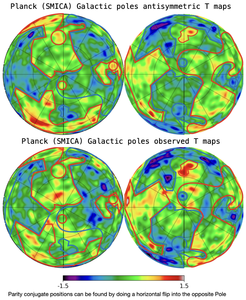
Figure 9.
Network of cross-consistency tests in a finite bouncing cosmology. Rounded filled boxes denote observables, while square boxes denote theoretical parameters or intermediate model predictions. The CMB scalar amplitude fixes the coupling , while the CMB parity signal determines . These quantities enter the reheating and baryogenesis sector. The bounce density and the pre-bounce perturbation spectrum determine the relic mass function, whose different moments are constrained by the total relic density and the abundance of massive black-hole seeds. Strong-gravity observables independently probe the Weyl/spin–2 sector. Dashed arrows denote proposed microscopic or cross-consistency relations that remain to be derived.
Figure 9.
Network of cross-consistency tests in a finite bouncing cosmology. Rounded filled boxes denote observables, while square boxes denote theoretical parameters or intermediate model predictions. The CMB scalar amplitude fixes the coupling , while the CMB parity signal determines . These quantities enter the reheating and baryogenesis sector. The bounce density and the pre-bounce perturbation spectrum determine the relic mass function, whose different moments are constrained by the total relic density and the abundance of massive black-hole seeds. Strong-gravity observables independently probe the Weyl/spin–2 sector. Dashed arrows denote proposed microscopic or cross-consistency relations that remain to be derived.
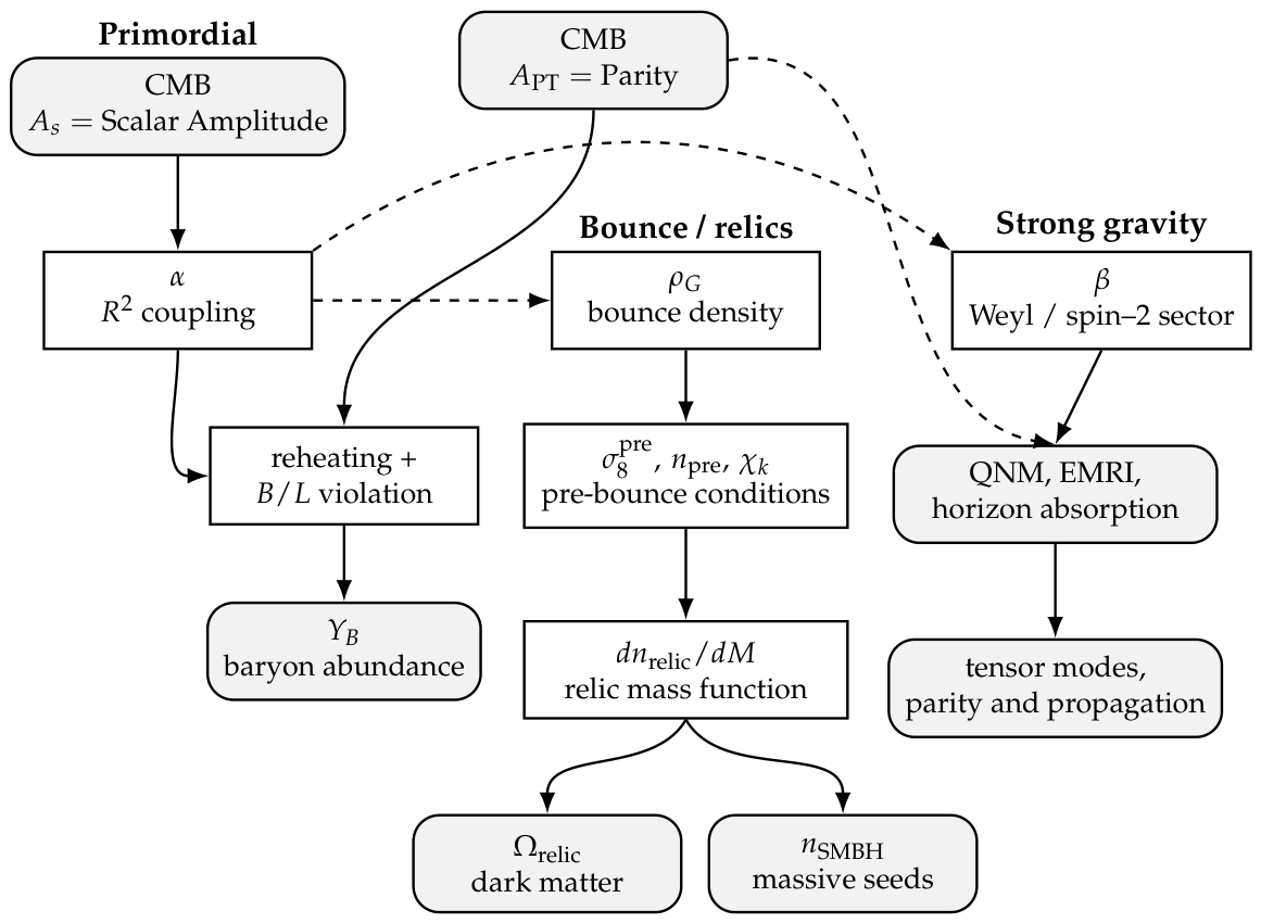

Table 1.
Status of the relations used in the observational programme.
| Status | Relation or result | Scope and unresolved input |
|---|---|---|
| Established geometrical result | FLRW ; null-expansion signs | A local horizon classification, not a survival theorem or global event-horizon construction. |
| Model-specific background | Constant-density, cosh bounce | Regular homogeneous effective solution; microscopic state and stability not derived here. |
| Established within a specified inflationary model | Conventional scalaron slow roll and state; reheating fixes the pivot mapping. | |
| Model-specific primordial calculation | DSI temperature modulation | Tests a specified spectrum; even–odd imbalance alone is not statistical parity violation. |
| Global Completion | Schwarzschild exterior and compatible stationary null asymptotics | |
| Phenomenological identification | Requires a common microscopic description and consistent units/frame. | |
| Phenomenological yield | Transfer, charge-violating dynamics and uncalculated. | |
| Conditional population model | Press–Schechter counting with contracting input and | Same statistical construction; barrier, empirical calibration, survival and subsequent evolution must be specified. |
| Open observational prediction | Additional ringdown modes, absorption, EMRI or tensor signals | Depends on mass scale, background, quantization and calculable response; no sensitivity forecast supplied here. |
Disclaimer/Publisher’s Note: The statements, opinions and data contained in all publications are solely those of the individual author(s) and contributor(s) and not of MDPI and/or the editor(s). MDPI and/or the editor(s) disclaim responsibility for any injury to people or property resulting from any ideas, methods, instructions or products referred to in the content. |
© 2026 by the authors. Licensee MDPI, Basel, Switzerland. This article is an open access article distributed under the terms and conditions of the Creative Commons Attribution (CC BY) license (http://creativecommons.org/licenses/by/4.0/).
Copyright: This open access article is published under a Creative Commons CC BY 4.0 license, which permit the free download, distribution, and reuse, provided that the author and preprint are cited in any reuse.