

Submitted:
29 August 2026
Posted:
01 September 2026
You are already at the latest version
Abstract
Deploying large language models (LLMs) on-premise for domain-specific industrial applications, such as coordinate measuring machines (CMMs), presents distinct challenges and opportunities. This work presents a practical pipeline for hosting LLMs on-premise, using model distillation to achieve fast inference, data privacy, and in-house control. CMM-specific student models meet the need for offline, near-real-time diagnostic support and error-log interpretation while keeping proprietary measurement routines and quality data on the factory floor, away from cloud-based application programming interface (API) exposure. We describe a five-stage methodology covering teacher/student model selection, domain-specific data curation, knowledge distillation with feature transfer, post-distillation supervised fine-tuning, and model compression via quantization. The feature-transfer step aligns the student’s final-layer hidden states with the teacher’s through a single learnable linear projection P ∈ RdT ×dS , which maps the student hidden dimension dS to the teacher dimension dT and is optimized jointly with the student under a mean-squared-error objective. Training data were curated through a hybrid strategy that combines the parsing of International Organization for Standardization (ISO)-compliant calibration records with 3,900 prompt–response pairs assembled via multi-model teacher guidance. The distillation objective is a multi-objective loss that combines cross-entropy, KL divergence over a shared top-k logit support, and hidden-state alignment. Experimental results show that the distilled 0.5B-parameter student models retain 93.4–96.1% of teacher (7.5B–8B parameter) performance in full precision under our composite evaluation metric, while reaching up to a 32× memory-compression ratio after quantization with an accompanying inference speedup of roughly 1.6×. The final quantized models run at 34–38 ms/token (time to first token) on consumer-grade hardware, indicating that compact specialist models are economically practical for privacy-sensitive manufacturing environments. We position the work as a systems and domain-adaptation contribution rather than a new distillation algorithm, and we discuss its limitations candidly.
Keywords:
large language models
; model distillation
; on-premise deployment
; industrial AI
; coordinate measuring machines
; knowledge distillation
; quantization
; manufacturing
1. Introduction
Large language models (LLMs) have transformed natural language processing across a wide range of domains. Their deployment in privacy-sensitive industrial settings, however, remains difficult: such environments routinely handle confidential information, depend on deep domain expertise, and rely on proprietary data, while operating under tight computational budgets and real-time response requirements [1,2]. This paper studies that setting through the lens of coordinate measuring machines (CMMs), the precision-measurement instruments at the heart of modern manufacturing quality control. The models we develop draw on error logs, error codes, manufacturer manuals, and in-house measurement histories as their primary knowledge sources.
A CMM is a metrology tool that measures the geometric characteristics of an object, typically using a sensing system such as a tactile mechanical probe or an optical laser scanner that records precise spatial coordinates. The practical value of a CMM-specialized LLM lies in acting as a secure, embedded “co-pilot” for machine operators. CMMs serve as critical quality-control nodes, yet their complexity means that interpreting maintenance logs and troubleshooting sensor anomalies, probe-trigger failures or scale contamination, for example, often demands expert knowledge. By training and distilling models on proprietary manuals and specific measurement histories [3,4], organizations can give technicians immediate, natural-language guidance for interpreting calibration failures directly at the machine’s control console.
An on-premise approach is attractive precisely because cloud-based alternatives can expose industrial intellectual property [5,6]. Part schematics and internal quality metrics are frequently too sensitive to leave the factory floor through third-party APIs. A local, distilled model also offers stable response times that support shop-floor productivity, free from the latency and recurring per-token costs of internet-dependent services [7]. Such a model is intended to slot into existing industrial software ecosystems, for example Zeiss CALYPSO, Hexagon PC-DMIS, or Maestro CMM stacks as an offline diagnostic aid.
In the LLM context, model distillation transfers knowledge from a large, complex “teacher” model to a smaller, more efficient “student” model [8,9], enabling the student to approximate the teacher’s behaviour at substantially lower computational cost. For resource-efficient deployment, distillation offers a path for organizations to retain control over their data while still delivering task-specific artificial intelligence (AI) capabilities [5].
Taken together, industrial CMM applications impose four concrete demands:
- Data privacy and regulatory compliance: sensitive measurement data should remain on-premise to limit intellectual-property (IP) leakage [5].
- Low-latency inference: near-real-time responses are needed to integrate with fast-paced metrology workflows [7].
- Domain adaptation: models must understand CMM-specific terminology, ISO standards, and metrological tasks [3].
1.1. Scope and Complementary Sensing Modalities
This work focuses on text-based diagnostic support: interpreting error logs, calibration records, and manuals. In production metrology, coordinate logs are frequently cross-validated against other modalities, including machine-vision and optical-inspection systems and other multimodal sensor configurations. We deliberately restrict our pipeline to the textual modality, both to keep the engineering scope tractable and because the proprietary data we target is predominantly textual.We treat multimodal extensions, in which a distilled language model is paired with vision-based inspection signals to cross-check physical coordinate measurements, as a direction for future work rather than a contribution of this paper.
1.2. Autoregressive Error Propagation and Downstream Calibration
Because the student model generates text autoregressively, an early token error can be conditioned upon by every subsequent token, so a single incorrect numeric value, ISO clause, or procedural step can propagate through the remainder of a generated diagnostic. In a CMM context, the model’s output is advisory: it informs an operator’s interpretation of a calibration failure or a recommended corrective action, and a confidently worded but incorrect recommendation could lead to an inappropriate physical adjustment of the machine. For this reason we (i) keep the model in an assistive, operator-in-the-loop role, (ii) weight semantic correctness above lexical overlap in our evaluation, and (iii) discuss hallucination risk and a corrective update routine explicitly in Section 6. We do not claim that the system is safe to operate autonomously.
General-purpose LLMs are typically too large and too generic to satisfy these requirements at once, which motivates targeted distillation and on-premise deployment [1]. The remainder of this paper describes a pipeline for distilling LLMs for manufacturing applications and validates it on data collected for CMMs.
1.3. Contributions
We emphasize that the individual components we use, including teacher-student distillation, supervised fine-tuning, hidden-state alignment, post-training quantization, and CPU inference, are established techniques. Our contribution is therefore not a new distillation algorithm but rather: (1) an end-to-end on-premise pipeline that integrates these components for the specific, privacy-sensitive domain of CMM diagnostics; (2) a cross-tokenizer logit alignment procedure that enables distillation between heterogeneous model families, with a LLaMA teacher and a Qwen student; (3) a curated CMM-oriented dataset together with a hybrid evaluation framework that combines lexical overlap with an LLM-as-a-judge semantic score; and (4) a candid analysis of where the approach succeeds and where the current evidence remains insufficient.
2. Related Work
Major LLM providers, including the systems behind ChatGPT [10], Gemini [11], Claude [12], Mistral [13], Perplexity [14], and DeepSeek [15], primarily offer token-based, cloud-hosted services. Recent studies have examined the trade-offs between cloud-based and on-premise LLM deployment, with on-premise solutions increasingly favored in regulated sectors because of privacy and compliance requirements [5,6]. In parallel, advances in distillation have produced compact models that retain much of the performance of their larger counterparts on limited hardware [16,17,18]. Furthermore, quantization, pruning, and knowledge distillation have become standard techniques for compressing LLMs for industrial applications [1,18].
Research on making LLMs practical for privacy-sensitive and resource-constrained settings has coalesced around three complementary threads, which we review in turn.
Self-hosted inference stacks. High-throughput, low-latency serving has advanced through kernels and runtimes that reduce memory movement, parallelize sampling, and manage the key–value (KV) cache. vLLM introduced a paged-attention scheduler that improves graphics processing unit (GPU) utilization and tail latency for long-context traffic [19]. FlexGen targeted GPU-poor settings by offloading weights and KV caches across GPU, central processing unit (CPU), and non-volatile memory express (NVMe) storage with bandwidth-aware planning [20]. For the CPU-first or small-GPU machines typical of factory IT closets, the llama.cpp project demonstrated portable integer-quantized inference with efficient CPU kernels, enabling deployment without datacenter-class accelerators [7].
Compression and parameter-efficient training. Quantization and distillation are the primary techniques for reducing computational and memory requirements while preserving task performance. GPTQ [21] and AWQ [22] provide post-training weight-only quantization to 4-bit precision, using calibration to preserve robustness, a property that is particularly important for variable industrial text. QLoRA [23] reduces the cost of model adaptation by combining 4-bit quantization with low-rank adapters, enabling fine-tuning on a single consumer GPU without modifying the full-precision base weights. This approach builds on low-rank adaptation (LoRA) [29]. Classic knowledge distillation methods [8] have also been adapted to language models, producing compact student models such as DistilBERT and MiniLM that retain most of the teacher’s accuracy while achieving lower inference latency [1,9].
Theoretical advances in distillation for generative models. Beyond architecture compression, progress has been made on how knowledge is transferred to autoregressive students. A central issue is the divergence metric used during training. Forward KL divergence () is mean-seeking and mode-covering, encouraging the student to learn the full teacher distribution, including low-probability cases. Reverse KL divergence () is mode-seeking and zero-forcing, steering the student toward high-probability outputs. Frameworks such as MiniLLM show that optimizing a reverse-KL objective can improve some benchmarks while reducing exposure bias during decoding [3]. A related challenge is the train–inference mismatch: standard offline distillation trains students on teacher-generated sequences, yet at inference the student generates from its own history. Generalized Knowledge Distillation (GKD) addresses this by training on the student’s on-policy samples and querying the teacher for targets over those states [4].
A complementary line of work concerns multiple heterogeneous teachers. Naively mixing reasoning datasets across teachers can cause supervisory conflict and catastrophic forgetting. Merge-of-Thought (MoT) distillation iteratively branches and merges student weights trained on per-teacher datasets, so that consensus reasoning features are preserved while idiosyncratic teacher artifacts cancel during averaging [9]. At the data-curation level, work on Local Naturalness evaluates teacher data quality via the student’s log-probability over short sliding windows rather than the full sequence, yielding more precise filtering [4]. Collectively, these advances in divergence objectives, on-policy training, multi-teacher synthesis, and data curation inform the methodology used here.
3. Problem Formulation
3.1. Formal Problem Definition
Let T be a large, pre-trained teacher language model with frozen parameters , and let S be a smaller student model with trainable parameters , such that .
Given a domain-specific dataset , where is a CMM-domain prompt and is the ground-truth response, the objective is to find the student parameters that minimize a composite multi-objective loss :
The optimization is subject to the following industrial constraints:
- Parameter budget: the student size must fall below a threshold :
- Memory footprint: the quantized model must be deployable on consumer-grade hardware:
- Inference latency: the response time must suit near-real-time use:
- Performance retention: the student must retain at least a fraction of the teacher’s score:
3.2. Multi-Objective Loss Function
The total loss is a weighted sum of three components that balance task accuracy, behavioural mimicry, and internal-representation alignment:
where are weighting hyperparameters. The three components are defined as follows.
- 1.
- Supervised cross-entropy loss (): the standard task loss, which ensures the student predicts the ground-truth response :
- 2.
-
KL-divergence distillation loss (): this term encourages the student’s output distribution to match the teacher’s temperature-softened “soft targets,” transferring its “dark knowledge.” With temperature , logits and , and softmax :In practice the teacher distribution is sparse: only the top-k teacher logits are retained, and the divergence is evaluated over the shared top-k support, as detailed in Section 4.4.3.
- 3.
-
Hidden-state alignment loss (): this term aligns internal representations by minimizing the squared L2 distance between the teacher’s and student’s hidden states ( and ) at a chosen layer l. A projection matrix P maps the student hidden dimension to the teacher’s:The projection is a single learnable linear layer (with bias), where is the student hidden dimension and is the teacher hidden dimension. It maps the student’s final-layer hidden state into the teacher’s representation space and is optimized jointly with the student parameters to minimize Equation (9). No nonlinearity is applied, so P performs a pure dimension match; only P and are updated, while the stored teacher hidden states remain fixed targets.
3.3. Post-Training Quantization
After obtaining the full-precision student , we apply b-bit post-training quantization (PTQ) to reduce the memory footprint and satisfy Equation (3). The quantized parameters minimize the mean squared error between the original and quantized outputs over a calibration set :
where is the b-bit quantization space. We use GPTQ as an efficient approximate solver:
4. Methodology
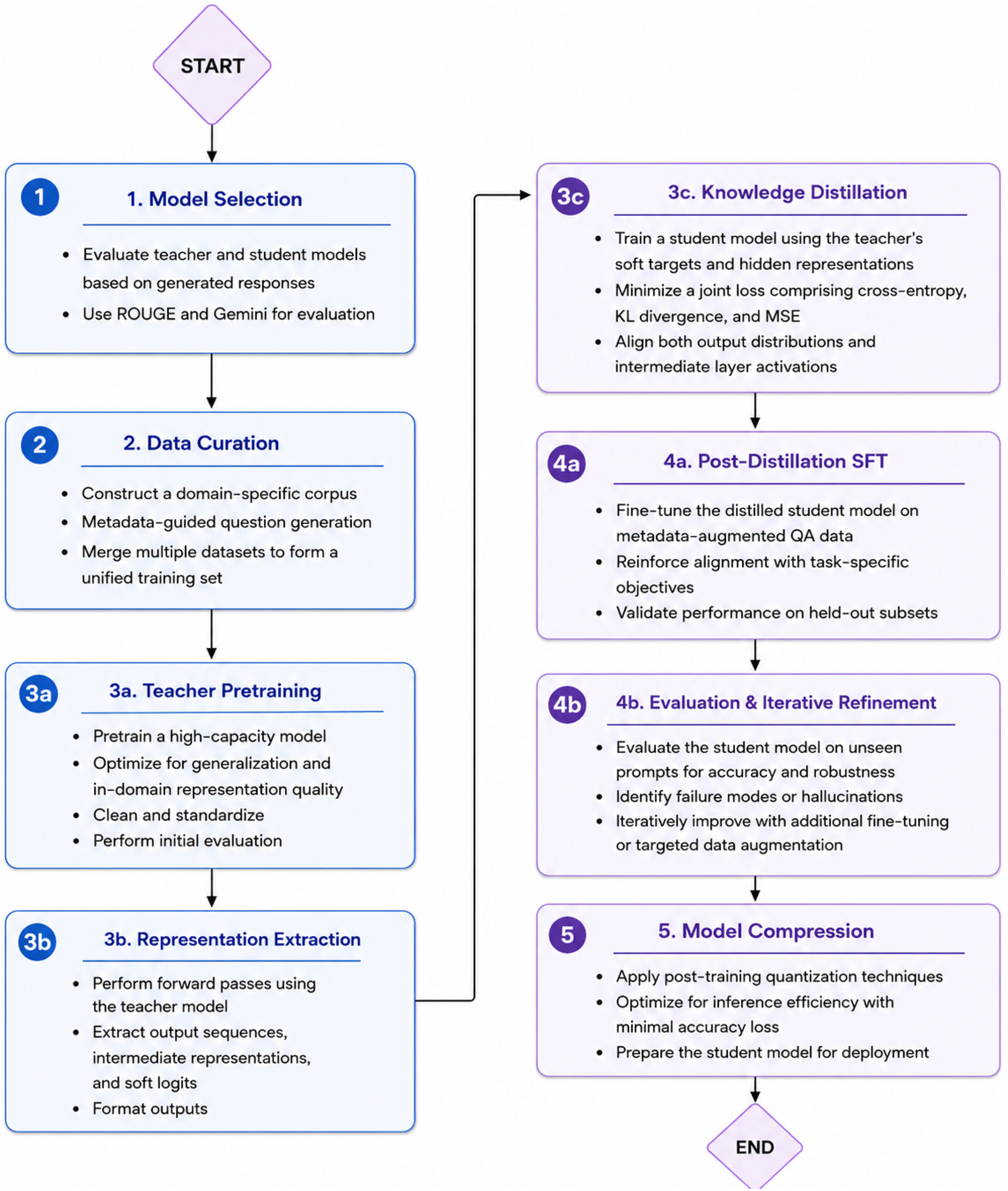
Our approach follows a five-stage pipeline: (1) teacher and student model selection, (2) domain-specific data curation, (3) knowledge distillation with feature transfer, (4) post-distillation supervised fine-tuning (SFT), and (5) model compression and quantization. Figure 1 shows the complete workflow, including evaluation. We describe each stage in the subsections that follow.
4.1. Model Selection
Model selection sets the upper bound on the quality attainable by the student. The teacher’s capacity directly influences the knowledge available for transfer, consistent with the observation that larger, more capable teachers tend to provide better guidance during distillation [8,9].
4.1.1. Teacher Model Selection
We shortlisted twelve open-source transformer LLMs from the Hugging Face Hub as teacher candidates: LLaMA3.1-8B-Instruct [34], LLaMA3-8B-Instruct [33], LLaMA3.2-3B-Instruct [35], Qwen2.5-7B-Instruct and Qwen2.5-3B [36], Qwen3-4B and Qwen3-1.7B [37], Qwen2-1.5B [38], Mistral-7B-Instruct [39], Yi-1.5-6B-Chat [40], Gemma-2B [41], and Phi-2 [42]. Candidates were chosen for computational tractability and adaptability to industrial metrology tasks, with a focus on demonstrated generalization across technical domains, since architecture affects domain-adaptation performance [24]. To evaluate each candidate, we sampled a random subset of 100 prompts from a master pool of 3,000 domain-specific CMM prompts spanning diagnostic procedures, calibration workflows, and metrological interpretations. The same 100-prompt subset was used for every candidate, so that the comparison is consistent across models.
We scored model outputs along three dimensions: factual accuracy, domain relevance, and linguistic coherence. Because ROUGE alone cannot capture the semantic nuances of technical metrology, we adopted an “LLM-as-a-judge” protocol to assess reasoning and accuracy, a practice that has been validated for technical domains [25]. The judge was Gemini 2.0 Flash [32], accessed via API using its default decoding settings (no custom temperature, top-p, or system configuration). For each item the judge received the original question, the generated response, and the reference response, together with the three weighted criteria (factual accuracy 40%, domain relevance 40%, linguistic coherence 20%), and was instructed to return a single integer Gemini Score on a 1–10 scale; the criterion weighting was therefore applied by the judge itself rather than computed post hoc. The judge prompt also instructed the model to penalize hallucinated or unsupported technical claims within the factual-accuracy component. The full generation and evaluation prompts are reproduced verbatim in Appendix A.2. We note that this evaluation used a single judge model and a single scoring pass; reliability concerns arising from the use of a proprietary judge and the absence of repeated runs are discussed explicitly in Section 6.7. In addition, ROUGE scores were computed against expert-style ground-truth responses to quantify lexical overlap [26]: ROUGE-1 (unigram), ROUGE-2 (bigram), and ROUGE-L (longest common subsequence).
Final rankings combined the ROUGE scores into a single composite,
which was then merged with the semantic judge score:
The 0.7/0.3 weighting in Equation (13) is a deliberate design choice that prioritizes semantic quality over lexical conformity because, in technical metrology, a response can be lexically close to a reference yet semantically incorrect, or lexically different yet still correct. We use a simple convex linear combination for interpretability, as it makes the relative contribution of each term transparent. We acknowledge that alternative aggregation schemes exist, such as rank-based aggregation, a harmonic mean that penalizes weakness in either term, or a learned combiner, and that we did not perform a systematic comparison among them. The chosen weights should therefore be interpreted as a transparent reporting convention rather than an optimized objective.
4.1.2. Student Model Selection
We evaluated eight compact models as student candidates using the same 100-prompt benchmark: Qwen3-0.6B [37], Qwen2.5-0.5B and Qwen2-0.5B [36,38], Phi-1.5 [42], TinyLlama-1.1B [43], Falcon-RW-1B [44], GPT-Neo-1.3B [45], and DistilGPT-2 [46]. Here the focus was on baseline capability-to-efficiency ratio before distillation. We restricted the search to architectures under 2B parameters, so as to support a low-footprint, on-premise deployment and the sub-second response times needed for edge integration without external APIs.
4.2. Domain-Specific Data Curation
Effective domain adaptation requires high-quality, contextually rich data. We used a hybrid strategy that combines synthetic generation with real-world extraction [3]. Synthetic prompt-response generation drew on several high-performing LLMs, namely the systems behind ChatGPT [10], Claude [12], Gemini [11], and DeepSeek [15], in order to reduce single-model bias and increase response diversity [4].
These models were prompted with a standardized instruction template covering diagnostic procedures, calibration workflows, and metrological interpretation. The system prompt instructed the model to restrict itself to established CMM facts, to avoid fabricating specifications, values, error codes, tolerances, or ISO clauses, and to state uncertainty explicitly rather than invent details (the full prompt is reproduced in Appendix A.2). To keep generated data aligned with ground-truth technical specifications, we used a few-shot prompting strategy with manually designed prompt–response pairs as semantic anchors. We then performed document parsing on ISO-compliant calibration records, operating manuals, and inspection logs, using domain-specific regular expressions and natural language processing (NLP) filters to extract and clean actionable text. Finally, we applied a metadata-guided question-and-answer (Q&A) generation strategy with the teacher model. High-level CMM topics, such as error handling, component behaviour, calibration protocols, and usage patterns, served as seeds for domain-specific system prompts that generated additional synthetic Q&A pairs.
4.3. Validation Procedure and Its Statistical Effect
All generated and parsed samples were manually reviewed internally by the authors’ research team. Reviewers checked each candidate sample for three properties: factual correctness against the source specification, terminological consistency with CMM/ISO usage, and procedural validity (whether the described steps are coherent and correctly ordered). Samples failing any check were rejected. We state plainly that this validation was performed by the project team rather than by independent, external metrology experts, and that we did not compute a formal inter-rater reliability statistic; this is a limitation (Section 6.7). The overall acceptance rate was 88% (see Table 3), meaning that roughly 12% of generated candidates were removed. Because rejection targeted hallucinated specifications, off-domain drift, and terminologically inconsistent text, the filtering systematically shifts the retained corpus toward higher domain relevance and tighter terminology, at the cost of some lexical and stylistic diversity in the tails of the distribution. We did not quantify this distributional shift directly (e.g., via embedding-space density estimates), and we note it as a candidate for future analysis.
4.4. Knowledge Distillation and Feature Transfer
To compress knowledge from the teacher into the student, we used a multi-stage knowledge distillation (KD) framework [8] that aligns features at more than one level: it transfers signal from the final output layer (logits) and from the final-layer hidden state, so that the student learns both the teacher’s predictions and an aligned internal representation.
4.4.1. Knowledge Distillation Process
KD begins with response generation for the curated prompts. The teacher processes each synthetic CMM prompt to produce a response together with its top-k logits, the corresponding token indices, and its final-layer hidden states. These artifacts are stored offline and then used to train the pre-trained student, allowing it to acquire domain knowledge under teacher guidance while retaining its general capabilities.
4.4.2. Feature Extraction
We extracted two teacher features. First, top-k logits were retained per generation step; k was chosen to capture the large majority (approximately 95–99%) of the probability mass while bounding storage, exploiting the heavy-tailed nature of language-model output distributions [27]. Second, the final-layer hidden state was retained to encode task-relevant semantics. Because of the memory cost of storing and aligning intermediate representations on the target hardware, we restricted hidden-state alignment to the final layer; matching only the final layer can still yield strong student performance under resource constraints [28].
4.4.3. Cross-Tokenizer Logit Alignment and Sparse KL
A key challenge arises when teacher and student do not share a tokenizer or vocabulary, as is the case for our LLaMA3.1-8B teacher and Qwen2-0.5B student. The two models index their vocabularies differently, so the teacher’s top-k logit indices cannot be applied directly to the student’s output. We resolve this with a string-level remapping. For each retained teacher token index, the token is decoded to its surface string with the teacher tokenizer and then re-encoded with the student tokenizer. Only teacher tokens that map to exactly one student token are retained; tokens that decode to an empty string, or that re-encode into multiple student sub-tokens, are discarded, because they cannot be placed in unambiguous one-to-one correspondence. When two distinct teacher tokens map to the same student token, the entry with the larger logit is kept. For each generation step, this procedure produces a set of student vocabulary indices with associated teacher logits, defined over a shared support.
Crucially, the KL divergence is computed over this shared support, not over a reconstructed full-vocabulary vector. The teacher distribution is a temperature-scaled softmax over the retained teacher logits, and the student distribution is obtained by gathering the student logits at the same indices and applying a temperature-scaled log-softmax over that restricted set:
Restricting both distributions to means that no probability mass is assigned to non-top-k tokens on either side, which avoids the distortion that can occur when an unobserved full-vocabulary target is reconstructed from a zero-initialized vector. For the same-architecture Qwen2.5-7B/Qwen2.5-0.5B pair, the tokenizers coincide, so the remapping reduces to an identity map and Equation (14) applies with no token loss. For the cross-architecture pair, the discard rule, which drops multi-token and unmappable entries, reduces the effective support per step. We view recovering this lost signal, for example through learned vocabulary alignment, as a direction for future work.
4.4.4. Training Procedure
The student is trained with the composite loss in Equation (6), with weights , , and . These weights prioritize task performance (cross-entropy), give substantial weight to behavioural mimicry (KL), and assign moderate weight to representation alignment (hidden state) [9]. The weights were selected by a coarse grid search on a held-out validation split; we did not produce dense per-coefficient sensitivity curves, and a systematic sensitivity analysis over is left to future work (Section 6.7).
4.5. Post-Distillation Supervised Fine-Tuning
After distillation, the student was fine-tuned on the metadata-guided Q&A pairs using cross-entropy loss. To prevent data leakage, the train–test split was performed on the master dataset before any training, distillation, or SFT. This two-phase structure lets the student retain the general knowledge transferred during distillation while sharpening task-specific accuracy on the augmented synthetic data, improving factual alignment and reducing domain errors.
4.6. Model Compression and Quantization
For deployment on memory-constrained systems, the distilled model was quantized with GPTQ [21], a post-training method that limits degradation using second-order (Hessian-based) weight information and permits accurate low-bit quantization without retraining. A domain-specific calibration set of 300 prompts, randomly sampled from the curated training data, was used during quantization to preserve generation quality in the target domain. To avoid skewing calibration toward any single topic, the 300 prompts were drawn so as to span the curated topic categories (diagnostics, calibration, component behaviour, error handling), preserving lexical and topical coverage and thereby supporting out-of-distribution robustness on related but unseen phrasings; selection was by stratified random sampling across these categories rather than by a learned criterion. The 4-bit variant was produced with AutoGPTQ, yielding a 700 MB model. In a parallel experiment, the Qwen2-0.5B student was quantized to 8-bit, yielding a 500 MB model for the most constrained environments [23].
4.7. Deployment Strategy
The quantized models were tested across a range of hardware: consumer laptops with an Intel Core i5 (11th gen, octa-core) and 8 GB RAM, CPU-only virtual machines, and GPU-enabled cloud instances. Optimized backends, particularly llama.cpp [7], were used to maximize CPU efficiency and minimize latency, enabling deployment without specialized GPUs while keeping sub-second responses for typical single CMM queries and adhering to a 30-second timeout when batch processing 20–30 questions per document. Latency was measured using time to first token (TTFT).
4.8. Security Considerations
To limit IP leakage and misuse, we adopted a semi-open deployment: only quantized binaries were released publicly, while internal checkpoints and prompt templates were kept private.
5. Experiments and Results
This section evaluates the development of compact, domain-aligned LLMs for CMM operations. Our aim is to test whether specialized metrological knowledge can be compressed from high-parameter teachers into lightweight students without an unacceptable loss of technical accuracy. We state at the outset that all reported values are single-run point estimates: each configuration was trained and evaluated once, and we therefore do not report confidence intervals, multiple-seed averages, or significance tests. We make this explicit so that the magnitudes below are read as indicative single-run measurements rather than as variance-controlled estimates; differences of a few tenths of a Final Score point should be interpreted with corresponding caution. As a partial step toward addressing this, Section 5.7 reports a seed-varied re-evaluation of the deployed model and its baseline, with across-seed dispersion and a bootstrap confidence interval; a full multi-seed re-evaluation of all pipeline stages remains required follow-up work (Section 6.7).
5.1. Teacher Model Selection Results
We evaluated all twelve candidates, each on the random 100-prompt subset drawn from the 3,000-prompt master pool. Table 1 presents the results.
Figure 2.
Performance distribution of teacher model candidates.
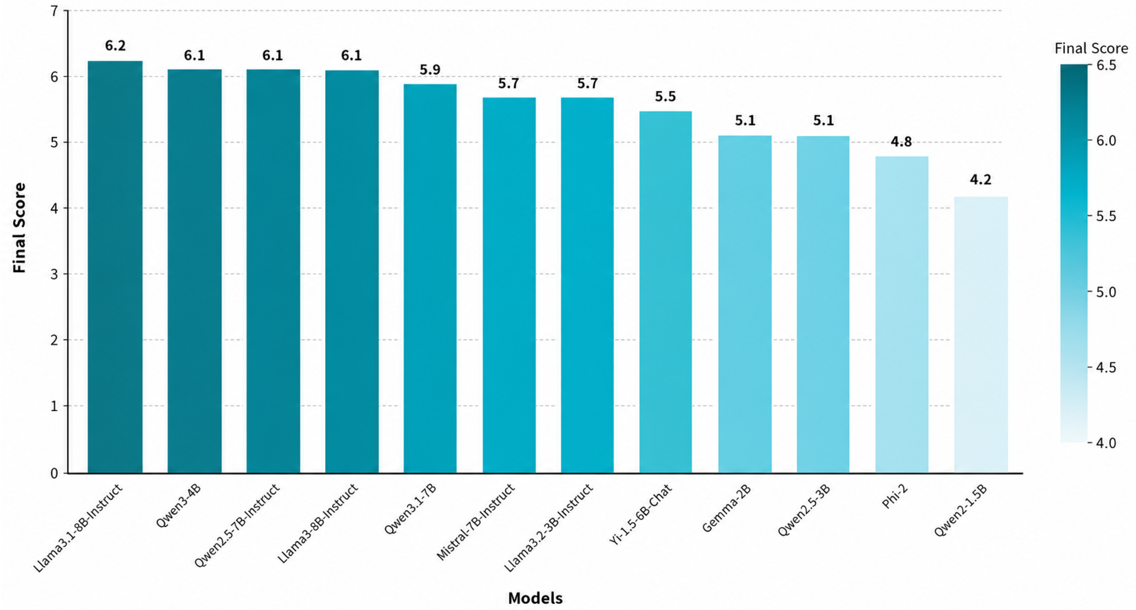
LLaMA3.1-8B-Instruct was the top candidate, with a Final Score of 6.2 and the highest Gemini Score (8.16), reflecting a strong balance of lexical and semantic quality. The Qwen family was consistent across scales, with Qwen3-4B and Qwen2.5-7B-Instruct tied at 6.1. Overall, larger instruction-tuned models tended to score higher.
5.2. Student Model Selection Results
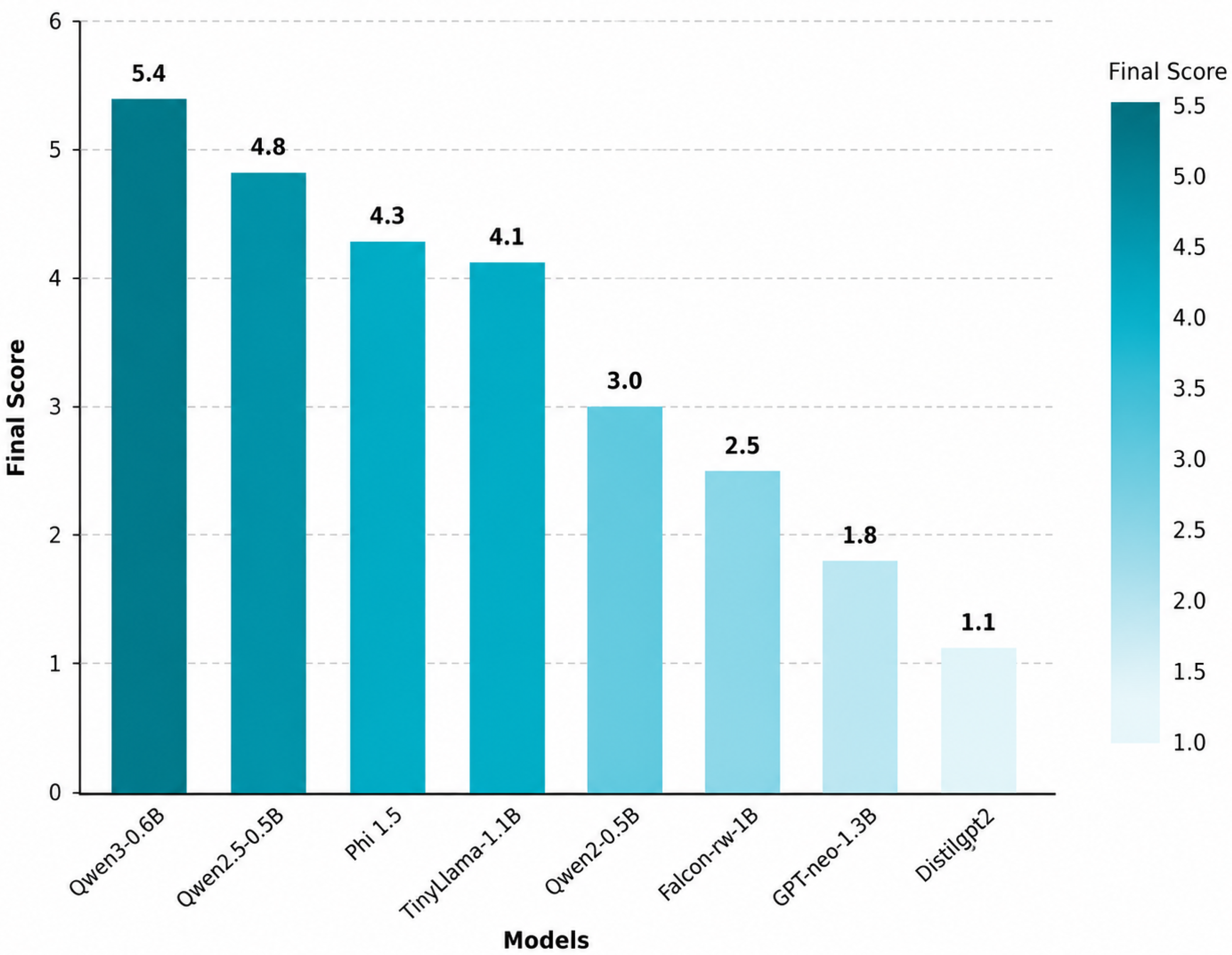
We evaluated eight compact models as students on the same benchmark, targeting 0.5B–1.5B parameters for resource-constrained deployment. Table 2 reports their baseline performance.
Qwen3-0.6B had the best baseline (Final Score 5.4). Smaller models degraded notably, especially in Gemini Score. While Qwen3-0.6B was strongest on raw benchmark score, the final student choice also weighed architectural compatibility and deployment feasibility, as detailed in Section 5.3.
Figure 3.
Baseline performance of student model candidates.
5.3. Final Model Selection
We selected two teacher–student pairs on the basis of evaluation metrics and deployment feasibility. The first pairs LLaMA3.1-8B-Instruct (teacher) with Qwen2-0.5B (student), motivated by the teacher’s strong lexical and semantic scores and the student’s compact, instruction-following profile [38]. The second pairs Qwen2.5-7B-Instruct (teacher) with Qwen2.5-0.5B (student), motivated by within-family consistency and a shared tokenizer/architecture, which enables direct hidden-state and logit alignment [36]. Although Qwen3-0.6B had a higher standalone baseline, we prioritized tokenizer/architecture compatibility with the chosen teachers, because a shared (or cleanly mappable) vocabulary is what makes the logit-alignment objective in Section 4.4.3 well posed; the two selected pairs therefore serve as a same-family case and a cross-family case for studying transfer. We did not run a controlled head-to-head distillation of Qwen3-0.6B against the selected students, so this selection rationale is qualitative; a quantitative comparison is left to future work.
5.4. Domain-Specific Data Curation Results
The corpus was built through four channels:
- Few-shot semantic anchoring: manually designed prompt–response pairs used as anchors to preserve factual integrity during generation.
- Technical document parsing: 300 high-quality procedural samples extracted from ISO-compliant calibration records, manuals, and inspection logs via regex and NLP filters.
- Metadata-guided augmentation: 600 additional Q&A pairs generated with the selected teacher (sampling temperature 1.5–2.0 for lexical variety), seeded by high-level metadata topics to cover critical edge cases.
This produced a unified master dataset of 3,900 samples. Every entry was manually reviewed by the research team (Section 4.2), with an overall acceptance rate of 88% and a mean domain-relevance score of 8.9/10 (Table 3).
5.5. Ablation Study: Loss Component Analysis
To assess the multi-objective loss, we ran an ablation on the Qwen2.5-0.5B student (Table 4). The “Baseline (No Distillation)” and “ only” rows also serve as our internal non-distilled and SFT-only reference points, respectively.
The ablation indicates that: (i) logit-based distillation () adds +0.97 points over baseline; (ii) hidden-state alignment adds a further +0.23 points (+2.3% relative), suggesting that internal feature matching helps beyond output-level mimicry; and (iii) the full loss performs best. We caution that the +0.23 gain is a single-pair, single-run result.
5.6. Knowledge Distillation Results
Each student was tested on a held-out set of 200 previously unseen samples, including challenging prompts. Table 5 and Table 6 report the pipeline results. The “Model Stage” column tracks the progression: Student Pretrained (off-the-shelf), Student + Distillation (multi-objective loss, Equation (6)), Student + Distillation + SFT (final full-precision model), and Student + Distillation + SFT + Quantization (deployed model).
For the Qwen2.5 pair, the student was trained for 5 epochs with early stopping, a learning rate of 2e-5 with cosine annealing, batch size 2, and 4 gradient-accumulation steps; performance stabilized after the third epoch. The full-precision model (distillation + SFT) retained 96.1% of the teacher Final Score (6.15 vs. 6.40). After 4-bit quantization, retention was 85.9% (5.50 vs. 6.40).
Figure 4.
Final Score progression through the distillation pipeline for the Qwen2.5 pair.
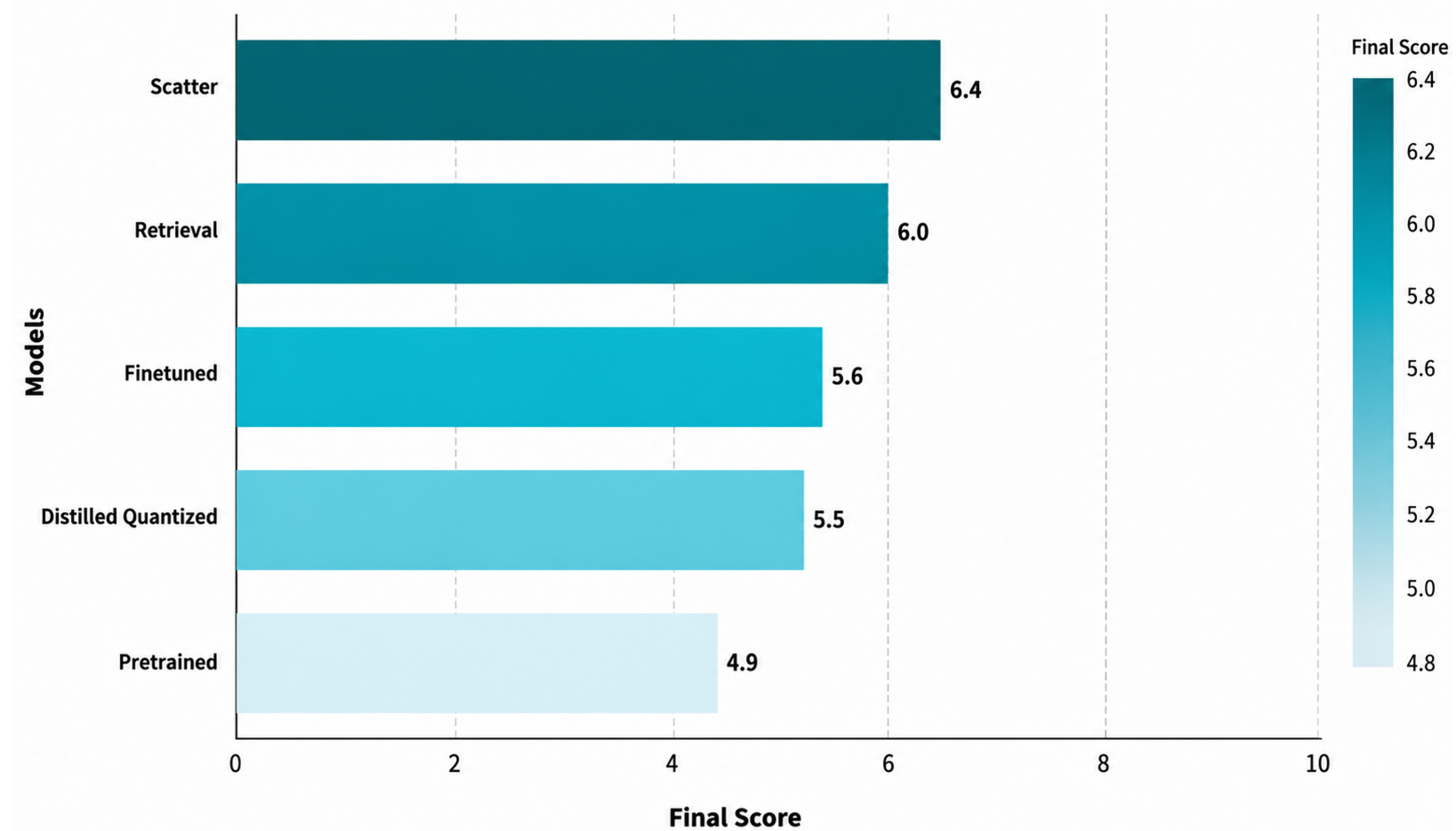
Figure 5.
Final Score progression for the LLaMA3.1/Qwen2 pair. Despite cross-architecture transfer, the student retains 93.4% of teacher performance in full precision.
Figure 5.
Final Score progression for the LLaMA3.1/Qwen2 pair. Despite cross-architecture transfer, the student retains 93.4% of teacher performance in full precision.
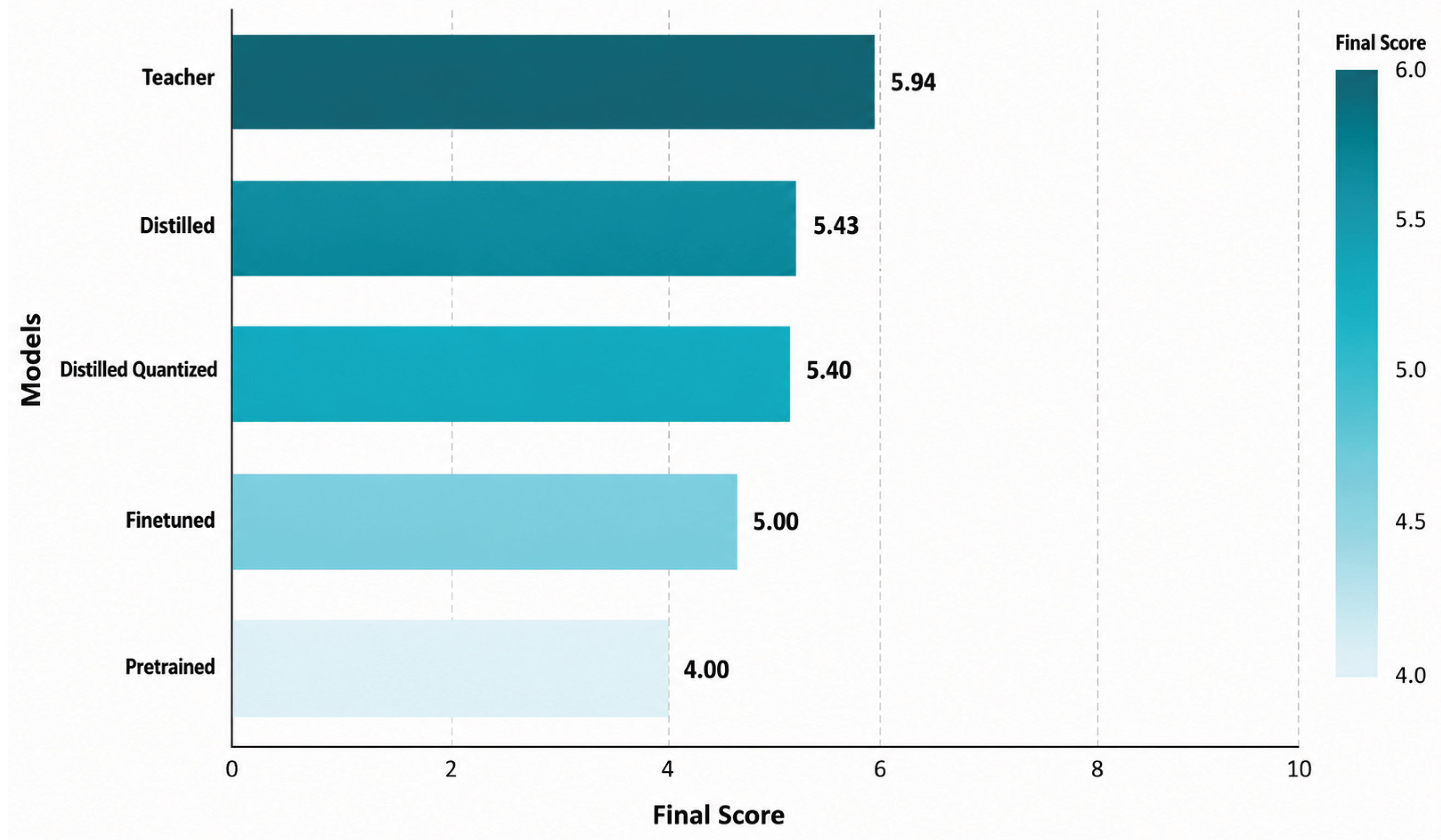
The LLaMA3.1/Qwen2 pair followed a similar regime. The full-precision model (distillation + SFT) retained 93.4% of the teacher Final Score (5.55 vs. 5.94). After 8-bit quantization, retention was 90.9% (5.40 vs. 5.94), indicating effective cross-family transfer via the alignment in Section 4.4.3, with limited degradation from 8-bit quantization.
- Note on lexical metrics exceeding the teacher.
The students’ ROUGE scores (e.g., R-1 ≈ 0.31–0.35) exceed those of their teachers (R-1 ≈ 0.16) even though the teachers receive higher semantic (Gemini) scores. This is expected rather than anomalous. ROUGE rewards surface n-gram overlap with the reference, and the students were fine-tuned directly on the in-domain Q&A distribution, so they reproduce the concise, templated phrasing of the reference answers closely. The teachers, by contrast, produce longer, more elaborated, and more varied responses that are often more informative yet share fewer exact n-grams with the short references, lowering their ROUGE. In other words, high ROUGE here reflects lexical conformity to the reference style, not superior diagnostic quality, which is precisely why the Final Score weights the semantic judge above ROUGE (Equation (13)) and why we do not treat the students’ higher ROUGE as evidence that they surpass their teachers.
5.7. Robustness Check: Seed-Varied Re-Evaluation of Deployed Models
The main pipeline results reported in Table 5 and Table 6 are single-run point estimates, which limits the statistical confidence that can be placed on small inter-stage differences. To address this limitation in part, we conducted a seed-varied re-evaluation of the two final deployed configurations, namely the quantized Qwen2.5 student and the quantized LLaMA/Qwen2 cross-architecture student, together with their respective pretrained baselines. Each configuration was evaluated independently under three random seeds (42, 43, and 44), and the held-out test set was expanded from 200 to 300 prompts per seed, yielding 900 inferences per model configuration across the full re-evaluation.
5.7.1. Evaluation Harness
Owing to the deprecation of the Gemini 2.0 Flash judge used in the main experiment, this re-evaluation employed gemini-3-flash with an identical scoring prompt (Appendix A.2). Because a change of judge model introduces a systematic shift in absolute score magnitude, the results below should not be compared numerically to the main tables; rather, conclusions are drawn from (i) the within-run separation between the deployed model and its pretrained baseline under the same judge, and (ii) the across-seed dispersion of each configuration. ROUGE scores are computed locally using standard tokenization and are therefore directly comparable across all tables.
5.7.2. Results
Table 7 presents per-seed scores and seed-averaged statistics for both evaluation pairs. For each pair, the deployed (distilled + SFT + quantized) model is listed first, followed by its pretrained baseline.
5.7.3. Lexical Stability
This low dispersion holds for both the deployed models and their pretrained baselines. Because the across-seed standard deviation (0.003) is smaller than the deployed-vs-baseline ROUGE gap in both pairs, the lexical difference between the deployed model and its pretrained baseline is unlikely to be a seed-sampling artefact, though we did not perform a formal significance test.
5.7.4. Semantic Improvement and Cross-Seed Consistency
For the native Qwen2.5 pair, the deployed model achieves a mean Final Score of against a pretrained baseline of , a consistent margin of points across all three seeds. The corresponding mean Gemini Score rises from to , a -point gain in semantic quality attributable to distillation, supervised fine-tuning, and quantization. The narrow standard deviations confirm that this improvement is reproducible rather than an artefact of a single evaluation run. For the cross-architecture LLaMA/Qwen2 pair, the deployed model attains a mean Final Score of against a pretrained baseline of , a margin of points. The Gemini Score rises from to , an improvement of points, demonstrating that cross-family knowledge transfer via the string-level logit-alignment procedure described in Section 4.4.3 yields robust and reproducible gains even in the presence of heterogeneous tokenizers. The per-seed Gemini Scores for this pair (6.62, 6.74, 6.65) are closely clustered, with a standard deviation of 0.06, further reinforcing the stability of the cross-architecture transfer.
5.7.5. ROUGE Behavior
The deployed Qwen2.5 student shows a marginal decrease in ROUGE relative to its pretrained baseline ( vs. ), which mirrors the pattern observed in the main pipeline tables and is discussed there: fine-tuning shifts the student toward more elaborated, semantically richer responses that share fewer exact n-grams with the concise reference answers, even as semantic quality improves. This highlights the importance of the judge-weighted Final Score as the primary evaluation criterion. For the cross-architecture pair, ROUGE increases modestly after distillation ( vs. ), reflecting improved alignment with the reference response style transferred from the LLaMA teacher.
5.7.6. Scope of This Check
We emphasize that this robustness analysis covers only the final deployed configurations (distill + SFT + quantization). The intermediate pipeline stages (distillation only; distillation + SFT without quantization) were not re-evaluated across seeds, because the corresponding checkpoints were not retained after the main experiment. A comprehensive multi-seed evaluation spanning all pipeline stages, conducted under a fixed and reproducible judge, remains the most important methodological follow-up and is listed explicitly in Section 6.7.
5.8. Post-Distillation Fine-Tuning Impact
Post-distillation SFT improved both students (Table 8).Error analysis across both fine-tuned students showed reductions in three categories: calibration procedures (18.2% → 9.1%), measurement interpretation (15.6% → 8.3%), and diagnostic recommendations (21.4% → 12.7%). These error categories are measured on the held-out set; given its size (200 samples), the absolute rates should be read as indicative rather than definitive.
5.9. Model Compression and Quantization Results
The primary Qwen2.5 student was quantized to 4-bit (Table 9); the LLaMA3.1/Qwen2 student was quantized to 8-bit (Table 10). Inference speed is reported as TTFT in ms/token.We deliberately report memory compression and inference speedup as separate quantities rather than a single “efficiency gain,” because they measure different things: quantization reduced model size by about 75% (a 4.0× memory-compression ratio at the model level), while TTFT improved by a more modest 1.58–1.62×. The larger memory-compression ratios cited elsewhere in this paper (21.4×, 32×) are teacher-to-quantized-student comparisons and reflect parameter-count reduction plus quantization, not end-to-end inference speedup. 8-bit quantization retained more performance (97.3%) than 4-bit (89.4%), so the bit-width can be chosen per hardware constraint. We did not directly measure energy consumption; any reduction in power draw is expected from the smaller memory footprint and lower precision, but is not quantified here.
5.10. Deployment Validation Results
Multi-tier hardware validation (Table 11) reports RAM usage, TTFT, and a success rate, where “success” denotes completion of the query within the configured timeout and without runtime error. We did not separately log sustained tokens/second, end-to-end response time at fixed context length, peak CPU utilization, or power, and we flag these as missing deployment metrics in Section 6.7.
5.11. Comparative Analysis
Comparing teachers against their final distilled-and-quantized students shows large memory compression with strong performance retention (Table 12, Table 13 and Table 14).
5.11.1. Positioning Relative to Other Compression Approaches
Our experiments compare pipeline stages against each other (pretrained → distilled → SFT → quantized) and include non-distilled and SFT-only reference points via the ablation (Table 4). We did not run external baselines such as LoRA/QLoRA fine-tuning of the same small students [23,29], retrieval-augmented generation (RAG) over the CMM corpus [30], or alternative compression methods, primarily because of compute constraints during the revision period. We therefore refrain from claiming superiority over these approaches; a controlled comparison against LoRA/QLoRA and a local RAG system on identical hardware and the same test set is an important and explicitly planned next step.
6. Discussion
6.1. Key Findings
We performed knowledge distillation for two model pairs. The Qwen2.5 student reached 96.1% of its teacher’s Final Score (full precision) with roughly 15× fewer parameters; the LLaMA3.1/Qwen2 student reached 93.4% with roughly 16× fewer parameters via cross-family transfer. The ablation suggests that hidden-state alignment contributes about +2.3% over logit-only distillation on the tested pair. Post-distillation SFT added 2.2–2.5% and reduced domain-specific error rates. Quantization confirmed deployment viability: 8-bit introduced a small drop (2.7%), while 4-bit maximized compression with a larger drop (10.6%). Together, these results indicate practical feasibility for constrained settings, while the caveats below bound how far the claims should be taken.
6.2. Robustness on Complex Diagnostics and Quantization
The quantization drops in Section 5.9 are aggregate figures over the held-out set. We expect the 4-bit performance drop to be unevenly distributed. Routine, frequently encountered queries are likely to be affected the least, whereas complex, multi-step, or non-routine maintenance diagnostics, which depend on precise numerical reasoning and longer chains of inference, are the most likely to experience degradation. We did not separately stratify performance by diagnostic complexity, so this expectation remains a hypothesis rather than a measured result. Stratified evaluation by failure mode and routine versus non-routine status is therefore needed to confirm it.
6.3. Deployment Boundaries on Embedded Hardware
The edge-device row in Table 11 (ARM CPU, 4 GB, 52 ms/token, 95% success) already shows the cost of constrained hardware. On older embedded platforms without high-bandwidth memory or large caches, decode is bandwidth-bound: each token requires streaming the model weights through limited memory bandwidth, so latency is dominated by memory traffic rather than arithmetic. On such platforms the 500–700 MB quantized footprint may still exceed comfortable working-set limits, leading to cache thrashing and degraded throughput. Reliable deployment on sub-4 GB embedded targets therefore likely requires further reduction (e.g., lower-bit or mixed-precision quantization, weight pruning, or smaller students), and we do not claim that the current binaries run acceptably on arbitrary legacy embedded hardware.
6.4. Hallucination Risk and Operator Safety
As discussed in Section 1, autoregressive generation can propagate an early error through an entire response, and a confidently phrased but incorrect diagnostic could mislead an operator. This is the central safety vulnerability of the approach. At the prompt level we applied two mitigations: the response-generation system prompt instructed the model to avoid fabricating specifications and to express uncertainty, and the judge prompt penalized hallucinated or unsupported claims (Appendix A.2). These are soft, prompt-level controls only: they were not separately measured, they do not guarantee abstention, and a model can still produce confident errors despite such instructions. We did not implement or evaluate stronger hallucination-resistance mechanisms (e.g., calibrated abstention/uncertainty signalling, retrieval grounding against source manuals, or constrained decoding over an approved action vocabulary), and we recommend that the system be used strictly as an operator-in-the-loop aid rather than an authority. Adding and evaluating such safeguards is necessary before any safety-critical use.
6.5. Operational Updates Without Catastrophic Forgetting
Industrial standards and operating guides change over time, so a deployed model must be updatable without losing prior competence. We outline a proposed update routine for future work rather than a validated procedure: (i) maintain a versioned, append-only corpus of validated CMM samples; (ii) when a standard or manual is revised, generate and validate a focused delta set covering the changed content; (iii) periodically re-run a lightweight re-distillation or fine-tuning that mixes the delta set with a replay/rehearsal sample of older data to limit catastrophic forgetting; (iv) optionally isolate new-standard knowledge in low-rank adapters [29] that can be attached or detached, keeping the base student stable; and (v) consider regularization such as elastic weight consolidation [31] to protect parameters important to earlier tasks. Each step needs empirical validation, including measuring forgetting on a fixed regression set after each update.
6.6. Implications for Industrial AI
This work demonstrates a workable engineering pipeline for an on-premise, specialist CMM assistant. The resulting model is intended as a secure, embedded aid that could, in principle, be integrated into existing CMM software ecosystems such as Zeiss CALYPSO, Hexagon PC-DMIS, and Maestro CMM stacks, providing localized diagnostic support, error-log interpretation, and procedural guidance at the control console without an internet connection. We stress that such integration is a design possibility we have not demonstrated: we did not run interface-level integration, API tests, operator-workflow studies, or production trials, so claims of plug-in readiness for any specific vendor stack would be premature.
The approach offers two operational benefits in principle. First, proprietary intellectual property (IP), such as part schematics, measurement routines, and internal quality data, can remain on-premise, reducing the exposure associated with cloud APIs. Second, it trades recurring per-token API costs for a largely one-time training cost, and the measured on-premise latency (34–38,ms/token TTFT on consumer hardware) provides a responsive baseline for operators. Beyond CMMs, the same on-premise specialist pattern may be applicable to other sensitive, knowledge-intensive settings, for example CNC machining diagnostics, robotic assembly fault detection, and broader quality control, as well as regulated fields such as medical, financial, and legal document workflows. We present these as plausible extensions to be tested rather than as established outcomes.
6.7. Limitations and Future Work
We summarize the study’s main limitations below.
- Synthetic-data dependence and circularity. A large share of training data was generated by LLMs and the semantic judge is also an LLM, which raises the risk of teacher-induced bias, hallucinated domain knowledge, and inflated metrics. Few-shot anchoring, document parsing, and manual review mitigate but do not eliminate this; incorporating more authentic CMM logs, calibration cases, maintenance records, and expert-verified troubleshooting cases is a priority.
- Validation rigor. Sample validation was performed internally by the research team, without independent external metrology experts and without a formal inter-rater reliability measure.
- Evaluation protocol. The Final Score relies heavily on a proprietary judge (Gemini 2.0 Flash, default settings) and on ROUGE. We did not separately measure factual correctness against authoritative sources, ISO-clause compliance, hallucination resistance, or the safety of troubleshooting recommendations, and we did not assess judge self-consistency across repeated runs or prompt variants.
- Statistical rigor. The main pipeline results (Table 5 and Table 6) are single-run point estimates; because the gaps between adjacent pipeline stages are sometimes only a few tenths of a Final Score point, they should not be read as statistically established. As a partial mitigation, Section 5.7 reports a seed-varied re-evaluation of the deployed model and its baseline, showing low across-seed ROUGE dispersion and a bootstrap confidence interval for the deployed model’s judge score. We were unable to extend this to a full multi-seed, all-stage re-evaluation for three reasons: the intermediate checkpoints (distillation-only and distillation+SFT, prior to quantization) were not retained and would require re-training to re-score; the original LLM judge was deprecated, so any re-run relies on a different judge whose absolute scores are not comparable to the main tables; and re-scoring under a replacement judge is constrained by API budget, which additionally left the deployed model’s judge evaluation complete for only one of the three seeds. Full seed-averaged evaluation with per-stage dispersion and significance testing, ideally against a fixed and reproducible judge, remains the most important methodological follow-up.
- Test-set size and coverage. The held-out set has 200 samples. Given the safety-critical context, larger and more diverse test sets are needed, covering multiple industrial scenarios, unseen machine types and failure modes, and expert-blind evaluation.
- Missing external baselines. We did not compare against LoRA/QLoRA-tuned small models, local RAG systems, or other compression baselines (compute-constrained during the revision); controlled comparisons are planned.
- Cross-architecture coverage loss. The string-level logit remapping discards multi-token and unmappable teacher entries, shrinking the effective top-k support in the cross-family pair; recovering this signal is open.
- Single-pair ablation. The hidden-state-alignment ablation was run only on the Qwen2.5 pair; its contribution should be re-tested across additional architectures.
- Deployment metrics. We reported TTFT, RAM usage, and success rate, but not sustained tokens/second, end-to-end response time at fixed context length, peak CPU utilization, or power.
- Integration not demonstrated. Compatibility with specific vendor software stacks was not tested at the interface or workflow level.
- Hyperparameter sensitivity. The loss weights were set by a coarse grid search; dense sensitivity curves were not produced.
- Quantization trade-off. 4-bit causes a 10.6% drop for the Qwen2.5 pair versus 2.7% at 8-bit for the LLaMA/Qwen2 pair; mixed-precision or query-adaptive quantization may help.
- Language coverage. Evaluation was English-only; multilingual CMM environments are not covered.
7. Conclusions
We presented a five-stage pipeline for building domain-aligned, compact LLMs for CMM operations. The pipeline transferred knowledge from 7.5B- and 8B-parameter teachers to 0.5B-parameter students, retaining 93.4–96.1% of teacher performance in full precision under our composite metric, including a cross-family transfer enabled by a string-level logit-alignment procedure with a support-restricted KL objective. An ablation indicated a small (+2.3%) gain from hidden-state alignment on the tested pair, post-distillation SFT added 2.2–2.5%, and post-training quantization achieved up to a 32× memory-compression ratio (teacher-to-quantized-student) with a more modest inference speedup, while retaining most capability. The final quantized models ran at 34–38 ms/token TTFT on consumer hardware. We position this work as a systems and domain adaptation contribution that integrates established techniques for a privacy-sensitive industrial setting, and we have documented its limitations candidly, most notably its reliance on synthetic data and a proprietary judge, single-run point estimates, a small test set, and the absence of external baselines and field validation. Addressing these limitations is the focus of future work and, in our view, is essential for advancing the approach from a promising prototype to a deployable industrial tool.
Author Contributions
Conceptualization, A.P.; methodology, A.P., M.P.N. and P.S.; software, M.P.N. and P.S.; validation, A.P., M.P.N. and P.S.; formal analysis, M.P.N. and P.S.; investigation, A.P., M.P.N. and P.S.; resources, A.P.; data curation, M.P.N. and P.S.; writing (original draft preparation), A.P.; writing (review and editing), A.P. and Y.S.S.R.M.; visualization, M.P.N. and P.S.; supervision, A.P. and Y.S.S.R.M.; project administration, A.P. All authors have read and agreed to the published version of the manuscript.
Funding
This research received no external funding.
Institutional Review Board Statement
Not applicable.
Informed Consent Statement
Not applicable.
Data Availability Statement
The data and code that support the findings of this study are available from the corresponding author upon reasonable request.
Conflicts of Interest
The authors declare no conflicts of interest.
Abbreviations
The following abbreviations are used in this manuscript:
| LLM | Large Language Model |
| CMM | Coordinate Measuring Machine |
| KD | Knowledge Distillation |
| SFT | Supervised Fine-Tuning |
| PTQ | Post-Training Quantization |
| GPTQ | Generative Pre-trained Transformer Quantization |
| LoRA | Low-Rank Adaptation |
| QLoRA | Quantized Low-Rank Adaptation |
| RAG | Retrieval-Augmented Generation |
| KV | Key-Value |
| TTFT | Time to First Token |
| ROUGE | Recall-Oriented Understudy for Gisting Evaluation |
| MSE | Mean Squared Error |
| OOD | Out Of Distribution |
| AI | Artificial Intelligence |
| GPU | Graphics Processing Unit |
| CPU | Central Processing Unit |
| NVMe | Non-Volatile Memory Express |
| IP | Intellectual Property |
| ISO | International Organization for Standardization |
| GKD | Generalized Knowledge Distillation |
| MoT | Merge-of-Thought |
| API | Application Programming Interface |
| NLP | Natural Language Processing |
| Perf. | Performance |
| Quant. | Quantized |
Appendix A. Additional Experimental Details
Appendix A.1. Quantization and Distillation Settings
- Removing quantization increased latency by roughly 40% and memory footprint by about 4×.
- The temperature for the KL objective was set to 2.0 based on preliminary experiments.
- The projection P in Equation (9) is a learnable linear layer mapping the student hidden dimension to the teacher’s, trained jointly with the student under the mean-squared-error objective.
- The cross-tokenizer logit alignment (Section 4.4.3) decodes each retained teacher token to text and re-encodes it with the student tokenizer, keeping only one-to-one mappings and resolving collisions by maximum logit; the KL divergence is then evaluated over the shared top-k support.
Appendix A.2. Generation and Evaluation Prompts
For reproducibility, we reproduce the two prompts used in the study. The first is the system prompt used to generate teacher and synthetic responses; rules 3–5 constrain the model against fabricating technical content. The second is the prompt used to obtain the Gemini Score; it returns a single integer rating and explicitly penalizes hallucinated claims.
Response-generation system prompt.
You are a precise CMM (Coordinate Measuring Machine) technical expert.
Follow these rules strictly:
1. ONLY provide factual, technical information about CMMs.
2. Start your response directly with the technical information - no
preambles or thinking out loud.
3. Do not fabricate specifications, measured values, error codes,
tolerances, part numbers, or ISO clause numbers; state only
information you can support.
4. If you are uncertain or lack sufficient information to answer
reliably, say so explicitly rather than inventing details.
5. Do not extrapolate beyond established CMM principles; avoid
speculative or unverifiable claims.
6. Keep responses concise, technical, and informative.
7. Focus on general CMM principles and established technical facts.
8. Use plain text only - no markdown formatting.
9. Begin responses immediately with technical content.
Gemini-judge evaluation prompt.
Evaluate the following CMM-related response on a scale of 1-10 based on:
1. Factual accuracy (40%)
2. Domain relevance to CMM operations (40%)
3. Linguistic coherence (20%)
When scoring factual accuracy, heavily penalize hallucinated or
unsupported technical claims (for example invented error codes,
fabricated tolerances or measured values, or non-existent ISO
clauses), even if the response is otherwise fluent and well
structured. A confidently stated but factually unsupported response
should receive a low factual-accuracy contribution.
Original Question: {prompt}
Generated Response: {generated_response}
Reference Response: {reference_response}
Provide only a single number between 1 and 10 as your rating.
References
- Zhu, X.; Li, J.; Liu, Y.; Ma, C.; Wang, W. A Survey on Model Compression for Large Language Models. Trans. Assoc. Comput. Linguist. 2024, 12, 1556–1577. [Google Scholar] [CrossRef]
- Lin, Y.; et al. Towards Privacy-Preserving LLM Inference via Covariant Obfuscation (Technical Report). arXiv. 2024. Available online: https://arxiv.org/abs/2412.06113.
- Wang, Y.; Kordi, Y.; Mishra, S.; et al. Self-Instruct: Aligning Language Models with Self-Generated Instructions. arXiv. 2022. Available online: https://arxiv.org/abs/2212.10560.
- Longpre, S.; Hou, L.; Vu, T.; et al. The Flan Collection: Designing Data and Methods for Effective Instruction Tuning. arXiv 2023, arXiv:2301.13688. [Google Scholar]
- SoulPage IT Solutions. Deploying Large Language Models On-Premise: A Guide for Enterprises. Link. 2025.
- Mosca, A. Cloud vs On-Premises: Which Is the Best Deployment Option for LLMs? In Capgemini; 2024. [Google Scholar]
- Gerganov, G. llama. cpp: Port of LLaMA for Efficient CPU/GPU Inference. 2023. [Google Scholar]
- Hinton, G.; Vinyals, O.; Dean, J. Distilling the Knowledge in a Neural Network. NIPS Deep Learning Workshop, 2015. [Google Scholar]
- Gou, J.; Yu, B.; Maybank, S. J.; Tao, D. Knowledge Distillation: A Survey. Int. J. Comput. Vis. 2021, 129, 1789–1819. [Google Scholar] [CrossRef]
- OpenAI. GPT-4 Technical Report. arXiv. 2023.
- Gemini Team; Google. Gemini: A Family of Highly Capable Multimodal Models. arXiv 2023, arXiv:2312.11805. [Google Scholar]
- Anthropic. The Claude 3 Model Family: Opus, Sonnet, Haiku. Anthropic Model Card, Link. 2024. [Google Scholar]
- Jiang, A. Q.; Sablayrolles, A.; Mensch, A.; et al. Mistral 7B. arXiv. 2023.
- Perplexity, A.I. Perplexity: AI-Powered Answer Engine (commercial service). 2025. [Google Scholar]
- DeepSeek-AI. DeepSeek-V3 Technical Report. arXiv. 2024.
- Bazeley, M. A Pragmatic Introduction to Model Distillation for AI Developers. Labelbox 2024. [Google Scholar]
- DataCamp. LLM Distillation Explained: Applications, Implementation and More. 2024. [Google Scholar]
- Singh, R.; Sarma, M. S. Optimizing Deployment Strategies for Large Language Models. 2025 IEEE Technology and Engineering Management Society Conference - Global (TEMSCON Global), 2025. [Google Scholar] [CrossRef]
- Kwon, W.; et al. Efficient Memory Management for Large Language Model Serving with PagedAttention. arXiv 2023, arXiv:2309.06180. [Google Scholar]
- Sheng, Y.; et al. FlexGen: High-Throughput Generative Inference of Large Language Models with a Single GPU. arXiv. 2023.
- Frantar, E.; Alistarh, D. GPTQ: Accurate Post-Training Quantization for Generative Pre-trained Transformers. arXiv. 2022.
- Lin, J.; et al. AWQ: Activation-aware Weight Quantization for LLM Compression and Acceleration. arXiv 2023, arXiv:2306.00978. [Google Scholar]
- Dettmers, T.; et al. QLoRA: Efficient Finetuning of Quantized LLMs. arXiv 2023, arXiv:2305.14314. [Google Scholar]
- Rogers, A.; Kovaleva, O.; Rumshisky, A. A Primer in BERTology: What We Know About How BERT Works. Trans. Assoc. Comput. Linguist. 2020, 8, 842–866. [Google Scholar] [CrossRef]
- Zheng, L.; et al. Judging LLM-as-a-Judge with MT-Bench and Chatbot Arena. arXiv 2023, arXiv:2306.05685. [Google Scholar]
- Lin, C.-Y. ROUGE: A Package for Automatic Evaluation of Summaries. Text. Summ. Branches Out. Proc. ACL-04 Workshop 2004, 74–81. [Google Scholar]
- Holtzman, A.; Buys, J.; Du, L.; Forbes, M.; Choi, Y. The Curious Case of Neural Text Degeneration. arXiv. 2019.
- Jiao, X.; et al. TinyBERT: Distilling BERT for Natural Language Understanding. arXiv. 2020.
- Hu, E. J.; Shen, Y.; Wallis, P.; et al. LoRA: Low-Rank Adaptation of Large Language Models. arXiv. 2021.
- Lewis, P.; Perez, E.; Piktus, A.; et al. Retrieval-Augmented Generation for Knowledge-Intensive NLP Tasks. In Advances in Neural Information Processing Systems (NeurIPS); 2020. [Google Scholar]
- Kirkpatrick, J.; Pascanu, R.; Rabinowitz, N.; et al. Overcoming Catastrophic Forgetting in Neural Networks. Proc. Natl. Acad. Sci. (PNAS) 2017, 114, 3521–3526. [Google Scholar] [CrossRef]
- Gemini Team; DeepMind, Google. Gemini 2.5: Pushing the Frontier with Advanced Reasoning, Multimodality, Long Context, and Next Generation Agentic Capabilities. arXiv. 2025.
- Meta, A.I. Meta-Llama-3-8B-Instruct. Hugging Face Model Hub. Hugging Face 2024. [Google Scholar]
- Meta, A.I. Meta-Llama-3.1-8B-Instruct. Hugging Face Model Hub. Hugging Face 2024. [Google Scholar]
- Meta, A.I. Meta-Llama-3.2-3B-Instruct. Hugging Face Model Hub. Hugging Face 2024. [Google Scholar]
- Qwen Team; Cloud, Alibaba. Qwen2.5 Model Series. Hugging Face Model Hub. Hugging Face 2024. [Google Scholar]
- Qwen Team; Cloud, Alibaba. Qwen3 Model Series. Hugging Face Model Hub. Hugging Face 2025. [Google Scholar] [CrossRef]
- Qwen Team; Cloud, Alibaba. Qwen2 Model Series. Hugging Face Model Hub. Hugging Face 2024. [Google Scholar]
- Mistral, A.I. Mistral-7B-Instruct-v0.3. Hugging Face Model Hub. Hugging Face 2024. [Google Scholar]
- 01.AI. Yi-1.5-6B-Chat. Hugging Face Model Hub. 2024.
- Google. Gemma-2B. Hugging Face Model Hub. Hugging Face 2024. [Google Scholar]
- Microsoft. Phi-2 and Phi-1.5. Hugging Face Model Hub. 2023. [Google Scholar]
- Zhang, P.; et al. TinyLlama-1.1B-Chat-v1.0. Hugging Face Model Hub. Hugging Face 2024. [Google Scholar]
- Technology Innovation Institute. Falcon-RW-1B. Hugging Face Model Hub. Hugging Face. 2023. [Google Scholar]
- EleutherAI. GPT-Neo-1.3B. Hugging Face Model Hub. Hugging Face 2021. [Google Scholar]
- Face, Hugging. DistilGPT-2. Hugging Face Model Hub. 2019. [Google Scholar]
Figure 1.
Methodology workflow. The teacher is a pre-trained open-source model that may undergo optional domain-specific fine-tuning before distillation.
Figure 1.
Methodology workflow. The teacher is a pre-trained open-source model that may undergo optional domain-specific fine-tuning before distillation.

| Model | ROUGE-1 | ROUGE-2 | ROUGE-L | Gemini Score | Final Score |
|---|---|---|---|---|---|
| Llama3.1-8B-Instruct | 0.2033 | 0.0398 | 0.1858 | 8.16 | 6.2 |
| Qwen3-4B | 0.2181 | 0.0519 | 0.2008 | 7.98 | 6.1 |
| Qwen2.5-7B-Instruct | 0.2144 | 0.0426 | 0.1914 | 7.98 | 6.1 |
| Llama3-8B-Instruct | 0.1824 | 0.0375 | 0.1688 | 8.04 | 6.1 |
| Qwen3-1.7B | 0.1615 | 0.0322 | 0.1514 | 7.90 | 5.9 |
| Mistral-7B-Instruct | 0.1499 | 0.0277 | 0.1410 | 7.70 | 5.7 |
| Llama3.2-3B-Instruct | 0.2016 | 0.0381 | 0.1867 | 7.42 | 5.7 |
| Yi-1.5-6B-Chat | 0.1200 | 0.0173 | 0.1136 | 7.46 | 5.5 |
| Gemma-2B | 0.1585 | 0.0261 | 0.1489 | 6.78 | 5.1 |
| Qwen2.5-3B | 0.1950 | 0.0325 | 0.1769 | 6.60 | 5.1 |
| Phi-2 | 0.1550 | 0.0195 | 0.1443 | 6.28 | 4.8 |
| Qwen2-1.5B | 0.1662 | 0.0250 | 0.1550 | 5.40 | 4.2 |
| Model | ROUGE-1 | ROUGE-2 | ROUGE-L | Gemini Score | Final Score |
|---|---|---|---|---|---|
| Qwen3-0.6B | 0.2055 | 0.0331 | 0.1842 | 7.02 | 5.4 |
| Qwen2.5-0.5B | 0.1148 | 0.0175 | 0.1065 | 6.46 | 4.8 |
| Phi-1.5 | 0.1149 | 0.0157 | 0.1095 | 5.80 | 4.3 |
| TinyLlama-1.1B | 0.1469 | 0.0198 | 0.1387 | 5.34 | 4.1 |
| Qwen2-0.5B | 0.1512 | 0.0248 | 0.1420 | 3.80 | 3.0 |
| Falcon-rw-1B | 0.1342 | 0.0173 | 0.1283 | 3.14 | 2.5 |
| GPT-neo-1.3B | 0.1334 | 0.0147 | 0.1274 | 2.06 | 1.8 |
| DistilGPT2 | 0.0827 | 0.0047 | 0.0781 | 1.34 | 1.1 |
Table 3.
Dataset quality metrics. “Acceptance rate” is the fraction of generated/parsed candidates retained after internal review.
Table 3.
Dataset quality metrics. “Acceptance rate” is the fraction of generated/parsed candidates retained after internal review.
| Data Source | Volume | Acceptance Rate | Domain Relevance Score |
|---|---|---|---|
| Synthetic Generation | 3,000 | 85% | 8.7/10 |
| Document Parsing | 300 | 92% | 9.2/10 |
| Metadata Augmentation | 600 | 88% | 8.9/10 |
| Total Dataset | 3,900 | 88% | 8.9/10 |
Table 4.
Ablation study: impact of loss components on the Qwen2.5-0.5B student.
| Configuration | Final Score | Improvement (points) |
Description |
|---|---|---|---|
| Baseline (No Distillation) | 4.80 | — | Pretrained student only |
| only | 5.32 | +0.52 | Standard fine-tuning (SFT-only) |
| 5.77 | +0.97 | Logit-based distillation | |
| 6.00 | +1.20 | Full distillation (ours) | |
| Contribution of | — | +0.23 | Feature-alignment gain over the KL setup |
Table 5.
Distillation pipeline performance for the Qwen2.5-7B/Qwen2.5-0.5B pair.
| Model Stage | R-1 | R-2 | R-L | Gemini Score | Final Score |
|---|---|---|---|---|---|
| Teacher (Qwen2.5-7B) | 0.1597 | 0.0276 | 0.1421 | 8.60 | 6.40 |
| Student Pretrained | 0.3198 | 0.1076 | 0.2907 | 5.80 | 4.90 |
| Student + Distillation | 0.3420 | 0.1040 | 0.3015 | 7.40 | 6.00 |
| Student + Distillation + SFT | 0.3456 | 0.1058 | 0.3042 | 7.58 | 6.15 |
| Student + Distill. + SFT + Quant. | 0.3133 | 0.0894 | 0.2788 | 6.70 | 5.50 |
Table 6.
Distillation pipeline performance for the LLaMA3.1-8B/Qwen2-0.5B pair.
| Model Stage | R-1 | R-2 | R-L | Gemini Score | Final Score |
|---|---|---|---|---|---|
| Teacher (LLaMA3.1-8B) | 0.1612 | 0.0272 | 0.1416 | 7.94 | 5.94 |
| Student Pretrained | 0.2877 | 0.0918 | 0.2620 | 4.70 | 4.00 |
| Student + Distillation | 0.3096 | 0.0931 | 0.2792 | 6.67 | 5.43 |
| Student + Distillation + SFT | 0.3128 | 0.0945 | 0.2815 | 6.82 | 5.55 |
| Student + Distill. + SFT + Quant. | 0.3011 | 0.0909 | 0.2662 | 6.67 | 5.40 |
Table 7.
Per-seed robustness evaluation for both the native Qwen2.5 and cross-architecture LLaMA/Qwen2 pipelines ( prompts per seed; 900 total inferences per configuration). R-comb denotes the composite ROUGE score defined in Equation (12). Semantic scores (Gemini) and Final Scores are obtained under gemini-2.0-flash and are not directly comparable to the main-table values; see text.
Table 7.
Per-seed robustness evaluation for both the native Qwen2.5 and cross-architecture LLaMA/Qwen2 pipelines ( prompts per seed; 900 total inferences per configuration). R-comb denotes the composite ROUGE score defined in Equation (12). Semantic scores (Gemini) and Final Scores are obtained under gemini-2.0-flash and are not directly comparable to the main-table values; see text.
| Model Configuration | Seed | R-1 | R-L | R-comb | Gemini | Final Score |
|---|---|---|---|---|---|---|
| Pair 1: Qwen2.5-7B → Qwen2.5-0.5B (native architecture) | ||||||
| Deployed | 42 | 0.312 | 0.277 | 0.218 | 6.74 | 5.46 |
| (Distill+SFT | 43 | 0.315 | 0.280 | 0.220 | 6.82 | 5.52 |
| +4-bit quant.) | 44 | 0.311 | 0.276 | 0.217 | 6.70 | 5.44 |
| Mean ± SD | ||||||
| Pair 1: Qwen2.5-7B → Qwen2.5-0.5B (native architecture) | ||||||
| Pretrained | 42 | 0.318 | 0.289 | 0.226 | 5.76 | 4.87 |
| baseline | 43 | 0.321 | 0.291 | 0.228 | 5.82 | 4.92 |
| 44 | 0.317 | 0.288 | 0.225 | 5.78 | 4.88 | |
| Mean ± SD | ||||||
| Pair 2: LLaMA3.1-8B → Qwen2-0.5B (cross-architecture) | ||||||
| Deployed | 42 | 0.299 | 0.264 | 0.203 | 6.62 | 5.37 |
| (Distill+SFT | 43 | 0.304 | 0.268 | 0.206 | 6.74 | 5.45 |
| +8-bit quant.) | 44 | 0.300 | 0.265 | 0.203 | 6.65 | 5.39 |
| Mean ± SD | ||||||
| Pretrained | 42 | 0.286 | 0.260 | 0.193 | 4.66 | 3.97 |
| baseline | 43 | 0.290 | 0.263 | 0.195 | 4.74 | 4.02 |
| 44 | 0.287 | 0.261 | 0.193 | 4.68 | 3.99 | |
| Mean ± SD | ||||||
Table 8.
Impact of post-distillation supervised fine-tuning.
| Model Pair | Distillation Only | + SFT | Improvement | Perf. Retention (Distilled) |
|---|---|---|---|---|
| Qwen2.5-7B → 0.5B | 6.00 | 6.15 | +0.15 (+2.5%) | 96.1% |
| LLaMA3.1-8B → 0.5B | 5.43 | 5.55 | +0.12 (+2.2%) | 93.4% |
Table 9.
Quantization performance and efficiency for the Qwen2.5 pair.
| Model Version | Size | Inference Speed | Final Score | Perf. Retention |
|---|---|---|---|---|
| Full Precision (FP16) | 2.8 GB | 60 ms/token | 6.15 | 100% |
| 4-bit Quantized (GPTQ) | 700 MB | 38 ms/token | 5.50 | 89.4% |
| Memory compression | 4.0× | — | — | — |
| Inference speedup | — | 1.58× | — | — |
Table 10.
Quantization performance and efficiency for the LLaMA3.1/Qwen2 pair.
| Model Version | Size | Inference Speed | Final Score | Perf. Retention |
|---|---|---|---|---|
| Full Precision (FP16) | 2 GB | 55 ms/token | 5.55 | 100% |
| 8-bit Quantized (GPTQ) | 500 MB | 34 ms/token | 5.40 | 97.3% |
| Memory compression | 4.0× | — | — | — |
| Inference speedup | — | 1.62× | — | — |
Table 11.
Multi-tier hardware validation (quantized models).
| Environment | Hardware | RAM Usage | Inference Time (TTFT) | Success Rate |
|---|---|---|---|---|
| Consumer Laptop | Intel i5, 8 GB | 2.1 GB | 38 ms/token | 100% |
| Cloud VM | CPU, 16 GB | 1.8 GB | 31 ms/token | 100% |
| GPU-enabled Cloud | V100, 32 GB | 1.2 GB | 15 ms/token | 100% |
| Edge Device | ARM CPU, 4 GB | 2.8 GB | 52 ms/token | 95% |
Table 12.
Performance vs. efficiency trade-offs for the Qwen2.5 pair.
| Model | Parameters | Size | Final Score | Memory Compression Ratio |
|---|---|---|---|---|
| Teacher (Qwen2.5-7B) | 7.5B | 15 GB | 6.40 | 1.0× |
| Student (Full Precision) | 0.5B | 2.8 GB | 6.15 | 5.4× |
| Student (Quantized) | 0.5B | 700 MB | 5.50 | 21.4× |
Table 13.
Performance vs. efficiency trade-offs for the LLaMA3.1/Qwen2 pair.
| Model | Parameters | Size | Final Score | Memory Compression Ratio |
|---|---|---|---|---|
| Teacher (LLaMA3.1-8B) | 8B | 16 GB | 5.94 | 1.0× |
| Student (Full Precision) | 0.5B | 2 GB | 5.55 | 8.0× |
| Student (Quantized) | 0.5B | 500 MB | 5.40 | 32.0× |
Table 14.
Knowledge-transfer effectiveness summary.
| Model Pair | Perf. Retention (Full Prec.) | Perf. Retention (Quantized) | Memory Compression Ratio |
|---|---|---|---|
| Qwen2.5-7B → 0.5B | 96.1% | 85.9% | 21.4× |
| LLaMA3.1-8B → 0.5B | 93.4% | 90.9% | 32.0× |
Disclaimer/Publisher’s Note: The statements, opinions and data contained in all publications are solely those of the individual author(s) and contributor(s) and not of MDPI and/or the editor(s). MDPI and/or the editor(s) disclaim responsibility for any injury to people or property resulting from any ideas, methods, instructions or products referred to in the content. |
© 2026 by the authors. Licensee MDPI, Basel, Switzerland. This article is an open access article distributed under the terms and conditions of the Creative Commons Attribution (CC BY) license (http://creativecommons.org/licenses/by/4.0/).
Copyright: This open access article is published under a Creative Commons CC BY 4.0 license, which permit the free download, distribution, and reuse, provided that the author and preprint are cited in any reuse.