

Submitted:
30 August 2026
Posted:
31 August 2026
You are already at the latest version
Abstract
Voice and speech are increasingly studied as indicators of mental health, but the acoustic features of sustained phonation in schizophrenia remain underexplored. This feasibility study examined whether a 500-ms sustained vowel /a/ contains sufficient information to distinguish patients with schizophrenia from healthy controls. Recordings from 84 participants (41 patients, 43 controls) were analyzed using features from seven acoustic domains. Random Forest, XGBoost, and logistic regression were evaluated under four train-test configurations with data augmentation and participant-grouped cross-validation. Feature importance with Random Forest Gini index, supported by SHAP analysis, produced a compact data-driven 15-feature set (DD15). Random Forest trained with DD15 on original and augmented recordings, and evaluated on original recordings, achieved an AUC of 0.887, with a 15-feature estimate of 0.837 when feature selection was repeated independently within each training fold. Amplitude skewness, harmonic-to-noise ratio, and shimmer measures were the most discriminative features. DD15 matched or outperformed larger general-purpose and pretrained embedding representations while remaining interpretable. Sensitivity analyses suggested that performance was not primarily explained by recording site, medication, or symptom-related effects. These findings support the feasibility of sustained vowel acoustic analysis for schizophrenia classification, while emphasizing the need for standardized feature extraction and multi-site replication.
Keywords:
schizophrenia
; voice analysis
; sustained phonation
; acoustic features
; machine learning
; feature selection
; data augmentation
1. Introduction
Schizophrenia is a severe psychiatric disorder that affects approximately 23 million people globally [1]. It is characterized by positive symptoms (e.g., hallucinations, delusions), negative symptoms (e.g., diminished emotional expression, avolition, alogia), and cognitive deficits [2]. Its diagnosis relies mainly on clinical interviews and standardized rating scales such as the Positive and Negative Syndrome Scale (PANSS) [3]. Although clinically established, these approaches are time-consuming, require specialized training, and provide limited objective physiological information. This has motivated an increasing interest in measurable, non-invasive biological signals that could facilitate earlier detection or more scalable clinical assessment.
Speech and voice have long been recognized as indicators of neurological and psychiatric conditions [4,5]. In schizophrenia, much of this work has focused on speech patterns, including reduced verbal output, atypical pauses, altered prosody, and disturbances in semantic coherence and thought organization [6,7,8,9]. These speech-level markers are valuable because they capture clinically relevant disturbances in communication, cognition, and symptom expression. However, less attention has been given to the acoustic properties of the voice signal itself, even though such features can be measured from brief, simple vocalizations and may reveal abnormalities in phonation or vocal-tract control, independent of linguistic content [10]. The most consistent findings in this area concern reduced pitch range and prosodic modulation, which are both associated with negative symptoms [11]. However, voice perturbation measures such as jitter, shimmer, and harmonic-to-noise ratio show mixed findings, with some studies reporting both reduced [12] and increased perturbation [13].
Machine-learning methods have been widely applied for schizophrenia voice classification, using general-purpose acoustic feature sets [14,15,16] and, more recently, representations learned from pretrained speech models [17]. Reported performance nevertheless varies considerably, suggesting that promising results have not yet been standardized through a single robust pipeline. Small sample sizes increase the risk of overfitting and unstable feature selection, and questions of data augmentation and feature selection stability remain underexplored. Many studies employ broad general-purpose paralinguistic feature sets such as eGeMAPS [18], which provide standardized descriptors but may not capture the acoustic features most relevant for schizophrenia. In addition, pretrained speech embeddings have been explored less extensively in sustained vowel schizophrenia tasks than handcrafted acoustic features, while systematic comparisons remain limited [17,19]. Most studies also rely on connected speech or interview tasks, which carry rich diagnostic signal but do not distinguish between the phonatory, prosodic, and linguistic contributions [8,9,19]. Reproducibility remains a concern [13,19], and cross-linguistic analyses suggest that models performing well within a single dataset may not generalize reliably across independent cohorts and languages [13,19].
This study adopts a minimalist approach, investigating whether a single 500-ms sustained vowel /a/, which substantially reduces linguistic and connected-speech prosodic variation, contains enough acoustic information to distinguish patients with schizophrenia from healthy controls. We frame this work as a feasibility study rather than a validated diagnostic tool. Within that scope, we:
- (1)
- establish baseline classification performance using three different classifiers and two reference feature sets;
- (2)
- evaluate conservative data augmentation as a strategy of improving performance with limited data;
- (3)
- construct a compact, data-driven feature set (DD15) and compare it against literature-based, exhaustive, general-purpose, and pretrained embedding representations;
- (4)
- identify acoustic features that consistently contribute to discrimination across complementary linear and nonlinear analyses; and
- (5)
- assess the sensitivity of the resulting signal to recording site, medication dose, symptom severity, and participant sex.
We additionally report exploratory observations on amplitude skewness, the strongest predictor in our analysis, which to our knowledge has not previously been reported as a discriminative acoustic feature in schizophrenia voice research.
2. Materials and Methods
2.1. Participants
This study is a continuation of our previous research [20], which involved 86 adult participants: 43 patients with schizophrenia (23 with auditory verbal hallucinations (AVH+) and 20 without AVH) and 43 healthy controls. Two patient recordings were excluded from the present analysis due to technical errors, resulting in a total of 84 participants for this study: 41 patients with schizophrenia (23 AVH+) and 43 healthy controls.
The primary patient inclusion criterion was a verified schizophrenia diagnosis according to the International Classification of Diseases, 10th Revision (ICD-10) [21], established through a structured clinical interview performed by a psychiatrist. The main exclusion criterion was being in an acute schizophrenic episode at the time of study enrollment (e.g., experiencing active hallucinations). Additional exclusion criteria included the presence of comorbid psychiatric disorders, any current or previous substance use disorder, neurological disorders, and serious somatic conditions. Past experience of auditory verbal hallucinations was verified through clinical interviews and patient electronic health records. Symptom severity scores were evaluated by an experienced psychiatrist using the Positive and Negative Syndrome Scale (PANSS).
Healthy control participants were recruited from the general population. Eligibility criteria included the absence of self-reported psychiatric and neurological disorders, as well as a lack of hearing impairments. All control participants completed the Cardiff Anomalous Perceptions Scale (CAPS) [22], a questionnaire measuring unusual perceptual experiences, and Peters et al. Delusion Inventory (PDI) [23], a questionnaire assessing delusion-like or unusual belief experiences.
Detailed participant information can be found in Table 1.
The mean PANSS total score indicated that the patient group was experiencing moderate illness severity, with higher negative subscale scores than positive subscale scores at the group level. Control participants reported low levels of anomalous perceptual experiences and delusional ideation. These levels of responses are common in non-clinical populations and are not indicative of a psychotic disorder in themselves.
2.2. Voice Recording and Preprocessing
The participants’ voices were recorded while vocalizing the phoneme /a/ for the duration of 2 to 5 seconds. The recordings were made with Huawei CM33 headphones with microphone (Huawei Technologies Co., Ltd., Shenzhen, China), with participants instructed to keep the microphone at a fixed distance of 10 cm from their mouth. The same recording equipment (laptop, microphone) was used for all the participants. Each recording was processed with version 3.7.7 of Audacity® recording and editing software [24] to normalize the peak intensity (-12 dB) and remove the background environmental noise. As the final step, a 500 ms voice segment was selected manually from the most stable part of the vocalization (the part with the least variations in sound intensity) and saved as a 44.1 kHz 16-bit mono .wav audio file. The recordings were then resampled to 22.05 kHz for augmentation and feature extraction. All patients were recorded at one clinical site, in the same testing room, as required by the clinical access arrangements for the patient cohort, while controls were recorded across seven different sites, in different rooms, offices, or laboratories.
2.3. Acoustic Features
Voice acoustic features were extracted from each 500 ms recording using parselmouth, librosa, and scipy Python libraries [25,26,27,28]. To define the baseline feature sets against which classification models can be compared, a list of the most consistently used acoustic properties across previous schizophrenia and psychiatric voice research was derived (Table 2).
Rather than adopting any single study set used throughout this literature, we assembled a reference set of 14 features: F0 mean, F1–F5 means, local jitter, local shimmer, HNR mean, and MFCC1–5 means, and named it Literature 14. The purpose of this set is to establish a model baseline on a minimum set of voice acoustic features already known and established in schizophrenia research.
To define a second, larger baseline feature set, a pool of 50 features was derived across eight acoustic domains and named Extended 50: voice quality (jitter, shimmer, HNR), prosody (F0 statistics), formants (F1–F5 means), cepstral descriptors (MFCCs and derivatives), spectral descriptors (entropy, centroid, and related measures), chroma (pitch-class energy bands), time/energy (zero crossing rate - ZCR, root mean square - RMS), and a distributional measure (waveform amplitude skewness). Chroma bands represent pitch-class energy, delta and delta-delta MFCCs are first and second time derivatives, spectral entropy quantifies spectral flatness, and pitch_cv is the coefficient of variation of F0.
Both the Literature 14 and the Extended 50 feature sets thus provided compact and extended reference representations for subsequent model analyses (Section 3.1). The complete Extended 50 feature list and its relationship to the Literature 14 and DD15 are provided in Supplementary Table S2.
2.4. Classification Models and Evaluation
Three supervised models were evaluated for the classification of patients from healthy controls:
A Support Vector Machine (SVM) [34] model (radial basis function (RBF) kernel, , , no class weighting) was used subsequently as a part of final feature set exploration.
All hyperparameters were specified a priori and were not tuned on the study data. Logistic regression was run with a maximum of 1000 iterations to ensure convergence. All stochastic models used a fixed random seed of 42. Features were standardized using StandardScaler before training logistic regression and the SVM, whereas Random Forest and XGBoost were trained on the original feature values.
Model performance was assessed using stratified 5-fold group cross-validation (StratifiedGroupKFold) with participant-level grouping to prevent data leakage between the training and test sets. Evaluation metrics included area under the receiver operating characteristic (ROC) curve (AUC), accuracy, sensitivity, specificity, and F1 score. AUC was reported as the mean and standard deviation across folds. Accuracy, sensitivity, specificity, and F1 score were reported as fold-averaged means unless otherwise stated.
The subsequent analyses consisted of a primary model development pipeline, followed by internal validation and complementary interpretability, sensitivity, subgroup and exploratory analyses (Figure 1).
2.5. Data Augmentation
To address the limited sample size, data augmentation was applied to each original recording. Five variants of the original participant’s voice were generated through controlled perturbations in pitch, duration, noise level, and intensity, such that they mimic the natural range of participants’ vocal variability across repeated recordings:
- Pitch shift: ±0.6% of F0
- Time stretch: ±5% of recording duration
- Additive Gaussian noise: fixed amplitude ( = 0.005 of full scale)
- Volume change: ±1 dB, approximately ±12% amplitude change
Using a random selection of two or three of the above modifications, each original voice recording was multiplied five times, creating five augmented copies, or a total of six voice samples per participant (Figure 2).
The aim of data augmentation was to increase the amount of training data while preserving participant-level grouping throughout all analyses. To evaluate its effect on classification performance, four augmentation methods with train–test configurations were defined (Table 3).
These configurations enabled the contribution of data augmentation to be evaluated relative to a baseline condition (Method 1) from three perspectives: (1) whether adding augmented recordings improves generalization to original recordings (Method 2); (2) whether performance gains result from similarity between augmented training and testing recordings (Method 3); and (3) whether training exclusively on augmented recordings is sufficient to achieve generalization to original recordings (Method 4). The corresponding results are reported in Section 3.2.
In the following notation, used throughout the text, the first term denotes the training set and the second term denotes the test set:
- Method 1 (Original/Original)
- Method 2 (Original+Augmented/Original)
- Method 3 (Augmented/Augmented)
- Method 4 (Augmented/Original)
2.6. Data-Driven Feature Selection and Fold-Wise Evaluation
DD15 feature selection. To identify a compact acoustic representation while maintaining interpretability, a data-driven feature selection procedure was applied to the Extended 50 candidate feature pool. Random Forest under Method 2 (Original+Augmented/Original) was selected for this procedure, since it was the only classifier that benefited from the addition of augmented recordings while still being evaluated exclusively on original data. The procedure consisted of one selection step and two complementary assessments:
- Gini ranking. Random Forest Gini feature importance was computed for the Extended 50 feature set under Method 2. Mean Gini importance across the five cross-validation folds was used to rank the candidate features, and the 15 highest-ranked features were retained.
- Stability analysis. Selection stability was assessed from the fold-specific top-15 feature lists. Features selected in all five folds were labelled core, those selected in four folds near-core, those selected in three folds variable, and those selected in two folds unstable. Agreement between fold-specific feature sets was summarized using mean pairwise Jaccard similarity, while agreement between feature rankings was assessed using Spearman rank correlation.
- SHAP comparison and direction. SHapley Additive exPlanations (SHAP) [35] were computed for the same Random Forest + Method 2 + Extended 50 configuration to provide a complementary importance assessment and characterize the direction of each feature’s contribution toward the patient class prediction.
The 15 features with the highest mean Gini importance were designated as the Data-driven 15-feature set (DD15). The stability and SHAP analyses were used to assess the consistency and direction of the selected features rather than to select additional features (Section 3.3).
Fold-wise feature selection estimate. Since DD15 was selected using Random Forest Gini importance on the full dataset, testing the Random Forest directly on DD15 could introduce circularity into the evaluation process, as the same participants were used to both test the model and to select the features. To obtain a more cautious estimate, the analysis was repeated in five rounds using stratified cross-validation grouped by participants. In each round, one group of participants was excluded, while the remaining participants were used to rank the Extended 50 features using Random Forest under Method 2. Separate Random Forest models were then trained using the top eight, ten, twelve, or fifteen features, and tested only on the original recordings of the excluded participants. All recordings from participants who had been excluded, including augmented copies, were omitted from both feature selection and model training, with the model settings remaining unchanged. Different feature counts were compared only to examine how performance varied with feature set size, and were not used to replace the DD15 feature set. (Section 3.4).
2.7. Feature Set Comparison and Discriminative Feature Analysis
After DD15 was defined, it was evaluated at two complementary levels. First, the complete DD15 representation was compared with alternative handcrafted, general-purpose, and pretrained feature sets. Second, the relevance of its individual features was examined across complementary model classes.
Feature set comparison. To evaluate whether DD15 provided a compact performance advantage over alternative feature representations, Random Forest under Method 2 (Original+Augmented/Original) was evaluated using DD15, Literature 14, Extended 50, and eGeMAPS (Table 4). Pretrained wav2vec2-base and HuBERT-base embeddings, together with hybrid DD15+embedding representations, were evaluated under Method 1 (Original/Original) and Method 2. Top-performing configurations are reported in Section 3.5, while detailed comparison is in Supplementary Table S3.
Discriminative Feature Analysis. To determine whether the relevance of the individual DD15 features was consistent across complementary model classes, two additional analyses were conducted:
- SVM feature accumulation. DD15 features, ordered according to Random Forest SHAP importance, were added incrementally to an RBF-kernel SVM. This analysis assessed how classification performance changed as additional features were introduced and whether a smaller subset retained substantial discriminative information.
- Logistic regression coefficients. Absolute logistic regression coefficients provided a linear feature importance measure for comparison with the nonlinear Random Forest Gini and SHAP rankings. Directional agreement between logistic regression and SHAP was quantified as the proportion of features whose values contributed toward the same class. Agreement between feature importance rankings was assessed using Spearman’s .
Both analyses were restricted to DD15 so that the SVM and logistic regression results could be compared directly with the Random Forest Gini and SHAP results used during data-driven selection. Consistency across these complementary analyses was interpreted as evidence that a feature’s discriminative relevance was not specific to a single modelling approach (Section 3.6).
2.8. Sensitivity and Confound Analyses
Since all patients were recorded at a single site, while controls were recorded across seven different locations, a possible confound related to the acoustic signature of the recording environment was analyzed using a four-step framework:
- Site clustering. K-means clustering (, the number of control recording sites), an unsupervised method that groups recordings according to their acoustic similarity without using site labels, was applied to the control recordings. If the resulting clusters closely matched the actual recording sites, this would suggest that recording environment systematically shaped the acoustic feature space. The silhouette score measured how clearly separated the resulting clusters were (higher values indicate more distinct clusters), while the Adjusted Rand Index (ARI) measured how closely the clusters corresponded to the actual recording sites (higher values indicate stronger agreement, with 1 representing perfect agreement).
-
Per-feature diagnostic vs. site effect. For each DD15 feature, Cohen’s d quantified the standardized difference between patients and controls, computed as patients −controls. Larger absolute values indicate greater group separation, while negative values indicate lower values in patients. A Kruskal–Wallis (KW) test was used to assess whether individual feature values differed across the seven control sites. The magnitude of this site effect was summarized using (eta-squared), an effect-size estimate derived from the KW statistic, with larger values indicating stronger site-related differences.As an additional descriptive comparison, we calculated the mean value of each feature across all 41 patients and separately the mean value at each of the seven control sites. The smallest and largest of the seven control site means defined the control site mean range. A feature met the site range separation criterion when the patient group mean fell outside this range, meaning that it was either lower or higher than the average observed at every individual control site. This criterion is distinct from and does not by itself exclude recording site confounding.
- Model reliance. Using mean absolute SHAP values, we calculated how much of the model’s total feature importance came from features meeting the site range separation criterion. This showed whether the classifier relied mainly on features for which the patient group mean lay beyond the range of the control site means.
- Sensitivity analysis. Features that combined a relatively large site effect () with a patient group mean within the control site mean range were removed, and classification was re-evaluated using the remaining features.
2.9. Additional Analyses
Clinical correlations. Spearman rank correlations were computed between Random Forest prediction probabilities and clinical scores: PANSS total, positive, and negative subscales for patients, and CAPS total and PDI total for controls (Section 3.7). These analyses tested whether higher patient class prediction probabilities were associated with symptom severity or anomalous perception scores. In addition, clinical scores were compared between correctly classified and misclassified participants using Mann–Whitney U tests, and permutation testing (10,000 iterations) was used to test whether the clinical-score differences observed between correctly and incorrectly classified participants exceeded what would be expected from random participant subsets of the same size.
Medication confound. Chlorpromazine-equivalent (CPZ) dose was compared between correctly and incorrectly classified patients using a Mann–Whitney U test, to test whether medication level was associated with classification outcome (Section 3.7). Partial correlations between prediction probability and PANSS subscales, controlling for CPZ, tested whether any links between model output and symptom severity were affected by the antipsychotic dose.
AVH subgroup analysis. Within the patient group (n = 41), a secondary classification distinguished between patients with and without history of auditory verbal hallucinations (AVH+ and AVH− patients) (Section 3.7). This subgroup comparison was based on the findings of the parent study, which found a link between auditory verbal hallucination history and differences in self-voice perception [20]. The present analysis therefore tested whether the acoustic features also captured information related to AVH history, beyond the broader patient–control differences.
Sex stratification. Model performance was evaluated separately for male (n = 45) and female (n = 39) subgroups, both to test for sex-specific differences and as a confound check, since several DD15 features are pitch-related and could in principle convey information about the participant’s sex (Section 3.7).
Exploratory amplitude skewness analysis. Because amplitude skewness emerged as the highest-ranked discriminative feature, an exploratory source–filter analysis examined whether the patient–control difference was more strongly associated with the estimated glottal source or the vocal-tract filter. The analysis combined LPC (linear predictive coding) inverse filtering, cepstral liftering, direct formant analysis, and spectral tilt analysis; full methodological details are provided in Supplementary Section S1.
3. Results
3.1. Baseline Model Performance
The baseline model performance was established using the Literature 14 and Extended 50 feature sets under Method 1 (Original/Original), in which both the training and test sets contained only original recordings. Performance was evaluated using Random Forest, XGBoost, and logistic regression (Table 5).
Baseline performance differed between the two feature sets. On Literature 14, Random Forest achieved the highest AUC, whereas on Extended 50, logistic regression performed best. Increasing the feature set from 14 to 50 features improved the performance of logistic regression and XGBoost but did not improve Random Forest. Random Forest consistently achieved the highest sensitivity, while logistic regression produced the highest specificity on the Extended 50 feature set. The corresponding ROC curves are shown in Figure 3.
The ROC curves (Figure 3) illustrate the trade-off between sensitivity and specificity across all classification thresholds. Consistent with the AUC values in Table 5, Random Forest showed the best discrimination on the Literature 14 feature set, whereas logistic regression achieved the highest overall performance on the Extended 50 feature set.
Given the limited sample size and the differences in performance across feature sets and classifiers, we next investigated whether conservative data augmentation could improve classification performance and the robustness of the resulting models.
3.2. Effect of Data Augmentation
The effect of data augmentation on model performance was tested with the Extended 50 feature set on Random Forest, XGBoost, and logistic regression (Table 6). Augmentation was evaluated on Extended 50 as the largest, pre-selection feature space with the aim of establishing whether augmentation helps performance at all before any feature selection.
The effect of augmentation varied across classifiers. Random Forest showed improvement over baseline Method 1 when augmented samples were added to the training set (Method 2), while maintaining comparable performance when trained exclusively on augmented data (Method 4). XGBoost showed a decrease in performance from adding augmented samples to the original training set (Method 2), although training exclusively on augmented data (Method 4) achieved a slight increase in performance. In contrast, logistic regression performed best using only the original recordings for both training and testing sets (Method 1), while all three augmentation methods resulted in reduced performance. The augmented/augmented configuration (Method 3) did not systematically improve performance across models, suggesting that the augmented data does not artificially inflate the performance.
Random Forest under Method 2 was carried forward because it was the only classifier for which adding augmented recordings to the original training data improved AUC relative to Method 1, and because Method 2 evaluated performance on original recordings. Although logistic regression achieved a higher nominal AUC under baseline Method 1 (Original/Original), this difference was within the observed fold-level variability, and the Random Forest was the only classifier showing improved performance with augmentation.
3.3. Data-Driven Feature Selection
Gini importance. The feature selection was performed with Random Forest Gini importance method on Extended 50 feature set under Method 2 (Original+Augmented/Original). Random Forest was chosen for interpretability, Method 2 for approximating the real-world deployment, and Extended 50 as the largest candidate pool. Mean Gini importance across folds produced a ranked list of the top 15 features across seven acoustic domains (Table 7).
Amplitude skewness was the most important feature, followed by HNR and local shimmer. The five highest-ranked features accounted for approximately 26% of the total Gini importance, while representing 47% of the overall importance among the selected features. Ten features were selected consistently across at least four folds, while the remaining selected features showed lower selection stability. Although individual feature rankings varied, the overall ranking remained highly consistent (mean Spearman = 0.822), while the top-15 feature subsets showed moderate overlap (mean Jaccard similarity = 0.558).
These fifteen features, spanning distributional, voice quality, cepstral, spectral, chroma, formant, and prosodic domains, were defined as the Data-driven feature set (DD15) and used as the primary feature set for the final model evaluation.
SHAP analysis. SHAP was then applied to the same Random Forest model as a complementary interpretation method for the Gini-based feature ranking. It identified the same fifteen DD15 features and provided additional information on the direction of their contributions toward the patient class prediction (Table 8).
SHAP and Gini rankings showed strong agreement, with only minor differences in feature ordering. This analysis additionally provided directional information, indicating which feature values contributed toward patient class predictions (Figure 4).
Because SHAP identified the same feature set as the Gini ranking on the same Random Forest configuration, it was used as a complementary importance assessment rather than to select additional features. The complete overlap indicates consistency between Gini- and SHAP-based importance assessments within this model.
3.4. Final Model Performance
To select the final model using the defined data-driven feature set, all three classifiers and all four methods were evaluated with DD15 (Table 9).
Random Forest achieved the highest AUC under all four training methods, consistently outperforming XGBoost and logistic regression. Performance under Method 4 (Augmented/Original) was comparable to that of Method 2 (Original+Augmented/Original), indicating that the augmented recordings retained sufficient discriminative information to generalize to original recordings. Method 2 was retained as the primary configuration because it incorporated both original and augmented recordings during training while evaluating performance exclusively on original recordings, the target data type for this study. Compared with the best-performing baseline model using the Extended 50 feature set (Table 5 and Section 3.1), the DD15 feature set improved classification performance while reducing the number of input features from 50 to 15.
The best performing Random Forest on Method 2 generated five false positives among 43 controls (11.6%) and ten false negatives among 41 patients (24.4%), whereas XGBoost and logistic regression resulted in identical confusion matrices, with ten false positives (23.3%) and thirteen false negatives (31.7%) (Figure 5).
Using the pooled Method 2 (Original+Augmented/Original) predictions for the Random Forest model, an adjusted screening threshold of t = 0.33 produced a sensitivity of 0.902 and a specificity of 0.767. In comparison, the default threshold of t = 0.50 achieved a sensitivity of 0.756 and a specificity of 0.884 (Figure 6).
Although XGBoost and logistic regression produced identical hard-label classifications at the default threshold of 0.5, their ROC curves and AUC values differed because AUC evaluates the ranking of predicted probabilities across all possible decision thresholds rather than the binary predictions at a single threshold. The operating point shown at t=0.33 illustrates one possible trade-off between sensitivity and specificity for the final Random Forest model. Because this threshold was selected using the same pooled held-out predictions on which performance was evaluated, it should be regarded as an optimistic illustration of the achievable screening trade-off rather than a fully validated clinical operating point.
Because the DD15 feature set was derived from Random Forest Gini importance on the full dataset (Section 2.6), the performance estimates reported above may be optimistic due to this circularity. To address this issue and provide a more realistic performance estimate, an additional five-fold cross-validation with fold-wise feature selection was performed. Feature ranking and selection were repeated independently within each training fold, with the results evaluated using participants held out for testing (Table 10).
The fold-wise feature-selection estimate produced a lower AUC than the fixed DD15 evaluation, as expected once circularity is reduced by excluding held-out participants from feature ranking. Mean AUC peaked at 12 features, but since each fold selected a different subset, this only indicates the approximate dimensionality of the discriminative signal rather than a validated 12-feature set. DD15 is therefore retained as the fixed, final reportable feature set.
3.5. Feature Set Comparison
To evaluate whether the data-driven feature selection provided an advantage over alternative feature representations, Random Forest under Method 2 (Original+Augmented/Original) was compared across the DD15, Literature 14, Extended 50, and eGeMAPS feature sets (Table 11).
DD15 achieved the best performance across all evaluated metrics, outperforming both the smaller Literature 14 set and the larger Extended 50 and eGeMAPS representations. Thus, within this fixed-DD15 comparison—in which DD15 had been selected using the complete dataset—the targeted subset performed better than retaining either a literature-based subset or a larger number of acoustic features.
Table 12 compares the final DD15 model with pretrained speech embeddings and hybrid feature representations.
None of the pretrained embedding-only or hybrid configurations outperformed the DD15 model. HuBERT achieved the strongest performance among the embedding-only approaches but remained below DD15, while combining DD15 with pretrained embeddings provided no additional improvement. The corresponding Method 1 results showed the same general pattern and are reported in Supplementary Table S3.
3.6. Identification of Discriminative Acoustic Features
Having established DD15 as the strongest fixed representation evaluated, we next examined whether its individual features showed consistent discriminative value across model classes. Three complementary analyses were conducted: SVM feature accumulation, comparison of SHAP and logistic-regression rankings, and evaluation of directional agreement between models.
SVM feature accumulation analysis provided an additional discriminative assessment of each DD15 feature. Classification with the two highest-ranked DD15 features (amplitude skewness and harmonic-to-noise ratio) already provided substantial discriminative information (AUC = 0.762). Performance improved with the addition of further features, reaching its highest value with 10 features (AUC = 0.853) before declining for the complete DD15 set (AUC = 0.785), consistent with the fold-wise feature selection analysis (Section 2.6 and Table 10) in which mean AUC was numerically highest with 12 selected features (descriptive comparison).
Overall direction agreement between SHAP and logistic regression was 14 of 15 features (93%) (Table 13).
The only mismatch was for spectral entropy, where higher values shifted predictions toward the patient class according to SHAP, whereas for logistic regression higher values shifted predictions towards the control group. The Spearman rank correlation between logistic regression |β| and SHAP |mean| ranks was = 0.143 (p = 0.61), indicating low and non-significant association.
Taken together, these analyses indicate that amplitude skewness and HNR were the features most consistently influential across model classes. Shimmer’s strong ranking under Gini and SHAP was not reflected in logistic regression, likely due to the greater sensitivity of tree-based models to nonlinear or threshold effects.
3.7. Sensitivity and Confound Analyses
K-means clustering () applied to the control acoustic features produced a silhouette score of −0.19 and an Adjusted Rand Index of −0.02, providing no evidence that control recordings are clustered by recording site. Per-feature recording site effects are summarized in Table 14.
Recording site effects were generally small and should be interpreted descriptively because each site contributed with only approximately six control participants. Of the DD15 feature set, mean F0 and MFCC6 showed nominally significant site effects, whereas the two highest-ranked discriminative features—amplitude skewness and HNR—showed relatively small, non-significant site effects.
For seven of the fifteen DD15 features, the mean value across patients lay outside the minimum to maximum range of the seven site-specific control means. In other words, for these features, the patient group mean was more extreme than the mean observed at any individual control site. These features included the three highest-ranked Gini features and collectively accounted for more than half of the total DD15 SHAP importance.
To further assess the influence of recording site effects, three DD15 features showing both relatively large site effects (≥ 0.25) and patient means within the control site range (APQ3 shimmer, mean F0, MFCC6) were removed. The resulting DD12 feature set achieved an AUC of 0.850, representing only a small decrease from the original DD15 model (0.887, Table 9 and Section 3.4). The decrease was smaller than the fold-to-fold standard deviation of the DD15 estimate, suggesting that classification performance was not primarily driven by recording site artifacts.

Table 15.
Clinical correlation and medication analyses for the final Random Forest + DD15 + Method 2 (Original+Augmented/Original) model. Prediction-probability associations with clinical scores are Spearman correlations (); correctly vs. misclassified comparisons use Mann–Whitney U tests, with a permutation test (10,000 iterations) for the PDI difference.
Table 15.
Clinical correlation and medication analyses for the final Random Forest + DD15 + Method 2 (Original+Augmented/Original) model. Prediction-probability associations with clinical scores are Spearman correlations (); correctly vs. misclassified comparisons use Mann–Whitney U tests, with a permutation test (10,000 iterations) for the PDI difference.
| Analysis | Statistic | p |
|---|---|---|
| Prediction probability vs. clinical scores | ||
| PANSS total (patients) | 0.893 | |
| PANSS positive (patients) | 0.195 | |
| PANSS negative (patients) | 0.527 | |
| CAPS total (controls) | 0.095 | |
| PDI total (controls) | 0.183 | |
| Misclassification: correctly classified vs. misclassified | ||
| PANSS total (patients) | vs. | 0.952 |
| PANSS positive (patients) | vs. | 0.738 |
| PANSS negative (patients) | vs. | 0.715 |
| CAPS total (controls) | vs. | 0.732 |
| PDI total (controls; correct vs. false-positive) |
vs. |
0.011* 0.009† |
| Medication | ||
| CPZ dose (correct vs. incorrect patients) | – | 0.681 |
| Maximum change in PANSS partial correlations after CPZ adjustment | – | |
- CPZ, chlorpromazine-equivalent dose. Misclassified controls are the five false positives; misclassified patients are the ten false negatives.
- * Uncorrected Mann–Whitney U comparison between the five false-positive controls and correctly classified controls.
- † Permutation test (10,000 iterations).
Misclassification analyses likewise showed no significant differences in PANSS or CAPS scores between correctly and incorrectly classified participants. The only exception was that the five controls misclassified as patients had lower PDI scores than correctly classified controls. However, given the small subgroup and the number of uncorrected comparisons, this isolated finding is reported descriptively.
AVH subgroup. Classification between AVH+ and AVH− patients achieved an AUC of 0.769 ± 0.147, exceeding chance according to permutation testing (p = 0.013). However, classification accuracy remained close to the majority-class baseline, indicating limited practical separability between AVH subgroups.
Sex-stratified analysis. Performance was higher in females than males across all evaluation metrics (Table 16). Because subgroup models were trained and cross-validated independently within each sex and the female subgroup was relatively small, particularly with perfect specificity among controls, these findings should be interpreted cautiously.
Exploratory amplitude skewness analysis. Amplitude skewness showed only weak correlations with HNR, shimmer, and jitter, indicating that it captures information not already represented by these established voice quality measures. Exploratory source–filter analyses consistently associated the amplitude skewness difference more strongly with the vocal-tract filter than with the estimated glottal source. Full results, including the formant bandwidth findings, are reported in Supplementary Section S1.
4. Discussion
The aim of this study was to examine whether short vowel vocalizations carry sufficient acoustic information to separate schizophrenia patients from healthy controls. We developed a machine learning classification pipeline based on domain-specific acoustic features and compared different classifiers, training strategies, and feature representations. A compact subset of features emerged as most important across different methods, indicating that classification relied on a limited number of voice quality and spectral characteristics. Sensitivity analyses did not indicate that performance was primarily explained by the measured recording site, medication, or symptom-related effects.
4.1. Model Performance and Data Augmentation
The first goal was to establish a baseline performance. Three classifiers (Random Forest, XGBoost, logistic regression) were trained on two feature sets extracted from 500 ms voice recordings: a literature-derived 14-feature set and an extended 50-feature set. Even without augmentation or feature selection, both baselines achieved meaningful discrimination, indicating that sustained phonation carries group-discriminative acoustic information (Table 5 and Figure 3).
Augmentation produced a clear, although classifier-dependent effect (Table 6). Random Forest improved under Method 2 (Original+Augmented/Original) relative to Method 1 (Original/Original), whereas XGBoost and logistic regression did not benefit from adding augmented recordings to the original training set. Method 4 (Augmented/Original) provided further support for the value of augmentation: models trained exclusively on augmented recordings could generalize to original recordings, and Random Forest under Method 4 nearly perfectly matched its Method 2 performance in the final model comparison (Table 9). This indicates that the conservative perturbations preserved class-relevant acoustic structure rather than simply introducing arbitrary variation. Importantly, Method 3 (Augmented/Augmented) did not produce systematically higher performance than Method 1, suggesting that the Method 2 high scores were not artificially inflated from training on added augmented recordings. One possible explanation for this model-specific effect is that the augmented recordings acted as implicit regularization for Random Forest and, to a lesser extent, for XGBoost under Method 4. In contrast, the highly correlated augmentation variants provided little additional information to the already regularized logistic regression and may have instead contributed mainly as added noise, thus degrading the model’s performance.
Taken together, these findings supported Method 2 as the primary augmentation configuration. Random Forest with DD15 under Method 2 achieved the strongest overall performance among the evaluated model–method combinations, with the highest AUC of 0.887, and highest accuracy, specificity and F1 score (Table 9). When feature selection was repeated independently within each training fold, the corresponding 15-feature estimate was 0.837, while the mean AUC was highest at 0.858 with 12 features selected (Table 10). These more conservative estimates account for a circularity in the original evaluation. Since DD15 was selected using Random Forest Gini importance on the full dataset, testing Random Forest on DD15 directly could overstate the performance. When features were instead reselected independently within each training fold via fold-wise evaluation, the model still demonstrated substantial discrimination on participants who were excluded from both feature selection and training.
4.2. Data-Driven Feature Set Performance
Having defined DD15 as the final feature set and addressed the selection-related performance boost, we next tested whether this task-specific 15-feature representation could outperform larger and more generic alternatives.
Derived from Random Forest Gini importance and supported by the complementary SHAP analysis (Table 7 and Table 8 and Figure 4), DD15 outperformed both the Literature 14 and the far larger Extended 50 representations under the same Random Forest + Method 2 configuration, despite using less than a third of the Extended 50 features (Table 11). This result indicates that DD15 functions as an effective dimensionality reduction, one that not only preserves the discriminative signal of the full 50-feature pool but concentrates it into a smaller, more interpretable set.
The advantage was present even against representations not derived from this dataset: DD15 achieved the highest point-estimate AUC among the feature sets compared, exceeding eGeMAPS and every tested pretrained and hybrid embedding configuration, including wav2vec2 and HuBERT (Table 12). Given the limited sample size, this gap is consistent with high-dimensional, generic representations being harder to estimate reliably from a small dataset, whereas a compact, task-specific acoustic subset such as DD15 can remain competitive and even superior [38].
Taken together, these results indicate that DD15 matched or exceeded every alternative feature representation tested in this study, while using substantially fewer dimensions, thus supporting its value as a compact yet effective representation in the current feasibility context.
4.3. Discriminative Acoustic Features
To determine which DD15 features contributed most robustly to classification, this analysis compared feature relevance across complementary model classes rather than relying on a single ranking method.
DD15 showed moderate-to-high selection stability: 7/15 features appeared in all five folds and 10/15 in at least four folds (Table 7). When feature selection was repeated independently within each training fold, mean AUC was numerically highest with 12 selected features (Table 10), suggesting that much of the discriminative information could be retained with slightly fewer than 15 features. However, this comparison was descriptive and did not define a single validated 12-feature set.
A similar pattern emerged from the complementary model analyses. The SVM feature accumulation curve peaked with ten SHAP-ranked features, supporting the interpretation that most of the useful discriminative information was concentrated within a compact subset of approximately 10–15 features. Logistic regression agreed with SHAP on classification direction for 14 of the 15 features but differed in rank ordering (Table 13), suggesting that the models captured similar directional patterns while assigning different importance to individual features. Amplitude skewness was the most consistently dominant feature across the Gini, SHAP and logistic regression analyses, whereas HNR and shimmer were the leading voice quality contributors in the final Random Forest model, consistent with their established roles as indicators of phonatory stability and voice quality [30].
Amplitude skewness is notable because it is not a standard focus in this literature. Unlike jitter and shimmer, which describe cycle-to-cycle perturbation, skewness summarizes the amplitude distribution of the entire waveform segment. Its weak correlations with HNR, shimmer, and jitter therefore suggest that it captures information that is not already represented by these voice quality properties. In the exploratory source–filter decomposition, the group difference was more consistent with a vocal-tract filter contribution than with a glottal-source change. This mechanistic interpretation is still preliminary, and requires validation using standardized recording and preprocessing across independent sites. Further details, including the formant-bandwidth findings, are provided in Supplementary Section S1.
Overall, a stable core of seven features (amplitude skewness, HNR, shimmer local, shimmer APQ3, Chroma 5, spectral entropy, F0 mean) appeared in all five fold-specific top 15 lists. Together with the cross-model prevalence of amplitude skewness, this stability supports the importance of standardized feature extraction and reporting, especially considering the recognized inconsistencies between acoustic toolkits [29].
4.4. Confounds, Clinical Correlates, and Subgroups
These confound analyses evaluated whether the performance of the model could be influenced by the recording environment, medication or symptom state, rather than by vocal differences linked to diagnosis.
Recording site analyses found no evidence that controls clustered by site, and per-feature site effects were generally small (Table 14), suggesting that the model was not detecting differences between recording locations. Notably, for seven DD15 features, including the two highest-ranked features, amplitude skewness and HNR, the average patient values lay outside the range of averages observed across the seven control sites, suggesting that these differences were not readily explained by variation among the control recording sites. As a further check, removing the three most site-sensitive DD15 features (APQ3 shimmer, mean F0, MFCC6) produced only a limited reduction in performance, suggesting the classifier does not rely primarily on site-dependent artifacts. These analyses should nevertheless be regarded as robustness checks rather than complete control for recording site, particularly because HNR and shimmer are known to be sensitive to microphone quality and noise conditions [39,40,41].
Clinical and medication analyses showed no systematic association between prediction probability and current symptom severity, and CPZ dose did not differ between correctly and incorrectly classified patients. AVH subgroup classification was above chance but showed limited practical separability. Together, these results suggest the model was not primarily tracking symptom severity in this sample—unlike studies using reading or semi-structured speech, where acoustic features have been linked to negative symptom severity or used to distinguish positive and negative symptom profiles [12,14]. This difference may reflect the sustained vowel task’s narrower phonatory focus, which strips out most linguistic and connected speech information. One exception was lower PDI scores among false-positive controls, reported descriptively given the small subgroup and multiple comparisons (Table 15).
Finally, since DD15 includes pitch-related features, sex-stratified evaluation served as an additional confound check. Performance remained high in both subgroups (Table 16), though these estimates should be interpreted cautiously given the limited sample size.
4.5. Limitations
This study has several limitations. First, the sample size (41 patients, 43 controls) is small for machine-learning evaluation, resulting in wide fold-to-fold variability and limited precision of performance estimates. As a consequence, differences between augmentation methods and feature ablation conditions should be interpreted directionally rather than as definitive effect sizes.
Second, the recording design was imbalanced by site, with all patients recorded at a single site and controls recorded across seven sites. Although the sensitivity analyses suggest that site effects were not the primary driver of model performance, diagnosis and recording site remain partly confounded, and the small control samples at individual sites limit the strength of site comparisons. A balanced multi-site design is therefore required to more fully address environmental confounding and test generalization [13,42].
Finally, all recordings underwent the same peak normalization and noise reduction procedure for patients and controls as part of the parent study [20]. These steps were used to provide more standardized stimuli for the voice perception task and to reduce differences in loudness and background noise across participants and recording locations. Importantly, the same preprocessing procedure was applied to both patient and control recordings, reducing the likelihood that the observed group differences resulted from different preprocessing application. Such standardization may also be relevant for future real–world applications, where it is not likely that the recording conditions will be fully controlled. Nevertheless, peak normalization and particularly spectral noise reduction may alter some acoustic details, including amplitude distribution measures and formant bandwidths, which limits the direct interpretation and transferability of individual acoustic features. In an exploratory analysis of the raw, unprocessed full-length recordings, the final classifier showed limited generalization to these input conditions, but a patient–control difference in amplitude skewness was still present (Supplementary Section S4). Therefore, preprocessing should primarily be regarded as a limitation of acoustic interpretability and model transfer, while the persistence of the amplitude skewness difference in the unprocessed recordings indicates that this effect remains robust regardless of preprocessing.
Additionally, model hyperparameters were fixed rather than tuned, and unmeasured confounding factors such as education level, illness duration, and recording quality cannot be ruled out.
4.6. Future Work
Future work should test the proposed approach prospectively in larger, balanced, multi-site and multilingual cohorts using standardized recording and preprocessing procedures. From a biomedical signal perspective, the brief sustained vowel protocol is attractive because it requires minimal acquisition time and can be implemented using widely available commercial microphones. The compact DD15 representation could facilitate both lightweight processing and transparent model assessment. Deployment-oriented studies should therefore explicitly examine device and microphone mismatch, background noise, and performance under minimally processed recording conditions.
Longitudinal and repeated measures designs are needed to accurately assess the stability of the acoustic features within participants. Recording both sustained phonation and connected speech within the same group of participants would provide further insight into the relative contributions of phonatory, prosodic, linguistic and temporal information. Standardized cross-toolkit feature reporting would improve reproducibility [29], while multimodal approaches integrating acoustic, linguistic, and orofacial information could improve clinical specificity [43,44,45,46]. These steps are necessary before sustained vowel analysis can be considered as an accessible component of voice-based screening tools.
4.7. Broader Implications and Impact
The central contribution of this study is the finding that a 500-ms sustained vowel carries substantial group-discriminative acoustic information. Most previous voice-based schizophrenia classifiers have relied on connected speech, semi-structured interviews, sentence reading, or combined acoustic and semantic representations [8,9,19]. In these tasks, phonation is inseparable from linguistic content, pausing, connected-speech prosody, and speaking style. The present results show that meaningful discrimination is still possible when these sources of information are significantly reduced, indicating that group differences are also evident during minimal phonatory tasks.
Although differences in samples, tasks, and evaluation procedures across studies limit direct comparison, the discrimination achieved here was generally comparable to that of recent models using semi-structured interviews, combined acoustic-semantic features, and sentence-reading tasks [14,15,16]. Rather than replacing connected speech analysis, sustained phonation offers a complementary, language-light task that isolates a more specific aspect of vocal production. It also requires minimal acquisition time and can be recorded with widely available microphones, consistent with the established use of sustained vowel tasks in other clinical voice applications [47,48].
A compact and interpretable representation such as DD15 may therefore provide a practical basis for further low-burden voice-sensing research. With appropriate external validation, such approaches could support more accessible mental-health screening [10], though they should be viewed as potential additions to clinical assessment rather than replacements for diagnostic interviews or in-depth speech based evaluations.
More generally, the sustained phonation approach may have applications beyond schizophrenia. Low-level voice alterations have been reported in various psychiatric and neurological conditions, including depression, Parkinson’s disease and amyotrophic lateral sclerosis [49,50,51]. This suggests that the same brief and language-light task could potentially reveal different condition-specific acoustic profiles rather than a single universal voice biomarker. At a broader mechanistic level, voice and self-voice processing involve the interaction of auditory, motor control, multisensory, memory, and self-related processes, several of which have been implicated across different clinical conditions [52]. Therefore, identifying distinct voice acoustic features across different disorders could provide complementary information about which aspects of vocal production and control are most affected by each condition.
5. Conclusions
This feasibility study demonstrates that a 500-ms sustained vowel contains sufficient acoustic information to distinguish patients with schizophrenia from healthy controls.
Meaningful discrimination was already present in the baseline models, showing that the signal did not depend on data augmentation or data-driven feature selection. Conservative augmentation subsequently improved the Random Forest pipeline with the combination of augmented and original recordings in the training data. Augmentation-only training showed that the generated recordings preserved information that generalized to original vocalizations, confirming a model-specific value of the augmentation process.
Data-driven selection produced DD15, a compact and interpretable representation that outperformed the larger handcrafted, general-purpose, and pretrained representations evaluated in this study. Much of the discriminatory information was concentrated in a subgroup of acoustic features, particularly amplitude skewness, harmonic-to-noise ratio, and shimmer. Amplitude skewness was the single strongest discriminator and, unlike jitter and shimmer, is not a standard focus of this literature, since it summarizes the shape of the waveform’s amplitude distribution rather than cycle-to-cycle perturbation. The exploratory source–filter analysis further suggested that the amplitude skewness difference may be associated more strongly with vocal-tract filtering than with the estimated glottal source.
Sensitivity analyses did not indicate that the measured recording site, medication, symptom, or sex effects primarily explained classification performance, although residual confounding cannot be excluded. Overall, these findings support sustained phonation as a promising language-light and low-burden signal for schizophrenia voice research. Larger, balanced, multi-site studies with standardized recording and preprocessing are now required to determine its generalizability and potential role alongside clinical and connected-speech assessment.
Supplementary Materials
The following supporting information can be downloaded at the website of this paper posted on Preprints.org. Supplementary Section S1 (exploratory source–filter and amplitude skewness analyses); Supplementary Table S2 (complete Extended 50 feature list and mapping to DD15 and Literature 14 feature sets); Supplementary Table S3 (additional pretrained embedding and hybrid model results); Supplementary Section S4 (unprocessed recordings analysis).
Author Contributions
Conceptualization, L.J. and P.O.; methodology, L.J., K.J. and P.O.; software, L.J.; formal analysis, L.J.; investigation, L.J.; data curation, L.J.; writing—original draft preparation, L.J.; writing—review and editing, L.J., K.J., V.L. and P.O.; visualization, L.J.; supervision, K.J., V.L. and P.O. All authors have read and agreed to the published version of the manuscript.
Funding
This research received no external funding.
Institutional Review Board Statement
The study was conducted in accordance with European Commission directive 2003/10/EC, the Declaration of Helsinki: Ethical principles for medical research involving human subjects, and institutional guidelines (University Psychiatric Hospital "Vrapče", University of Zagreb Faculty of Electrical Engineering and Computing – Ethics Committee registration number 023-01/23-01/1).
Informed Consent Statement
Written informed consent was obtained from all subjects involved in the study.
Data Availability Statement
Participant data and study code are available upon request. Patient data are under the governance of the University Psychiatric Hospital "Vrapče", Zagreb, Croatia, and healthy control data and code are under the governance of the Ericsson Nikola Tesla d.d., Zagreb, Croatia. Contact person: Luka Jelić (corresponding author).
Acknowledgments
The authors thank the clinicians from the University Psychiatric Hospital "Vrapče", Zagreb: Jakša Vukojević, PhD, and Aleksandar Savić, PhD, for clinical coordination and patient assessment; Jelena Sušac, PhD, Ivan Muselimović, MD, and Mihovil Bagarić, MD, for assistance with clinical assessment and voice recordings; and Petrana Brečić, PhD, for institutional support in patient recruitment. During the preparation of this study, the author L.J. used large language models (Anthropic Claude Opus 4.6–4.8, OpenAI ChatGPT 5.6, and Perplexity) as computational and methodological assistants to plan analyses and discuss results, to draft and edit text, and to generate and execute code. The authors have reviewed and edited the output and take full responsibility for the content of this publication.
Conflicts of Interest
The authors declare no conflicts of interest.
Abbreviations
The following abbreviations are used in this manuscript:
| AUC | Area under the receiver operating characteristic curve |
| APQ3 | 3-point amplitude perturbation quotient |
| ARI | Adjusted Rand index |
| AVH | Auditory verbal hallucinations |
| CAPS | Cardiff Anomalous Perceptions Scale |
| CPZ | Chlorpromazine equivalent |
| CV | Cross-validation |
| DD12 | Data-driven 12-feature set |
| DD15 | Data-driven 15-feature set |
| eGeMAPS | extended Geneva Minimalistic Acoustic Parameter Set |
| F1-F5 | First through fifth voice formants |
| F1 score | Harmonic mean of precision and recall |
| HNR | Harmonic-to-noise ratio |
| ICD-10 | International Classification of Diseases, 10th Revision |
| KW | Kruskal–Wallis |
| LPC | Linear predictive coding |
| MFCC | Mel-frequency cepstral coefficients |
| PANSS | Positive and Negative Syndrome Scale |
| PDI | Peters et al. Delusion Inventory |
| RAP | Relative average perturbation |
| RBF | Radial basis function |
| RMS | Root Mean Square |
| ROC | Receiver operating characteristic |
| SHAP | SHapley Additive exPlanations |
| SNR | Signal-to-noise ratio |
| SVM | Support vector machine(s) |
| ZCR | Zero Crossing Rate |
References
- GDB 2021 Schizophrenia Collaborators. The Global Burden of Schizophrenia: Findings from the 2021 Global Burden of Diseases, Injuries, and Risk Factors Study. Schizophrenia Bulletin Open 2026, 7, sgag012. [CrossRef]
- Owen, M.J.; Sawa, A.; Mortensen, P.B. Schizophrenia. The Lancet 2016, 388, 86–97. [CrossRef]
- Kay, S.R.; Fiszbein, A.; Opler, L.A. The Positive and Negative Syndrome Scale (PANSS) for Schizophrenia. Schizophrenia Bulletin 1987, 13, 261–276. [CrossRef]
- Ding, H.; Zhang, Y. Speech Prosody in Mental Disorders. Annual Review of Linguistics 2023, 9, 335–355. [CrossRef]
- Coulombe, V.; Joyal, M.; Martel-Sauvageau, V.; Monetta, L. Affective Prosody Disorders in Adults with Neurological Conditions: A Scoping Review. International Journal of Language & Communication Disorders 2023, 58, 1939–1954. [CrossRef]
- Parola, A.; Simonsen, A.; Bliksted, V.; Fusaroli, R. Voice Patterns in Schizophrenia: A Systematic Review and Bayesian Meta-Analysis. Schizophrenia Research 2020, 216, 24–40. [CrossRef]
- Hüppi, R.M.; Bautista, L.; Cecere, G.; Just, S.A.; Koops, S.; Hussain, M.; Tedeschi, E.; Bora, E.; Lyne, J.; Kaiser, S.; et al. TRUSTING: An International Multicenter Observational Study of Speech-Based Relapse Prediction in Psychosis Using Explainable AI. medRxiv 2025. Preprint, version 1, . [CrossRef]
- Ehlen, F.; Montag, C.; Leopold, K.; Heinz, A. Linguistic Findings in Persons with Schizophrenia: A Review of the Current Literature. Frontiers in Psychology 2023, 14, 1287706. [CrossRef]
- Chang, X.; Zhao, W.; Kang, J.; Xiang, S.; Xie, C.; Corona-Hernández, H.; Palaniyappan, L.; Feng, J. Language Abnormalities in Schizophrenia: Binding Core Symptoms Through Contemporary Empirical Evidence. Schizophrenia 2022, 8, 95. [CrossRef]
- Amir-Behghadami, M.; Farhang, S.; Soltani, T.; Lotfi, A. Voice as a digital biomarker in schizophrenia: a scoping review protocol on the application of artificial intelligence. BMJ Open 2025, 15, e099475. [CrossRef]
- Compton, M.T.; Lunden, A.; Cleary, S.D.; et al. The aprosody of schizophrenia: Computationally derived acoustic phonetic underpinnings of monotone speech. Schizophrenia Research 2018, 197, 392–399. [CrossRef]
- Zhao, Q.; Wang, W.Q.; Fan, H.Z.; Li, D.; Li, Y.J.; Zhao, Y.L.; Tian, Z.X.; Wang, Z.R.; Tan, Y.L.; Tan, S.P. Vocal acoustic features may be objective biomarkers of negative symptoms in schizophrenia: A cross-sectional study. Schizophrenia Research 2022, 250, 180–185. [CrossRef]
- Parola, A.; Jessen, E.T.; Rybner, A.; Mortensen, M.D.; Larsen, S.N.; Simonsen, A.; Lin, J.M.; Zhou, Y.; Wang, H.; Koelkebeck, K.; et al. Vocal Markers of Schizophrenia: Assessing the Generalizability of Machine Learning Models and Their Clinical Applicability. Schizophrenia Bulletin 2026, 52, sbaf124. [CrossRef]
- De Boer, J.N.; Voppel, A.E.; Brederoo, S.G.; Schnack, H.G.; Truong, K.P.; Wijnen, F.N.K.; Sommer, I.E.C. Acoustic speech markers for schizophrenia-spectrum disorders: a diagnostic and symptom-recognition tool. Psychological Medicine 2023, 53, 1302–1312. [CrossRef]
- Voppel, A.E.; de Boer, J.N.; Brederoo, S.G.; Schnack, H.G.; Sommer, I.E.C. Semantic and Acoustic Markers in Schizophrenia-Spectrum Disorders: A Combinatory Machine Learning Approach. Schizophrenia Bulletin 2023, 49, S163–S171. [CrossRef]
- Jang, K.; Li, L.; Le, T.H.; Setiani, A.; Rami, F.Z.; Kim, H.; Chung, Y.C. Acoustic biomarkers for schizophrenia spectrum disorders and their associations with symptoms and cognitive functioning. Progress in Neuro-Psychopharmacology and Biological Psychiatry 2025, 138, 111339. [CrossRef]
- Rohanian, M.; Hüppi, R.M.; Nooralahzadeh, F.; Dannecker, N.; Pauli, Y.; Surbeck, W.; Sommer, I.; Hinzen, W.; Langer, N.; Krauthammer, M.; et al. Uncertainty Modeling in Multimodal Speech Analysis Across the Psychosis Spectrum. npj Digital Medicine 2026, 9, 218. [CrossRef]
- Eyben, F.; Scherer, K.R.; Schuller, B.W.; Sundberg, J.; André, E.; Busso, C.; Devillers, L.Y.; Epps, J.; Laukka, P.; Narayanan, S.S.; et al. The Geneva Minimalistic Acoustic Parameter Set (GeMAPS) for Voice Research and Affective Computing. IEEE Transactions on Affective Computing 2016, 7, 190–202. [CrossRef]
- Parola, A.; Simonsen, A.; Lin, J.M.; Zhou, Y.; Wang, H.; Ubukata, S.; Koelkebeck, K.; Bliksted, V.; Fusaroli, R. Voice Patterns as Markers of Schizophrenia: Building a Cumulative Generalizable Approach Via a Cross-Linguistic and Meta-analysis Based Investigation. Schizophrenia Bulletin 2023, 49, S125–S141. [CrossRef]
- Vukojević, J.; Jelić, L.; McCormack, K.; Sušac, J.; Muselimović, I.; Bagarić, M.; Brečić, P.; Dellwo, V.; Cifrek, M.; Savić, A.; et al. Impaired Self-Other Voice Discrimination in Patients with Auditory-Verbal Hallucinations and Nonclinical Hallucination Proneness. Schizophrenia Bulletin 2026, 52, sbag073. [CrossRef]
- World Health Organization. The ICD-10 Classification of Mental and Behavioural Disorders: Clinical Descriptions and Diagnostic Guidelines; World Health Organization: Geneva, 1992. Available at: https://cdn.who.int/media/docs/default-source/classification/other-classifications/9241544228_eng.pdf.
- Bell, V.; Halligan, P.W.; Ellis, H.D. The Cardiff Anomalous Perceptions Scale (CAPS): A New Validated Measure of Anomalous Perceptual Experience. Schizophrenia Bulletin 2006, 32, 366–377. [CrossRef]
- Peters, E.; Joseph, S.; Day, S.; Garety, P. Measuring Delusional Ideation: The 21-Item Peters et al. Delusions Inventory (PDI). Schizophrenia Bulletin 2004, 30, 1005–1022. [CrossRef]
- Audacity Team. Audacity®: Free Audio Editor and Recorder. Computer program, 2026. Version 3.7.7. Available at https://www.audacityteam.org/.
- Boersma, P.; Weenink, D. Praat: Doing Phonetics by Computer. Computer program, 2026. Version 6.4.67 Available at http://www.praat.org/.
- Jadoul, Y.; Thompson, B.; de Boer, B. Introducing Parselmouth: A Python interface to Praat. Journal of Phonetics 2018, 71, 1–15. [CrossRef]
- McFee, B.; Raffel, C.; Liang, D.; Ellis, D.P.W.; McVicar, M.; Battenberg, E.; Nieto, O. librosa: Audio and Music Signal Analysis in Python. In Proceedings of the 14th Python in Science Conference, Austin, Texas, USA, 2015; pp. 18–25. [CrossRef]
- Virtanen, P.; Gommers, R.; Oliphant, T.E.; Haberland, M.; Reddy, T.; Cournapeau, D.; Burovski, E.; Peterson, P.; Weckesser, W.; Bright, J.; et al. SciPy 1.0: Fundamental Algorithms for Scientific Computing in Python. Nature Methods 2020, 17, 261–272. [CrossRef]
- Choi, A.S.G.; Richardson, A.; Partlan, R.; Tang, S.; Cho, S. Comparative Evaluation of Acoustic Feature Extraction Tools for Clinical Speech Analysis, 2025. arXiv:2506.01129 [cs.SD], . [CrossRef]
- Koffi, E. A Comprehensive Review of Jitter, Shimmer, and HNR: Linguistic and Paralinguistic Applications. Linguistic Portfolios 2025, 14. Article 2.
- Berardi, M.; Brosch, K.; Pfarr, J.K.; Schneider, K.; Sültmann, A.; Thomas-Odenthal, F.; Wroblewski, A.; Usemann, P.; Philipsen, A.; Dannlowski, U.; et al. Relative importance of speech and voice features in the classification of schizophrenia and depression. Translational Psychiatry 2023, 13, 298. [CrossRef]
- Breiman, L. Random Forests. Machine Learning 2001, 45, 5–32. [CrossRef]
- Chen, T.; Guestrin, C. XGBoost: A Scalable Tree Boosting System. In Proceedings of the 22nd ACM SIGKDD International Conference on Knowledge Discovery and Data Mining, 2016, pp. 785–794. [CrossRef]
- Cortes, C.; Vapnik, V. Support-Vector Networks. Machine Learning 1995, 20, 273–297. [CrossRef]
- Lundberg, S.M.; Lee, S.I. A Unified Approach to Interpreting Model Predictions. In Proceedings of the Advances in Neural Information Processing Systems. Curran Associates, Inc., 2017, Vol. 30, pp. 4765–4774.
- Hsu, W.N.; Bolte, B.; Tsai, Y.H.H.; Lakhotia, K.; Salakhutdinov, R.; Mohamed, A. HuBERT: Self-Supervised Speech Representation Learning by Masked Prediction of Hidden Units. IEEE/ACM Transactions on Audio, Speech, and Language Processing 2021, 29, 3451–3460. [CrossRef]
- Baevski, A.; Zhou, Y.; Mohamed, A.; Auli, M. wav2vec 2.0: A Framework for Self-Supervised Learning of Speech Representations. In Proceedings of the Advances in Neural Information Processing Systems. Curran Associates, Inc., 2020, Vol. 33, pp. 12449–12460.
- Verde, L.; Marulli, F.; De Fazio, R.; Campanile, L.; Marrone, S. HEAR set: A ligHtwEight acoustic paRameters set to assess mental health from voice analysis. Computers in Biology and Medicine 2024, 182, 109021. [CrossRef]
- Awan, S.N.; Bensoussan, Y.; Watts, S.; Boyer, M.; Budinsky, R.; Bahr, R.H. Influence of Recording Instrumentation on Measurements of Voice in Sentence Contexts: Use of Smartphones and Tablets. Frontiers in Digital Health 2025, 7, 1610772. [CrossRef]
- Fahed, V.S.; Doheny, E.P.; Busse, M.; Hoblyn, J.; Lowery, M.M. Comparison of Acoustic Voice Features Derived from Mobile Devices and Studio Microphone Recordings. Journal of Voice 2025, 39, 559.e1–559.e18. [CrossRef]
- Jannetts, S.; Schaeffler, F.; Beck, J.; Cowen, S. Assessing Voice Health Using Smartphones: Bias and Random Error of Acoustic Voice Parameters Captured by Different Smartphone Types. International Journal of Language & Communication Disorders 2019, 54, 292–305. [CrossRef]
- Bilgrami, Z.R.; Castro, E.; Agurto, C.; Liebenthal, E.; Ennis, M.; Baker, J.T.; Scott, I.; Colton, B.L.; Cho, K.I.K.; Li, L.; et al. Collecting Language, Speech Acoustics, and Facial Expression to Predict Psychosis and Other Clinical Outcomes: Strategies from the AMP SCZ Initiative. Schizophrenia 2025, 11, 125. [CrossRef]
- Neumann, M.; Kothare, H.; Insel, B.; Khan, A.; Nadim, D.; Lindenmayer, J.P.; Ramanarayanan, V. Multimodal Speech, Language and Orofacial Analysis for Remote Assessment of Positive, Negative and Cognitive Symptoms in Schizophrenia. In Proceedings of the Interspeech 2025. ISCA, 2025, pp. 5703–5707. [CrossRef]
- Chuang, C.Y.; Lin, Y.T.; Liu, C.C.; Lee, L.E.; Chang, H.Y.; Liu, A.S.; Hung, S.H.; Fu, L.C. Multimodal Assessment of Schizophrenia Symptom Severity From Linguistic, Acoustic and Visual Cues. IEEE Transactions on Neural Systems and Rehabilitation Engineering 2023, 31, 3469–3479. [CrossRef]
- Melshin, G.; DiMaggio, A.; Zeramdini, N.; MacKinley, M.; Palaniyappan, L.; Voppel, A. Taking a Look at Your Speech: Identifying Diagnostic Status and Negative Symptoms of Psychosis Using Convolutional Neural Networks. NPP Digital Psychiatry and Neuroscience 2025, 3, 19. [CrossRef]
- Huang, Y.J.; Lin, Y.T.; Liu, C.C.; Lee, L.E.; Hung, S.H.; Lo, J.K.; Fu, L.C. Assessing Schizophrenia Patients Through Linguistic and Acoustic Features Using Deep Learning Techniques. IEEE Transactions on Neural Systems and Rehabilitation Engineering 2022, 30, 947–956. [CrossRef]
- Triantafyllopoulos, A.; Batliner, A.; Mayr, W.; Fendler, M.; Pokorny, F.; Gerczuk, M.; Amiriparian, S.; Berghaus, T.; Schuller, B. Sustained Vowels for Pre- vs Post-Treatment COPD Classification. In Proceedings of the Interspeech 2024, 2024, pp. 1410–1414. [CrossRef]
- Klempir, O.; Skryjova, A.; Tichopad, A.; Krupicka, R. Ranking pre-trained speech embeddings in Parkinson’s disease detection: Does Wav2Vec 2.0 outperform its 1.0 version across speech modes and languages? Computational and Structural Biotechnology Journal 2025, 27, 2584–2601. [CrossRef]
- Silva, W.J.; Lopes, L.; Galdino, M.K.C.; Almeida, A.A. Voice Acoustic Parameters as Predictors of Depression. Journal of Voice 2024, 38, 77–85. [CrossRef]
- Little, M.A.; McSharry, P.E.; Hunter, E.J.; Spielman, J.; Ramig, L.O. Suitability of Dysphonia Measurements for Telemonitoring of Parkinson’s Disease. IEEE Transactions on Biomedical Engineering 2009, 56, 1015–1022. [CrossRef]
- Maffei, M.F.; Green, J.R.; Murton, O.; Yunusova, Y.; Rowe, H.P.; Wehbe, F.; Diana, K.; Nicholson, K.; Berry, J.D.; Connaghan, K.P. Acoustic Measures of Dysphonia in Amyotrophic Lateral Sclerosis. Journal of Speech, Language, and Hearing Research 2023, 66, 872–887. [CrossRef]
- Orepic, P.; Pinheiro, A.P. From Voice to Self: An Integrative Framework on Self-Voice Processing. Perspectives on Psychological Science 2026. [CrossRef]
Figure 1.
Overview of the analytical workflow. The upper row shows the steps used to develop and evaluate the primary classification pipeline, from feature extraction and augmentation screening to data-driven feature selection and final evaluation. The lower row summarizes the complementary analyses of feature interpretation, feature set comparison, sensitivity, subgroups and exploration. Five-fold cross-validation with fold-wise feature selection repeated feature ranking independently within each training fold and evaluated performance on held-out participants. DD15: Data-driven 15-feature set; RF: Random Forest; XGB: XGBoost; LogReg: logistic regression.
Figure 1.
Overview of the analytical workflow. The upper row shows the steps used to develop and evaluate the primary classification pipeline, from feature extraction and augmentation screening to data-driven feature selection and final evaluation. The lower row summarizes the complementary analyses of feature interpretation, feature set comparison, sensitivity, subgroups and exploration. Five-fold cross-validation with fold-wise feature selection repeated feature ranking independently within each training fold and evaluated performance on held-out participants. DD15: Data-driven 15-feature set; RF: Random Forest; XGB: XGBoost; LogReg: logistic regression.
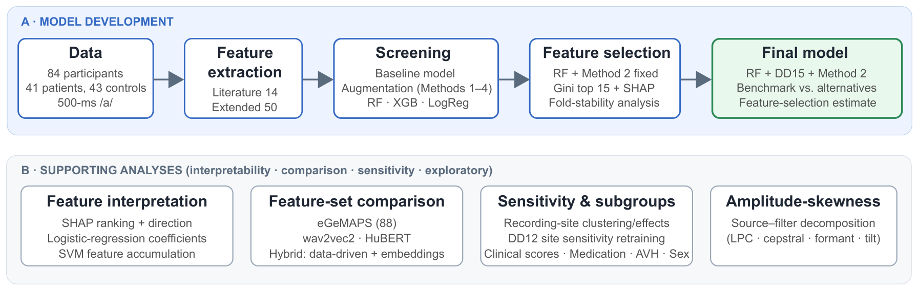
Figure 2.
Representative 500-ms voice segment and five augmented copies generated through conservative perturbations to reflect the natural range of vocal variability. Perturbation types are applied individually here for illustration.
Figure 2.
Representative 500-ms voice segment and five augmented copies generated through conservative perturbations to reflect the natural range of vocal variability. Perturbation types are applied individually here for illustration.
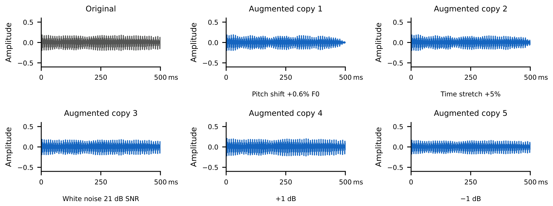
Figure 3.
Baseline classification performance, shown as ROC curves for (a) Literature 14 and (b) Extended 50 feature sets under Method 1 (Original/Original).
Figure 3.
Baseline classification performance, shown as ROC curves for (a) Literature 14 and (b) Extended 50 feature sets under Method 1 (Original/Original).
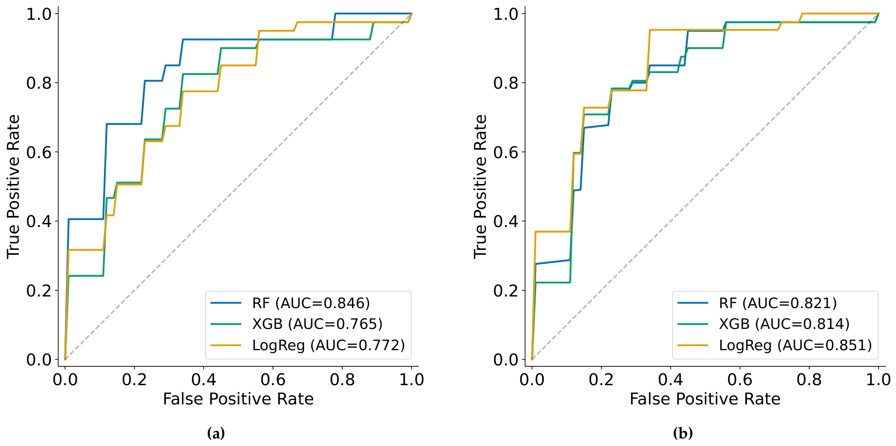
Figure 4.
SHAP feature impact on model output (beeswarm) for the DD15 Random Forest model. Colour encodes feature value (blue low, red high); horizontal position is the SHAP value (impact on patient class prediction).
Figure 4.
SHAP feature impact on model output (beeswarm) for the DD15 Random Forest model. Colour encodes feature value (blue low, red high); horizontal position is the SHAP value (impact on patient class prediction).
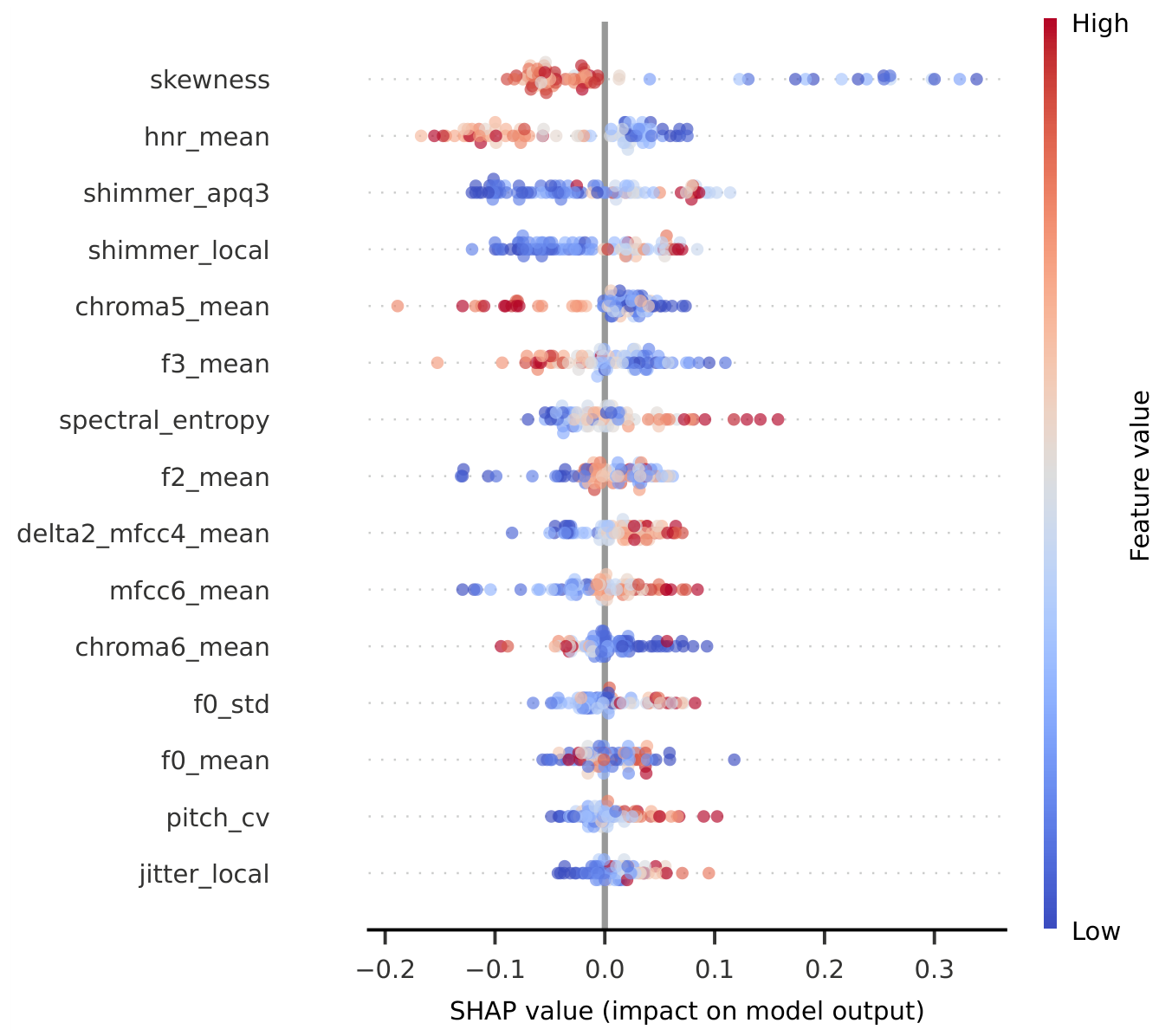
Figure 5.
Confusion matrices of all three classifiers with the Data-driven 15 feature set under Method 2 (Original+Augmented/Original).
Figure 5.
Confusion matrices of all three classifiers with the Data-driven 15 feature set under Method 2 (Original+Augmented/Original).
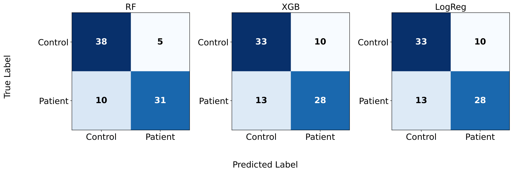
Figure 6.
Final model comparison: (a) ROC curves for all three classifiers with Data-driven 15 feature set under Method 2 (Original+Augmented/Original); (b) Random Forest + DD15 + Method 2 (Original+Augmented/Original) operating points. ROC curve is based on pooled Method 2 (Original+Augmented/Original) predictions; AUC in the legend is the mean cross-validated AUC over 5 folds.
Figure 6.
Final model comparison: (a) ROC curves for all three classifiers with Data-driven 15 feature set under Method 2 (Original+Augmented/Original); (b) Random Forest + DD15 + Method 2 (Original+Augmented/Original) operating points. ROC curve is based on pooled Method 2 (Original+Augmented/Original) predictions; AUC in the legend is the mean cross-validated AUC over 5 folds.
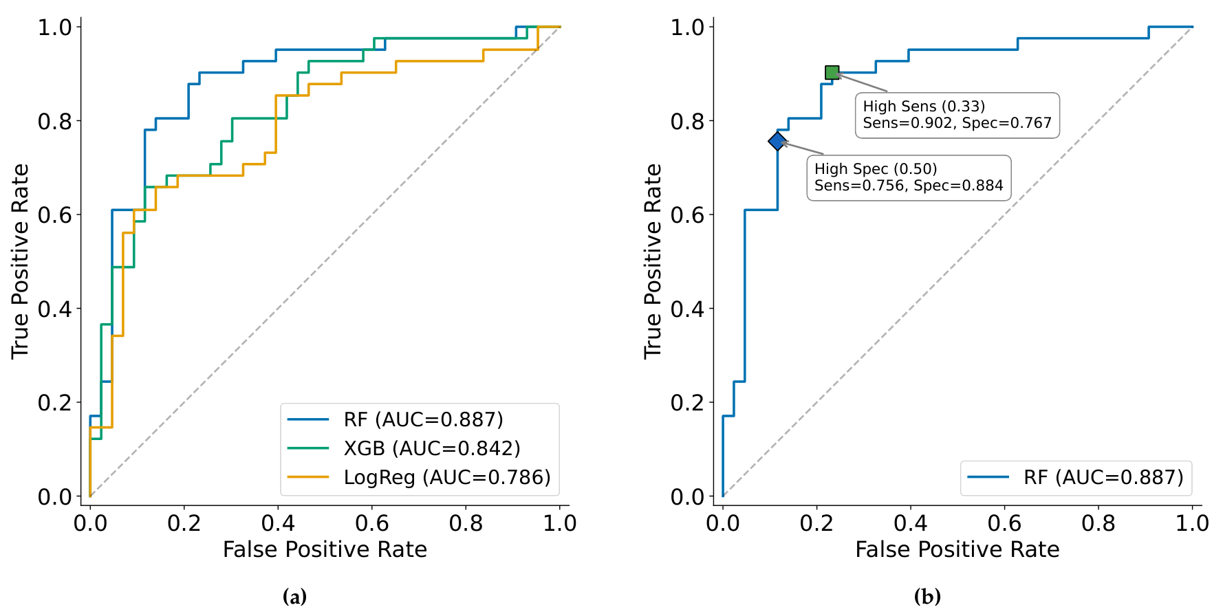
Table 1.
Participant demographics. Mean values with standard deviation are presented where applicable. Between-group p-values are from one-way ANOVA (continuous variables) and Pearson’s chi-square test with Yates’ correction (sex). Chlorpromazine-equivalent dose is reported as CPZ.
Table 1.
Participant demographics. Mean values with standard deviation are presented where applicable. Between-group p-values are from one-way ANOVA (continuous variables) and Pearson’s chi-square test with Yates’ correction (sex). Chlorpromazine-equivalent dose is reported as CPZ.
| Patients () | Controls () | p-value | |
|---|---|---|---|
| Age (years) | 35.12 ± 9.41 | 35.53 ± 9.24 | 0.840 |
| Sex (M/F) | 24/17 | 21/22 | 0.501 |
| PANSS total | 74.20 ± 17.27 | — | — |
| PANSS positive | 15.20 ± 4.82 | — | — |
| PANSS negative | 23.00 ± 6.28 | — | — |
| CPZ equiv. (mg) | 560.41 ± 396.12 | — | — |
| CAPS total | — | 4.65 ± 3.54 | — |
| PDI total | — | 3.95 ± 2.22 | — |
Table 2.
Representative acoustic feature families used in schizophrenia and psychiatric voice research.
Table 2.
Representative acoustic feature families used in schizophrenia and psychiatric voice research.
| Domain | Feature | Description | Repr. use† |
|---|---|---|---|
| Prosodic | F0 mean | Mean fundamental frequency (perceived pitch). | [11,12,16] |
| Prosodic | F0 SD / range | Pitch variability / range; reduced variation linked to aprosody and negative symptoms. | [12,29] |
| Voice quality | Jitter (local) | Cycle-to-cycle frequency perturbation; perceived hoarseness. | [12,16,30] |
| Voice quality | Shimmer (local) | Cycle-to-cycle amplitude perturbation; perceived roughness. | [12,16,30] |
| Voice quality | HNR | Harmonic-to-noise ratio; periodic vs. aperiodic energy. | [12,29,30] |
| Voice quality | CPP / CPPS | Cepstral peak prominence; robust overall dysphonia measure. | [31] |
| Formant | F1–F5 means | Vocal-tract resonance frequencies; vowel quality and timbre. | [16,29] |
| Formant | Formant bandwidths | Resonance bandwidths; vocal-tract damping. | [19] |
| Cepstral | MFCC1–n / delta-MFCCs | Spectral-envelope shape and its temporal dynamics. | [12,16,29] |
| Spectral | Spectral centroid / entropy | Spectral centre of mass; spectral flatness / disorder. | [14,16] |
| Spectral | Spectral tilt / H1–H2 | Spectral slope; glottal-source correlate. | [14] |
| Intensity | Intensity / loudness | Vocal energy; reduced vocal intensity in negative symptoms. | [16] |
†Repr. use = representative examples of use in schizophrenia-spectrum speech/voice research.
Table 3.
Overview of methods with train–test configurations used for data augmentation analyses.
| Method | Training set | Test set | Purpose |
|---|---|---|---|
| Method 1 | Original data | Original data | Baseline classification performance using only original voice recordings. |
| Method 2 | Original data + augmented data | Original data | Evaluates whether adding augmented recordings to the training set improves performance on original recordings. |
| Method 3 | Augmented data | Augmented data | Assesses whether training and testing on augmented recordings artificially inflates classification performance. |
| Method 4 | Augmented data | Original data | Assesses whether a model trained exclusively on augmented recordings generalizes to original recordings. |
Table 4.
Feature representations compared with DD15 under Random Forest, Method 2 (Original+Augmented/Original).
Table 4.
Feature representations compared with DD15 under Random Forest, Method 2 (Original+Augmented/Original).
| Family | Description |
|---|---|
| Handcrafted (study-specific) | Literature 14: literature-derived 14-feature set used in prior schizophrenia voice research; Extended 50: full 50-feature candidate pool defined for the present study. |
| Standardized general-purpose | eGeMAPS: extended Geneva Minimalistic Acoustic Parameter Set, comprising 88 handcrafted temporal, spectral, and energy features and widely used as an interpretable baseline in clinical and affective voice research [18]. |
| Deep learning–based | wav2vec2-base and HuBERT-base: frozen embeddings from self-supervised speech models pretrained on large speech corpora. Hybrid representations combined DD15 with each embedding set [36,37]. |
Table 5.
Baseline classification performance on Literature 14 and Extended 50 feature sets under Method 1 (Original/Original). AUC is reported as mean±SD; all other metrics are mean. Bold indicates the best value per metric.
Table 5.
Baseline classification performance on Literature 14 and Extended 50 feature sets under Method 1 (Original/Original). AUC is reported as mean±SD; all other metrics are mean. Bold indicates the best value per metric.
| Model | Feature Set | AUC | Acc. | Sens. | Spec. | F1 score |
|---|---|---|---|---|---|---|
| Logistic Regression | Literature 14 | 0.772±0.111 | 0.668 | 0.631 | 0.698 | 0.643 |
| Random Forest | Literature 14 | 0.846±0.120 | 0.799 | 0.875 | 0.721 | 0.809 |
| XGBoost | Literature 14 | 0.765±0.099 | 0.715 | 0.706 | 0.721 | 0.707 |
| Logistic Regression | Extended 50 | 0.851±0.049 | 0.762 | 0.731 | 0.794 | 0.748 |
| Random Forest | Extended 50 | 0.821±0.120 | 0.810 | 0.853 | 0.765 | 0.812 |
| XGBoost | Extended 50 | 0.814±0.099 | 0.762 | 0.731 | 0.787 | 0.751 |
Table 6.
Classification performance (AUC) across data augmentation configurations. Values are reported as mean±SD. Bold indicates the best result per model.
Table 6.
Classification performance (AUC) across data augmentation configurations. Values are reported as mean±SD. Bold indicates the best result per model.
| Method | Random Forest | XGBoost | Log. Reg. |
|---|---|---|---|
| Method 1 (Original/Original) | 0.821 ± 0.120 | 0.814 ± 0.099 | 0.851 ± 0.049 |
| Method 2 (Original+Augmented/Original) | 0.842 ± 0.102 | 0.806 ± 0.089 | 0.810 ± 0.081 |
| Method 3 (Augmented/Augmented) | 0.823 ± 0.090 | 0.776 ± 0.073 | 0.790 ± 0.098 |
| Method 4 (Augmented/Original) | 0.826 ± 0.083 | 0.826 ± 0.071 | 0.796 ± 0.122 |
Table 7.
Top 15 features selected by Random Forest Gini importance under Method 2 (Original+Augmented/Original). Importance is the mean Random Forest Gini impurity decrease across the five cross-validation folds. Stability describes selection frequency across folds. Values are on the native Gini scale and sum to 1 across all Extended 50 features.
Table 7.
Top 15 features selected by Random Forest Gini importance under Method 2 (Original+Augmented/Original). Importance is the mean Random Forest Gini impurity decrease across the five cross-validation folds. Stability describes selection frequency across folds. Values are on the native Gini scale and sum to 1 across all Extended 50 features.
| Rank | Feature | Importance | Stability (folds) | Domain |
|---|---|---|---|---|
| 1 | amplitude skewness | 0.0766 | Core (5/5) | Distributional |
| 2 | hnr_mean | 0.0475* | Core (5/5) | Voice quality |
| 3 | shimmer_local | 0.0475* | Core (5/5) | Voice quality |
| 4 | shimmer_apq3 | 0.0450 | Core (5/5) | Voice quality |
| 5 | chroma5_mean | 0.0412 | Core (5/5) | Chroma |
| 6 | spectral_entropy | 0.0390 | Core (5/5) | Spectral |
| 7 | f3_mean | 0.0321 | Near-core (4/5) | Formant |
| 8 | delta2_mfcc4_mean | 0.0316 | Variable (3/5) | Cepstral |
| 9 | chroma6_mean | 0.0290 | Variable (3/5) | Chroma |
| 10 | f0_std | 0.0286 | Near-core (4/5) | Prosodic |
| 11 | f0_mean | 0.0281 | Core (5/5) | Prosodic |
| 12 | f2_mean | 0.0276 | Variable (3/5) | Formant |
| 13 | mfcc6_mean | 0.0265 | Near-core (4/5) | Cepstral |
| 14 | jitter_local | 0.0247 | Unstable (2/5) | Voice quality |
| 15 | pitch_cv | 0.0246 | Unstable (2/5) | Prosodic |
* HNR and local shimmer received near-identical mean Gini importance (unrounded 0.04752 and 0.04749); the 2nd/3rd ordering should be regarded as effectively tied.
Table 8.
Agreement between Gini importance and SHAP rankings for the DD15 features (including SHAP magnitude and direction).
Table 8.
Agreement between Gini importance and SHAP rankings for the DD15 features (including SHAP magnitude and direction).
| Feature | Gini rank | SHAP rank | rank | Mean |SHAP| | Direction (SHAP) |
|---|---|---|---|---|---|
| amplitude skewness | 1 | 1 | = | 0.0813 | Lower → patient |
| hnr_mean | 2 | 2 | = | 0.0620 | Lower → patient |
| shimmer_local | 3 | 4 | 0.0489 | Higher → patient | |
| shimmer_apq3 | 4 | 3 | 0.0597 | Higher → patient | |
| chroma5_mean | 5 | 5 | = | 0.0369 | Lower → patient |
| spectral_entropy | 6 | 7 | 0.0329 | Higher → patient | |
| f3_mean | 7 | 6 | 0.0349 | Lower → patient | |
| delta2_mfcc4_mean | 8 | 9 | 0.0289 | Higher → patient | |
| chroma6_mean | 9 | 11 | 0.0239 | Lower → patient | |
| f0_std | 10 | 12 | 0.0230 | Higher → patient | |
| f0_mean | 11 | 13 | 0.0218 | Lower → patient | |
| f2_mean | 12 | 8 | 0.0303 | Higher → patient | |
| mfcc6_mean | 13 | 10 | 0.0288 | Higher → patient | |
| jitter_local | 14 | 15 | 0.0202 | Higher → patient | |
| pitch_cv | 15 | 14 | 0.0207 | Higher → patient |
Table 9.
DD15 classification results across four training methods and three classifiers. AUC is reported as mean±SD; all other metrics are mean. Bold indicates the best value per metric.
Table 9.
DD15 classification results across four training methods and three classifiers. AUC is reported as mean±SD; all other metrics are mean. Bold indicates the best value per metric.
| Method | Model | AUC | Acc. | Sens. | Spec. | F1 score |
|---|---|---|---|---|---|---|
| Method 1 | Random Forest | 0.873±0.109 | 0.786 | 0.828 | 0.743 | 0.791 |
| Method 1 | XGBoost | 0.796±0.058 | 0.773 | 0.756 | 0.781 | 0.765 |
| Method 1 | Logistic Regression | 0.823±0.142 | 0.737 | 0.686 | 0.787 | 0.718 |
| Method 2 | Random Forest | 0.887±0.078 | 0.823 | 0.753 | 0.889 | 0.799 |
| Method 2 | XGBoost | 0.842±0.078 | 0.725 | 0.686 | 0.765 | 0.704 |
| Method 2 | Logistic Regression | 0.786±0.144 | 0.725 | 0.683 | 0.759 | 0.708 |
| Method 3 | Random Forest | 0.851±0.067 | 0.747 | 0.713 | 0.776 | 0.732 |
| Method 3 | XGBoost | 0.792±0.086 | 0.684 | 0.652 | 0.715 | 0.662 |
| Method 3 | Logistic Regression | 0.788±0.142 | 0.711 | 0.700 | 0.718 | 0.706 |
| Method 4 | Random Forest | 0.886±0.085 | 0.786 | 0.706 | 0.860 | 0.759 |
| Method 4 | XGBoost | 0.824±0.092 | 0.737 | 0.639 | 0.838 | 0.697 |
| Method 4 | Logistic Regression | 0.780±0.148 | 0.738 | 0.658 | 0.810 | 0.709 |
Table 10.
Cross-validation performance with fold-wise feature selection by feature count. AUC with fold-wise selection is reported as mean±SD across folds. Bold indicates the highest mean.
Table 10.
Cross-validation performance with fold-wise feature selection by feature count. AUC with fold-wise selection is reported as mean±SD across folds. Bold indicates the highest mean.
| features | AUC with fold-wise selection |
|---|---|
| 8 | 0.813±0.112 |
| 10 | 0.829±0.123 |
| 12 | 0.858±0.096 |
| 15 | 0.837±0.086 |
Table 11.
Feature set comparison under Random Forest, Method 2 (Original+Augmented/Original) (DD15 vs. Literature 14, Extended 50, eGeMAPS). Bold: best values per metric.
Table 11.
Feature set comparison under Random Forest, Method 2 (Original+Augmented/Original) (DD15 vs. Literature 14, Extended 50, eGeMAPS). Bold: best values per metric.
| Feature Set | AUC | Acc. | Sens. | Spec. | F1 score | |
|---|---|---|---|---|---|---|
| Data-driven 15 | 15 | 0.887±0.078 | 0.823 | 0.753 | 0.889 | 0.799 |
| Literature 14 | 14 | 0.768±0.101 | 0.668 | 0.536 | 0.800 | 0.597 |
| Extended 50 | 50 | 0.842±0.102 | 0.775 | 0.678 | 0.860 | 0.737 |
| eGeMAPS | 88 | 0.861±0.093 | 0.726 | 0.658 | 0.787 | 0.694 |
Table 12.
Pretrained embedding results compared with the final model configuration (all under Method 2, Original+Augmented/Original). AUC is reported as mean±SD. Bold indicates the best value per metric.
Table 12.
Pretrained embedding results compared with the final model configuration (all under Method 2, Original+Augmented/Original). AUC is reported as mean±SD. Bold indicates the best value per metric.
| Configuration | AUC |
|---|---|
| DD15+RF | 0.887±0.078 |
| wav2vec2 last+LR | 0.681±0.102 |
| wav2vec2 inter+RF | 0.745±0.083 |
| HuBERT inter+RF | 0.833±0.137 |
| Hybrid DD15+wav2vec2 RF | 0.862±0.103 |
| Hybrid DD15+HuBERT RF | 0.862±0.104 |
Table 13.
Comparison of DD15 feature importance ranks across Random Forest Gini, SHAP, and logistic regression. The direction comparison is between SHAP and logistic regression. Ranks agree closely between the two tree-based methods and diverge from the linear model (Spearman = 0.143, p = 0.61).
Table 13.
Comparison of DD15 feature importance ranks across Random Forest Gini, SHAP, and logistic regression. The direction comparison is between SHAP and logistic regression. Ranks agree closely between the two tree-based methods and diverge from the linear model (Spearman = 0.143, p = 0.61).
| Feature | Gini | SHAP | Log. Reg. | Direction |
|---|---|---|---|---|
| amplitude skewness | 1 | 1 | 1 | Lower → patient |
| hnr_mean | 2 | 2 | 5 | Lower → patient |
| shimmer_local | 3 | 4 | 12 | Higher → patient |
| shimmer_apq3 | 4 | 3 | 15 | Higher → patient |
| chroma5_mean | 5 | 5 | 7 | Lower → patient |
| spectral_entropy | 6 | 7 | 13 | Mixed* |
| f3_mean | 7 | 6 | 2 | Lower → patient |
| delta2_mfcc4_mean | 8 | 9 | 4 | Higher → patient |
| chroma6_mean | 9 | 11 | 10 | Lower → patient |
| f0_std | 10 | 12 | 9 | Higher → patient |
| f0_mean | 11 | 13 | 14 | Lower → patient |
| f2_mean | 12 | 8 | 11 | Higher → patient |
| mfcc6_mean | 13 | 10 | 3 | Higher → patient |
| jitter_local | 14 | 15 | 8 | Higher → patient |
| pitch_cv | 15 | 14 | 6 | Higher → patient |
* Mixed: SHAP higher→patient, logistic regression higher→control
Table 14.
Diagnostic effect sizes and recording site effects for DD15 features. Cohen’s d was computed as patients minus controls. Site and the Kruskal–Wallis p-value describe variation among the seven control sites. The final column indicates whether the mean feature value across all patients lay outside the minimum-to-maximum range of the seven site-specific control means.
Table 14.
Diagnostic effect sizes and recording site effects for DD15 features. Cohen’s d was computed as patients minus controls. Site and the Kruskal–Wallis p-value describe variation among the seven control sites. The final column indicates whether the mean feature value across all patients lay outside the minimum-to-maximum range of the seven site-specific control means.
| Feature | Cohen’s | Site | Site (KW) | Patient group mean outside control site mean range |
|---|---|---|---|---|
| amplitude skewness | 0.095 | 0.777 | Yes | |
| hnr_mean | 0.181 | 0.611 | Yes | |
| shimmer_local | 0.254 | 0.214 | Yes | |
| shimmer_apq3 | 0.250 | 0.227 | No | |
| chroma5_mean | 0.058 | 0.793 | Yes | |
| spectral_entropy | 0.079 | 0.735 | No | |
| f3_mean | 0.119 | 0.725 | No | |
| delta2_mfcc4_mean | 0.172 | 0.243 | No | |
| chroma6_mean | 0.160 | 0.300 | No | |
| f0_std | 0.105 | 0.313 | Yes | |
| f0_mean | 0.345 | 0.027 | No | |
| f2_mean | 0.248 | 0.133 | No | |
| mfcc6_mean | 0.292 | 0.029 | No | |
| jitter_local | 0.127 | 0.459 | Yes | |
| pitch_cv | 0.026 | 0.994 | Yes |
Table 16.
Sex-stratified performance under Random Forest + DD15 + Method 2 (Original+Augmented/Original). AUC is reported as mean±SD. Bold indicates the best value per metric.
Table 16.
Sex-stratified performance under Random Forest + DD15 + Method 2 (Original+Augmented/Original). AUC is reported as mean±SD. Bold indicates the best value per metric.
| Group | AUC | Acc. | Sens. | Spec. | F1 score |
|---|---|---|---|---|---|
| Overall | 0.823 | 0.753 | 0.889 | 0.799 | |
| Males | 0.711 | 0.703 | 0.683 | 0.710 | |
| Females | 0.871 | 0.720 | 1.000 | 0.817 |
Disclaimer/Publisher’s Note: The statements, opinions and data contained in all publications are solely those of the individual author(s) and contributor(s) and not of MDPI and/or the editor(s). MDPI and/or the editor(s) disclaim responsibility for any injury to people or property resulting from any ideas, methods, instructions or products referred to in the content. |
© 2026 by the authors. Licensee MDPI, Basel, Switzerland. This article is an open access article distributed under the terms and conditions of the Creative Commons Attribution (CC BY) license (http://creativecommons.org/licenses/by/4.0/).
Copyright: This open access article is published under a Creative Commons CC BY 4.0 license, which permit the free download, distribution, and reuse, provided that the author and preprint are cited in any reuse.