

Submitted:
30 August 2026
Posted:
31 August 2026
You are already at the latest version
Abstract
Residential microgrids are expected to enhance both environmental sustainability and disaster resilience in future housing developments. This study investigates two distributed control schemes for residential DC microgrids: an autonomous distributed cooperative control based on the state of charge (SoC) of battery-driven DC/DC converters, and an autonomous decentralized control based solely on feeder voltage, enabled by directly connected distributed batteries. A detailed DC microgrid model consisting of five houses was constructed in MATLAB/Simulink, incorporating PV panels with different orientations, small wind turbines, household load profiles, EV charging, and realistic meteorological data. The cooperative control scheme effectively stabilized feeder voltage, suppressed surplus renewable generation, and reduced reverse power flow to the utility grid. The decentralized scheme also maintained stable feeder voltage without device-to-device communication, although it resulted in greater reverse power flow due to less effective generation curtailment. In both schemes, houses near the grid-interconnection point experienced more frequent battery cycling, indicating the need for larger battery capacities at those locations. Simulations showed that installing approximately 20 kWh of battery capacity per house enables more than 80% of annual consumption can be obtained from renewable energy and allows continued operation during off-grid conditions with reduced consumption. These results demonstrate the practical feasibility of distributed-control residential microgrids.
Keywords:
DC microgrid
; residential microgrid
; MATLAB/Simulink
; simulation
; renewable energy
; photovoltaic generation
; wind power
; autonomous decentralized control
; autonomous distributed cooperative control
1. Introduction
Future residential houses equipped with renewable-energy generation systems—such as photovoltaic (PV) panels and wind turbines—together with battery storage are expected to play a key role in promoting environmentally sustainable lifestyles. By enabling local production and consumption of renewable electricity, such houses can reduce dependence on conventional power systems and maintain a certain level of energy autonomy even during disasters, thereby enhancing both environmental performance and resilience. However, if each household attempts to operate independently with its own renewable generation and storage systems, the required installation capacity becomes considerably large [1,2]. This poses practical challenges in terms of installation space and cost, making full self-sufficiency difficult to achieve under current technological and economic conditions.
To address this issue, multiple houses can be interconnected through dedicated power lines to form a residential microgrid. In such a configuration, even if one house experiences a temporary shortage of electricity, surplus energy from other houses can be shared within the microgrid. This cooperative structure reduces the required battery capacity and other equipment sizes for each individual house [3,4,5]. Nevertheless, relying solely on intermittent and unstable renewable generation may still lead to energy shortages at the microgrid level. Therefore, interconnection with the existing utility grid remains essential to ensure stable operation and enable bidirectional power exchange when necessary.
Although numerous studies have discussed residential microgrids [6,7,8,9,10,11,12,13,14,15,16,17,18], relatively few have examined their control strategies and required equipment capacities in a concrete and quantitative manner. In this study, we investigate practical control methods for residential microgrids through detailed simulations using MATLAB/Simulink. Particular emphasis is placed on decentralized control, and two representative decentralized control schemes are compared through simulation-based analysis. The key aspects examined include the stability of feeder voltage across the entire microgrid, the magnitude of power exchange with the utility grid, the required battery capacity, and the expected battery lifetime.
To conduct this analysis, we extended our previously developed microgrid simulator by incorporating additional device models, including battery-driven power converters and wind turbines. The PV model was also enhanced to account for panel orientation. The structure of this paper is as follows. Section 2 describes the general configuration of residential microgrids and defines the specific system considered in this study. Section 3 explains the control strategies for residential microgrids, with particular focus on the two decentralized control schemes compared in this work. Section 4 presents simulation results obtained using the microgrid simulator and compares the operational characteristics of the two control approaches. Section 5 discusses the required battery capacity for optimal system design and examines off-grid operation scenarios, such as during disasters. Finally, Section 6 concludes the paper.
2. Configuration of Residential Microgrids
Residential microgrids can be broadly categorized into two types: AC microgrids, in which the main feeder is constructed using alternating current, and DC microgrids, in which the feeder is based on direct current. In AC microgrids, the system is normally interconnected with the utility grid and operates in a grid-synchronized mode. Energy balancing within the microgrid relies heavily on the utility grid, and the electrical inertia required to accommodate sudden and large load fluctuations is also provided by the grid. However, during disasters or other events that cause the utility grid to shut down, the microgrid must disconnect from the grid and operate independently. In such islanded operation, the microgrid must form its own AC grid and provide the necessary inertia and stability. Therefore, AC microgrids require dedicated grid-forming units—typically engine-driven generators—that remain on standby during normal operation but must be capable of immediate activation when the system transitions to off-grid mode [19,20].
In contrast, DC microgrids employ multiple battery-driven DC/DC converter units connected in parallel as voltage sources on the main feeder, enabling the microgrid to form and maintain its own DC grid regardless of whether it is operating under grid-connected or off-grid conditions. The electrical inertia required to respond to sudden load variations must also be provided internally within the microgrid. When the microgrid is connected to the utility grid and capable of bidirectional power exchange (on-grid mode), the grid can supplement energy balancing during normal conditions. However, during disasters when the utility grid is unavailable, this support cannot be relied upon. Consequently, DC microgrids must be equipped with sufficiently large battery storage to manage energy balancing autonomously.
Silicon-based PV panels have become widely adopted as residential renewable-energy generators due to their affordability and long service life, typically exceeding 20 years. Small-scale wind turbines have also become increasingly common in residential areas. Although battery systems remain relatively expensive compared with PV and wind turbines, the cost of lithium iron phosphate (LiFePO₄) batteries has significantly decreased over the past decade due to large-scale production in China. Renewable-energy generators such as PV panels and wind turbines, as well as battery storage systems, can be integrated into both AC and DC microgrids. However, DC microgrids generally require fewer power-conversion stages to interface these devices with the main feeder, resulting in lower conversion losses [21,22,23]. Furthermore, AC systems require management of not only voltage but also frequency, phase, and reactive power, whereas DC systems require control only of voltage and current (power) [24,25]. From a control perspective, DC microgrids are therefore considerably simpler. For these reasons, this study focuses on residential microgrids based on DC feeders.
Although interconnection with the utility grid is essential for residential microgrids that rely primarily on intermittent renewable generation, the dependence on the grid should be minimized. Power exchange with the utility grid should occur only when necessary and should be limited in magnitude and duration. The microgrid is assumed to have a single point of interconnection with the utility grid. In Japan, distribution networks typically operate at 6.6 kV, but such high voltages are unsuitable for residential microgrids due to safety considerations. Therefore, the feeder voltage must be kept relatively low, typically on the order of a few hundred volts [26,27]. In this study, a commonly used DC feeder voltage of 380 V is adopted. Even when relatively thick cables (e.g., 8-SQ copper conductors) are used, conductor resistance cannot be neglected. As shown later in the analysis, power flow along the feeder causes voltage differences of several volts depending on location. This leads to spatial imbalance in energy distribution within the microgrid, necessitating mechanisms to equalize energy among different nodes.
3. Control of Residential DC Microgrids
3.1. Distributed Control Schemes
In conventional utility power systems, power flow and energy balancing across the entire grid are centrally monitored and controlled by the utility operator’s dispatch center. In contrast, distributed control is more suitable for small-scale residential microgrids [28]. Installing a central controller for each residential microgrid is impractical due to operational costs. Moreover, in residential areas where houses are frequently renovated or expanded, each modification would require rewiring communication links to the central controller and updating control algorithms. Without a plug-and-play mechanism, such a system would be unacceptable for residential users. Additionally, if the central controller fails or its communication lines are damaged during a disaster, the entire microgrid would become uncontrollable [29]. For these reasons, a decentralized and democratic control approach—one in which residents can participate in operation and respond to faults or modifications—is desirable for residential microgrids.
Distributed control can be broadly classified into two categories [30,31,32,33]. The first is autonomous distributed cooperative control, in which neighboring devices communicate, exchange power-related information, negotiate operational decisions, and coordinate their actions to achieve partial optimization. The second is autonomous decentralized control, in which no communication occurs among devices; each device operates independently based solely on its own local measurements and decision-making.
An example of autonomous distributed cooperative control is a scheme in which the operation of generation and load devices is coordinated based on the state of charge (SoC) of nearby distributed batteries. In this case, the controllers of PV panels, wind turbines, and loads must be connected to distributed batteries via communication lines to receive SoC information. Figure 1 illustrates the conceptual configuration of autonomous distributed cooperative control.
In autonomous decentralized control, no information exchange, negotiation, or coordination occurs among devices. Each device must determine its own operation based solely on locally collected information. The decision criteria are: (1) whether the device can fulfill its intended function, and (2) whether its operation would adversely affect the microgrid. For example, a power-load device aims to operate when needed, and a power-generation device aims to supply as much power as possible to the feeder. However, such operation must not destabilize the microgrid. Therefore, each device senses feeder voltage and current to determine whether it is appropriate to begin operation. This approach assumes that feeder voltage and current reflect the health of the microgrid. Figure 2 shows the conceptual configuration of autonomous decentralized control.
3.2. Residential Microgrid Control Based on Autonomous Distributed Cooperative Control
In this scheme, each house is equipped with a battery-driven DC/DC converter connected to the DC feeder. When the battery’s SoC is within the normal operating range, the DC/DC converter supplies power to the feeder or draws power from it to charge the battery, thereby functioning as a grid-forming voltage source that maintains the feeder voltage at a prescribed level. Furthermore, each house’s power system transmits battery SoC information to the PV controller. When the battery approaches full charge and no longer has capacity to absorb surplus PV generation, the PV controller reduces or stops generation accordingly.
For houses connected to the utility grid, the power-exchange unit also communicates with the battery system. When the battery SoC falls below the normal range, power is imported from the utility grid; conversely, when the SoC exceeds the normal range, surplus energy is exported to the grid. Household appliances, however, do not communicate with other devices. They operate freely according to user demand, provided that the feeder voltage remains within the allowable range for safe operation.
3.3. Residential Microgrid Control Based on Autonomous Decentralized Control
In this scheme, no communication occurs among devices. Each device must assess the microgrid’s condition and determine its own operation independently. The only information available to devices connected to the feeder is feeder voltage and current. Therefore, a mechanism is required to ensure that feeder voltage reflects the operational state of the microgrid.
We previously proposed the concept of a battery-integrated feeder [34,35], in which distributed batteries—such as lithium-ion batteries whose terminal voltage varies nearly linearly with SoC—are directly connected to the feeder with equalized terminal voltages. In such a configuration, the feeder voltage reflects the SoC of nearby batteries. By measuring feeder voltage, devices can infer the local battery SoC.
Devices connected to the feeder then determine power exchange based solely on feeder voltage. For example, a load device interprets high feeder voltage as an indication of sufficient nearby battery capacity and begins operation. If feeder voltage is low, it refrains from operating. Similarly, a generation device interprets moderately low feeder voltage as an indication of available battery capacity and injects power into the feeder. If feeder voltage is high, it interprets this as the battery approaching full charge and stops generation. With such a mechanism, devices can operate autonomously without communication while maintaining microgrid stability.
4. Analysis of the Residential DC Microgrid
4.1. MATLAB/Simulink Model of the Residential DC Microgrid
To analyze the distributed control behavior described in the previous section, simulation-based evaluation was conducted using MATLAB/Simulink. In our earlier work, we developed a DC-grid simulator capable of analyzing autonomous decentralized control based on the battery-integrated feeder concept [8]. In the present study, the simulator was extended to incorporate additional device models, including battery-driven voltage sources and wind turbines, enabling analysis of autonomous distributed cooperative control. The PV model was also enhanced to account for panel installation orientation. Using the extended simulator, a residential DC microgrid consisting of five houses was constructed.
Figure 3 illustrates the conceptual configuration of the modeled residential microgrid. Each house is equipped with rooftop PV panels rated at 3.5 kW, corresponding to the typical installation capacity for a standard detached house in Japan. To reflect realistic installation conditions, the orientation of the PV panels differs among houses, resulting in distinct temporal variations in incident solar irradiance and, consequently, different generation profiles even with identical rated capacities. Details of the PV device model are provided in Appendix A.1.
All houses are interconnected by a DC feeder with a nominal voltage of 380 V. The distance between houses was assumed to be 30 m—slightly larger than the typical spacing of 10–15 m in Japanese residential areas—and the feeder cable length between houses was set accordingly. An 8-SQ copper conductor was used for the feeder cable, providing an allowable current exceeding 60 A, which is more than sufficient given that actual feeder currents remain below 15 A, as shown in Section 4.2.
Daily electricity consumption for each house was generated using random variations to reflect household-specific differences, while monthly consumption followed statistical data. Hourly consumption patterns were based on typical residential load profiles. Details of the residential load model are provided in Appendix A.3. House 3, located at the center of the microgrid, includes an EV charger that operates daily from 2:00 to 4:00 AM, drawing 5 kW for EV charging.
Two small wind turbines were also installed within the residential area and connected to the microgrid at two locations. Given the practical constraints of residential installations, each turbine was rated at 500 W, providing a combined capacity of 1 kW—significantly smaller than the PV capacity of each house and therefore serving only as supplemental generation. Details of the wind turbine model are provided in Appendix A.2.
4.2. Autonomous Distributed Cooperative Control Model
In the autonomous distributed cooperative control model, each house is equipped with a battery-driven DC/DC converter connected to the DC feeder. As detailed in Appendix A.4, the converter model consists of a DC voltage source connected in series with a large capacitor representing the battery. Each house is assumed to have a battery capacity of 10 kWh. When the battery SoC is within the range of 5%–95%, the DC/DC converter operates as a grid-forming voltage source, maintaining the feeder voltage at 380 V. When the battery SoC decreases to 5%, the converter stops discharging to prevent over-discharge and enters a charge-only mode. Once the SoC recovers to 10%, the converter resumes both charging and discharging. Conversely, when the SoC increases to 95%, the converter stops charging to prevent overcharging and enters a discharge-only mode. It resumes normal operation when the SoC decreases to 90%. To prioritize feeder voltage regulation, charging is permitted only when the feeder voltage exceeds 380 V, and discharging is permitted only when the feeder voltage falls below 380 V.
PV and wind turbine controllers are assumed to be connected to the nearest house’s battery system via local communication lines. When the battery SoC reaches 95%, generation is curtailed; when the SoC falls to 90%, generation resumes. House 3 is connected to the utility distribution grid, and its battery system communicates with the grid power-exchange unit. When the battery SoC falls to 10%, the microgrid imports power from the utility grid at a constant current of 25 A until the SoC reaches 15%. Conversely, when the SoC rises to 90%, the microgrid exports power to the grid at 25 A until the SoC decreases to 85%. Details of the power-exchange device model are provided in Appendix A.6.
Table 1 summarizes the specifications of the autonomous distributed cooperative control microgrid model. Figure 4 shows the simulation interface for the residential microgrid under this control scheme.
Meteorological data for Sendai City, Japan, in 2023—consisting of hourly solar irradiance, ambient temperature, and wind speed—were used for the simulations. These data were obtained from the Japan Meteorological Agency website [36]. The hourly data were interpolated with smoothing to generate 1-second interval datasets, which were then used for simulations with a 1-second time step. All converted 1-second MATLAB datasets used in this study have been published in our Zenodo repository [37]. After loading the required data into the MATLAB workspace, the simulation begins and various graphs are displayed on multiple Scope blocks. A full-year simulation completes within a few minutes.
Figure 5 summarizes the annual voltage profiles at various points in the microgrid. Graph (a) shows the feeder voltage at the grid-interconnection point, while graphs (b)–(f) show voltages at the connection points of each house. Although the nominal feeder voltage is 380 V, all measured voltages remain within the range of 365–390 V, demonstrating that the feeder voltage is regulated within ±3% throughout the year.
Figure 6 summarizes the annual PV generation profiles. Graph (a) shows the output of House 1’s east-facing panel installed at a 30° tilt. Graph (b) overlays the outputs of House 2 and House 4, both equipped with south-facing panels at 30°. Graph (c) shows the output of House 3’s zenith-facing panel, and graph (d) shows the output of House 5’s west-facing panel. As expected, the south-facing panels of Houses 2 and 4 produce the highest annual energy, but the zenith-facing and west-facing panels also achieve relatively high generation. House 1’s east-facing panel exhibits lower output, particularly in winter, reflecting Sendai’s typical weather pattern of cloudy mornings and clearer afternoons. Because the PV model accounts for panel temperature, the simulation also reproduces the tendency for summer generation (June–August) to be lower than spring generation (March–April) due to higher panel temperatures. Graphs (e) and (f) show weekly generation profiles for January 1–7 and June 1–7, respectively. In graph (e), south- and west-facing panels maintain relatively high output even in winter. In graph (f), June 2 shows almost no generation due to continuous rainfall, while other days exhibit frequent curtailment events that reduce output to zero.
Figure 7 shows the annual wind-power generation profiles. Periods during which the turbines reach their rated output of 500 W are rare, indicating that wind power contributes far less than PV generation in Sendai. Thus, wind turbines serve only as supplemental sources in residential applications.
Figure 8(a)–(e) shows the annual electricity consumption of each house. In the simulator, power drawn from the microgrid is represented as negative values, so consumption appears as negative power. The consumption patterns differ among houses. Graph (f) overlays the consumption of all houses and EV charging for the week of January 1–7. The nighttime EV charging load of 5 kW is significantly larger than typical household consumption.
Figure 9 shows the annual current profiles flowing through each segment of the feeder cable: (a) between House 1 and House 2, (b) between House 2 and House 3, (c) between House 3 and House 4, and (d) between House 4 and House 5. Positive current corresponds to flow toward the right in Figure 4. The maximum current is approximately 10 A, well below the 65 A allowable current of the 8-SQ CV cable. Currents tend to be highest near the grid-interconnection point and lower toward the feeder ends.
Figure 10(a)–(e) shows the annual SoC profiles of the battery-driven power sources installed in Houses 1–5. Batt3, the battery in House 3, is referenced by the grid power-exchange unit and is controlled within the expected range of 10%–90%. In contrast, the batteries in the other houses fluctuate between 5% and 95%, frequently reaching empty (5%) or full (95%) and triggering charge/discharge suppression. Although each house is equipped with a 10 kWh battery, a slightly larger capacity would be preferable. Notably, even without explicit SoC equalization among houses, the microgrid remains stable.
Figure 11 shows cumulative household consumption, cumulative power imported from the utility grid, and cumulative power exported to the grid. “Power from grid” represents cumulative imported energy, “Power to grid” represents cumulative exported energy, and “Power consumption” represents total consumption of the five houses including EV charging. The vertical axis is expressed in W·sec; converting to kWh yields annual totals of 24,180 kWh for consumption, 6,372 kWh for imported energy, and 2,471 kWh for exported energy. More than 75% of total consumption is supplied by renewable generation.
Figure 12 shows the annual cumulative charge/discharge current of each battery-driven power source, expressed in A·sec. House 3, located at the feeder center and connected to the utility grid, experiences the highest charge/discharge activity, totaling approximately 20 kAh per year. Considering the cycle life of LiFePO₄ batteries (approximately 3,000 cycles) [38,39,40], the estimated lifetime is about 7.9 years. Therefore, if a lifetime of at least 10 years is desired, the battery capacity of House 3 should be increased.
4.3. Autonomous Decentralized Control
In the autonomous decentralized control model, each house is equipped with a LiFePO₄ battery directly connected to the DC feeder. As a result, the battery SoC is reflected in the feeder voltage, enabling each device to infer the condition of the nearby microgrid—specifically, the SoC of distributed batteries—by measuring feeder voltage. Details of the LiFePO₄ battery model are provided in Appendix A.5.
PV and wind turbine controllers rely solely on the voltage measured at their connection point to the feeder. Specifically, generation is curtailed when the local feeder voltage reaches 400 V (i.e., output to the feeder is stopped, although generation itself may continue internally), and generation resumes when the voltage decreases to 398 V. This simple autonomous control requires no communication with other devices.
House 3, located at the center of the microgrid, is connected to the utility grid and performs power exchange through a grid power-exchange unit. The power-exchange unit also operates without communication and relies solely on the feeder voltage at its connection point. When the feeder voltage drops to 360 V—below the nominal 380 V—the microgrid begins importing power from the utility grid. Import continues until the voltage recovers to 370 V. Conversely, when the feeder voltage rises to 400 V, the microgrid begins exporting power to the grid, and export continues until the voltage decreases to 390 V. The stability of the microgrid under such simple voltage-based control is evaluated through simulation.
Table 2 summarizes the specifications of the autonomous decentralized control microgrid model, and Figure 13 shows the simulation interface. Compared with the autonomous distributed cooperative control model in Figure 4, the battery-driven power sources in each house are replaced with LiFePO₄ batteries.
Figure 14 shows the annual voltage profiles at various points in the microgrid. Graph (a) shows the feeder voltage at the grid-interconnection point, while graphs (b)–(f) show voltages at the connection points of each house. Although the nominal feeder voltage is 380 V, all voltages remain within the range of 360–400 V, demonstrating regulation within ±5%. PV generation, wind-power generation, and household consumption profiles are similar to those observed in the autonomous distributed cooperative control model and are therefore omitted here. Feeder currents also remain within ±15 A, well below the allowable current of the 8-SQ cable.
A notable difference from the cooperative control model appears in Figure 15, which shows cumulative household consumption, cumulative grid import, and cumulative grid export. Total annual consumption for the five houses remains 24,180 kWh. However, annual grid import increases to 7,006 kWh, and annual grid export increases to 7,442 kWh—both higher than in the cooperative control case. In particular, grid export (reverse power flow) increases significantly. This is because generation curtailment based on SoC is more effective in the cooperative control model, whereas voltage-based control allows surplus generation to be exported to the grid. As a result, annual grid export slightly exceeds annual grid import, indicating that total renewable generation surpasses total consumption.
Figure 16 shows the annual cumulative charge/discharge current of each battery. As in the cooperative control model, House 3—located at the feeder center and connected to the utility grid—experiences the highest charge/discharge activity, totaling approximately 18 kAh per year. Considering the cycle life of LiFePO₄ batteries (approximately 3,000 cycles), the estimated lifetime is about 6.6 years. The batteries in other houses exhibit lifetimes of approximately 8.3 years. Therefore, to achieve a lifetime exceeding 10 years, battery capacities should be increased beyond 20 Ah.
5. Considerations on Battery Capacity
Based on the results of the previous section, it is evident that the battery capacity installed in each house should be larger. Therefore, we investigated how grid import and export change with battery capacity. In the autonomous distributed cooperative control simulation of Section 4.2, each house was equipped with a 10 kWh battery. When only battery capacity was varied, grid import and export changed as shown in Table 3. Although total annual consumption remains unchanged, both grid import and grid export decrease as battery capacity increases. Figure 17 plots these results, showing that the reduction saturates around 20 kWh. With a 20 kWh battery, more than 83% of total consumption is supplied by renewable generation.
In the autonomous decentralized control simulation of Section 4.3, each house was equipped with a 20 Ah battery. Considering the feeder voltage of 380 V, this corresponds to approximately 7.6 kWh—slightly smaller than the 10 kWh used in Section 4.2. When battery capacity was varied, grid import and export changed as shown in Table 4. Figure 18 plots these results, again showing saturation around 50 Ah (approximately 20 kWh). With a 50 Ah battery, more than 85% of total consumption is supplied by renewable generation. Thus, in both control schemes, a battery capacity of approximately 20 kWh per house is desirable. Larger battery capacity also proportionally increases battery lifetime, enabling lifetimes well beyond 10 years.
Finally, we examined whether the microgrid can sustain power supply during off-grid operation—such as during disasters—when each house is equipped with a 20 kWh battery. During disasters, electricity usage is expected to decrease; therefore, consumption was reduced to 50% of normal levels, and EV charging was disabled. Under these conditions, the grid power-exchange thresholds were modified to prevent any grid import or export. Figure 19 shows cumulative energy profiles for (a) autonomous distributed cooperative control and (b) autonomous decentralized control. In both cases, no grid exchange occurs, and the microgrid successfully maintains power supply throughout off-grid operation.
The complete residential microgrid model used in this study, along with the detailed user manual for the DC grid simulator, has been made publicly available on GitHub [41].
6. Conclusions
This study examined two distributed control schemes for residential DC microgrids through detailed simulations using MATLAB/Simulink. A microgrid model consisting of five houses interconnected by a 380 V DC feeder was constructed, and the autonomous distributed cooperative control scheme—based on the SoC of battery-driven DC/DC converters—was compared with the autonomous decentralized control scheme, in which distributed batteries are directly connected to the feeder and feeder voltage reflects local SoC conditions.
In the autonomous distributed cooperative control scheme, SoC information from each house’s battery-driven DC/DC converter is transmitted to nearby PV and wind generation controllers and to the grid power-exchange unit. This enables effective generation curtailment when batteries approach full charge and stable regulation of feeder voltage. Surplus renewable generation is also prevented from causing excessive reverse power flow to the utility grid.
In contrast, the autonomous decentralized control scheme requires no communication among devices. Distributed batteries are directly connected to the feeder, allowing feeder voltage to represent local SoC conditions. PV, wind generators, and the grid power-exchange unit operate solely based on feeder voltage. Although feeder voltage can be stabilized under this scheme, surplus renewable generation results in greater reverse power flow compared with the cooperative control scheme.
Both control schemes exhibit a common characteristic: houses located closer to the grid-interconnection point experience more frequent battery charge/discharge cycles. To equalize battery lifetime across the microgrid, larger battery capacities should be installed in houses near the grid-interconnection point.
The influence of battery capacity on grid import and export was also investigated. The results show that equipping each house with a battery capacity of approximately 20 kWh enables more than 80% of total annual consumption to be supplied by renewable generation. Furthermore, with 20 kWh batteries, the microgrid can sustain off-grid operation during disasters, provided that household consumption is reduced to 50% of normal levels and EV charging is suspended.
Overall, the results demonstrate that residential DC microgrids employing distributed control—whether cooperative or decentralized—are technically feasible and highly effective. With PV panels rated at approximately 3.5 kW and battery capacities of around 20 kWh per house, such microgrids can achieve high renewable-energy penetration, maintain stable operation, and provide resilience during grid outages. These findings suggest that distributed-control residential DC microgrids represent a practical pathway toward environmentally sustainable and disaster-resilient urban communities.
Future work will include extending the simulator to larger microgrid configurations, incorporating additional distributed energy resources, and validating the proposed control schemes through hardware-in-the-loop experiments or field demonstrations.
Supplementary Materials
The complete Simulink models, MATLAB scripts, and all associated resources used in this study are openly available on GitHub: https://github.com/hiro1959/dc-microgrid-simulator. The meteorological datasets and additional simulation data (1-second resolution) are archived on Zenodo: https://doi.org/10.5281/zenodo.21720183.
Author Contributions
Conceptualization, H.Y.; Methodology, H.Y; Software, H.Y. and K.L.; Validation, H.Y. and K.L.; Formal analysis, H.Y.; Investigation, H.Y. and K.L.; Resources, H.Y.; Data curation, H.Y. and K.L.; Writing—original draft preparation, H.Y.; Writing—review and editing, H.Y. and K.L.; Visualization, H.Y. and K.L.; Supervision, H.Y.; Project administration, H.Y.; Funding acquisition, H.Y. All authors have read and agreed to the published version of the manuscript.
Funding
This research was funded by the JST OPERA Prog. (Grant Number JPMJOP1852).
Data Availability Statement
All data generated or analyzed in this study are included within the article and its Supplementary Materials. Additional inquiries can be directed to the corresponding author.
Acknowledgments
Through the JST OPERA project, the authors had many valuable discussions with K. Iwatsuki and T. Otsuji. The authors would like to express deep gratitude to them.
Conflicts of Interest
The authors declare no conflicts of interest. The funders had no role in the design of this study; in the collection, analyses, or interpretation of data; in the writing of the manuscript; or in the decision to publish the results.
Abbreviations
The following abbreviations are used in this manuscript:
| AC | Alternating current |
| CV cable | Cross-linked polyethylene insulated Vinyl sheath cable |
| DC | Direct current |
| EV | Electric Vehicle |
| LiFePO4 | lithium iron phosphate |
| PV | Photovoltaic |
| SoC | State of charge |
| SQ | square millimeters (mm2) |
Appendix A. Device Models
This appendix summarizes the MATLAB/Simulink device models used in the simulations presented in this study.
Appendix A.1. Photovoltaic Generation
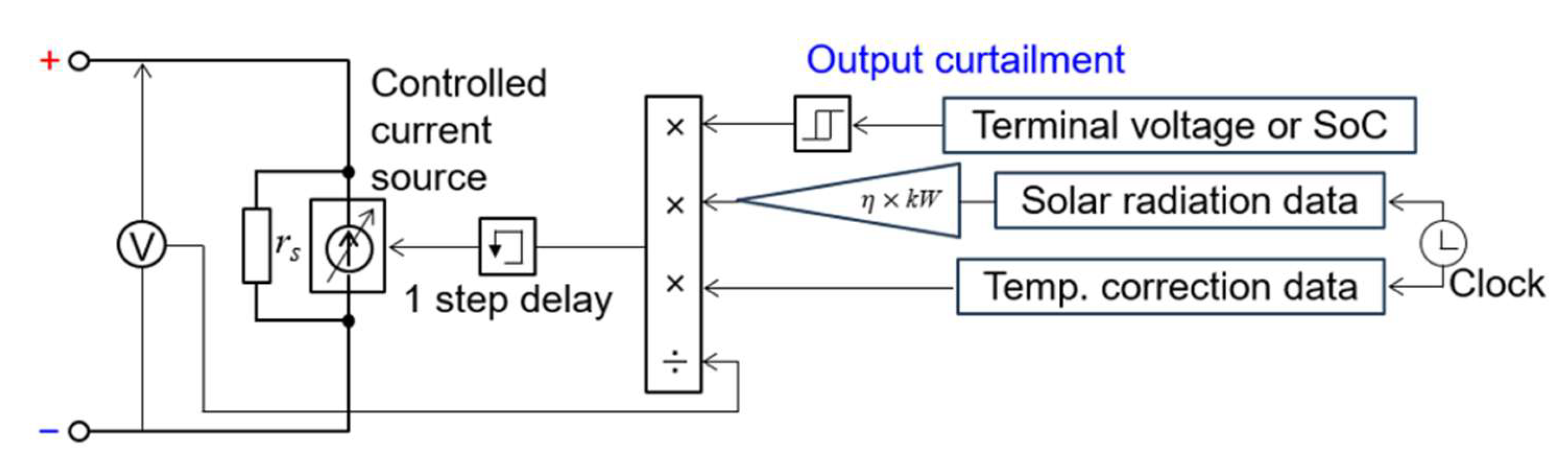
Figure A1 illustrates the conceptual PV device model. The PV output power is calculated by multiplying the plane-of-array (POA) irradiance—precomputed for each panel orientation—by the panel’s rated capacity (kW) and installation efficiency η, followed by a temperature-dependent correction factor. This value is then multiplied by a curtailment flag (normally 1, and 0 when curtailment is required based on battery SoC). The resulting power is divided by the device terminal voltage and fed into the control terminal of a controlled current source, whose output current is delivered to the device terminals.
Figure A1.
PV generation device model.
Appendix A.2. Wind Power Generation
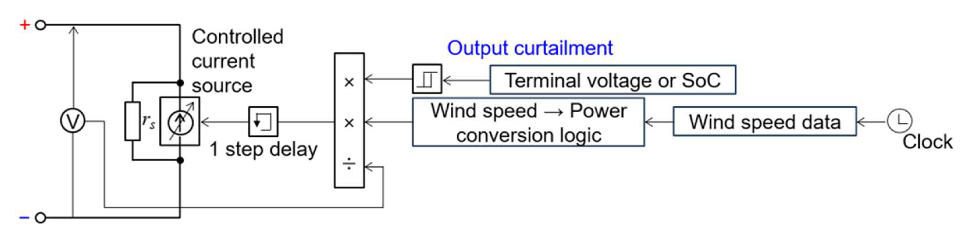
Figure A2 shows the wind-power device model. Wind-speed data are input to a logic block that converts wind speed to electrical power based on turbine specifications. This power is multiplied by a curtailment flag (1 or 0 depending on battery SoC) and divided by the device terminal voltage. The resulting value is applied to the control terminal of a controlled current source, which outputs the corresponding current at the device terminals.
Figure A2.
Wind-power generation device model.
Appendix A.3. Power Load Devices
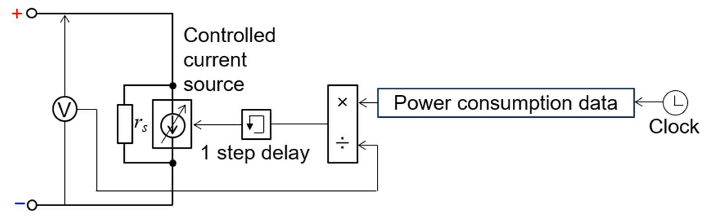
Figure A3 presents the device model for residential loads and EV charging. Load-profile data—generated from statistical residential consumption patterns and scheduled EV charging—are divided by the device terminal voltage and applied to a controlled current source. The resulting current flows into the device terminals, representing power consumption.
Figure A3.
Power load device model.
Appendix A.4. Battery-Driven DC/DC Converter Power Supply
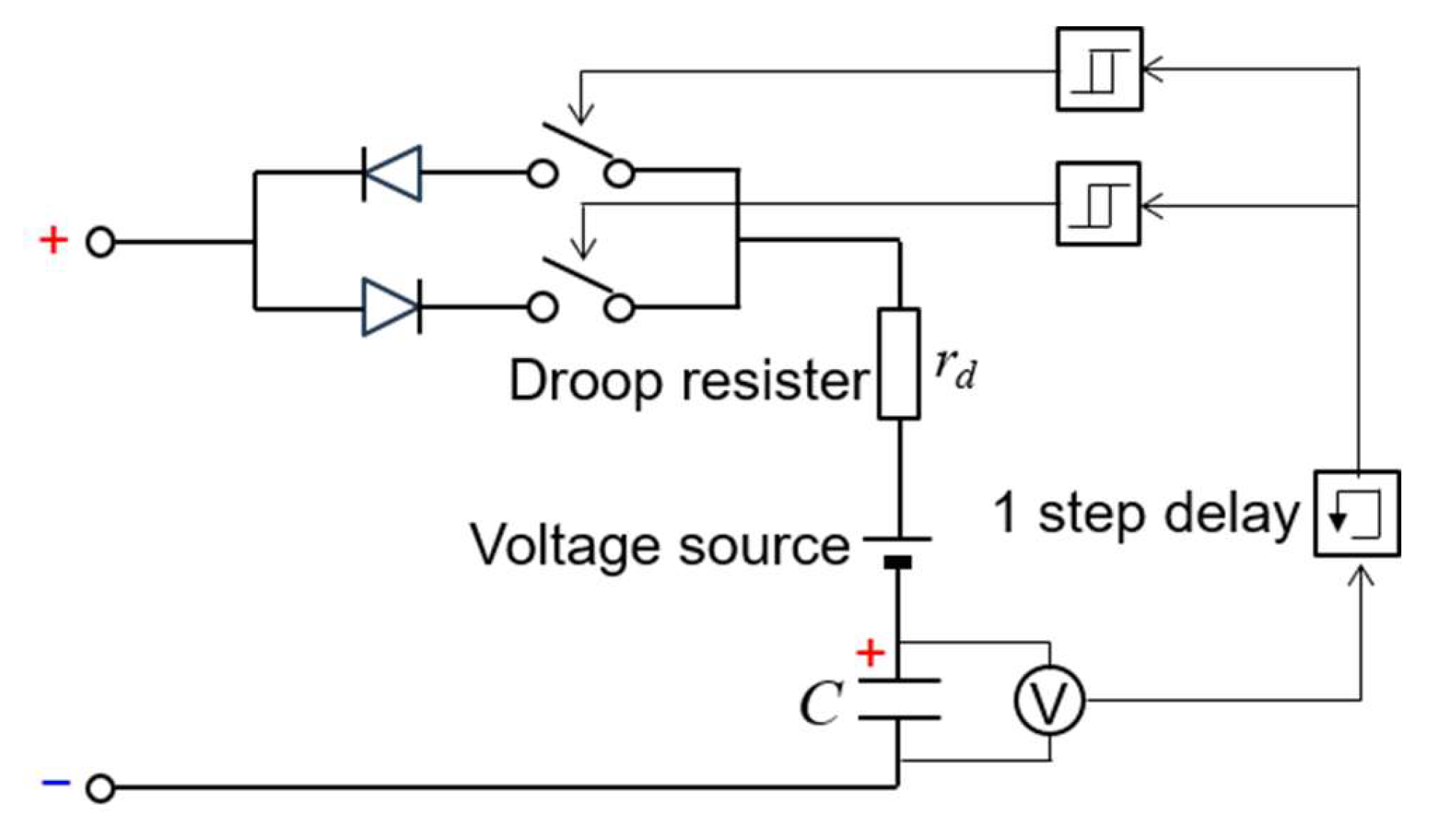
Figure A4 illustrates the battery-driven DC/DC converter model. The capacitor C represents an ideal large-capacitance element whose stored charge (proportional to its terminal voltage) is mapped to battery SoC. Based on this SoC-derived voltage, the internal voltage source is switched on or off using a hysteresis controller to maintain the prescribed feeder voltage. The series resistance rₑ provides a droop characteristic, causing terminal voltage to decrease with increasing output current.
Figure A4.
Battery-driven DC/DC converter device model.
Appendix A.5 LiFePO₄ Battery Model
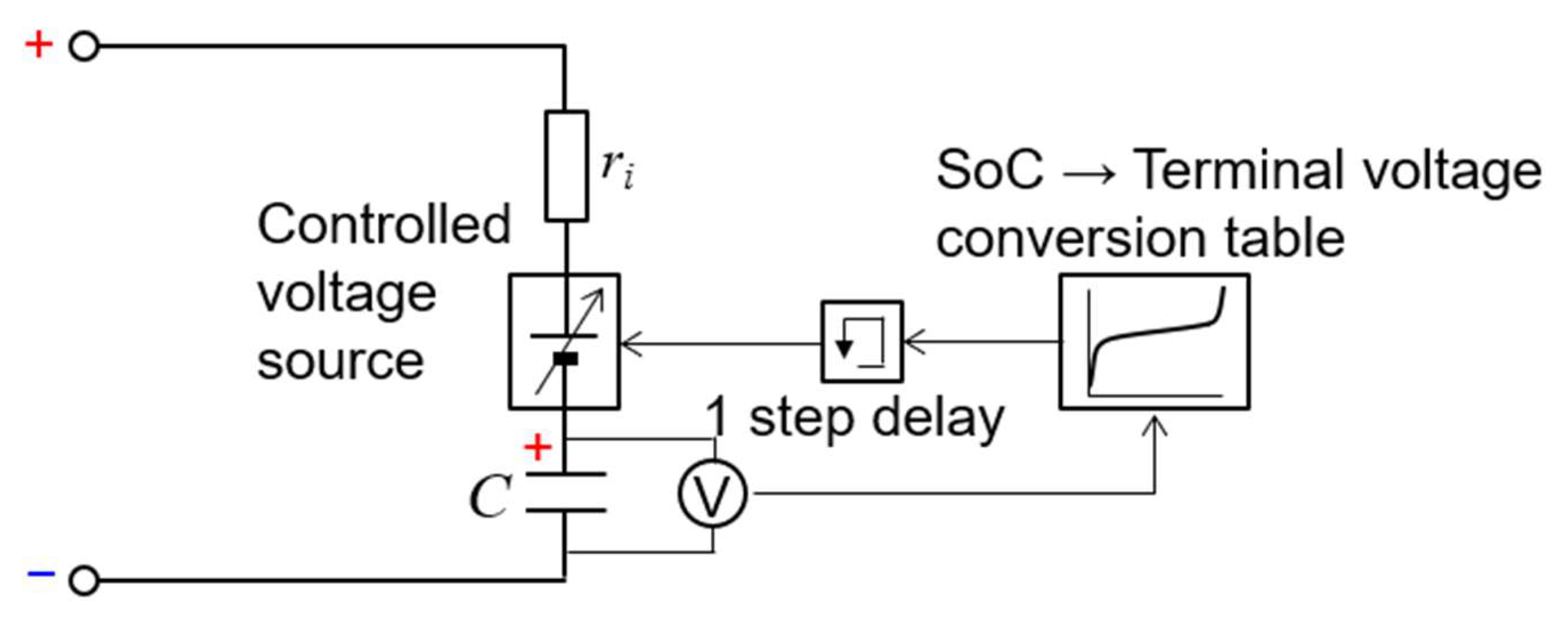
Figure A5 shows the LiFePO₄ battery device model. The capacitor C represents stored charge, and its terminal voltage is converted to battery terminal voltage using a lookup table representing the battery’s charge/discharge characteristics. The resulting voltage drives a controlled voltage source. The internal resistance rᵢ is set inversely proportional to battery capacity.
Figure A5.
LiFePO₄ battery device model.
Appendix A.6. Grid Power-Exchange Unit
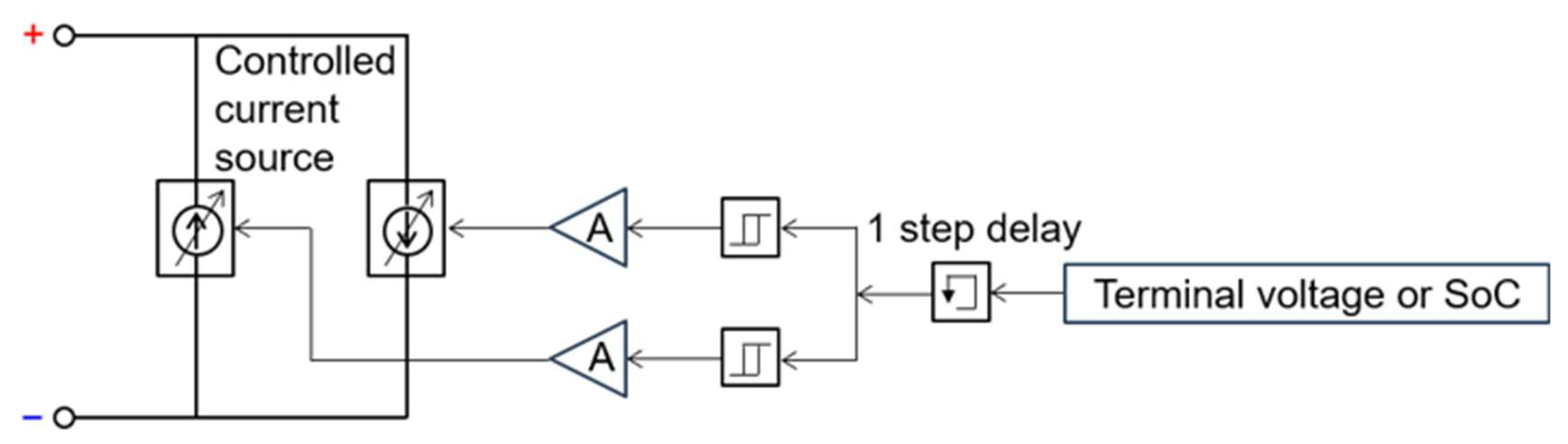
Figure A6 illustrates the device model for bidirectional power exchange with the utility grid. Based on device terminal voltage and battery SoC, two controlled current sources—connected in opposite directions—are individually activated to perform import or export. Parameter A specifies the exchange current.
Figure A6.
Grid power-exchange device model.
References
- Weniger, J.; Tjaden, T.; Quaschning, V. Sizing of Residential PV Battery Systems. Energy Procedia 2014, 46, 78–87. [Google Scholar] [CrossRef]
- Boeckl, B.; Kienberger, T. Sizing of PV storage systems for different household types. J. Energy Storage 2019, 24, 100763. [Google Scholar] [CrossRef]
- Dai, B.; Wang, H.; Li, B.; Li, C.; Tan, Z. Capacity model and optimal scheduling strategy of multi-microgrid based on shared energy storage. Energy 2024, 306, 132472. [Google Scholar] [CrossRef]
- Gholami, M.; Muyeen, S.M.; Lin, S. Optimizing microgrid efficiency: Coordinating commercial and residential demand patterns with shared battery energy storage. J. Energy Storage 2024, 88, 111485. [Google Scholar] [CrossRef]
- Zhang, X.; Lyu, J.; Li, Y.; Zeng, Z.; Wang, Z.; Dehghanian, P.; Tan, T. Degradation-aware optimization for shared energy storage in solar integrated microgrids. Sol. Energy 2026, 315, 114760. [Google Scholar] [CrossRef]
- Chauhan, R.K.; Chauhan, K.; Subrahmanyam, B.R.; Singh, A.G.; Garg, N.M. Distributed and centralized autonomous DC microgrid for residential buildings: A case study. J. Build. Eng. 2020, 27, 100978. [Google Scholar] [CrossRef]
- Ling, J.-M.; Mulani, F.I. Planning and optimization of a residential microgrid utilizing renewable resources and integrated energy storage. J. Energy Storage 2024, 97, 112933. [Google Scholar] [CrossRef]
- Yamada, H. Autonomous Decentralized Cooperative Control DC Microgrid Deployed in Residential Areas. Energies 2025, 18, 5041. [Google Scholar] [CrossRef]
- Ali, S.; Zheng, Z.; Aillerie, M.; Sawicki, J.-P.; Péra, M.-C.; Hissel, D. A Review of DC Microgrid Energy Management Systems Dedicated to Residential Applications. Energies 2021, 14, 4308. [Google Scholar] [CrossRef]
- Wei, Q.; Liu, D.; Lewis, F.L.; Liu, Y.; Zhang, J. Mixed Iterative Adaptive Dynamic Programming for Optimal Battery Energy Control in Smart Residential Microgrids. IEEE Trans. Ind. Electron. 2017, 64, 4110–4120. [Google Scholar] [CrossRef]
- Atef, M.; Alahakoon, S.; Wolfs, P.; Mumtahina, U.; Khatib, T.; Uddin, M. Energy Management in Microgrids: Commercial, Industrial, and Residential Perspectives. Energies 2026, 19, 419. [Google Scholar] [CrossRef]
- Kakigano, H.; Miura, Y.; Ise, T.; Momose, T.; Hayakawa, H. Fundamental characteristics of DC microgrid for residential houses with cogeneration system in each house. In IEEE Power and Energy Society General Meeting - Conversion and Delivery of Electrical Energy in the 21st Century; Pittsburgh, PA, USA, 2008; pp. 1–8. [Google Scholar] [CrossRef]
- Masango, F.I.; Jordaan, J.; Nnachi, A.F. Modeling and Analysis of Residential DC Microgrid Energy Management Using System of Systems Architecture. IEEE AFRICON 2023, 1–6. [Google Scholar] [CrossRef]
- Alarcón, M.A.; Alarcón, R.G.; González, A.H.; Ferramosca, A. Modeling a residential microgrid for energy management. Argentine Conference on Automatic Control, Buenos Aires, Argentina, 2020; pp. 1–6. [Google Scholar] [CrossRef]
- Hurtt, J.; Mili, L. Residential microgrid model for disaster recovery operations. IEEE Grenoble Conference, Grenoble, France, 2013; pp. 1–6. [Google Scholar] [CrossRef]
- Cai, W.; Kordabad, A.B.; Gros, S. Energy management in residential microgrid using model predictive control-based reinforcement learning and Shapley value. Eng. Appl. Artif. Intell. 2023, 119, 105793. [Google Scholar] [CrossRef]
- Ramadan, R.; Huang, Q.; Zalhaf, A.S.; Bamisile, O.; Li, J.; Mansour, D.-E.A.; Lin, X.; Yehia, D.M. Energy Management in Residential Microgrid Based on Non-Intrusive Load Monitoring and Internet of Things. Smart Cities 2024, 7, 1907–1935. [Google Scholar] [CrossRef]
- Nesihath, M.K.; Nafeesa, K.; Sreedharan, S.; Sulthan, S.M.; Satheesh, R.; Kolhe, M.L. Design and implementation of energy management system for optimal hybrid residential microgrid. Electr. Eng. 2026, 108, 52. [Google Scholar] [CrossRef]
- Winkens, A.; Contu, I.; Linnartz, P.; Ulbig, A. Experimental Validation of the Parallel Operation of Grid-Forming Converters and Synchronous Generators in Temporary Islanded Microgrids. Int. Conf. Smart Energy Syst. Technol. (SEST) 2022, 1–6. [Google Scholar] [CrossRef]
- Shuai, Z.; Huang, W.; Shen, C.; Ge, J.; Shen, Z.J. Characteristics and Restraining Method of Fast Transient Inrush Fault Currents in Synchronverters. IEEE Trans. Ind. Electron. 2017, 64, 7487–7497. [Google Scholar] [CrossRef]
- Lin, X.; Zamora, R.; Sheina, A. A Comprehensive Review of DC Microgrids: Controls, Topologies, Protection and Future Trends. Fractal Fract. 2026, 10, 396. [Google Scholar] [CrossRef]
- Pires, V.F.; Pires, A.; Cordeiro, A. DC Microgrids: Benefits, Architectures, Perspectives and Challenges. Energies 2023, 16, 1217. [Google Scholar] [CrossRef]
- Unamuno, E.; Andoni, J.A. Hybrid ac/dc microgrids—Part I: Review and classification of topologies. Renewable Sustain. Energy Rev. 2015, 52, 1251–1259. [Google Scholar] [CrossRef]
- Rai, I.; Suchetha, C. Microgrid and grid synchronization: A critical analysis of challenges and opportunities. Electr. Power Syst. Res. 2025, 242, 111434. [Google Scholar] [CrossRef]
- Bidram, A.; Reno, M. J.; Abadi, S.A.G.K.; Aparicio, M.J.; Bauer, D. Trends in dc microgrids: From the control and protection perspective. IEEE Electrif. Mag. 2024, 12, 33–47. [Google Scholar] [CrossRef]
- Moussa, M.; Ghorbal, M.J.-B.; Slama-Belkhodja, I. Bus voltage level choice for standalone residential DC nanogrid. Sustain. Cities Soc. 2019, 46, 101431. [Google Scholar] [CrossRef]
- Dragicevic, T.; Lu, X.; Vasquez, J.C.; Guerrero, J.M. DC Microgrids—Part II: A Review of Power Architectures, Applications, and Standardization Issues. IEEE Trans. Power Electron. 2016, 31, 3528–3549. [Google Scholar] [CrossRef]
- Hossain, M.S.; Hossain, M.A.; Oo, A.M.T. A critical review on control mechanisms, supporting measures, and monitoring systems of microgrids considering large scale integration of renewable energy sources. Energy Rep. 2023, 10, 4582–4603. [Google Scholar] [CrossRef]
- Gamage, G.D.H.C.; Gamini, S.D.; Ekanayake, J.B. Reliability analysis of microgrids: Evaluation of centralized and decentralized control approaches. Electr. Power Compon. Syst. 2023, 51, 2319–2338. [Google Scholar] [CrossRef]
- Al-Ismail, F.S. DC Microgrid Planning, Operation, and Control: A Comprehensive Review. IEEE Access 2021, 9, 36154–36172. [Google Scholar] [CrossRef]
- Cañizares, C.A.; Palma-Behnke, R.; Olivares, D.E.; Mehrizi-Sani, A.; Etemadi, A.H.; Iravani, R.; Kazerani, M.; Hajimiragha, A.H.; Gomis-Bellmunt, O.; Saeedifard, M.; et al. Trends in Microgrid Control. IEEE Trans. Smart Grid 2014, 5, 1905–1919. [Google Scholar] [CrossRef]
- Meng, L.; Shafiee, Q.; Trecate, G.F.; Karimi, H.; Fulwani, D.; Lu, X.; Guerrero, J.M. Review on Control of DC Microgrids and Multiple Microgrid Clusters. IEEE J. Emerg. Sel. Top. Power Electron. 2017, 5, 928–948. [Google Scholar] [CrossRef]
- Dragiˇcevi´c, T.; Lu, X.; Vasquez, J.C.; Guerrero, J.M. DC Microgrids—Part I: A Review of Control Strategies and Stabilization Techniques. IEEE Trans. Power Electron. 2015, 31, 4876–4891. [Google Scholar] [CrossRef]
- Liu, K.; Yamada, H.; Iwatsuki, K.; Otsuji, T. Experimental Verification and Simulation Analysis of a Battery Directly Connected DC-Microgrid System. Int. J. Electr. Electron. Eng. Telecommun. 2023, 12, 326–333. [Google Scholar] [CrossRef]
- Yamada, H. Autonomous Decentralized Cooperative Control DC Microgrids Realized by Directly Connecting Batteries to the Baseline. Electronics 2025, 14, 1356. [Google Scholar] [CrossRef]
- Japan Meteorological Agency (JMA). Historical Solar Irradiance and Meteorological Data. Available online: https://www.data.jma.go.jp/obd/stats/etrn/index.php.
- . [CrossRef]
- Cao, Z.; Gao, W.; Fu, Y.; Turchiano, C.; Vosoughi Kurdkandi, N.; Gu, J.; Mi, C. Second-Life Assessment of Commercial LiFePO4 Batteries Retired from EVs. Batteries 2024, 10, 306. [Google Scholar] [CrossRef]
- Yang, Z.; Li, X.; Li, J.; Li, H.; Shi, J.; Fan, X.; Cong, Z.; Feng, X.; Yang, X.-G. Study on Influencing Factors of Calendar Aging and Cycle Aging of LFP Batteries. Appl. Sci. 2025, 15, 12749. [Google Scholar] [CrossRef]
- Vachenauer, V.; Karger, A.; Naumann, M.; Durdel, A.; Jossen, A. Shelf life of lithium-ion batteries: Recommissioning LiFePO4/C cells after ten years of uninterrupted calendar aging. J. Power Sources 2025, 654, 237779. [Google Scholar] [CrossRef]
- GitHub. Available online: https://github.com/hiro1959/dc-microgrid-simulator.
Figure 1.
Conceptual configuration of autonomous distributed cooperative control.
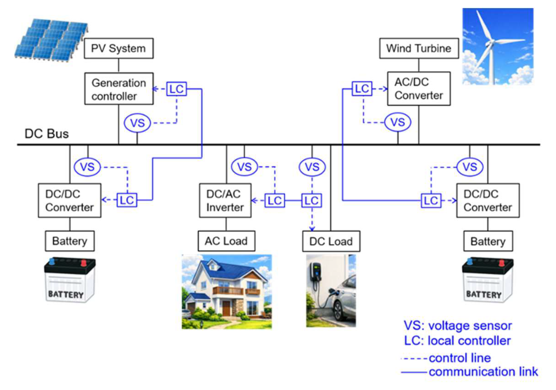
Figure 2.
Conceptual configuration of autonomous decentralized control.
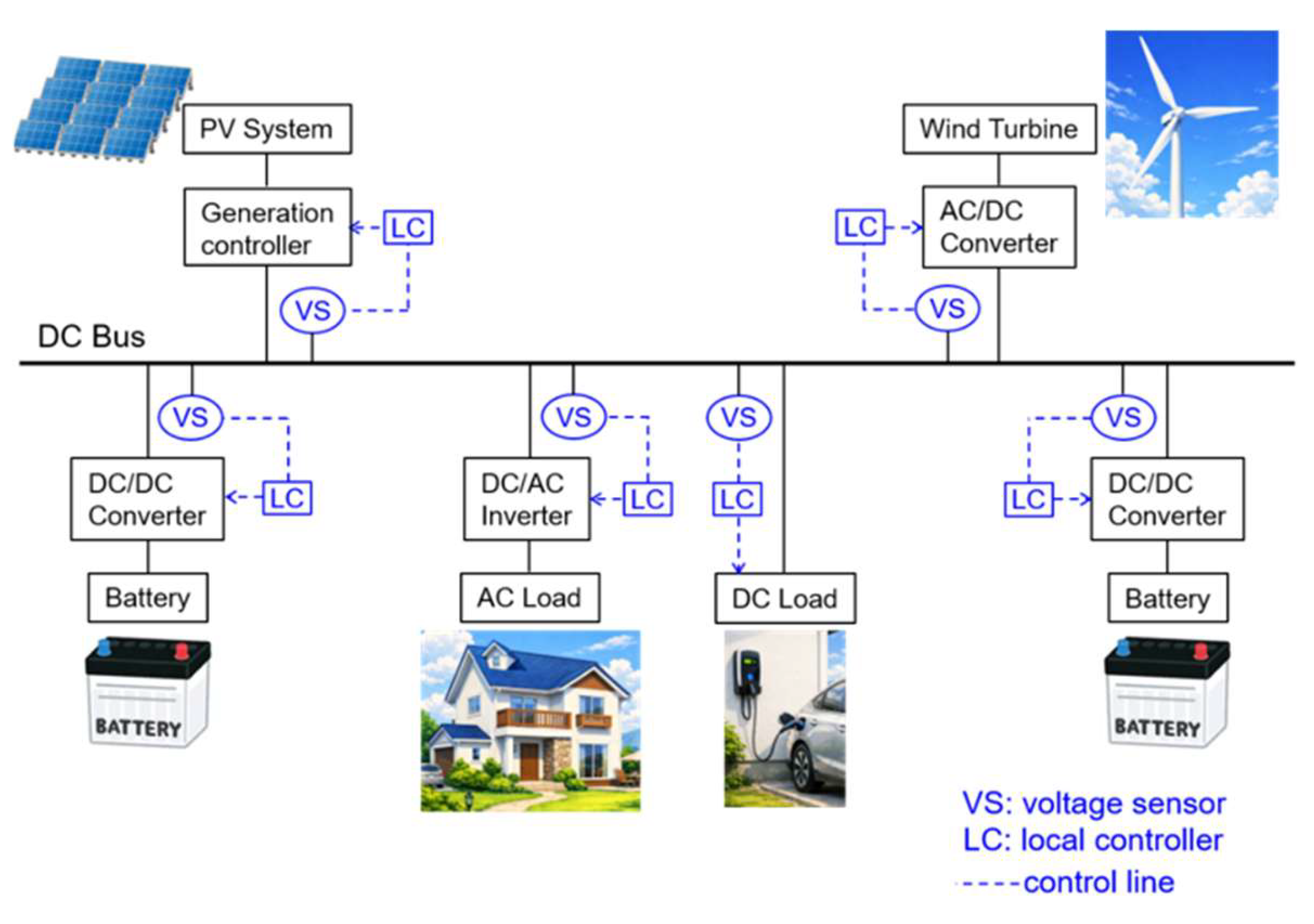
Figure 3.
Conceptual configuration of the modeled residential DC microgrid.
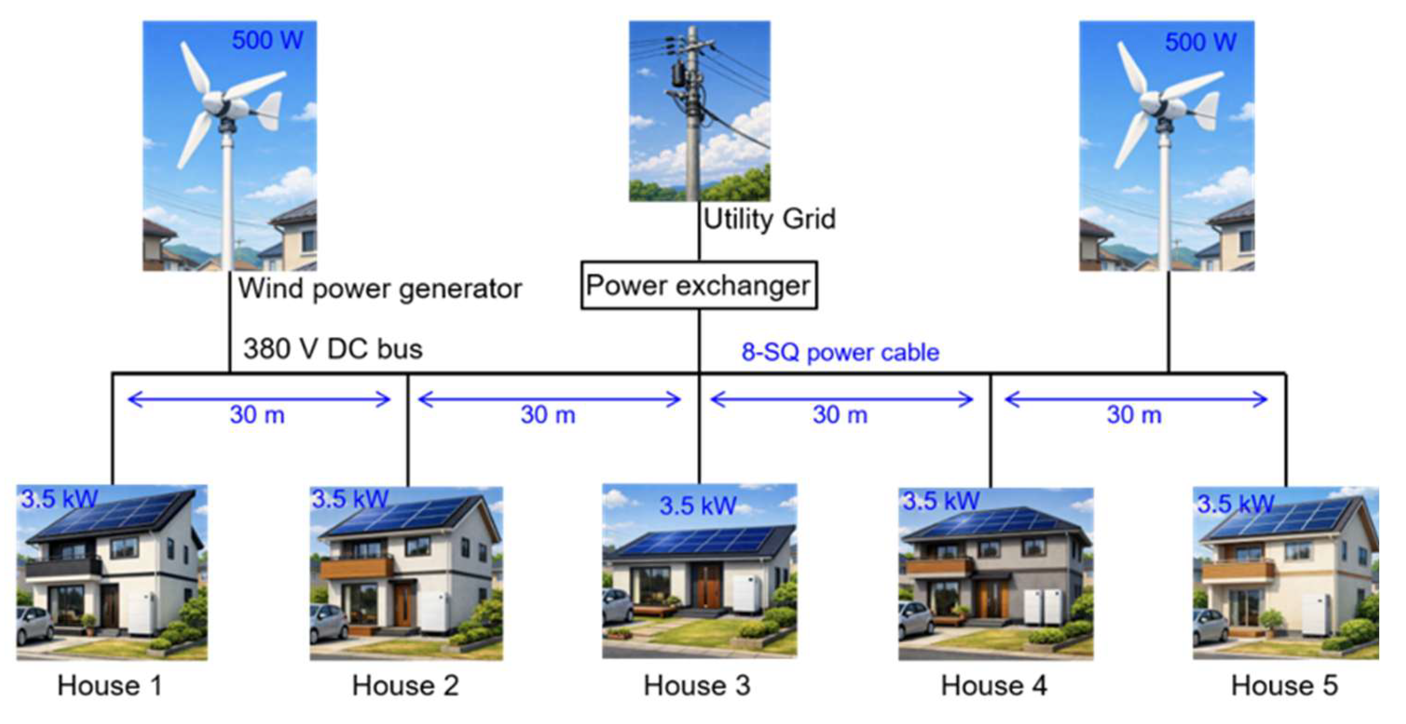
Figure 4.
Simulation interface of the residential DC microgrid under autonomous distributed cooperative control.
Figure 4.
Simulation interface of the residential DC microgrid under autonomous distributed cooperative control.
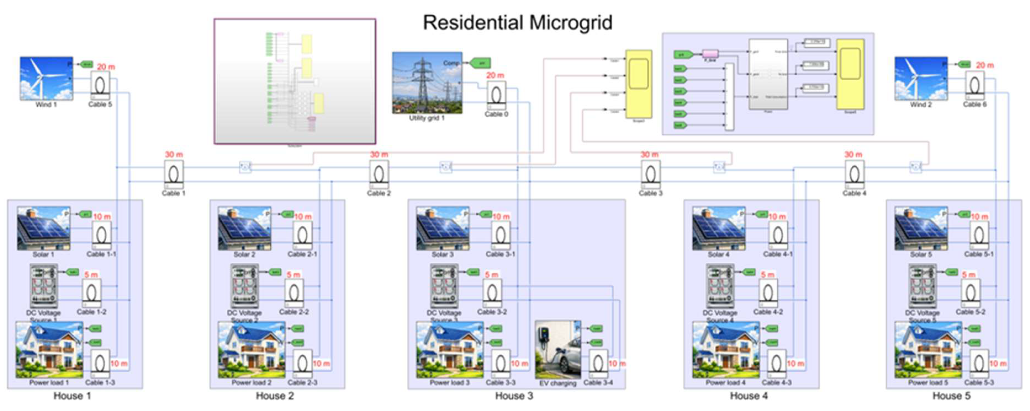
Figure 5.
Annual voltage profiles at various points in the microgrid.
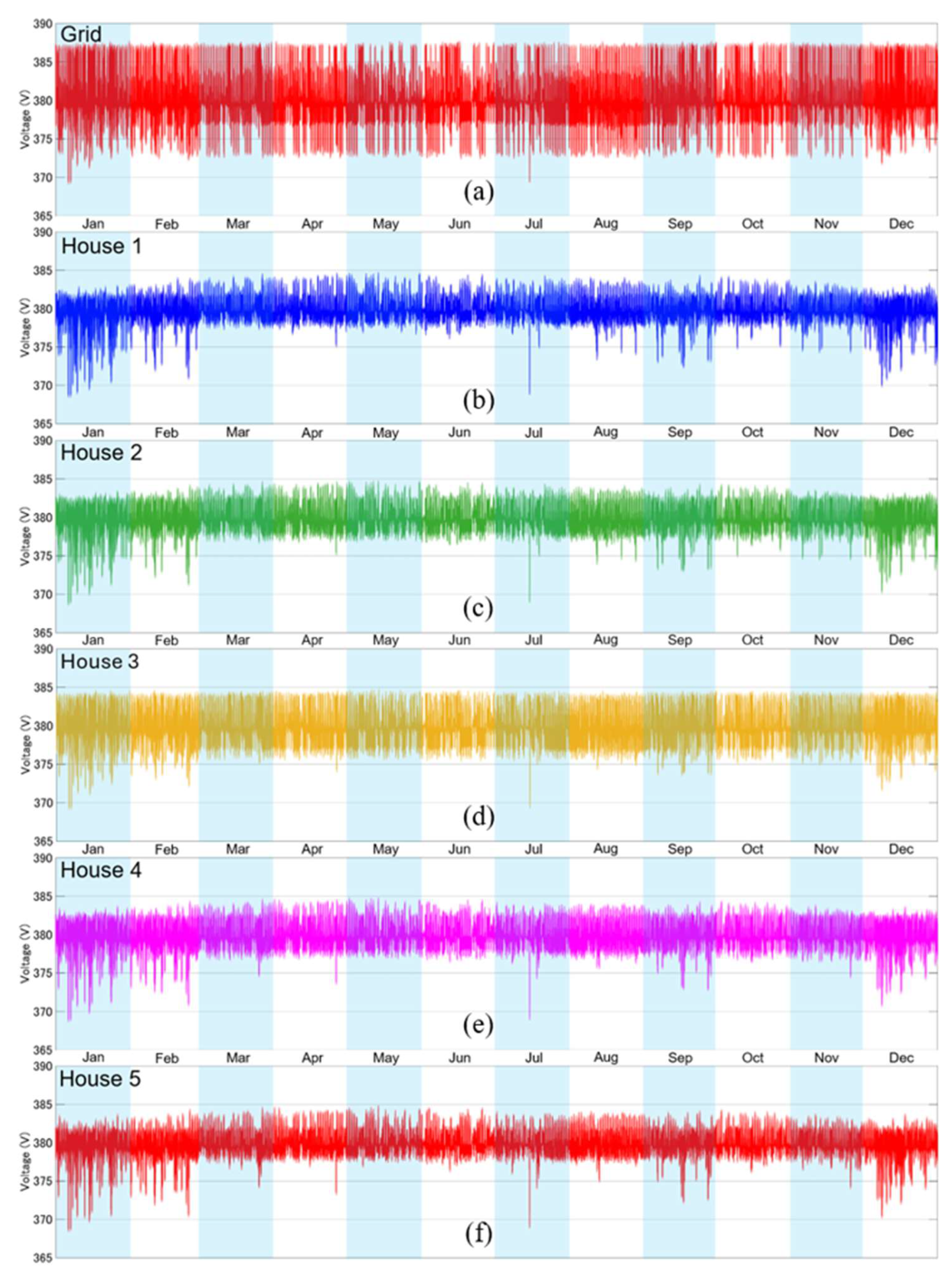
Figure 6.
Annual PV generation profiles.
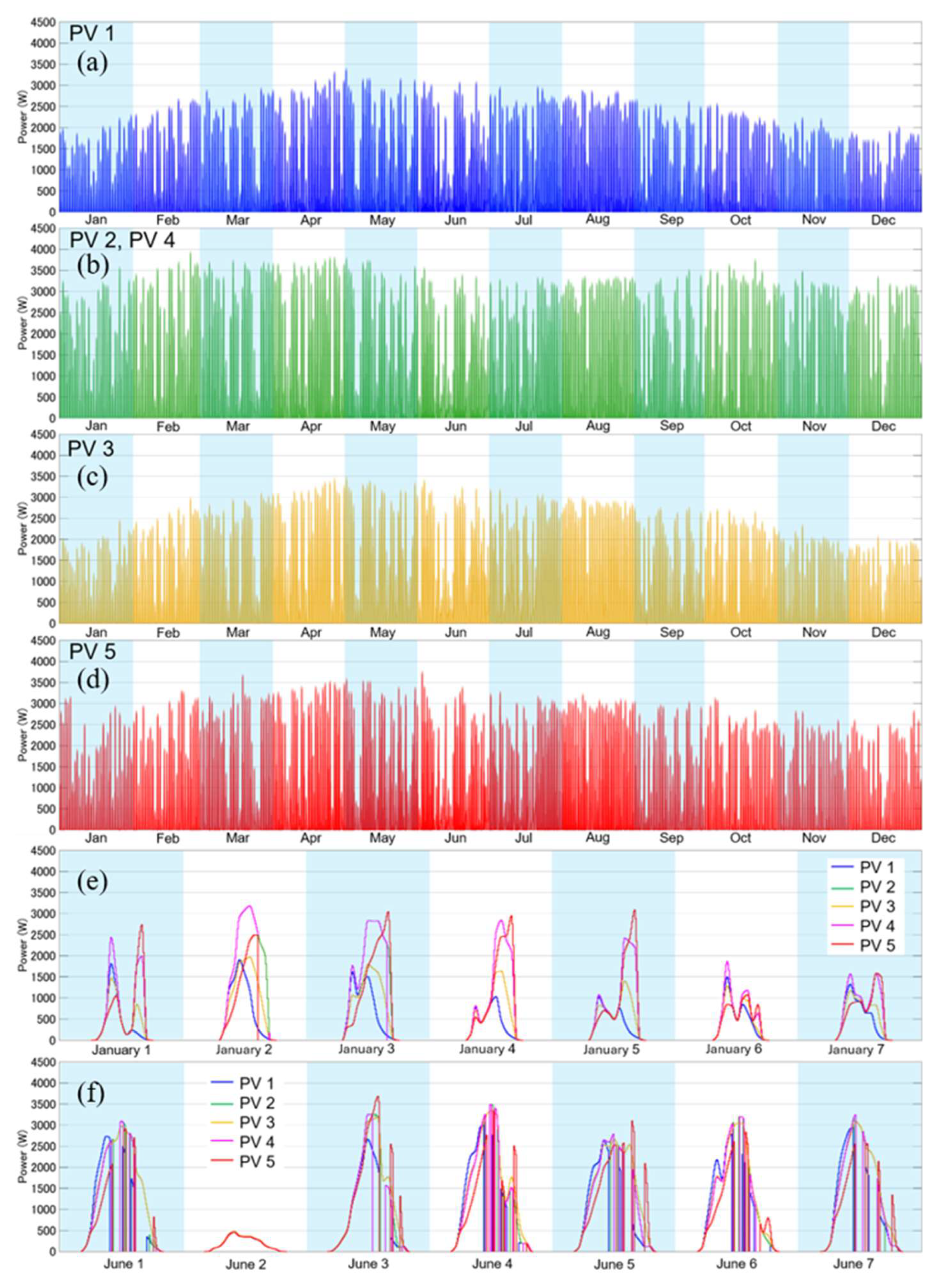
Figure 7.
Annual wind-power generation profiles.
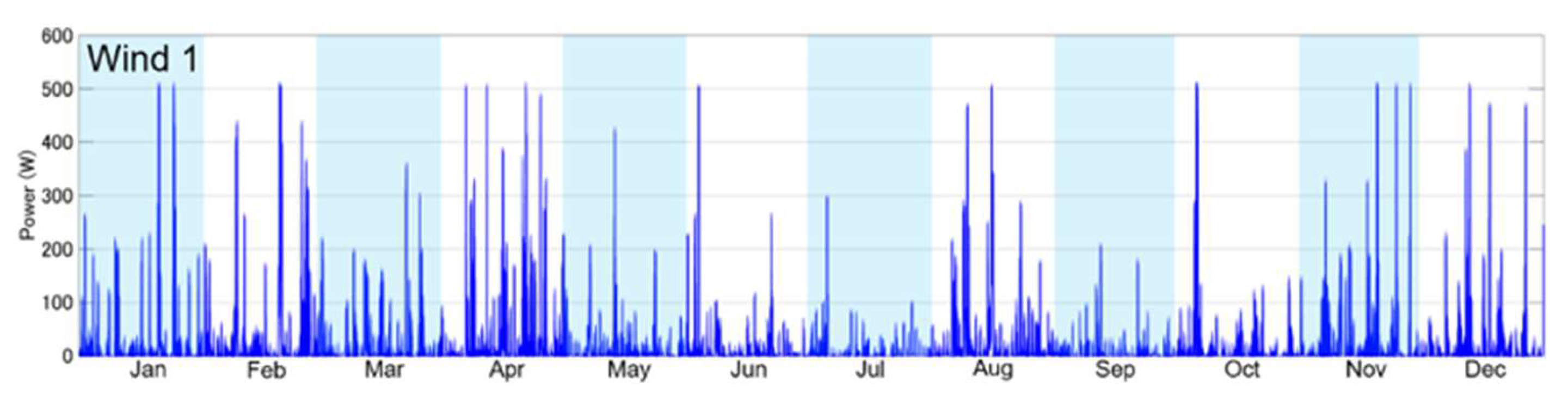
Figure 8.
Annual household electricity consumption profiles.
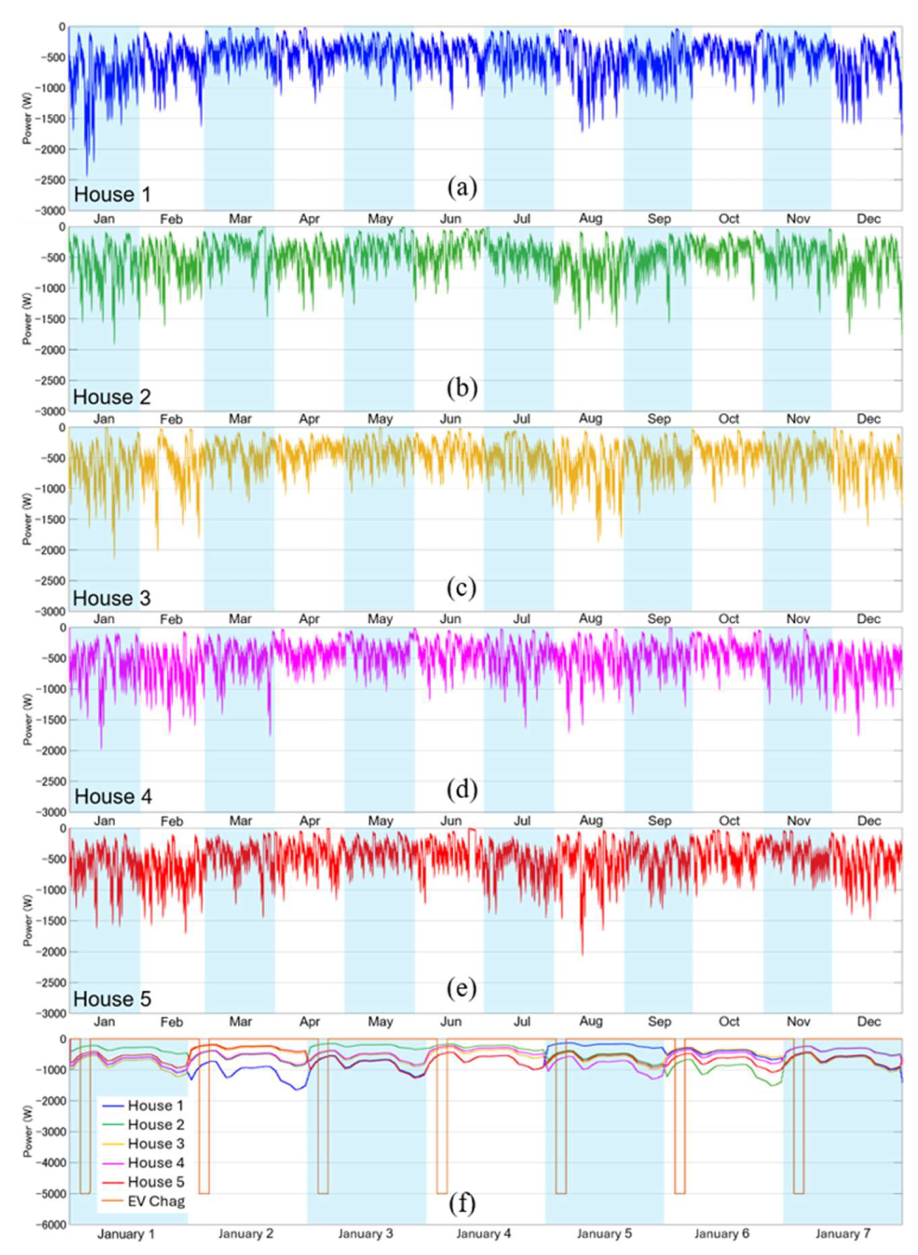
Figure 9.
Annual current profiles along the feeder cable.
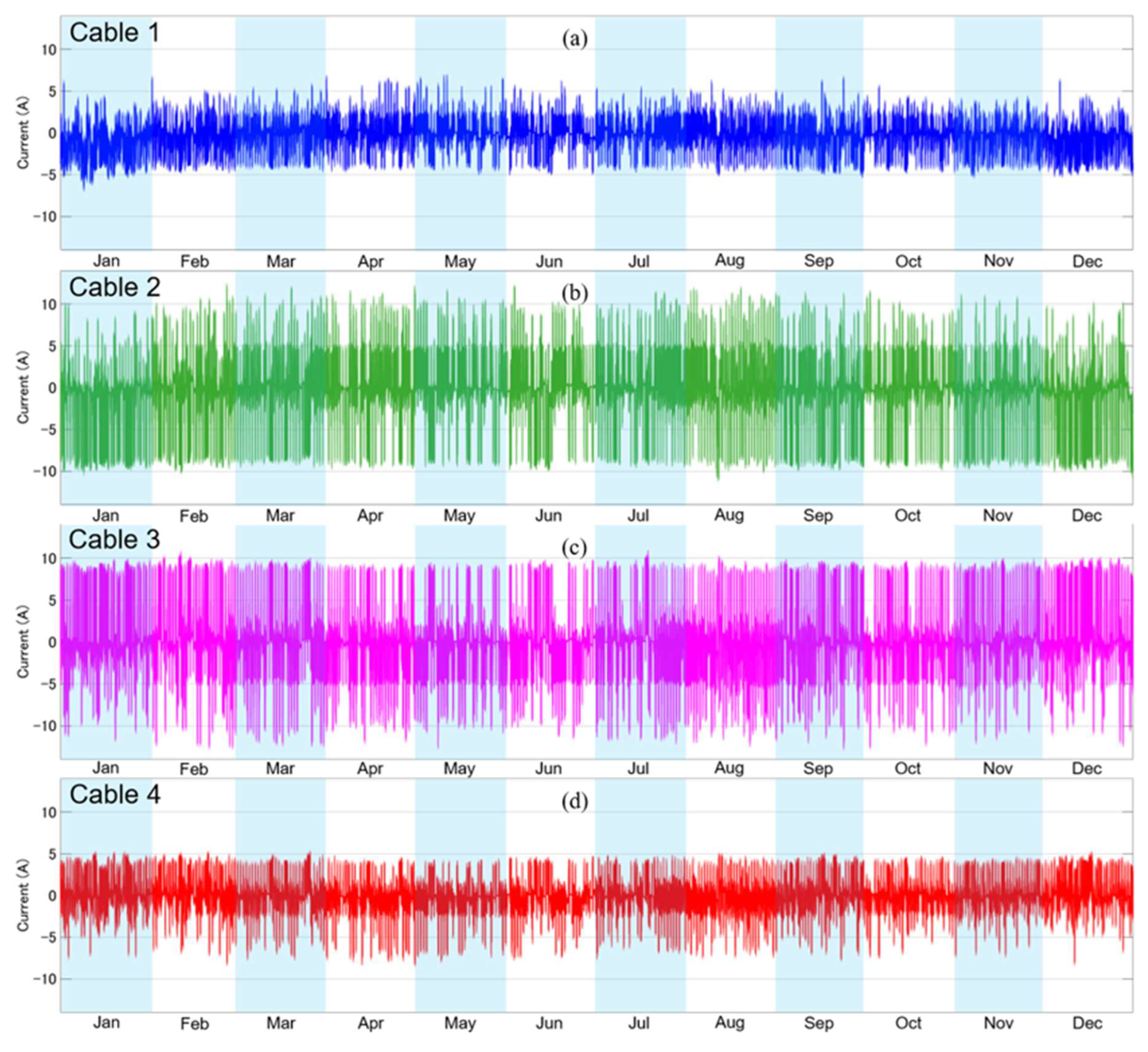
Figure 10.
Annual SoC profiles of the battery-driven power sources.
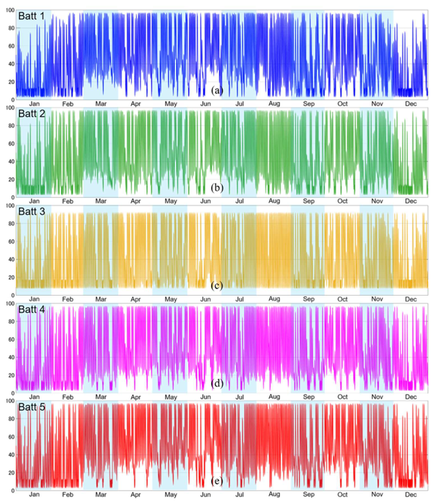
Figure 11.
Cumulative household consumption, grid import, and grid export.
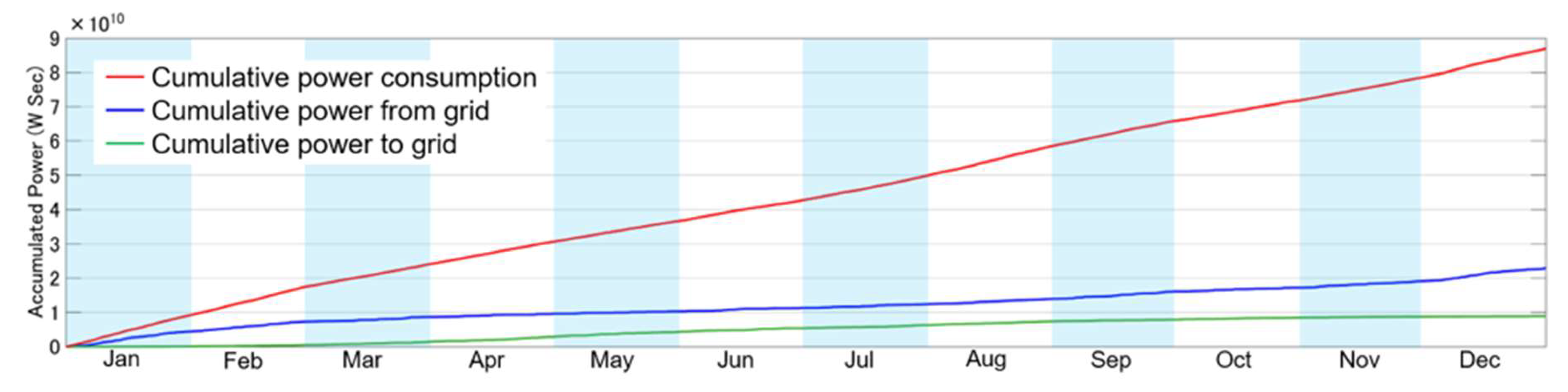
Figure 12.
Annual cumulative charge/discharge current of each battery-driven power source.
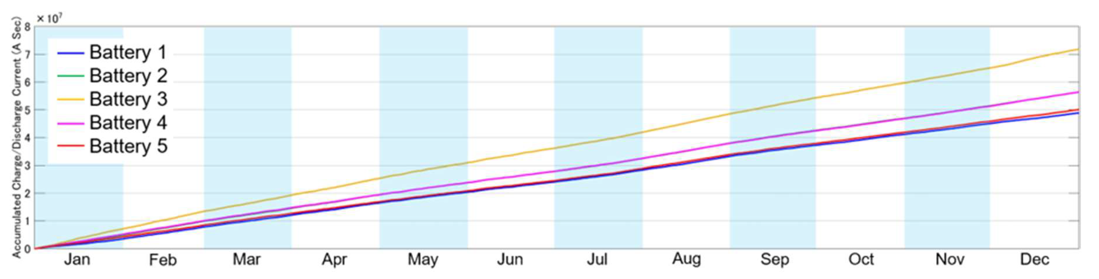
Figure 13.
Simulation interface of the residential DC microgrid under autonomous decentralized control.
Figure 13.
Simulation interface of the residential DC microgrid under autonomous decentralized control.
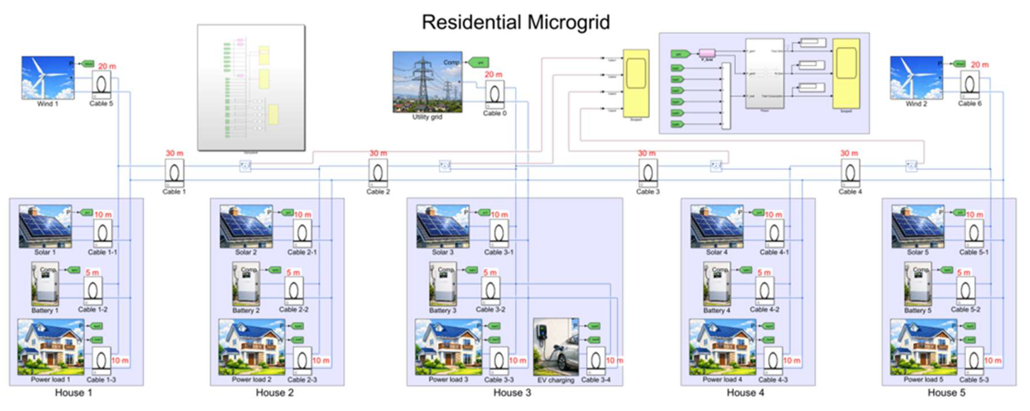
Figure 14.
Annual voltage profiles at various points in the microgrid.
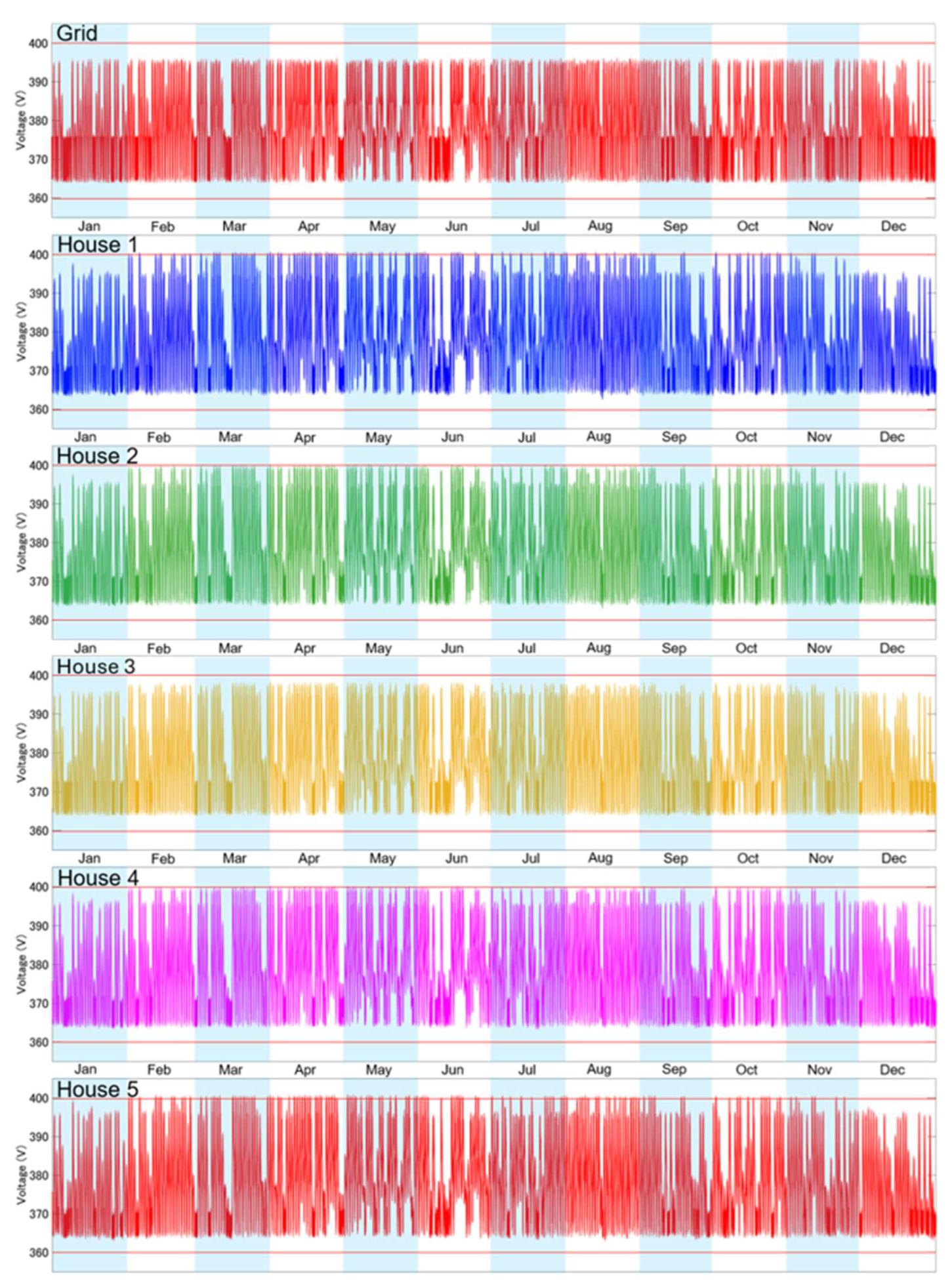
Figure 15.
Cumulative household consumption, grid import, and grid export.
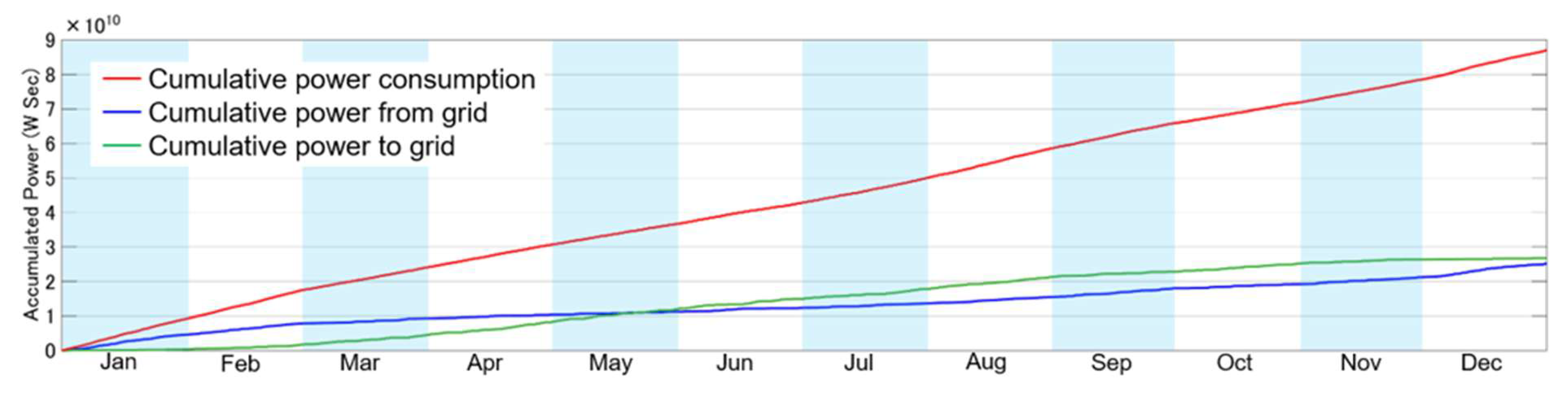
Figure 16.
Annual cumulative charge/discharge current of each battery.
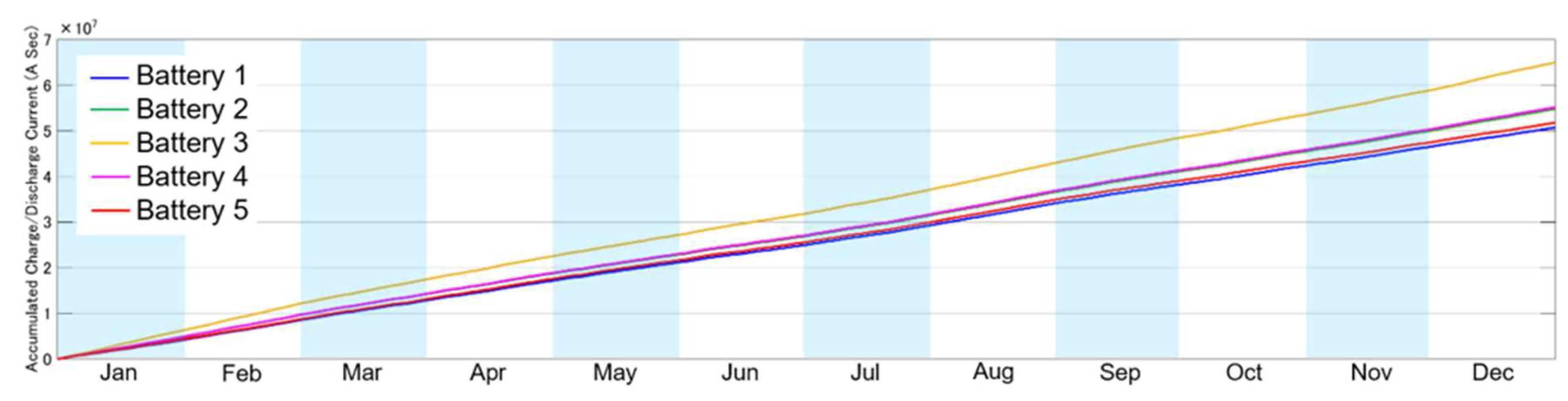
Figure 17.
Dependence of grid import/export on battery capacity (autonomous distributed cooperative control).
Figure 17.
Dependence of grid import/export on battery capacity (autonomous distributed cooperative control).
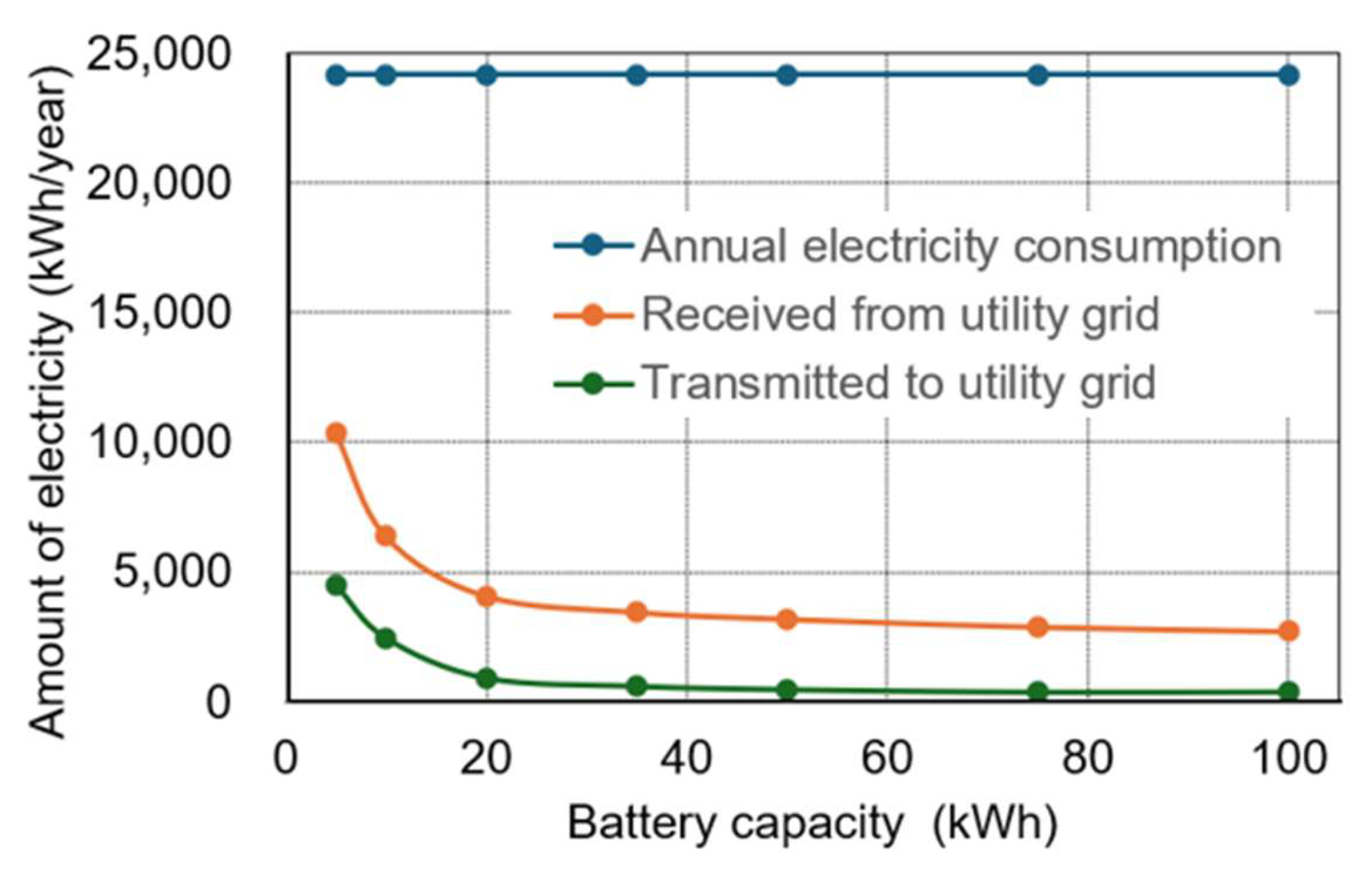
Figure 18.
Dependence of grid import/export on battery capacity (autonomous decentralized control).
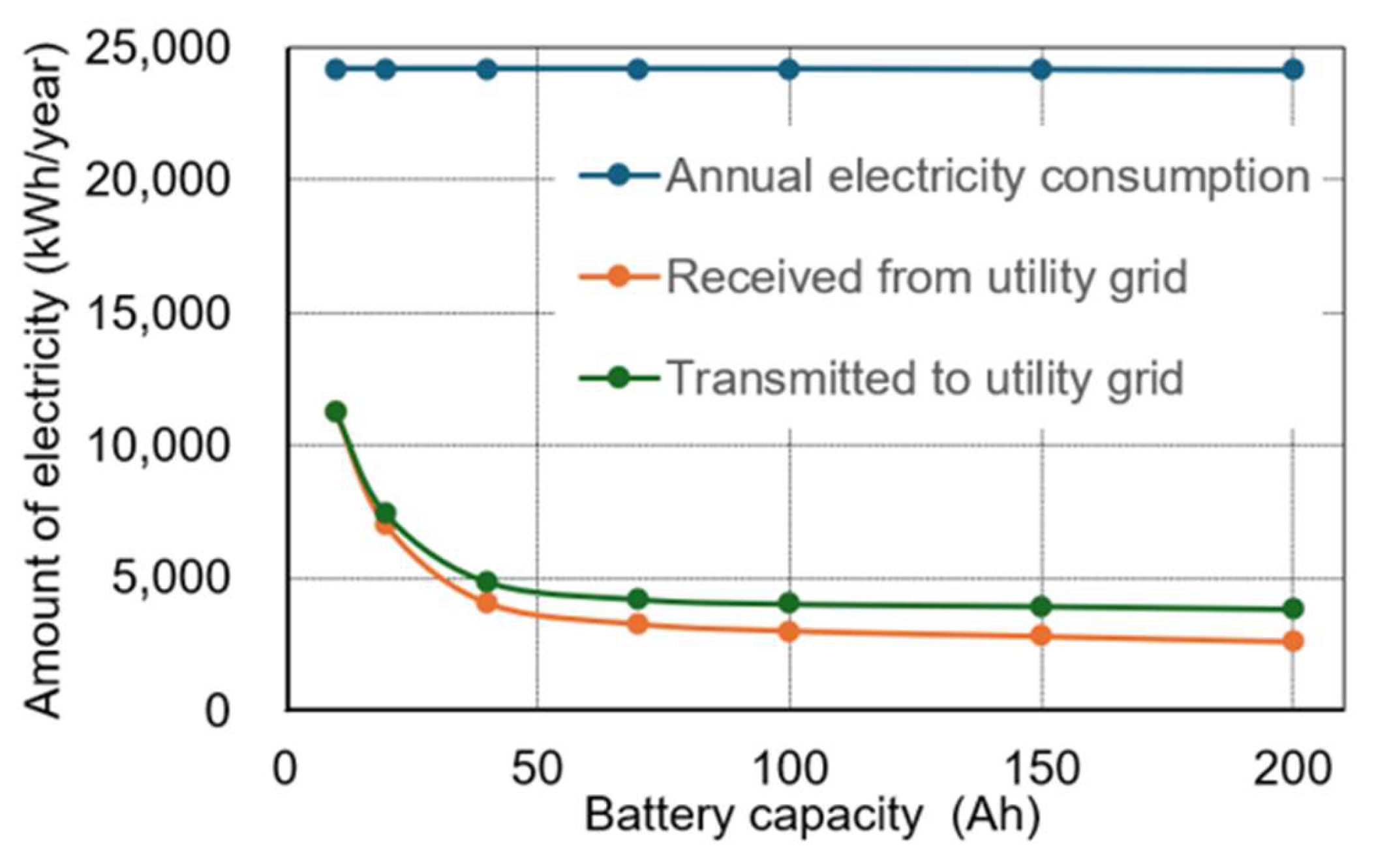
Figure 19.
Off-grid operation: (a) autonomous distributed cooperative control, (b) autonomous decentralized control.
Figure 19.
Off-grid operation: (a) autonomous distributed cooperative control, (b) autonomous decentralized control.
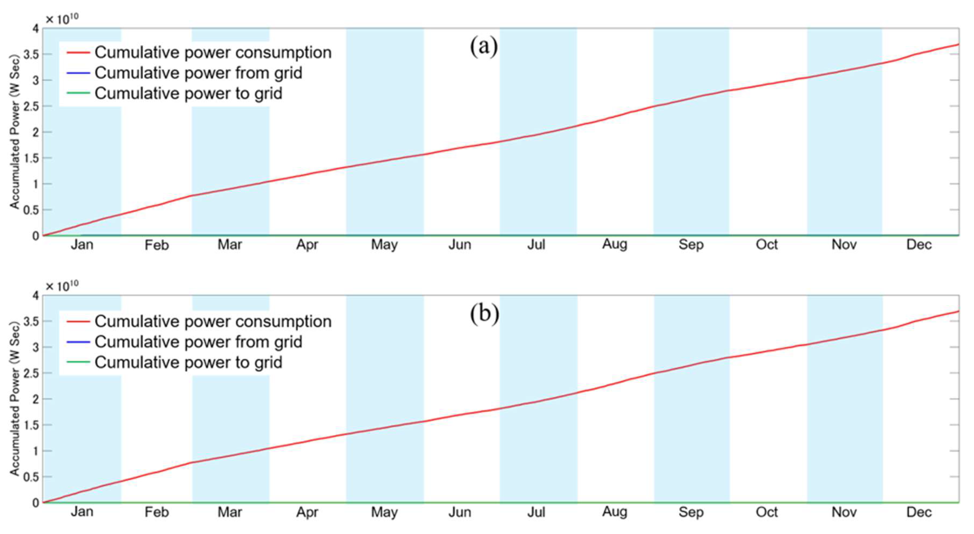

Table 1.
Specifications of the autonomous distributed cooperative control microgrid model.
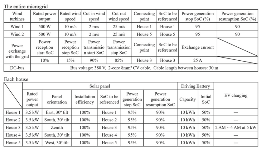 |
Table 2.
Specifications of the autonomous decentralized control microgrid model.
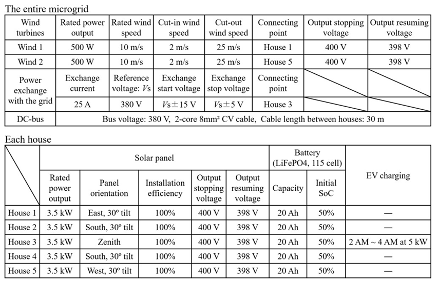 |
Table 3.
Dependence of grid import/export on battery capacity (autonomous distributed cooperative control).
Table 3.
Dependence of grid import/export on battery capacity (autonomous distributed cooperative control).
| Battery Capacity (kWh) | Annual Electricity Consumption (kWh) | Received from the Utility Grid (kWh) | Transmitted to the Utility Grid (kWh) |
|---|---|---|---|
| 5 | 24,180 | 10,360 | 4,525 |
| 10 | 24,180 | 6,372 | 2,471 |
| 20 | 24,180 | 4,078 | 927.2 |
| 35 | 24,180 | 3,461 | 612.5 |
| 50 | 24,180 | 3,197 | 482.8 |
| 75 | 24,180 | 2,897 | 384.7 |
| 100 | 24,180 | 2,725 | 392.8 |
Table 4.
Dependence of grid import/export on battery capacity (autonomous decentralized control).
| Battery Capacity (Ah) | Annual Electricity Consumption (kWh) | Received from the Utility Grid (kWh) | Transmitted to the Utility Grid (kWh) |
|---|---|---|---|
| 10 | 24,180 | 11,280 | 11,290 |
| 20 | 24,180 | 7,006 | 7,442 |
| 40 | 24,180 | 4,078 | 4,875 |
| 70 | 24,170 | 3,278 | 4,211 |
| 100 | 24,170 | 3,019 | 4,039 |
| 150 | 24,150 | 2,814 | 3,950 |
| 200 | 24,130 | 2,611 | 3,844 |
Disclaimer/Publisher’s Note: The statements, opinions and data contained in all publications are solely those of the individual author(s) and contributor(s) and not of MDPI and/or the editor(s). MDPI and/or the editor(s) disclaim responsibility for any injury to people or property resulting from any ideas, methods, instructions or products referred to in the content. |
© 2026 by the authors. Licensee MDPI, Basel, Switzerland. This article is an open access article distributed under the terms and conditions of the Creative Commons Attribution (CC BY) license (http://creativecommons.org/licenses/by/4.0/).
Copyright: This open access article is published under a Creative Commons CC BY 4.0 license, which permit the free download, distribution, and reuse, provided that the author and preprint are cited in any reuse.