
Submitted:
29 August 2026
Posted:
31 August 2026
You are already at the latest version
Abstract
A decline in CO₂ emissions is often treated as evidence of successful climate policy, although the same outcome may reflect technological modernization, economic contraction, demographic decline, deindustrialization, or external shocks. This study develops a three-stage diagnostic framework combining additive Logarithmic Mean Divisia Index (LMDI) decomposition, sectoral carbon cost exposure, and an investment-capacity proxy to distinguish managed decarbonization from carbon-intensive decoupling and structural or shock-driven emissions decline. The framework is applied to Germany, Poland, and Ukraine for 1990-2024, with subperiods reflecting major structural transformations and shocks. Germany reduced emissions by 482.48 Mt CO₂ despite rising population and GDP per capita, as lower energy- and carbon-intensity more than offset these upward pressures. Poland reduced emissions by 103.48 Mt CO₂, through energy-intensity improvements, while carbon-intensity gains were more limited. Ukraine recorded the largest decline (564.03 Mt CO₂), but substantial contributions came from lower GDP per capita and population, while carbon-intensity increased emissions over the period. At a common benchmark of EUR 75.28/tCO₂, Ukraine has the highest exposure among the integrated-steel cases, whereas Poland has the highest exposure among the electricity cases. The findings show that emissions outcomes should be interpreted jointly with their drivers, sectoral carbon-price transmission, and the capacity to finance technological response.
Keywords:
managed decarbonization
; structural emissions decline
; LMDI decomposition
; gross carbon-cost exposure
; carbon pricing
; investment capacity
; industrial modernization
1. Introduction
International comparisons of climate performance frequently emphasize the magnitude of greenhouse-gas or carbon-dioxide reductions. This outcome-based perspective is intuitively attractive, but it can conceal fundamentally different transition processes. A similar decline in CO2 may reflect technological modernization, lower energy intensity, decarbonization of the energy supply, economic contraction, deindustrialization, demographic decline, territorial disruption, or war. Emissions decline is therefore not synonymous with managed decarbonization.
In this study, managed decarbonization is defined as a sustained reduction in CO2 emissions in which improvements in aggregate energy intensity and CO2 intensity relative to primary energy play a dominant role, while economic activity is maintained or grows and the exposure and capacity evidence remains consistent with technological adaptation. Structural or shock-driven emissions decline refers to reductions dominated by lower economic activity, population loss, deindustrialization, destruction of productive assets, or other exogenous shocks. Carbon-intensive decoupling denotes an intermediate trajectory in which emissions are stabilized or reduced during economic growth mainly through lower aggregate energy intensity, while aggregate CO2 intensity relative to primary energy remains comparatively high or improves only weakly.
The terminology requires an explicit boundary. The related phrase “managed decarbonization transition” has been used for a coordinated, publicly governed phase-down of coal assets [55]. Here, managed decarbonization is a broader operational construct for evaluating national emissions trajectories; it is not presented as a universally standardized label. Decoupling describes the observed relation between emissions and economic output [5,6,7], whereas green growth additionally requires that environmental improvement accompany maintained or improving economic performance rather than recession [4]. Structural change can lower emissions through sectoral reallocation or loss of output without cleaner technology. Accordingly, “genuine decarbonization” and “decarbonization quality” are treated here as evaluative ideas: the observed decline is judged by its drivers, durability, institutional support, and capacity for technological response, using the decision rules specified in Section 2.7.
This distinction matters for sustainability assessment. A country may report a large historical emissions decline while lacking a durable low-carbon production system. Conversely, another country may achieve a smaller headline reduction while undertaking a more expensive and technologically demanding transformation. Comparative climate-policy research has therefore stressed the need for multiple metrics rather than reliance on a single outcome indicator [1,2,3]. Historical evidence also shows that periods of recession and structural crisis have frequently produced emissions reductions that should not be interpreted as green growth [4].
The decoupling literature examines whether economic growth can be separated from energy use and emissions. European evidence links stronger decoupling to energy-policy design and efficiency improvements [5], while global studies document substantial cross-country heterogeneity in both the extent and durability of decoupling [6,7]. However, conventional decoupling indicators do not fully identify the mechanism behind an observed change. Additive LMDI decomposition is particularly useful because it attributes the absolute change in emissions to population, economic activity, energy intensity, and carbon intensity without a residual term [8]. Decomposition has been combined with decoupling analysis in national studies [9,10], but it usually remains retrospective and does not assess whether future carbon-price pressure can be converted into modernization.
GDP and GDP per capita are retained in the Kaya identity because they provide consistent aggregate measures of activity across all three countries. Employment and final consumption represent related labour-market and demand-side channels: an external shock can reduce output, employment, consumption, and emissions simultaneously, whereas investment can enable emissions to fall while productive activity is preserved. GFCF (gross fixed capital formation) is therefore quantified in Stage 3 as the available cross-country investment-capacity proxy. Employment and consumption are discussed as contextual mechanisms but are not added to the accounting identity, which avoids overlap with the GDP-per-capita effect.
Carbon pricing provides an additional but incomplete perspective. Carbon taxes and emissions-trading systems can reduce emissions when firms and consumers have feasible substitution options [11,12,13,14]. Evidence from the EU Emissions Trading System (EU ETS) also shows that firm-level responses depend on allowance allocation, cost pass-through, innovation incentives, and competitiveness conditions [15,16]. Revenue use, access to capital, and complementary industrial policy may therefore condition whether a carbon price is associated with investment or with additional gross cost pressure for exposed sectors [17,18,19].
These issues are especially important for Ukraine. Its long-term emissions trajectory includes the post-Soviet transformation of the 1990s, the loss of industrial capacity after 2014, Russia’s full-scale invasion beginning in 2022, infrastructure destruction, population displacement, and changes in territorial coverage. Recent Ukrainian energy-system research has likewise shown that wartime energy-demand trajectories are strongly affected by structural shifts in the economy, changes in the composition of energy consumption, and greenhouse-gas reduction constraints [20]. At the same time, Ukraine is increasingly exposed to the EU Carbon Border Adjustment Mechanism (CBAM), while its domestic carbon price remains very low and a national emissions-trading system is still under development [21,22,23,24,25]. Existing Ukrainian studies examine low-carbon reconstruction, sectoral decarbonization pathways, and CBAM effects [26,27,28,29,30,31,32,33]. Earlier assessments of the Ukrainian metallurgical sector also emphasized the role of best available technologies in reducing energy use and environmental pressure [34]. More specifically, scenario analysis of the Ukrainian steel sector showed that Best Available Techniques (BAT) deployment can substantially reduce specific CO2 emissions, while the trajectory of absolute emissions remains dependent on production dynamics [35]. Ukrainian energy-demand studies have also demonstrated the importance of combining economy-wide and sector-specific perspectives, showing that changes in energy consumption may reflect both production dynamics and energy-efficiency improvements associated with technological modernization [36]. But a diagnostic framework that connects the historical origin of emissions decline with prospective carbon-cost pressure and investment capacity remains missing.
Investment capacity and financing the low-carbon transition. Low-carbon technologies are capital intensive, and their deployment depends not only on the volume of capital formation but also on access to external finance, perceived risk, and the cost of capital [59,60,61]. Cross-country evidence shows that financing conditions can materially change feasible transition pathways, while reviews of low-carbon innovation identify finance and policy credibility as linked barriers [59,60,61]. GFCF captures the broad economy-wide addition to fixed assets, but neither its sectoral allocation nor its financing cost. Accordingly, GFCF/CO2 is not proposed as a direct measure of climate investment but as a parsimonious macroeconomic indicator of the capital-formation base relative to the scale of the decarbonization challenge. Section 3.6 triangulates it with GFCF/GDP, real GFCF per capita, and absolute real GFCF; project- and sector-level financing measures remain a limitation.
Literature-identification approach. Because this article develops and applies a diagnostic framework rather than conducting a systematic review, the supporting literature was identified through a targeted, non-systematic search of scholarly search engines and publisher databases. Search combinations included “LMDI” or “decomposition” with “decoupling”, “carbon pricing”, “EU ETS”, “CBAM”, “investment capacity”, “gross fixed capital formation”, “climate finance”, “cost of capital”, “green investment”, “industrial competitiveness”, “Ukraine reconstruction”, “steel”, and “cement”. Backward citation checks were used to locate foundational methods and forward searches to identify recent comparative evidence; priority was given to peer-reviewed empirical studies, official statistics, and primary regulatory sources.
This article also develops the argument advanced in earlier work on multidimensional climate-policy assessment: headline indices and outcome measures can send misleading signals when their underlying constructs differ [37]. The present study moves from cross-index comparison to a driver-based assessment of the quality and sustainability of emissions decline.
The research gap is threefold. First, LMDI studies identify historical drivers but generally stop before evaluating the prospective pressure created by carbon pricing. Second, carbon-pricing studies estimate price effects or compliance burdens but rarely distinguish whether a country’s previous emissions decline was modernization-led or contraction-led. Third, macroeconomic investment indicators are seldom integrated into this interpretation, although low-carbon transformation in steel, cement, and electricity is highly capital intensive.
The aim of this study is to develop and apply a three-stage diagnostic framework for distinguishing managed decarbonization from carbon-intensive decoupling and structural or shock-driven emissions decline. The framework integrates: (i) an additive LMDI decomposition of historical CO2 change; (ii) a scenario-based assessment of indicative gross sectoral carbon-cost exposure; and (iii) multiple macroeconomic investment-capacity indicators used to compare conditions associated with a modernization response rather than output contraction.
The study addresses the following research questions:
1. How do population, GDP per capita, energy intensity, and carbon intensity contribute to emissions changes in Germany, Poland, and Ukraine across structurally distinct periods?
2. How does a common EU ETS/CBAM-equivalent carbon-price benchmark translate into different cost exposure for steel, cement clinker, and electricity?
3. How do multiple macroeconomic investment-capacity indicators condition the diagnostic interpretation of gross carbon-price exposure and the sustainability of future emissions reductions?
Two working hypotheses guide the comparative interpretation. H1: Germany will be closest to managed decarbonization, Poland will display carbon-intensive decoupling, and Ukraine will display a predominantly structural or shock-driven decline. H2: the same carbon-price benchmark will create heterogeneous indicative gross sectoral exposure, and the joint diagnostic will be consistent with greater contraction risk where several macroeconomic investment-capacity indicators are weakest. H2 is an associative diagnostic proposition and does not predict firm-level responses.
The contribution is not a new causal estimator or a validated composite index. It is a transparent diagnostic workflow that links ex post emissions accounting, ex ante carbon-cost pressure, and transition capacity. This integration is intended to reduce the risk of classifying any large emissions decline as a climate-policy success.
2. Materials and Methods
2.1. Three-Stage Diagnostic Framework
The framework consists of three analytically linked stages. Stage 1 identifies the historical factor structure of emissions change. Stage 2 converts a carbon-price signal into indicative gross sectoral exposure per unit of output. Stage 3 compares multiple macroeconomic indicators associated with the capital-formation base available for capital-intensive modernization. The three stages are interpreted jointly rather than aggregated into a single score. The theoretical link is sequential: Stage 1 establishes whether past reductions were transition- or contraction-consistent; Stage 2 measures the prospective pressure to change carbon-intensive production; and Stage 3 compares macroeconomic conditions associated with response capacity. A historical decline alone does not show future resilience, gross carbon-cost exposure alone does not reveal the likely response, and investment capacity alone does not demonstrate emissions improvement. Their joint interpretation therefore provides a structured diagnostic assessment of the quality and prospective sustainability of the trajectory without claiming a causal or composite score. The integrative contribution is therefore conditional rather than additive: convergence across the three stages can support a distinction between a growth-compatible, financeable transition and a contraction-linked decline, while divergence—for example, falling emissions combined with a weak domestic price signal and weak capital formation—prevents any one favourable indicator from being treated as sufficient evidence of a durable transition. This joint inference is not available from three isolated rankings without explicit cross-stage interpretation rules.

Table 1.
Three-stage diagnostic framework for evaluating the quality of emissions decline.
| Stage | Indicator | Analytical question | Diagnostic interpretation |
| 1. Historical factor structure | LMDI effects | Was the CO2 change driven by population and activity, or by energy- and carbon-intensity improvements? | Energy-intensity and carbon-intensity effects are consistent with a managed-transition interpretation; activity and population decline are consistent with structural or shock effects. |
| 2. Carbon pressure | Carbon-price signal and indicative gross carbon-cost exposure | How strongly does the carbon price affect a unit of output in exposed sectors? | A predictable and material signal is consistent with stronger incentives for technology substitution, while high indicative gross exposure may be consistent with competitiveness pressure. |
| 3. Transition capacity | GFCF/CO2 and alternative macroeconomic proxies plus qualitative constraints | What do the available macroeconomic proxies indicate about the capacity to finance a technological response? | Stronger indicators are consistent with a greater capacity to modernize; weaker indicators identify conditions associated with contraction, lock-in, or market-exit risk. |
The framework is diagnostic and rule based. It is not a causal model and does not assign a universal numerical decarbonization score.
2.2. Case Selection and Periodization
The cases were selected ex ante to provide observable variation in EU membership and market access, carbon-pricing institutions, industrial structure, energy mix, historical economic transition, and exposure to major external shocks. Germany and Poland permit comparison within a shared EU ETS setting but with different power mixes and capital-formation conditions, while Ukraine provides a non-EU, reconstruction- and shock-exposed case facing a strong external CBAM signal and a weak domestic price signal. No expected trajectory label was used as a selection criterion; the labels were assigned only after applying the common calculations and interpretation rules. The sample is deliberately contrasting and theory-oriented rather than representative, and no statistical inference from these three cases to a wider country population is intended.
The 1990-2024 interval is used for long-term comparison, but it is not treated as a homogeneous decarbonization period. Subperiods are defined to separate long-term structural transformation, common external shocks, and country-specific disruptions (Table 2).
The first decade after 1990 captures reunification-related restructuring in Germany, post-socialist transformation in Poland, and a more severe post-Soviet production shock in Ukraine. The 2000-2013 period represents a more stable pre-2014 trajectory. The 2015–2019 interval between the post-2014 disruption and the COVID-19 shock is retained as a separate analytical period in the LMDI decomposition to distinguish inter-shock adjustment from event-driven subperiods. The 2019-2020 interval captures the common COVID-19 shock, while 2020-2021 captures the rebound. For Ukraine, 2021-2022 represents the full-scale invasion shock and 2022-2024 represents wartime adaptation. For Germany and Poland, the same years reflect post-pandemic adjustment and the broader European energy crisis.
2.3. Data, Units, and Harmonization
The empirical analysis combines annual macroeconomic, demographic, energy, emissions, carbon-pricing, and sectoral-intensity data. Population, GDP, and gross fixed capital formation (GFCF) are drawn from internationally harmonized databases; primary energy and territorial fossil-fuel CO2 are taken from global energy and emissions datasets; and sectoral carbon-intensity benchmarks are drawn from technical and industry sources. Table 3 summarizes the variables and their roles.
To ensure complete coverage of the 1990-2024 period, several gaps in the gross fixed capital formation (GFCF) series expressed as a percentage of GDP were filled by the authors [46,47,48,49]. For Poland, missing values for 1990–1994 were reconstructed using the historical investment rate reported by Maniak and Miłaszewicz [47], which is the closest available measure in economic meaning to GFCF as a percentage of GDP. Since the investment rate reported for 1995 was 18.6%, compared with 17.63% in the World Development Indicators, the 1990-1994 historical values were rescaled using a coefficient of 0.9478. For Ukraine, the 1990 value was set at 23.0% of GDP based on a retrospective IMF (International Monetary Fund) estimate [48], with the early-transition investment context cross-checked against [49]. After filling these gaps, annual PPP-adjusted GFCF in constant 2021 international dollars was derived for each year t by multiplying the GFCF share of GDP in that year by GDP in constant 2021 international dollars for the same year. Hereafter, this derived PPP-adjusted series is referred to as real GFCF for brevity. The resulting series was used to calculate the GFCF/CO2 investment-capacity proxy. Table 6 reports two direct checks: country-specific observed-only windows that omit these reconstructed observations, and a common fully observed 2000–2024 window.
For the merged country-year panel, World Bank population, GDP, and GFCF series retain the provider’s national definitions, while the emissions series is territorial fossil-fuel and industry CO2 and the energy series is national primary energy as reported by the cited providers. Series are joined by country and year only; no spatial reallocation or adjustment to a common subnational boundary is imposed. This preserves source transparency but does not eliminate boundary uncertainty. In particular, post-2014 Ukrainian observations may reflect occupation, migration, war-related nonreporting, and retrospective revision, so cross-period differences are interpreted as accounting changes rather than isolated policy effects.
For Ukraine, the interpretation of wartime values requires particular caution. Observed changes can reflect physical destruction, temporary occupation, migration, data revisions, and changes in territorial coverage. The calculations are therefore used as accounting diagnostics rather than precise estimates of policy causality.
Figure 1 provides a pre-decomposition overview of the five annual series used across the historical and capacity stages. The common 2000–2024 window was selected because all underlying source observations required to construct the five series are available for all three countries over this interval, avoiding normalization to reconstructed early-period GFCF observations. Within each panel, values are indexed to 2000 = 100 to facilitate comparison of relative trajectories across countries.
From 2000 to 2024, Germany combined a +25.4% change in GDP per capita with -19.9% primary-energy and -36.3% CO2 changes. Poland combined +143.2% GDP-per-capita growth with +10.6% primary-energy and -14.0% CO2 changes. Ukraine combined a -23.6% population change with -62.1% primary-energy and -50.1% CO2 changes. Over the same interval, real GFCF changed by +13.9% in Germany, +66.3% in Poland, and +5.5% in Ukraine. The observed changes in real GFCF provide an independent check against a purely denominator-driven interpretation of the later GFCF/CO2 ratio.
2.4. Additive LMDI Decomposition
Territorial CO2 emissions are expressed through the Kaya-type identity:
where P is population, GDP is gross domestic product, and E is primary energy use. The ratio GDP/P represents GDP per capita, E/GDP represents aggregate energy intensity, and CO2/E represents aggregate CO2 intensity relative to primary energy use.
The total change between the initial year 0 and terminal year T is decomposed additively as:
Each effect is calculated by multiplying the logarithmic mean of emissions by the logarithmic change in the corresponding factor:
where Xi denotes the corresponding factor: population, GDP per capita, energy intensity or carbon intensity.
A positive effect indicates that the factor increased emissions during the period; a negative effect indicates that it reduced emissions. The four effects sum to the total change without a residual term [8]. LMDI is an accounting decomposition and does not establish strict causal effects of specific policies.
At the economy-wide level, the energy-intensity effect should not be interpreted as a pure measure of technological energy efficiency. A decline in aggregate energy intensity may reflect both within-sector efficiency improvements and changes in the sectoral composition of economic activity.
Similarly, the CO2-intensity effect should not be interpreted solely as a measure of energy-supply decarbonization, because the emissions series includes both fossil-fuel and industrial CO2 emissions; changes in CO2/E may therefore also reflect changes in industrial activity and economic structure.
2.5. Carbon-Price Signal and Indicative Gross Carbon-Cost Exposure
The second stage calculates indicative gross carbon-cost exposure (CCE) for integrated steel production, cement clinker, and electricity. These sectors were selected because they are carbon intensive, important for industrial competitiveness and reconstruction, and included in the initial scope of the EU CBAM [54]. The simplified gross-exposure indicator is:
where EIs is direct sectoral emissions intensity and P is the carbon price. CCE is expressed in EUR/t steel, EUR/t clinker, or EUR/MWh. It is an indicative gross price exposure per unit of output before free allocation, compensation, pass-through, and other firm-specific adjustments; it is not the actual compliance payment or net economic burden of a specific firm. Actual costs depend on verified embedded emissions, production route, allocation rules, contractual pass-through, market structure, compensation, and the timing of CBAM and EU ETS phase-in.
The principal benchmark is EUR 75.28/tCO2, the official CBAM certificate price for the second quarter of 2026 [21]. For Germany and Poland, this value is interpreted as an EU ETS-related domestic benchmark for covered sectors. For Ukraine, it represents an external CBAM-linked benchmark faced by exporters. A separate calculation uses the Ukrainian domestic carbon tax of approximately EUR 0.59/tCO2 to illustrate the asymmetry between the internal and external signals [24].
Direct Scope 1 emissions are used for steel and clinker. Indirect electricity-related emissions are not added to their direct exposure because the carbon cost of power generation is modeled separately and is transmitted through electricity prices. For steel, the benchmark represents integrated production rather than a national average of all production routes; the results should therefore be read as route-specific exposure scenarios.
2.6. Macroeconomic Investment-Capacity Indicators
The third stage compares macroeconomic indicators associated with the capital-formation base available for technological adaptation. The focal proxy is gross fixed capital formation per tonne of CO2:
where IC denotes the investment-capacity proxy, GFCF denotes gross fixed capital formation in constant 2021 international dollars, CO2 denotes emissions in tonnes, and t denotes year.
IC is expressed in constant 2021 international dollars per tCO2. GFCF/CO2 is not proposed as a direct measure of climate investment but as a parsimonious macroeconomic indicator of the capital-formation base relative to the scale of the decarbonization challenge. It does not identify sectoral allocation, technological quality, access to finance, or the cost of capital. These distinctions matter because deep decarbonization of steel, cement, electricity, and industrial heat requires both large fixed investment and viable financing conditions [59,60,61].
The ratio has an important denominator effect: IC can increase when emissions fall even if GFCF is unchanged or declining. This issue is particularly material for Ukraine during shock periods. Accordingly, the ratio is interpreted together with the level and trajectory of GFCF and with qualitative constraints such as war risk, damaged infrastructure, financing costs, access to international capital, and dependence on external support. It is therefore triangulated with GFCF/GDP, real GFCF per capita, and absolute real GFCF; no one indicator is treated as a sufficient or firm-level measure of transition capacity.
To ensure consistency with the LMDI periodization, GFCF/CO2 values were aggregated over the same analytical subperiods and reported as annual averages, since GFCF is an annual flow rather than an accumulated stock of capital. The GFCF/CO2 ratio is used as a macroeconomic diagnostic proxy of investment capacity relative to the scale of emissions and should not be interpreted as a direct measure of decarbonization investment.
2.7. Diagnostic Interpretation and Sensitivity Analysis
The framework produces a structured qualitative expert interpretation, not a validated country classification index. For each period, a gross downward contribution is the absolute value of a negative LMDI effect. A trajectory is interpreted as closer to managed decarbonization when total CO2 declines, GDP-per-capita and population effects are nonnegative or small, the combined negative energy- and carbon-intensity contributions predominate over contraction-linked contributions, both intensity effects are negative in the full period and broadly persistent across nonshock subperiods, and the exposure and capacity evidence does not contradict a modernization response. Carbon-intensive decoupling is identified when CO2 is stable or declining during GDP-per-capita growth, the negative aggregate energy-intensity effect is the principal offset to activity, and the carbon-intensity effect is comparatively small, weak, or positive. Structural or shock-driven decline is identified when negative population and/or GDP-per-capita effects account for a material share of gross downward contributions in a documented disruption period or dominate key subperiods, especially when carbon intensity does not improve and capacity indicators are weak. The primary labels remain qualitative because universal thresholds have not been validated; Section 3.7 reports an illustrative >50% intensity-share and >30% contraction-share threshold sensitivity test. Where the managed-decarbonization and carbon-intensive-decoupling conditions overlap, the latter interpretation takes precedence when the energy-intensity effect is the dominant offset to GDP-per-capita growth and the carbon-intensity contribution is comparatively weak or non-persistent across non-shock subperiods.
Application to another country follows a fixed sequence: define comparable territorial series and nonshock/shock periods before viewing the outcome; calculate LMDI signs and gross downward shares; assess the persistence of both intensity effects; calculate indicative gross sector exposure at common and domestic price benchmarks; triangulate several capital-formation indicators and qualitative financing constraints; and assign a trajectory label only when the stages converge. Mixed or borderline evidence is reported as “indeterminate/mixed” rather than forced into one of the three labels.
To assess the sensitivity of CCE to the selected benchmark, additional scenarios of EUR 25, 50, and 100/tCO2 are calculated. These scenarios do not forecast carbon prices; they show the linear exposure range implied by the selected sectoral intensities. A sectoral-intensity sensitivity also applies a common ±20% perturbation and considers independent country-level ±20% ranges; the latter is used to flag comparisons whose uncertainty bands overlap.
2.8. Methodological Limitations
The framework has six principal limitations. First, LMDI is descriptive accounting rather than causal policy evaluation. Second, sectoral CCE is an indicative gross benchmark and not a firm-level compliance-cost model. Third, GFCF/CO2 is a macroeconomic proxy and is sensitive to the emissions denominator. Fourth, the three cases are deliberately contrasted and are not statistically representative of all economies. The framework is therefore most appropriate as a screening and interpretation tool that can guide deeper econometric, sectoral, or firm-level analysis. Fifth, employment and final consumption are not separately decomposed; they remain contextual channels because inserting them alongside GDP per capita would require a different identity and could double-count the activity effect. Sixth, a consistently reconstructed alternative territorial series is not available for Ukraine; endpoint truncation and separate shock-period reporting can test dependence on wartime years but cannot recover unobserved occupied-territory emissions.
3. Results
3.1. Long-Term LMDI Decomposition, 1990-2024
Figure 2 presents the long-term additive LMDI decomposition. Positive values identify forces that increased emissions; negative values identify forces that reduced them.
All three countries reduced emissions over the full period, but the factor structure differs substantially. Germany’s emissions decreased by 482.48 Mt CO2 despite positive population (+39.56 Mt) and GDP-per-capita (+308.98 Mt) effects. These pressures were more than offset by lower energy intensity (-562.87 Mt) and lower carbon intensity (-268.15 Mt). Germany therefore shows the clearest long-term pattern in which both lower aggregate energy intensity and lower CO2 intensity relative to primary energy use contributed materially to the decline. The two negative intensity effects totalled 831.02 Mt, about 1.72 times the net decline, which shows how strongly the combined intensity-related reductions had to offset growth-related pressure.
Poland reduced emissions by 103.48 Mt CO2. GDP-per-capita growth created a large positive effect (+405.17 Mt), which was nearly offset by lower energy intensity (-415.16 Mt). Carbon-intensity improvement contributed an additional -80.11 Mt, while the population effect was -13.38 Mt. The Polish trajectory is therefore dominated by energy-intensity-led decoupling, with a smaller contribution from lower aggregate CO2 intensity relative to primary energy use. In absolute terms, the energy-intensity contribution was about 5.2 times the carbon-intensity contribution (415.16 versus 80.11 Mt); this is an energy-intensity-led pattern, not evidence that the power supply was already deeply decarbonized.
Ukraine recorded the largest absolute decline, 564.03 Mt CO2, but its structure differs fundamentally. Lower energy intensity contributed -334.56 Mt, while population decline (-112.16 Mt) and lower GDP per capita (-141.80 Mt) also made substantial negative contributions. The carbon-intensity effect was positive (+24.50 Mt), indicating that aggregate CO2 intensity relative to primary energy use did not improve over the full interval. The headline decline therefore combines lower aggregate energy intensity with demographic, economic, and structural contraction. The population and GDP-per-capita effects together reduced emissions by 253.96 Mt, equal to 45.0% of the net decline. Moreover, aggregate energy-intensity improvement can reflect efficiency, sectoral reallocation, industrial contraction, or their combination; it is therefore not treated as a direct measure of technological progress.
These results demonstrate why the magnitude of emissions decline is an insufficient measure of managed decarbonization. The same aggregate outcome - lower CO2 - can be produced by very different mechanisms.
3.2. Transformation and Pre-2014 Trajectories
Figure 3 separates 1990-2000 from 2000-2013 to distinguish the initial transformation period from the more stable pre-2014 trajectory.
In 1990-2000, German emissions fell by 155.82 Mt CO2. Positive population (+33.52 Mt) and GDP-per-capita (+160.89 Mt) effects were offset by lower energy intensity (-243.14 Mt) and carbon intensity (-107.08 Mt). Poland reduced emissions by 59.04 Mt: the GDP-per-capita effect (+128.09 Mt) was more than offset by energy-intensity improvement (-189.47 Mt), while the carbon-intensity effect was almost neutral (+1.00 Mt).
Ukraine’s 1990-2000 decline of 420.86 Mt CO2 accounts for most of its long-term reduction. The dominant effect was lower GDP per capita (-366.75 Mt), followed by lower carbon intensity (-95.24 Mt) and population decline (-22.85 Mt). Energy intensity increased emissions by +63.98 Mt. This is a transformation-shock pattern rather than a managed energy-intensity-led transition. Negative population and GDP-per-capita effects together account for 389.60 Mt, or 92.6% of the net decline in this subperiod, quantitatively identifying the dominant contraction channel.
During 2000-2013, Germany continued to reduce emissions (-67.23 Mt) as energy-intensity (-141.57 Mt) and carbon-intensity (-40.88 Mt) effects offset GDP-per-capita growth (+131.85 Mt). Poland’s emissions increased slightly (+4.45 Mt): strong GDP growth (+144.34 Mt) was almost balanced by lower aggregate energy intensity (-108.64 Mt) and carbon-intensity (-29.42 Mt) improvements. Ukraine’s emissions also increased (+11.88 Mt). The energy-intensity effect was strongly negative (-180.91 Mt), but GDP-per-capita growth (+159.15 Mt) and a positive carbon-intensity effect (+54.55 Mt) prevented a net decline.
3.3. Common and Country-Specific Shocks, 2013-2024
Figure 4 decomposes the later shock and adjustment periods. The 2019-2020 interval is interpreted as a common COVID-19 shock, while the 2021-2024 intervals have different meanings for Ukraine and the two EU economies.
During 2019-2020, emissions fell in Germany (-61.47 Mt), Poland (-15.34 Mt), and Ukraine (-15.09 Mt), reflecting a common contraction in activity and energy demand. Emissions rebounded in 2020-2021 in all three countries, particularly Germany (+30.82 Mt) and Poland (+28.59 Mt), confirming the temporary nature of much of the pandemic-related decline.
For Ukraine, 2021-2022 captures the shock of full-scale war. Emissions fell by 67.60 Mt CO2, mainly through lower GDP per capita (-45.92 Mt), population decline (-13.31 Mt), and lower energy intensity (-12.86 Mt); carbon intensity increased emissions by +4.49 Mt. From 2022 to 2024, the net change was small (-0.54 Mt) because negative population and energy-intensity effects were largely offset by GDP recovery and a positive carbon-intensity effect. These patterns reflect wartime disruption and adaptation rather than a normal policy-led transition. Population and GDP-per-capita effects together account for 59.23 Mt, or 87.6% of the 2021–2022 net decline; this share distinguishes passive shock reduction from transition-consistent intensity change.
Overall, the LMDI evidence supports the proposed distinction: Germany is closest to managed decarbonization; Poland exhibits energy-intensity-led but still carbon-intensive decoupling; and Ukraine’s decline is strongly shaped by structural transformation and shocks. These labels follow the Section 2.7 rules and the subperiod evidence rather than the magnitude of the headline decline alone.
3.4. Carbon-Price Signals and Indicative Gross Sectoral Carbon-Cost Exposure
The carbon-price signal differs institutionally across the three cases. Germany combines the EU ETS with a national fuel-emissions trading system; in 2026 the latter operates within a EUR 55-65/tCO2 price corridor [23]. Poland faces the same EU ETS signal in power and energy-intensive industry, but a very low domestic carbon-tax signal outside the ETS. Ukraine’s domestic carbon tax remains weak, while CBAM creates a much stronger external signal for exporters. The Ukrainian government published a draft national ETS law for consultation in May 2026; it had not yet become an operational system at the time of this analysis [25].
Table 4 reports indicative gross carbon-cost exposure at the EUR 75.28/tCO2 benchmark and, for Ukraine, at the domestic tax rate.
At the common benchmark, integrated steel exposure is highest in Ukraine (EUR 181.4/t), compared with Germany (EUR 131.7/t) and Poland (EUR 120.4/t). Clinker values are closer, but Ukraine remains highest (EUR 65.1/t). Electricity exposure is highest in Poland (EUR 42.6/MWh), reflecting its more carbon-intensive power mix. The Ukrainian domestic tax implies very low indicative gross exposure, confirming the asymmetry between the domestic price signal and the external EU-linked pressure. Using the rounded table values, Ukrainian integrated-steel exposure under the external benchmark is about 130 times its domestic-tax exposure. Poland’s electricity exposure is 65.8% above Germany’s and 79.0% above Ukraine’s, illustrating how the same price is transmitted through different sectoral emissions intensities.
3.5. Sensitivity of Indicative Gross Carbon-Cost Exposure
The sensitivity analysis confirms that the ranking is driven by emissions intensity rather than by the selected central price. At EUR 100/tCO2, exposure reaches EUR 241/t for Ukrainian integrated steel and EUR 56.6/MWh for Polish electricity. Even at EUR 25/tCO2, Ukrainian integrated steel faces EUR 60.25/t of gross exposure. The main conclusion is therefore robust across the illustrative alternative price levels: the same carbon price produces very different sectoral pressure. Doubling a price scenario doubles every gross-exposure value but leaves the cross-country ranking unchanged, isolating emissions intensity as the source of the ordering. A common ±20% perturbation of all sectoral intensities scales every value proportionally and leaves the rankings unchanged. Under independent country-specific ±20% ranges, Poland remains the highest-exposure electricity case and Ukraine remains above Poland for integrated steel, but the closer steel and clinker comparisons have overlapping ranges; those small gaps are therefore not treated as robust country differences.
Table 5.
Sensitivity of indicative gross carbon-cost exposure to alternative carbon-price scenarios.
Table 5.
Sensitivity of indicative gross carbon-cost exposure to alternative carbon-price scenarios.
| Country | Sector | EUR 25/tCO2 | EUR 50/tCO2 | EUR 100/tCO2 | Output unit |
| Germany | Steel | 43.75 | 87.50 | 175.00 | EUR/t |
| Germany | Clinker | 19.75 | 39.50 | 79.00 | EUR/t |
| Germany | Electricity | 8.55 | 17.10 | 34.20 | EUR/MWh |
| Poland | Steel | 40.00 | 80.00 | 160.00 | EUR/t |
| Poland | Clinker | 19.32 | 38.65 | 77.30 | EUR/t |
| Poland | Electricity | 14.15 | 28.30 | 56.60 | EUR/MWh |
| Ukraine | Steel | 60.25 | 120.50 | 241.00 | EUR/t |
| Ukraine | Clinker | 21.62 | 43.25 | 86.50 | EUR/t |
| Ukraine | Electricity | 7.90 | 15.80 | 31.60 | EUR/MWh |
These scenarios are linear exposure calculations, not carbon-price forecasts.
3.6. Investment-Capacity Indicators and Robustness
Figure 5 presents average GFCF per tonne of CO2 for the full period and the analytical subperiods. The indicator is interpreted as a macroeconomic capacity proxy rather than a direct measure of decarbonization investment.
For 1990-2024, Germany had the highest average investment-capacity proxy, approximately 1142 constant 2021 international dollars/tCO2. Poland occupied an intermediate position at approximately 574, while Ukraine had the lowest value at approximately 467. In 1990-2000, Poland and Ukraine were relatively close (about 328 and 348, respectively), while Germany was already substantially higher (about 924). After 2000, Poland’s GFCF/CO2 trajectory increased, whereas Ukraine remained more volatile and vulnerable to the shocks of 2014 and 2022. The absolute real-GFCF check in Figure 1 shows 2000–2024 changes of +13.9% in Germany, +66.3% in Poland, and +5.5% in Ukraine. Poland’s rise therefore reflects positive real-GFCF growth as well as the denominator effect, whereas Ukraine’s near-flat GFCF trajectory reinforces the need for caution.
Notes: GFCF/CO2 is reported in constant 2021 international dollars per tCO2; real GFCF per capita is in constant 2021 international dollars; absolute real GFCF is in constant 2021 international dollars, billions. The observed-only row uses 1990–2024 for Germany, 1995–2024 for Poland, and 1991–2024 for Ukraine, thereby excluding the reconstructed Polish 1990–1994 observations and the retrospective Ukrainian 1990 observation. Source: authors’ calculations based on [38,39,40,44,45,46,47,48].
An increase in GFCF/CO2 does not necessarily imply a stronger investment base because the ratio can rise when emissions decline. Table 6 therefore treats it as one proxy among several. All three alternative level-based indicators reproduce the Germany–Poland–Ukraine ordering, and excluding reconstructed observations or using a common observed window leaves the GFCF/CO2 ordering unchanged. The real-GFCF growth rate ranks Poland above Germany, demonstrating why the level, per-capita, share, and trend measures must be read jointly; Ukraine remains the weakest case under every reported measure. This convergence supports an interpretation of stronger aggregate capital-formation conditions in Germany, intermediate conditions in Poland, and weaker conditions in Ukraine. It does not establish how individual firms will respond to carbon-price pressure.
Table 6.
Robustness of the macroeconomic investment-capacity indicators.
| Indicator / sensitivity check | Germany | Poland | Ukraine | Ranking result |
| Baseline GFCF/CO2 mean, 1990–2024 | 1,142 | 574 | 467 | Germany > Poland > Ukraine |
| GFCF/CO2 mean, reconstructed observations excluded | 1,144 | 631 | 469 | Same ordering |
| GFCF/CO2 mean, common window 2000–2024 | 1,236 | 681 | 514 | Same ordering |
| Mean GFCF/GDP, 2000–2024 (%) | 20.21 | 19.44 | 18.54 | Same ordering |
| Mean real GFCF per capita, 2000–2024 | 11,563 | 5,712 | 2,898 | Same ordering |
| Mean absolute real GFCF, 2000–2024 (bn) | 951.5 | 215.8 | 132.9 | Same ordering |
| Change in real GFCF, 2000–2024 (%) | +13.9 | +66.3 | +5.5 | Poland > Germany > Ukraine |
Ukraine sensitivity. Truncating the emissions series before the post-2014 territorial and conflict period still yields a 1990–2013 decline of 408.99 Mt CO2; truncating it before the 2022 full-scale invasion yields a 1990–2021 decline of 495.89 Mt, compared with 564.03 Mt through 2024. The 1990–2000 transformation-period decline alone was 420.86 Mt, 92.6% of which was linked to negative population and GDP-per-capita effects. Accordingly, the structural/shock interpretation is not created by the post-2014 or post-2022 observations. These endpoint checks reduce dependence on wartime coverage but do not correct territorial measurement uncertainty; the war subperiods remain reported separately in Section 3.3.
3.7. Integrated Diagnostic Interpretation
Table 7 is a synthesis rather than a new index. Germany meets the historical sign-and-dominance rules and has the strongest reported level-based investment-capacity indicators; Poland meets the output-decoupling rule but remains energy-intensity-led; and Ukraine’s large contraction-linked shares, positive long-run carbon-intensity effect, and weak investment-capacity indicators jointly support its qualitative classification.
Threshold sensitivity. Under an illustrative rule in which intensity effects must exceed 50% of gross downward contributions and contraction-linked effects are considered material above 30%, Germany records 100.0% intensity and 0.0% contraction shares; Poland records 97.4% and 2.6%, respectively, but its carbon-intensity contribution is only 16.2% of its combined intensity reductions and is not consistently negative across subperiods; and Ukraine records 56.8% and 43.2%, with a positive long-run carbon-intensity effect. Applying these illustrative thresholds therefore retains the managed, carbon-intensive-decoupling, and structural/shock interpretations, respectively. The thresholds are a sensitivity check, not validated universal cut-offs.
4. Discussion
4.1. The Quality of Emissions Decline
The results confirm that aggregate emissions decline is an ambiguous sustainability indicator. Germany, Poland, and Ukraine all report lower CO2 emissions in 2024 than in 1990, yet the underlying mechanisms differ. Germany’s decline is most closely associated with the intensity-related pattern expected in a managed transition. Poland shows that substantial decoupling can be achieved through lower aggregate energy intensity, but that decarbonization remains incomplete when the energy supply is carbon intensive. Ukraine demonstrates the strongest warning against interpreting a large decline as policy success: much of the reduction is inseparable from economic disruption, population loss, territorial change, and war.
This finding is consistent with historical research showing that emissions reductions have often coincided with recessions rather than green growth [4]. It also complements decoupling studies that document different national pathways but do not always separate energy-intensity-led improvement from shock-driven contraction [5,6,7]. LMDI provides that separation, but the present framework extends the interpretation by asking whether future carbon pressure can be financed and converted into technology change.
The country results also converge with direct empirical evidence. For Germany, Koilakou et al. found decoupling with energy intensity as the leading negative driver, a positive income effect, and a material energy-mix contribution [56]. Magazzino et al. likewise identify energy intensity as the largest negative driver for Germany and Poland over 1990–2019 while economic activity increases emissions [57], and Bianco et al. document long-run decoupling in both countries within their EU comparison [58]. The present estimates agree on these directions and with the Poland-specific evidence in Gołaś [10], while adding post-2020 shock decomposition and the prospective exposure-capacity assessment.
4.2. Carbon-Price Exposure and Investment-Capacity Interpretation
The carbon-pricing results show that a common price signal can translate into substantially different sectoral exposure. The same EUR 75.28/tCO2 benchmark produces the highest integrated-steel exposure in Ukraine and the highest electricity exposure in Poland. These differences arise from sectoral emissions intensity and are interpreted jointly with the investment-capacity indicators in Stage 3, rather than as direct measures of policy effectiveness or firm-level burden.
Carbon-price pressure is more likely to be compatible with technological substitution when viable technologies and financing are available [11,12,13,14,15,16,17,18,19]. The investment-capacity stage therefore serves as a macroeconomic diagnostic of the conditions under which sectoral exposure occurs; it is not used to predict firm behaviour or to estimate a causal modernization response.
Read jointly, Stages 1-3 yield distinct diagnostic profiles. Germany combines the strongest level-based capital-formation indicators with material steel and clinker exposure, supporting an interpretation of comparatively stronger modernization capacity rather than an observed investment response. Poland’s intermediate capacity indicators coincide with the highest electricity exposure (EUR 42.6/MWh); together with the LMDI result of energy-intensity-led decoupling and more limited carbon-intensity improvement, this makes power-sector decarbonization particularly important for industrial electrification. Ukraine combines the weakest reported capacity indicators with the highest integrated-steel exposure (EUR 181.4/t) and a large gap between the domestic carbon-tax signal and the EU-linked benchmark. Together with the contraction-linked LMDI evidence, this configuration is consistent with a greater risk that future carbon-price pressure is absorbed through output loss rather than technological modernization. Institutional and financing conditions are used only to qualify the interpretation of these quantitative indicators.
Hypothesis assessment. H1 is supported by the sign, dominance, and subperiod patterns: Germany is closest to managed decarbonization, Poland exhibits carbon-intensive decoupling, and Ukraine is predominantly structural or shock-driven. The evidence is consistent with H2 only as a comparative diagnostic proposition: the common benchmark produces heterogeneous indicative gross sector exposure, and Ukraine combines the highest integrated-steel exposure with the weakest values across the reported capacity indicators. This does not constitute causal evidence that future contraction will occur or that investment capacity alters firm behavior; it identifies conditions associated with different response risks.
4.3. Policy Implications for Sustainable Industrial Transition
The policy implications follow from the combination of the LMDI mechanism, indicative gross carbon-cost exposure, and the investment-capacity evidence. Carbon pricing should therefore be accompanied by measures that address the sector in which exposure is greatest and the type of constraint identified by the diagnostic, rather than treated as a stand-alone instrument.
For Germany, the combination of strong level-based capital-formation indicators and material steel and clinker exposure supports carbon contracts for difference, lead-market procurement, faster renewable and grid deployment, and industrial-power arrangements targeted at hard-to-abate sectors. For Poland, the highest electricity exposure and the energy-intensity-led LMDI profile make power-sector decarbonization the main enabling condition for deeper industrial transition; priorities therefore include coal replacement, grids, storage, clean generation, targeted EU transition finance, and worker and regional support. For Ukraine, the structural/shock-driven LMDI profile, weak level-based investment-capacity indicators, and high integrated-steel exposure imply that ETS/CBAM alignment should be sequenced with restored monitoring, reporting, and verification (MRV), a staged ETS trajectory, ring-fenced auction revenues, concessional finance or credit guarantees, and sector-specific modernization in steel, cement, electricity, and industrial energy efficiency. This sequencing is consistent with the broader literature on low-carbon reconstruction and post-war decarbonization pathways for Ukraine [26,27,28,29]. These measures are intended to reduce the risk that stronger carbon-price exposure reinforces contraction rather than technological upgrading.
Social implications. The distinction between modernization-led and contraction-linked emissions decline also has social consequences. A trajectory dominated by intensity improvements may reduce emissions while better preserving productive capacity and employment, whereas contraction-linked decline can impose larger employment and regional costs. Carbon-price exposure may also create distributional and affordability effects, so revenue recycling, targeted affordability protection, labour re-skilling, and place-based support are relevant complements where these risks are material.
The priorities differ according to the diagnosed pathway. In Germany, support is most relevant for workers and supplier regions linked to hard-to-abate industry and for low-income households exposed to transition-related energy costs. In Poland, coal dependence and high electricity exposure make coal-region diversification, retraining, local support, and energy affordability central to a just transition. In Ukraine, where the LMDI results identify a substantial contraction component, low-carbon reconstruction should also be assessed by its capacity to preserve or create employment, support displaced and returning populations, restore municipal services, and avoid deeper regional inequality through deindustrialization.
4.4. Limitations and Future Research
The study should be interpreted within its diagnostic scope. The principal methodological limitations of the framework are detailed in Section 2.8 and in the methodological discussion of the individual analytical stages (Section 2.4, Section 2.5 and Section 2.6). An additional limitation concerns the exceptional uncertainty of wartime Ukrainian statistics. Employment and final consumption are not independently estimated, so their roles cannot be separated from the aggregate activity channel; adding them would require an extended demand- or production-side decomposition. The framework can be transferred to other countries through the fixed sequence in Section 2.7, but statistical generalization and validation of thresholds require a larger out-of-sample country panel.
Future research should test the framework on a larger country sample and a panel dataset; separate power, industry, transport, and buildings; combine LMDI with econometric policy evaluation; replace benchmark intensities with plant-level distributions; model free-allocation and CBAM phase-in schedules; and use sector-specific indicators of capital access, cost of finance, profitability, and low-carbon investment. A formal multi-criteria classification could then be developed and validated, but only after the underlying indicators and thresholds have been tested for robustness.
5. Conclusions
Methodological contribution. This study developed a structured three-stage diagnostic framework that combines historical LMDI decomposition, indicative gross sectoral carbon-cost exposure, and multiple macroeconomic investment-capacity indicators. Its central conclusion is that a large emissions decline is not equivalent to managed decarbonization. The framework is an interpretive diagnostic approach, not a validated classification index; broader out-of-sample application is required before it can be used as a general country-classification method.
Main findings. Germany is closest to a managed trajectory because emissions fell despite growth in population and GDP per capita, with strong negative effects from both energy intensity and carbon intensity. Poland achieved energy-intensity-led decoupling, but its more carbon-intensive energy system limits the depth of the transition and is associated with the highest indicative gross electricity exposure. Ukraine recorded the largest headline decline, but substantial contributions came from lower economic activity, population loss, structural disruption, and war, while the long-term carbon-intensity effect was positive.
Hypothesis assessment. The carbon-pricing analysis shows that the same benchmark creates heterogeneous indicative gross sectoral pressure. Credible policy, financing conditions, and technological alternatives may condition the capacity to respond through modernization. Where the reported capacity indicators are weak, high exposure is consistent with greater risks to output, competitiveness, and productive capacity. The joint evidence supports H1 and is consistent with H2 as a diagnostic risk proposition, while not claiming that firm responses have been causally observed or predicted.
Policy implications. The practical implication is that climate-policy evaluation should consider not only how much emissions have fallen, but why they have fallen and whether investment-capacity and technological conditions can support further reductions without deindustrialization. For Ukraine in particular, ETS and CBAM alignment should be coupled with MRV restoration, revenue recycling, concessional modernization finance, and sectoral industrial roadmaps. Otherwise, future emissions decline may continue to reflect contraction rather than a durable low-carbon transition.
Limitations and future research. LMDI remains descriptive; carbon-cost exposure is indicative and gross rather than firm-specific; GFCF/CO2 is sensitive to its emissions denominator; employment and consumption are not separately identified; the three deliberately contrasting cases are not representative; and Ukrainian wartime data retain exceptional territorial and reporting uncertainty. Future work should validate the decision rules in a larger panel, add sector- and plant-level emissions and finance data, extend the activity identity to labour and demand channels, and combine decomposition with causal policy evaluation.
Author Contributions
Conceptualization, O.M., V.S. and V.A.; methodology, O.M. and V.S.; formal analysis, O.M. and K.B.; investigation, O.M. and V.S.; data curation, O.M. and K.B.; visualization, O.M. and O.G.; validation, V.A. and O.G.; writing—original draft preparation, O.M.; writing—review and editing, O.M., V.S., K.B., O.G. and V.A.; supervision, V.A.; project administration, V.S. and V.A. All authors have read and agreed to the published version of the manuscript.
Funding
The authors declare that no financial support was received for the research, authorship, and/or publication of this article.
Data Availability Statement
The data supporting the conclusions of this article are available in the cited literature and public domain sources referenced throughout the manuscript.
Acknowledgments
The authors acknowledge the institutional and thematic context provided by the projects “Directions of decarbonization of electric power and energy-intensive industries of Ukraine in accordance with the requirements of domestic environmental policy and international obligations” (0122U000176), “Development of a system of mathematical models for long-term forecasting of the consumption of the main types of fuel and energy resources in the country’s economy, taking into account current environmental restrictions” (0122U000178), and “Comprehensive analysis of robust preventive and adaptive measures of food, energy, water and social management in the context of systemic risks and consequences of COVID-19” (0122U000552), implemented within the National Academy of Sciences of Ukraine. These projects provided the broader institutional and research context for the study but did not provide direct financial support for the research, authorship, or publication of this article.
Conflicts of Interest
The authors declare no conflict of interest.
Generative AI Statement
During the preparation of this manuscript, the authors used ChatGPT-5.6 (OpenAI) and Grammarly for grammar and spelling checks, sentence refinement, and improving overall clarity. The authors have reviewed and edited the output and take full responsibility for the content of this publication.
Appendix A. Diagnostic Framework and Methodological Details
Table A1.
Qualitative diagnostic matrix for interpreting emissions decline.
| Diagnostic dimension | Managed decarbonization | Structural or shock-driven decline |
| LMDI structure | CO2 decline is dominated by negative energy-intensity and carbon-intensity effects | A substantial share of the decline is associated with lower GDP, population loss, industrial contraction, or external shocks |
| Economic activity | Emissions fall during economic growth or while productive capacity is maintained | Emissions fall together with output losses, deindustrialization, or destruction of capacity |
| Carbon-price signal | Strong, predictable, and embedded in domestic policy | Weak, absent, unstable, or predominantly external |
| Indicative gross carbon-cost exposure | Exposure occurs alongside conditions more consistent with technological adaptation | High exposure combined with weak capacity indicators is consistent with greater adjustment or contraction risk |
| Investment capacity | Indicators are consistent with a stronger aggregate capacity to finance modernization | Indicators and qualitative financing constraints are consistent with weaker or more disrupted capacity to finance modernization |
| Illustrative response pathway (not observed) | Efficiency, fuel switching, electrification, and low-carbon technology adoption | Output contraction, competitiveness loss, market exit, or carbon lock-in |
| Interpretation | Transition toward low-carbon modernization | Crisis-related decline or unmanaged adaptation |
The diagnostic matrix is interpretive. Borderline cases can combine elements from both columns. Poland is treated as an intermediate carbon-intensive-decoupling case rather than forced into either extreme.
Appendix B. Carbon-Price Signals and Sectoral Input Data
Table A2.
Carbon-price signal by country.
| Country | Signal | Institutional basis | Diagnostic interpretation |
| Germany | Strong domestic and EU-level signal | EU ETS plus the German national ETS; the national system uses a EUR 55-65/tCO2 corridor in 2026 [22,23] | The signal is broad and comparatively predictable, but outcomes still depend on investment and compensation |
| Poland | Strong EU ETS signal; weak domestic-tax signal | EU ETS applies to power and energy-intensive industry; the domestic tax outside the ETS is very low | The signal is strong in covered sectors, but coal dependence increases exposure and transition costs |
| Ukraine | Weak domestic signal; rising external signal | Very low domestic carbon tax; CBAM price linked to EU ETS; draft national ETS law published in 2026 [21,24,25] | Asymmetric signal: weak domestic incentive but strong external pressure for EU-oriented exporters |
Table A3.
Sectoral emissions-intensity assumptions used for the principal calculation.
| Sector | Germany | Poland | Ukraine | Interpretation/source |
| Integrated steel | 1.75 tCO2/t steel | 1.60 tCO2/t steel | 2.41 tCO2/t steel | Representative integrated-route benchmarks [52] |
| Cement clinker | 0.790 tCO2/t clinker | 0.773 tCO2/t clinker | 0.865 tCO2/t clinker | Industry and technical sources for Germany, Poland, and Ukraine [33,50,51] |
| Electricity | 0.342 tCO2/MWh | 0.566 tCO2/MWh | 0.316 tCO2/MWh | Annual average power-sector intensity estimates [53] |
Steel values represent the integrated production route and are not national averages across all steelmaking technologies.
References
- Aldy, J.E.; Pizer, W.A. Alternative metrics for comparing domestic climate change mitigation efforts and the emerging international climate policy architecture. Rev. Environ. Econ. Policy 2016, 10, 3–24. [Google Scholar] [CrossRef]
- Schaffrin, A.; Sewerin, S.; Seubert, S. Toward a comparative measure of climate policy output. Policy Stud. J. 2015, 43, 257–282. [Google Scholar] [CrossRef]
- Nascimento, L.; den Elzen, M.; Kuramochi, T.; Woollands, S.; Dafnomilis, I.; Moisio, M.; Roelfsema, M.; Forsell, N.; Araujo Gutierrez, Z. Comparing the sequence of climate change mitigation targets and policies in major emitting economies. J. Comp. Policy Anal. Res. Pract. 2024, 26, 233–250. [Google Scholar] [CrossRef]
- Infante-Amate, J.; Travieso, E.; Aguilera, E. Green growth in the mirror of history. Nat. Commun. 2025, 16, 3766. [Google Scholar] [CrossRef] [PubMed]
- Papież, M.; Śmiech, S.; Frodyma, K. The role of energy policy on the decoupling processes in the European Union countries. J. Clean. Prod. 2021, 318, 128484. [Google Scholar] [CrossRef]
- Freire-González, J.; Padilla Rosa, E.; Raymond, J.L. World economies’ progress in decoupling from CO2 emissions. Sci. Rep. 2024, 14, 20480. [Google Scholar] [CrossRef] [PubMed]
- Xie, Q.; Guo, S.; Cao, F. Exploring the decoupling of carbon emissions and economic growth and its influencing factors: A comparative study of the EU and BRICS countries. Sustainability 2025, 17, 10637. [Google Scholar] [CrossRef]
- Ang, B.W. LMDI decomposition approach: A guide for implementation. Energy Policy 2015, 86, 233–238. [Google Scholar] [CrossRef]
- Karakaya, E.; Bostan, A.; Özçağ, M. Decomposition and decoupling analysis of energy-related carbon emissions in Turkey. Environ. Sci. Pollut. Res. 2019, 26, 32080–32091. [Google Scholar] [CrossRef] [PubMed]
- Gołaś, Z. Decoupling analysis of energy-related carbon dioxide emissions from economic growth in Poland. Energies 2023, 16, 3784. [Google Scholar] [CrossRef]
- Dolphin, G.; Xiahou, Q. World carbon pricing database: Sources and methods. Sci. Data 2022, 9, 573. [Google Scholar] [CrossRef] [PubMed]
- OECD. Effective Carbon Rates 2025: Recent Trends in Taxes on Energy Use and Carbon Pricing; OECD Series on Carbon Pricing and Energy Taxation; OECD Publishing: Paris, France, 2025. [Google Scholar] [CrossRef]
- Kohlscheen, E.; Moessner, R.; Takats, E. Effects of carbon pricing and other climate policies on CO2 emissions. Natl. Inst. Econ. Rev. 2025, 1–16. [Google Scholar] [CrossRef]
- Gugler, K.; Haxhimusa, A.; Liebensteiner, M. Effectiveness of climate policies: Carbon pricing vs. subsidizing renewables. J. Environ. Econ. Manag. 2021, 106, 102405. [Google Scholar] [CrossRef]
- Ellerman, A.D.; Marcantonini, C.; Zaklan, A. The European Union Emissions Trading System: Ten years and counting. Rev. Environ. Econ. Policy 2016, 10, 89–107. [Google Scholar] [CrossRef]
- Martin, R.; Muûls, M.; Wagner, U.J. The impact of the European Union Emissions Trading Scheme on regulated firms: What is the evidence after ten years? Rev. Environ. Econ. Policy 2016, 10, 129–148. [Google Scholar] [CrossRef]
- Löfgren, Å.; Burtraw, D.; Wråke, M.; Malinovskaya, A. Distribution of emissions allowances and the use of auction revenues in the European Union Emissions Trading System. Rev. Environ. Econ. Policy 2018, 12, 284–303. [Google Scholar] [CrossRef]
- von Dulong, A.; Gard-Murray, A.; Hagen, A.; Jaakkola, N.; Sen, S. Stranded assets: Research gaps and implications for climate policy. Rev. Environ. Econ. Policy 2023, 17, 161–169. [Google Scholar] [CrossRef]
- Sartor, O.; Bataille, C. Decarbonising Basic Materials in Europe: How Carbon Contracts-for-Difference Could Help Bring Breakthrough Technologies to Market; IDDRI: Paris, France, 2019; Available online: https://www.iddri.org/en/publications-and-events/study/decarbonising-basic-materials-europe (accessed on 7 August 2026).
- Maliarenko, O.; Maistrenko, N.; Eutukhova, T. Factors Influencing the Forecast of Energy Consumption of the Country in the Conditions of War and the Amount of Reduction of Greenhouse Gas Emissions. Syst. Res. Energy 2024, 4(80), 65–76. [Google Scholar] [CrossRef]
- European Commission. Price of CBAM Certificates. Available online: https://taxation-customs.ec.europa.eu/carbon-border-adjustment-mechanism/price-cbam-certificates_en (accessed on 7 August 2026).
- International Carbon Action Partnership. EU Emissions Trading System (EU ETS). Available online: https://icapcarbonaction.com/en/ets/eu-emissions-trading-system-eu-ets (accessed on 7 August 2026).
- International Carbon Action Partnership. German National Emissions Trading System. Available online: https://icapcarbonaction.com/en/ets/german-national-emissions-trading-system (accessed on 7 August 2026).
- World Bank. Carbon Pricing Dashboard. Available online: https://carbonpricingdashboard.worldbank.org/ (accessed on 7 August 2026).
- Ministry of Economy; Environment and Agriculture of Ukraine. Draft Law of Ukraine “On the Principles of Functioning of the National Greenhouse Gas Emissions Trading System”. 19 May 2026. Available online: https://www.me.gov.ua/News/Detail/68934a89-158a-4ebc-92bf-8c00a4d28b9e?lang=uk-UA&title=NSTV&showMenuTree=true (accessed on 7 August 2026).
- Kholod, N.; Diachuk, O.; Podolets, R.; Trypolska, G.; Semeniuk, A.; Kanudia, A.; Wright, E.; et al. PNNL-35341; Clean Energy Roadmap: From Reconstruction to Decarbonization in Ukraine. Pacific Northwest National Laboratory: Richland, WA, USA, 2023. Available online: https://www.pnnl.gov/publications/clean-energy-roadmap-reconstruction-decarbonization-ukraine (accessed on 7 August 2026).
- Diachuk, O.; Kholod, N.; Podolets, R.; Graham, N.T.; Semeniuk, A.; Evans, M.; Westphal, M.I.; et al. Pathways for decarbonization of the buildings sector in Ukraine. Energy Clim. Change 2025, 6, 100195. [Google Scholar] [CrossRef]
- Heyets, V.; Podolets, R.; Diachuk, O. Post-war economic recovery of Ukraine in the imperatives of low-carbon development. Sci. Innov. 2022, 18, 3–16. [Google Scholar] [CrossRef]
- Lukash, O.; Namoniuk, V. Post-war development energy scenarios for Ukraine. In Positive Tipping Points Towards Sustainability; Tàbara, J.D., Flamos, A., Mangalagiu, D., Michas, S., Eds.; Springer: Cham, Switzerland, 2024; pp. 101–125. [Google Scholar] [CrossRef]
- Allert, V.; Larina, M.; Gläser, A. Impacts of the EU Carbon Border Adjustment Mechanism on the Western Balkans and Ukraine: Policy Options for Governments; Germanwatch: Bonn, Germany, 2023; Available online: https://www.germanwatch.org/en/88457 (accessed on 7 August 2026).
- Chepeliev, M.; Sicheneder, A.; Yevstihnieva, O.; Zachmann, G. CBAM’s Effects on Ukraine’s Economy and Its Decarbonisation Efforts; Green Deal Ukraina, 2025. Available online: https://greendealukraina.org/products/analytical-reports/cbams-effects-on-ukraines-economy-ta-its-decarbonisation-efforts (accessed on 7 August 2026).
- Movchan, V.; Tahmisoğlu, Y. CBAM and Ukraine: Short-Term Implications; German Economic Team: Berlin, Germany, 2026; Available online: https://www.german-economic-team.com/en/publication/cbam-and-ukraine-short-term-implications/ (accessed on 7 August 2026).
- Stanytsina, V.; Ivanenko, N.; Sheludchenko, L.; Garmata, O.; Kuchirka, Y.; Artemchuk, V. Prospective directions of cement production decarbonization in Ukraine. In Systems, Decision and Control in Energy VI; Babak, V., Zaporozhets, A., Eds.; Springer: Cham, Switzerland, 2024; Volume 552, pp. 579–597. [Google Scholar] [CrossRef]
- Matukhno, E.; Belokon, K.; Shatokha, V.; Baranova, T. Ecological aspects of sustainable development of metallurgical complex in Ukraine. Procedia Environ. Sci. Eng. Manag. 2019, 6, 671–679. Available online: https://procedia-esem.eu/pdf/issues/2019/no4/75_Matukhno_19.pdf (accessed on 7 August 2026).
- Shatokha, V.; Matukhno, E. Climate change mitigation scenarios for the Ukrainian steel sector based on best available technologies deployment. Procedia Environ. Sci. Eng. Manag. 2021, 8, 507–517. Available online: https://procedia-esem.eu/pdf/issues/2021/no2/21_53_Shatokha_21.pdf (accessed on 7 August 2026).
- Maliarenko, O.; Maistrenko, N.; Kuts, H.; Stanytsina, V.; Teslenko, O. Two-Stage Method for Forecasting Thermal Energy Demand Using the Direct Account Method. In Systems, Decision and Control in Energy V. Studies in Systems, Decision and Control; Zaporozhets, A., Ed.; Springer: Cham, 2023; vol 481. [Google Scholar] [CrossRef]
- Matukhno, O.; Stanytsina, V.; Dobrovolska, O.; Artemchuk, V. An exploratory protocol for sustainability-oriented cross-index assessment of national climate policy effectiveness. Sustainability 2026, 18, 3444. [Google Scholar] [CrossRef]
- World Bank. World Development Indicators. Available online: https://databank.worldbank.org/databases/source/world-development-indicators (accessed on 7 August 2026).
- World Bank. Population, Total . World Development Indicators. Available online: https://data.worldbank.org/indicator/SP.POP.TOTL (accessed on 7 August 2026).
- World Bank. GDP, PPP (Constant 2021 International $) . World Development Indicators. Available online: https://data.worldbank.org/indicator/NY.GDP.MKTP.PP.KD (accessed on 7 August 2026).
- Our World in Data. Energy Data Explorer. Available online: https://ourworldindata.org/explorers/energy (accessed on 7 August 2026).
- Our World in Data. Data on CO2 and Greenhouse Gas Emissions by Our World in Data . dataset. Available online: https://github.com/owid/co2-data (accessed on 7 August 2026).
- Energy Institute; U.S. Energy Information Administration. Primary Energy Consumption . [dataset]. Our World in Data, 2026. Available online: https://ourworldindata.org/grapher/primary-energy-cons (accessed on 7 August 2026).
- Friedlingstein, P.; O’Sullivan, M.; Jones, M.W.; Andrew, R.M.; Hauck, J.; Landschützer, P.; Le Quéré, C.; et al. Global Carbon Budget 2024. Earth Syst. Sci. Data 2025, 17, 965–1039. [Google Scholar] [CrossRef]
- Global Carbon Budget. Annual CO2 Emissions. [dataset]. Our World in Data, 2025. Available online: https://ourworldindata.org/grapher/annual-co2-emissions-per-country (accessed on 7 August 2026).
- World Bank. Gross Fixed Capital Formation (% of GDP) . World Development Indicators. Available online: https://data.worldbank.org/indicator/NE.GDI.FTOT.ZS (accessed on 7 August 2026).
- Maniak, G.; Miłaszewicz, D. Investment processes in Poland after 1990. Int. J. Econ. Policy Emerg. Econ. 2008, 1, 228–247. [Google Scholar] [CrossRef]
- 1996. Ukraine: Recent economic developments (IMF Staff Country Report No. 96/21). International Monetary Fund. [CrossRef]
- Astrov, V. Ukraine: Current Economic Situation and Future Prospects; The Vienna Institute for International Economic Studies (wiiw): Vienna, Austria, 2006; Available online: https://wiiw.ac.at/ukraine-current-economic-situation-and-future-prospects-dlp-403.pdf (accessed on 7 August 2026).
- VDZ, Ed. Environmental Data of the German Cement Industry 2023; VDZ: Düsseldorf, Germany, 2024. Available online: https://www.vdz-online.de/en/knowledge-base/publications/environmental-data-of-the-german-cement-industry-2023 (accessed on 7 August 2026).
- Stowarzyszenie Producentów Cementu. Informator 2025: Przemysł Cementowy w Liczbach; Kraków, Poland, 2025. Available online: https://www.polskicement.pl/informatory/informator-2025-spc/ (accessed on 7 August 2026).
- Koolen, D.; Vidovic, D. Greenhouse Gas Intensities of the EU Steel Industry and Its Trading Partners; JRC Technical Report JRC129297; Publications Office of the European Union: Luxembourg, 2022. [Google Scholar] [CrossRef]
- Electricity Maps. Electricity Data Explorer. Available online: https://app.electricitymaps.com/ (accessed on 7 August 2026).
- European Parliament; Council of the European Union. Regulation (EU) 2023/956 of the European Parliament and of the Council of 10 May 2023 establishing a carbon border adjustment mechanism. Off. J. Eur. Union 2023, L130, 52–104. Available online: https://eur-lex.europa.eu/eli/reg/2023/956/oj (accessed on 7 August 2026).
- Cha, J.M.; Grubert, E. Public control of coal resources of the United States’ Powder River Basin for a managed decarbonization transition. Prog. Energy 2024, 6, 043004. [Google Scholar] [CrossRef]
- Koilakou, E.; Hatzigeorgiou, E.; Bithas, K. Carbon and energy intensity of the USA and Germany: A LMDI decomposition approach and decoupling analysis. Environ. Sci. Pollut. Res. 2023, 30, 12412–12427. [Google Scholar] [CrossRef] [PubMed]
- Magazzino, C.; Pakrooh, P.; Abedin, M.Z. A decomposition and decoupling analysis for carbon dioxide emissions: Evidence from OECD countries. Environ. Dev. Sustain. 2024, 26, 28539–28566. [Google Scholar] [CrossRef]
- Bianco, V.; Cascetta, F.; Nardini, S. Analysis of the carbon emissions trend in European Union: A decomposition and decoupling approach. Sci. Total Environ. 2024, 909, 168528. [Google Scholar] [CrossRef]
- Ameli, N.; Dessens, O.; Winning, M.; Cronin, J.; Chenet, H.; Drummond, P.; Calzadilla, A.; Anandarajah, G.; Grubb, M. Higher cost of finance exacerbates a climate investment trap in developing economies. Nat. Commun. 2021, 12, 4046. [Google Scholar] [CrossRef] [PubMed]
- Egli, F.; Steffen, B.; Schmidt, T.S. A dynamic analysis of financing conditions for renewable energy technologies. Nat. Energy 2018, 3, 1084–1092. [Google Scholar] [CrossRef]
- Polzin, F. Mobilizing private finance for low-carbon innovation—A systematic review of barriers and solutions. Renew. Sustain. Energy Rev. 2017, 77, 525–535. [Google Scholar] [CrossRef]
Figure 1.
Pre-decomposition overview of indexed population, GDP per capita, primary energy, territorial CO2 emissions, and real gross fixed capital formation in Germany, Poland, and Ukraine, 2000-2024 (2000 = 100). Source: authors’ calculations based on [38,39,40,41,42,43,44,45,46].
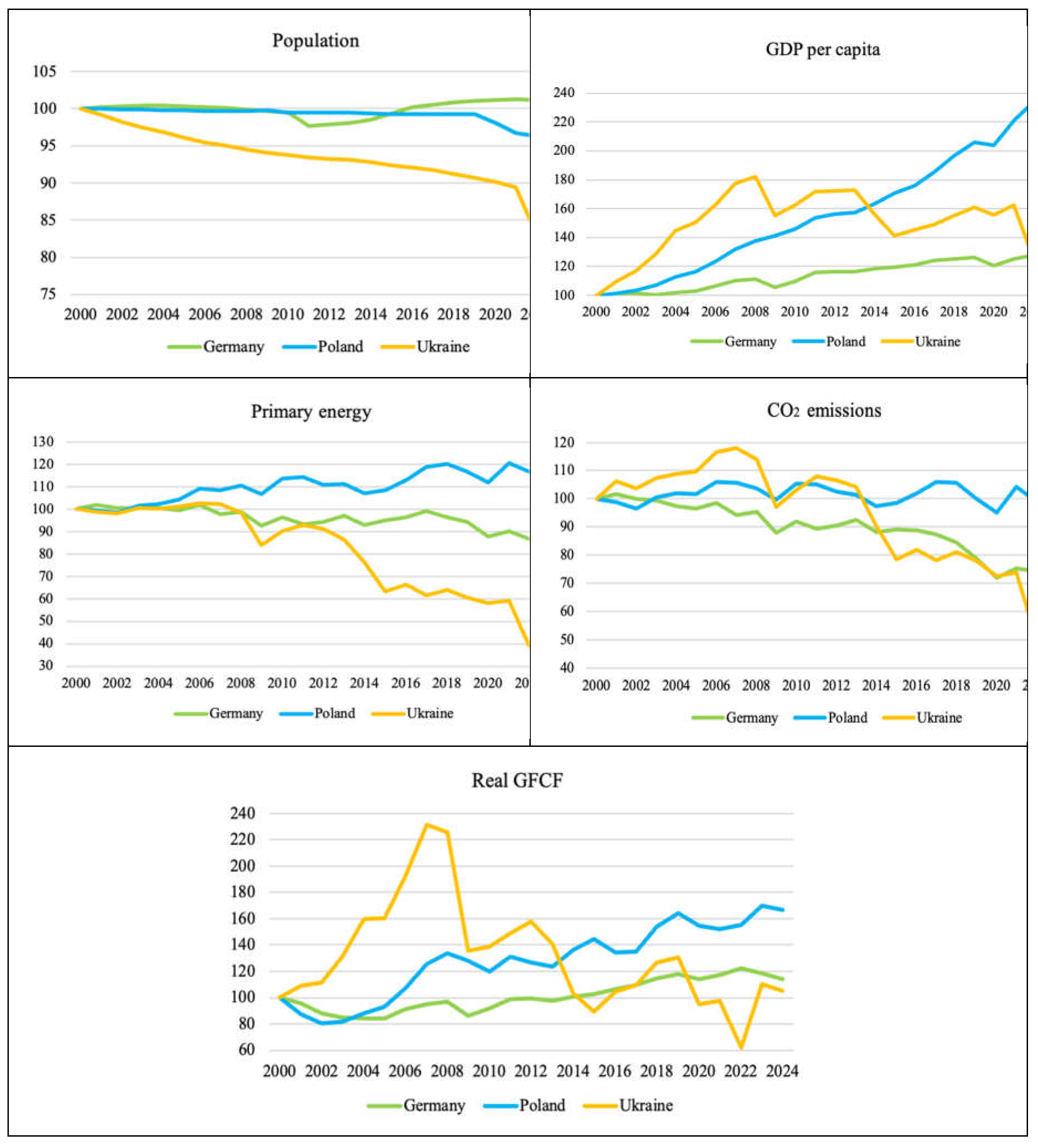
Figure 2.
Long-term LMDI decomposition of CO2 emissions change in Germany, Poland, and Ukraine, 1990-2024. Source: authors’ calculations.
Figure 2.
Long-term LMDI decomposition of CO2 emissions change in Germany, Poland, and Ukraine, 1990-2024. Source: authors’ calculations.
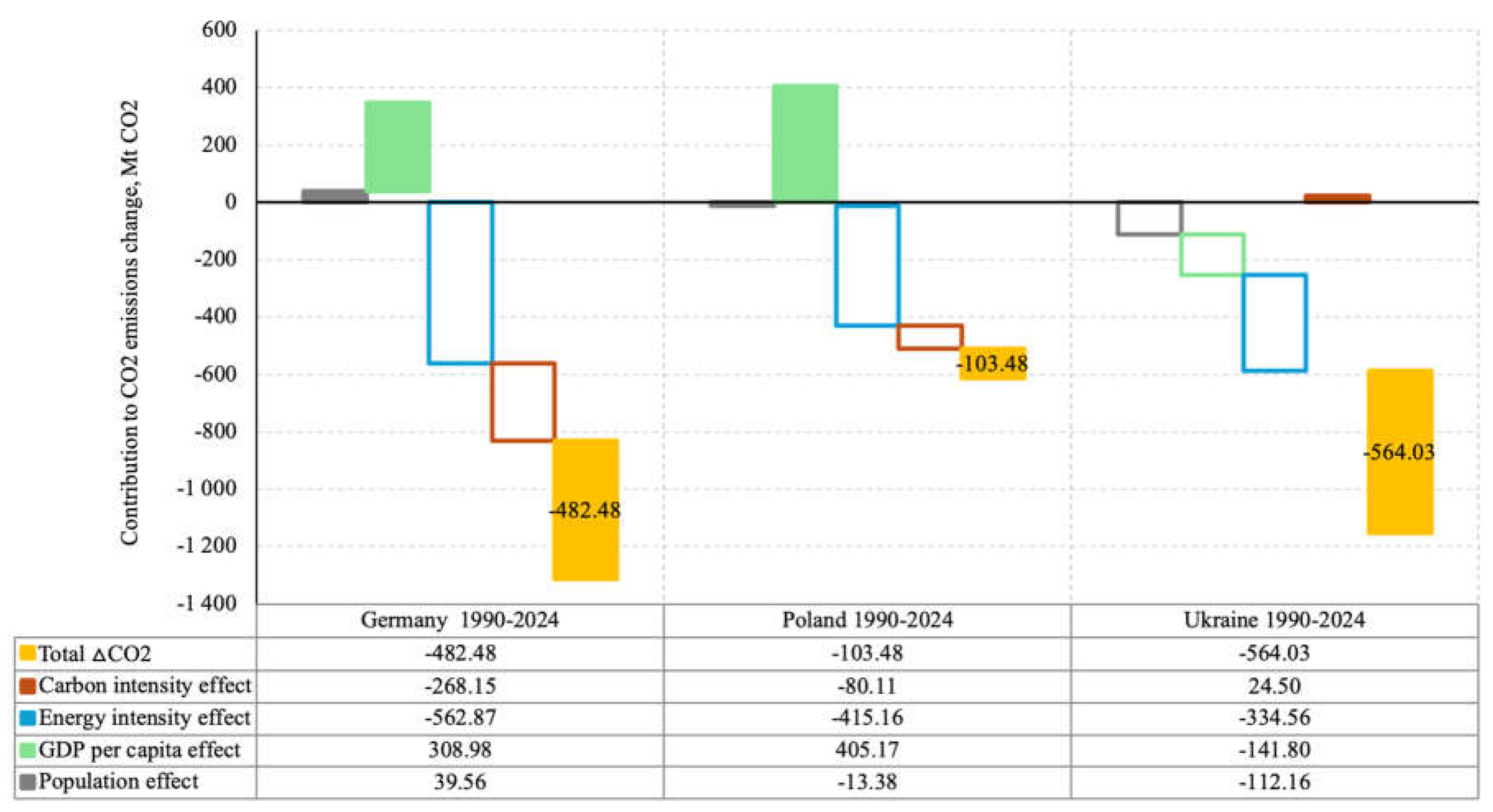
Figure 3.
LMDI decomposition of transformation and pre-2014 trajectories, 1990-2000 and 2000-2013. Source: authors’ calculations.
Figure 3.
LMDI decomposition of transformation and pre-2014 trajectories, 1990-2000 and 2000-2013. Source: authors’ calculations.
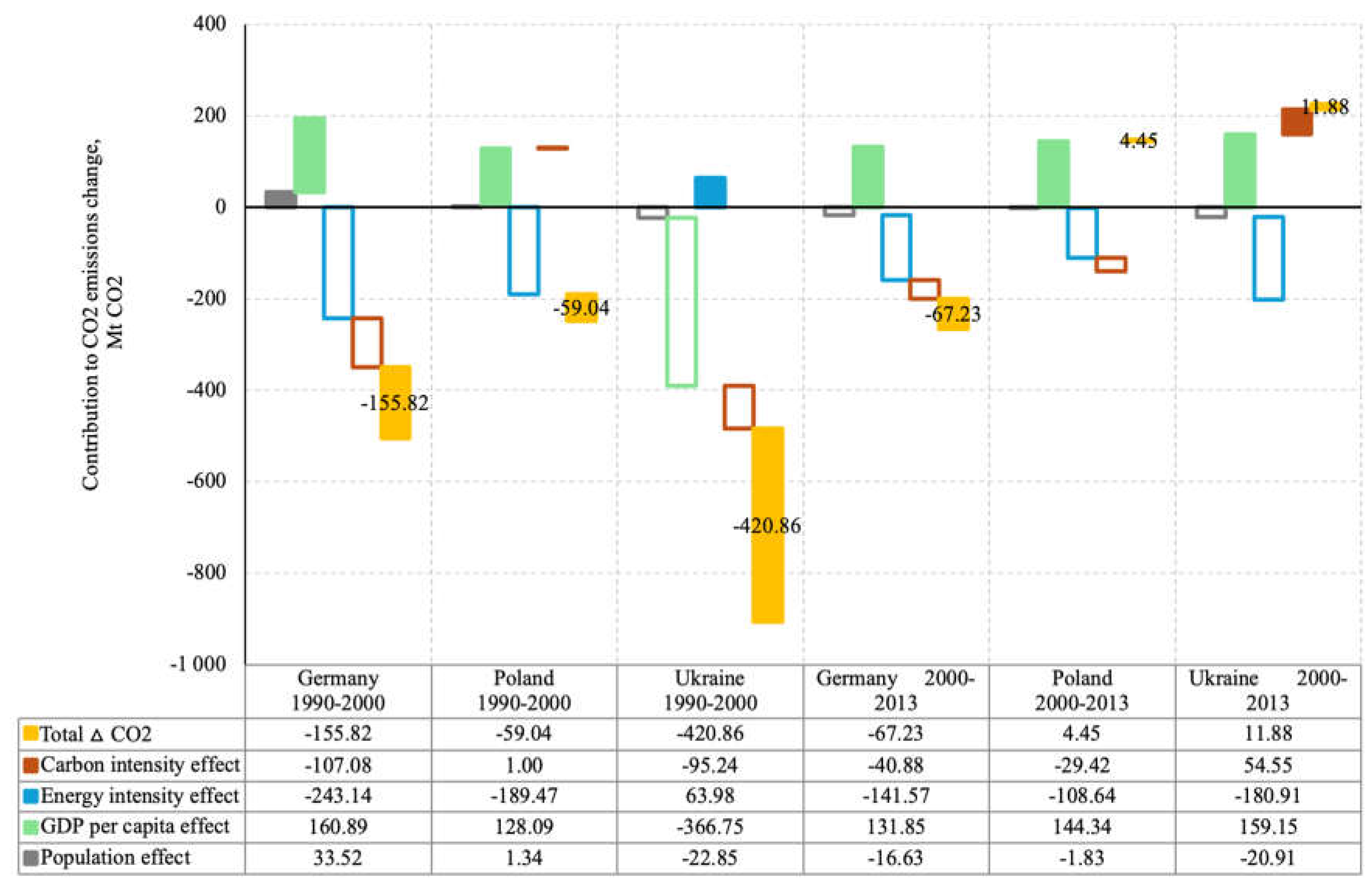
Figure 4.
LMDI decomposition of shock and adjustment periods, 2013-2024. Source: authors’ calculations.
Figure 4.
LMDI decomposition of shock and adjustment periods, 2013-2024. Source: authors’ calculations.
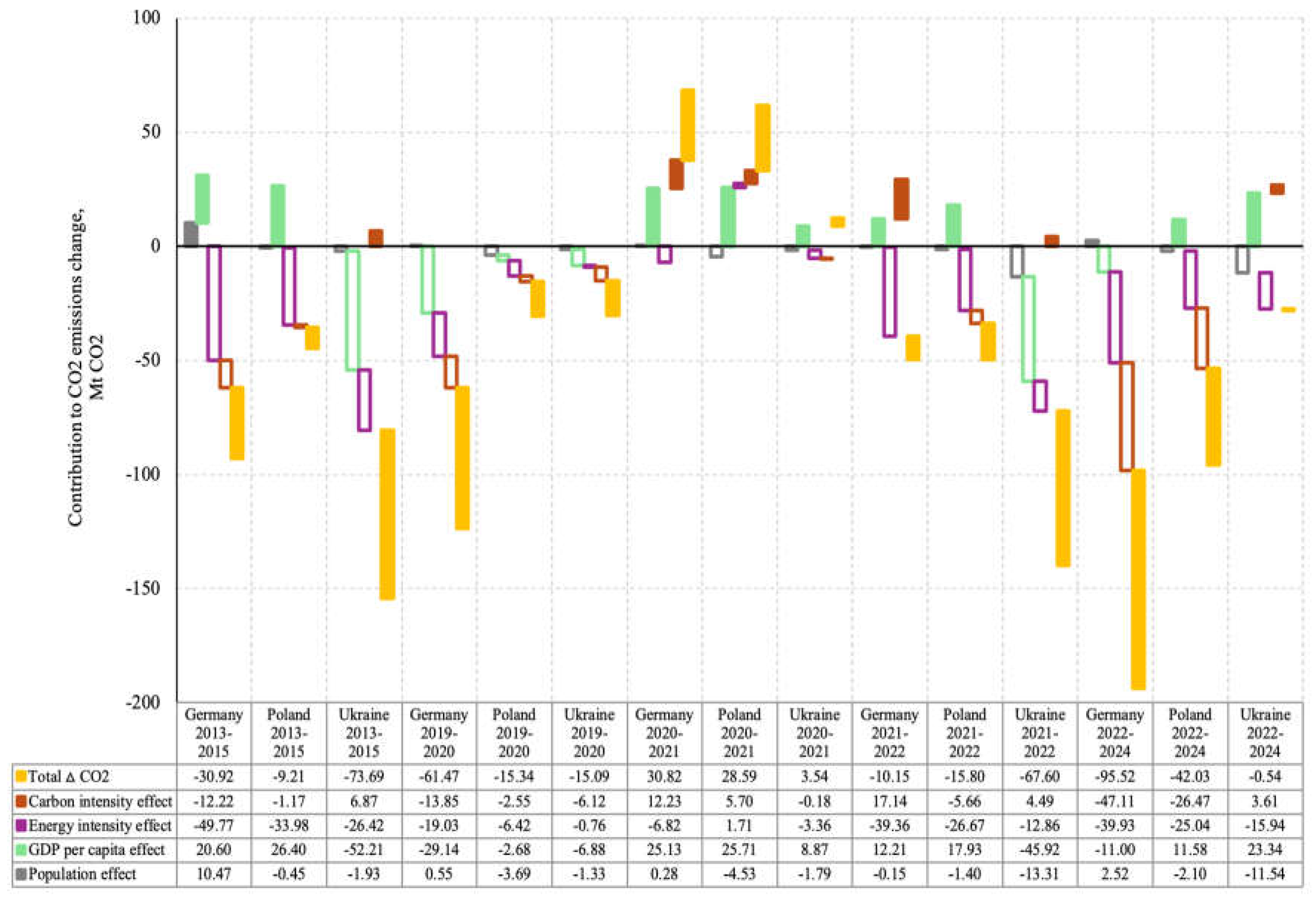
Figure 5.
Average gross fixed capital formation per tonne of CO2 by country and period, in constant 2021 international dollars. Source: authors’ calculations.
Figure 5.
Average gross fixed capital formation per tonne of CO2 by country and period, in constant 2021 international dollars. Source: authors’ calculations.
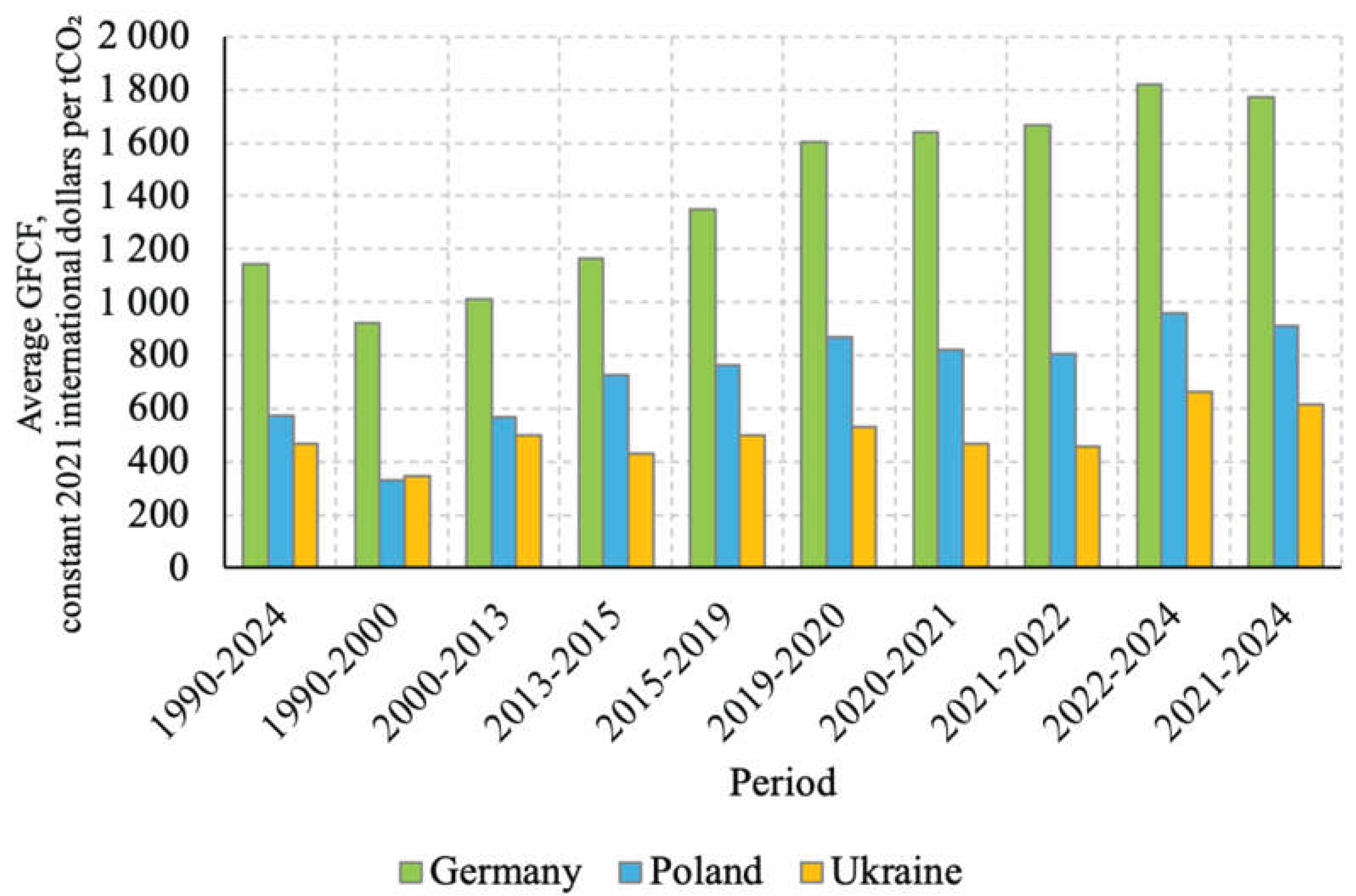
Table 2.
Major structural transformations and external shocks used to guide analytical periodization.
Table 2.
Major structural transformations and external shocks used to guide analytical periodization.
| Period | Germany | Poland | Ukraine |
| 1990-2000 | German reunification and restructuring of eastern Germany | Post-socialist transformation | Post-Soviet transformation shock |
| 2000-2013 | Economic growth and lower aggregate energy intensity | EU integration and modernization | Post-transformation recovery before 2014 |
| 2013-2015 | Continued transition and lower aggregate energy intensity | Continued EU integration | Occupation of Crimea and parts of Donbas; loss of industrial capacity |
| 2019-2020 | COVID-19 shock | COVID-19 shock | COVID-19 shock |
| 2020-2021 | Post-COVID recovery | Post-COVID recovery | Post-COVID recovery |
| 2021-2022 | Post-COVID recovery and energy crisis | Post-COVID recovery and energy crisis | Shock of Russia’s full-scale invasion |
| 2022-2024 | Energy-market adjustment | Energy-market adjustment | Wartime adaptation |
The periodization is interpretive and is used to prevent crisis-related emissions declines from being classified automatically as managed decarbonization.
Table 3.
Variables, units, sources, and analytical roles.
| Variable | Unit | Primary source | Use |
| Population | Persons | World Development Indicators [38,39] | Population effect in LMDI |
| GDP | Constant 2021 international dollars, Purchasing Power Parity (PPP) | World Development Indicators [38,40] | GDP per capita and activity effect |
| Primary energy | Energy units converted consistently across countries and years | Our World in Data/Energy Institute series [41,42,43] | Energy intensity and carbon intensity |
| CO2 emissions | Mt CO2, territorial fossil-fuel and industry emissions | Global Carbon Budget/Our World in Data [44,45] | Dependent accounting identity and denominator of IC |
| Gross fixed capital formation | Constant 2021 international dollars | World Development Indicators and authors’ harmonization [38,40,46] Data gaps in the World Bank series were filled by the authors based on [47,48,49] |
Investment-capacity proxy |
| Sector emissions intensity | tCO2/t steel; tCO2/t clinker; tCO2/MWh | Technical and industry sources [33,50,51,52,53] | Indicative gross carbon-cost exposure |
| Carbon prices | EUR/tCO2 | European Commission, ICAP, and World Bank [21,22,23,24] | Domestic and EU ETS/CBAM-equivalent scenarios |
Table 4.
Indicative gross carbon-cost exposure before free allocation, compensation, and pass-through at the principal benchmark.
Table 4.
Indicative gross carbon-cost exposure before free allocation, compensation, and pass-through at the principal benchmark.
| Country | Price signal | Steel (EUR/t) | Clinker (EUR/t) | Electricity (EUR/MWh) | Diagnostic interpretation |
| Germany | EU ETS / CBAM-equivalent | 131.7 | 59.5 | 25.7 | Material indicative gross industrial exposure; stronger reported investment-capacity indicators are consistent with comparatively greater capacity to finance modernization. |
| Poland | EU ETS/ CBAM-equivalent | 120.4 | 58.2 | 42.6 | The highest electricity exposure among the three cases reflects the carbon-intensive power mix and raises indirect pressure on industry. |
| Ukraine | Domestic carbon tax | 1.4 | 0.5 | 0.2 | The domestic signal is very weak and, on its own, provides only a limited carbon-price incentive for capital-intensive modernization. |
| Ukraine | EU ETS/ CBAM-equivalent | 181.4 | 65.1 | 23.8 | Indicative gross external exposure is more than 127 times the domestic-tax value; the steel and clinker results identify conditions consistent with elevated risk. |
The figures represent gross route- or sector-level exposure before free allocation, compensation, pass-through, and other firm-specific adjustments.
Table 7.
Integrated diagnostic interpretation of the three emissions trajectories.
| Country | Historical mechanism | Carbon-price condition | Investment capacity | Overall interpretation |
| Germany | Decline dominated by lower energy and carbon intensity despite higher GDP per capita | Strong, predictable, and institutionally embedded | Relatively high | Closest to managed decarbonization; hard-to-abate sectors remain exposed. |
| Poland | Energy-intensity-led decoupling; carbon-intensity improvement is more limited | Strong EU ETS signal; high power-sector exposure | Intermediate | Carbon-intensive decoupling; power-system transformation and just-transition investment are key priorities for a deeper transition. |
| Ukraine | Large decline shaped by transformation, population loss, lower activity, and war; long-term carbon-intensity effect is positive | Weak domestic signal; much stronger external CBAM-linked pressure | Low and disrupted | Structural/shock-driven decline; conditions are consistent with elevated contraction risk under future exposure when finance and technology options remain limited. |
Disclaimer/Publisher’s Note: The statements, opinions and data contained in all publications are solely those of the individual author(s) and contributor(s) and not of MDPI and/or the editor(s). MDPI and/or the editor(s) disclaim responsibility for any injury to people or property resulting from any ideas, methods, instructions or products referred to in the content. |
© 2026 by the authors. Licensee MDPI, Basel, Switzerland. This article is an open access article distributed under the terms and conditions of the Creative Commons Attribution (CC BY) license (http://creativecommons.org/licenses/by/4.0/).
Copyright: This open access article is published under a Creative Commons CC BY 4.0 license, which permit the free download, distribution, and reuse, provided that the author and preprint are cited in any reuse.