

Submitted:
27 August 2026
Posted:
31 August 2026
You are already at the latest version
Abstract
Electrically excited eddy current brakes (ECBs) with solid active material suffer from low power density due to non-uniform heat dissipation caused by the skin effect. This paper presents an anisotropic material structure consisting of flux-conducting steel pins surrounded by electrically conductive perforated sheets, which simultaneously reduces the skin effect and enables direct liquid cooling of the active material. Two structural variants are investigated: a PIN structure with cylindrical flux-conducting elements and a Cluster structure with elements in hexagonal cluster configuration. A computationally efficient 2D reluctance network model is developed for both variants, combining analytically derived reluctances with FEM pre-computed reluctances for air spaces and frequency-dependent reluctances of the flux-conducting elements. The model is validated against measured torque characteristics of two experimental demonstrators over the full range of excitation currents from 10 to 80 A. Good agreement between simulation and measurement is achieved after correcting for two systematic deviations identified during validation: a geometric effect at the inner and outer edges of the perforated sheets that reduces the effective eddy current path resistance, and the temperature dependence of the sheet resistance. The critical rotational speed is accurately reproduced by the corrected model. The uncertainty range due to undetermined thermal operating conditions is quantified, providing a reliable basis for the design and optimization of ECBs with anisotropic material structure.
Keywords:
eddy current brake
; reluctance model
; anisotropic material structure
1. Introduction
In electric vehicle applications, a wear-free eddy current brake (ECB) offers an attractive supplement to the friction brake. However, electrically excited ECBs with solid active material [1,2,3,4] suffer from low power density, limited to approximately 4 kW/kg [5], primarily due to non-uniform heat dissipation caused by the skin effect [6]. As shown in Figure 1a, the skin effect arises because eddy currents in a homogeneous, isotropic conductive material are coupled via a high-permeability magnetic circuit, allowing them to displace the primary field toward the surface.
To reduce the skin effect, the magnetic circuit must be interrupted in one direction, forcing the field to fully penetrate the material (Figure 1b). Since the relative permeability of real materials cannot drop significantly below , the skin effect cannot be completely eliminated, but only reduced.
Even with anisotropic materials, the relative permeability in the direction of low magnetization still reaches at [7,8], so a macroscopically anisotropic structure is required. This is realized by flux-conducting steel pins surrounded by electrically conductive perforated sheets [9], as shown in Figure 2a. The gaps between the stacked sheets simultaneously serve as cooling channels, significantly increasing the free surface area in contact with the cooling medium. The torque characteristic can be tailored via the geometric parameters of the structure.
To further reduce the skin effect within the cylindrical pins, multiple thin pins can be grouped in a hexagonal cluster configuration (Figure 2b) [10]. These two variants the PIN structure and the Cluster structure are the subject of this work.
Figure 3 shows a functional illustration of a rotating ECB with the anisotropic material structure. This paper presents a 2D reluctance-network-based electromagnetic model for both structure variants and validates it experimentally against measured torque characteristics.
The material structure with cylindrical flux-conducting elements is hereinafter referred to as the PIN structure, while the material structure with flux-conducting elements in a hexagonal cluster configuration is designated the Cluster structure. Figure 3 shows an exemplary CAD design of a rotating eddy current brake with the described anisotropic material structure as a Pin structure. In this work the electromagnetic model of the proposed eddy current brake with anisotropic material structure is presented and validated in detail.
2. Electromagnetic Model
The electromagnetic model calculates the mean torque over one revolution for a given excitation current and rotational speed n. A full 3D FEM simulation of the ECB with anisotropic material structure is computationally prohibitive for design optimization. Due to the skin effect, a fine mesh is required at the pin surfaces, resulting in a mesh with a large number of elements at maximum speed. Combined with the 3000 time steps required to reach a quasi-steady state, the computation time for a single operating point exceeds several hundred hours on modern hardware [2]. A reluctance network model, by contrast, abstracts the electromagnetic domain into flux tubes, each characterized by a reluctance determined analytically or by FEM pre-computation. The resulting system of equations is small and computationally efficient, yet sufficiently accurate for torque prediction [11,12]. A hybrid approach is adopted here, in which air-space reluctances with non-uniform flux density are pre-computed by FEM [13,14]
The following simplifications are adopted: (i) the ECB is represented by a 2D reluctance model in a representative plane; (ii) flux-conducting elements form flux tubes with analytically derived reluctances; (iii) torque ripple is negligibly small. Reluctances of regions with non-uniform flux density are pre-computed by FEM. The mean torque follows from the energy balance:
where is the mean eddy-current Joule heat, the mean iron losses, and the ventilation losses (assumed negligible).
2.1. Representative Mapping of the Geometry in 2D
In axial-flux machines such as the ECB, the pole pitch varies with radius, so a representative model plane must be chosen. Assuming the torque-generating force originates equally from the inner and outer surfaces, the model diameter satisfies:
With the number of pole pairs the model pole pitch is . To exploit anti-periodic boundary conditions, the number of flux-conducting elements per model pole pitch is rounded to the nearest integer, giving a representative element spacing and a representative element diameter that preserves the real fill factor of the flux conducting elements . The real and model arrangements are illustrated in Figure 4.
2.2. Reluctance Network Model
Applying Hopkinson’s law [12] and Ampere’s circuital law to each mesh m of N reluctances, the governing equation of a mesh-flux reluctance network is:
where is the mesh flux of mesh m, the adjacent mesh flux, and the mesh current. Figure 5 shows the reluctance model for one pole using antisymmetric boundary conditions. The model depth equals . The excitation part consists of a yoke with pole cores surrounded by excitation coils. The magnetic flux traverses the air gap (reluctance ) and the flux-conducting elements (). Tangential leakage between adjacent elements is accounted for by . Eddy currents are induced by the time-varying fluxes, where indices i and j denote the tangential and axial position respectively.
Applying (3) to each material-structure mesh and using Faraday’s law, the eddy current is:
where the time derivative is approximated by a central difference at constant tangential velocity . The governing equation to be solved is:
For the meshes assigned to the air gap and the excitation circuit, the general equation (3) applies with the excitation current . The resulting system of equations is solved iteratively using the biconjugate gradient method [15], accounting for the nonlinear magnetization curves of the respective materials.
The total Joule heating power resulting from the eddy currents in meshes can be calculated using equation (4) and the mesh fluxes determined by solving equation (5), via
The second summation term accounts for the fact that this is a half-model, and that for an odd total number of perforated sheets j, the Joule losses of the last sheet are counted at half weight. Note that the floor brackets in the upper limit of the sum over all j in the first term and the ceiling brackets at the index in the second term must be observed. The path resistances of the eddy currents between the flux-conducting elements are described in subSection 2.4.
2.3. Modeling of the Reluctances
For a homogeneous flux density distribution and constant cross-sectional area, a reluctance is obtained from the length of a flux path , its cross-sectional area , and the permeability of the material .
An approximately homogeneous flux density is present in the yoke and the pole core of the exciter. The relative permeability of all ferromagnetic components is determined iteratively from the measured magnetization curve of the respective material, which is extended using the saturation model from [16]. For all air-space reluctances — including the air gap and tangential leakage between flux-conducting elements — a scalar magnetic potential FEM model is used. In current-free regions, the scalar magnetic potential satisfies the Laplace equation , which is solved numerically with prescribed potential boundary conditions and . The reluctance follows directly from the resulting magnetic flux as . To calculate the air gap reluctance, it is convenient to multiply the air gap reluctance obtained by neglecting leakage fluxes by a factor, referred to here as , which accounts for the leakage flux.
Due to the linear behavior of the air region, the factor depends only on geometric ratios. This factor is evaluated after a FEM simulation as follows.
Due to the linear behavior of the air region, the factor depends only on geometric ratios. This factor is evaluated after a FEM simulation as follows:
Figure 6a and Figure 6b illustrate the computational domain used to determine the air gap reluctance above the flux-conducting elements. The corresponding results are presented in Figure 6. Figure 6c and Figure 6d show the magnetic flux density vectors obtained from the FEM calculations. The resulting reluctance factor is plotted as a function of the ratio of air gap to pin diameter for various fill factors, for the PIN structure in Figure 7a and for the Cluster structure in Figure 7b. The reluctances of the flux-conducting elements them self’s are frequency- and field-strength-dependent due to the skin effect, and are pre-computed via a harmonic 2D FEM model [17].
2.4. Modeling of the Path Resistance
Due to the perforations in the conductive sheets, the resistance of the eddy current path depends on the opening ratio of the perforated sheets. Furthermore, in the 2D model the return path of the eddy currents at the inner and outer sides is neglected. The resistance at the inner and outer sides can be accounted for by the so-called Russell-Norsworthy factor [18]. The dependence of the effective conductivity on the fill factor of the flux-conducting elements is calculated using a FEM model of a partial segment of the eddy current path. Since the relationship between current density and electric field strength is linear, a resistance factor is determined as a function of the fill factor. This factor indicates the ratio of the resistance of a path with perforations to a path without perforations. The resistance of a non-perforated path of width , length , thickness s, and specific resistance is given by:
Using the FE models in Figure 8, the current through the path segment and thus the resistance can be determined for given potential boundary conditions and via
From the FEM calculation, the resistance factor can be evaluated as
Figure 8c shows the resistance factor as a function of the opening ratio of a perforated sheet with hexagonal perforations (red) and cylindrical perforations (blue).
The difference between the two variants at high opening ratios arises from the fact that for hexagonal perforations the resistance only tends to infinity as the opening ratio approaches 1, whereas for cylindrical perforations this already occurs at an opening ratio of . Using the resistance factor determined in this way, the resistance of the eddy current path between two flux-conducting elements of a perforated sheet with index j can be determined via
Since in the reluctance model the reference path width and the reference path length correspond to the spacing of the flux-conducting elements, the reference resistance, accounting for the temperature of the perforated sheet j with the specific resistance at and the temperature coefficient , is:
It should be noted that not only the temperature may differ across all j, but also the material properties and .
3. Experimental Investigation and Model Validation
The primary objective of the investigation is the measurement of the torque characteristics of the demonstrator using various derivatives of the stator as a function of the excitation current. The derivatives differ in particular in their size, the type of magnetically conductive elements (cylindrical or hexagonal), and the number of perforated sheets within the material structure. Figure 9a shows a stator with cylindrical flux-conducting elements (PIN structure) and Figure 9b shows a stator with flux-conducting elements in hexagonal cluster configuration (Cluster structure).
The torque is measured as a function of rotational speed at excitation currents of – in increments of . Figure 10 shows the calculated torque characteristics compared to the measured ones at various excitation currents for the ECB with pin-structure Figure 10a and for the ecb with cluster-structure Figure 10b.
For validation purposes, in addition to the excitation current, the measured air gap is incorporated into the electromagnetic model. Nevertheless, deviations can be observed that can be attributed to identifiable sources of error, as described in the following subsection “Identification of Error Sources and Error Correction”.
3.0.1. Identification of Error Sources and Error Correction
As a first step in the error analysis, it is useful to calculate the torque characteristics from measured magnetic fluxes in the flux conducting elements. This allows errors of the reluctance network to be separated from errors due to incorrect resistances of the eddy current paths. The flux probes are positioned in the material-structure as shown in the picture in Figure 11. The flux density’s measured via field coil 1 and field coil 3 are shown in Figure 11 with the solid lines at an excitation current of and a rotational speed of .
The mesh fluxes in equation 4 can be replaced by the measured fluxes in the flux-conducting elements , since
Thus, equation 4 can be written as:
. It then follows for equation 6 that
The magnetic fluxes are determined by interpolating the measured fluxes at positions i of the flux-conducting elements beneath a pole. In the axial direction (depth direction) with index j, the magnetic fluxes are determined under the assumption that the magnetic flux decays exponentially. The measured fluxes and interpolated at position i (markers directly on the lines in Figure 11) are used to calculate an exponential coefficient with
in order to determine the magnetic fluxes (markers in Figure 11) with
for equation 18.
The torque is finally determined via equation 1. Figure 12 shows the directly measured torque characteristics (markers) and the torque characteristics calculated from the measured magnetic fluxes at , , and with solid lines. It can be seen that the torque characteristic calculated from the measured magnetic fluxes at agrees very well with the directly measured one. However, at excitation currents of and , a significant deviation can be observed. Since this deviation is more pronounced at than at , it can be assumed that the deviation is a consequence of heating of the perforated sheets, which is more pronounced at higher power levels.
According to this hypothesis, this error can potentially be corrected by accounting for the temperature dependence of the specific resistance of the perforated sheets. In the correction calculation, the measured temperature of the perforated sheets is therefore incorporated into the calculation of the eddy current path resistances.
Furthermore, it is clearly visible in Figure 10b that the critical rotational speed of the calculated torque characteristics is significantly higher than that of the measured ones, even at low excitation currents. This can be attributed to the fact that the resistance of the current paths of the perforated sheets in the experimental demonstrator is lower than assumed in the model. The reason for this becomes apparent in Figure 13b, which shows the FEM models used to analyze the error. In the model, it is assumed that the current paths at the edge of the perforated sheets have the same cross-section as between the flux-conducting elements in the center, as shown in Figure 13b.
In the real design, however, potential perforations that would extend beyond the outer diameter are not realized. As a result, the current path at the edge is on average significantly wider, leading to a lower resistance of the eddy current paths, as shown in Figure 13a. This circumstance ultimately leads to a reduction of the Russell-Norsworthy factor, which, as described in Section 2.4, accounts for the resistance that the eddy currents must overcome at the edges.
The correction factor for this reduction is determined using the FEM models shown in Figure 13. In the FEM models with periodic boundary conditions of a 60-degree segment, each flux-conducting element at position i in the polar coordinate system is assigned a flux change , which describes a cosine function in the tangential direction with angle , amplitude , and periodicity of the pole pair number p.
The plane of symmetry corresponds to an angle of zero. Since the FEM software used allows only a limited number of voltage sources as boundary conditions, a 60-degree segment is simulated and a pole pair number of 6 is chosen in order to exploit the periodic boundary conditions. The resulting current density at the edges and in the center of the computational domain is evaluated as a result. Figure 14 shows the current density in the normal direction along the evaluation paths (edge and center) corresponding to Figure 13a (real perforated sheet) with blue lines and with red lines for the evaluation paths in Figure 13b (perforated sheet corresponding to the model). The correction value for the Russell-Norsworthy factor can be determined by taking the ratio of the total currents along the evaluation paths of the model sheet to the total currents of the real sheet . Since the integral of the positive current density must equal the integral of the negative current density along an evaluation path, the total current is determined via the integral of the absolute value of the current density, which is then halved. The correction factor for the Russell-Norsworthy factor is thus:
From the evaluation of equation 22, a correction value for the Russell-Norsworthy factor of is obtained. The mean resistance of the eddy current paths of the real perforated sheets is therefore 15% lower than assumed in the model.
The solid lines in Figure 12 show the torque characteristics calculated from the measured magnetic fluxes, accounting for the measured temperature of the perforated sheets (indicated by the colored markers) and the correction value of the Russell-Norsworthy factor. The outliers at and in the range from to are attributable to errors in the measurement of the magnetic flux. Figure 15 illustrates, using the torque characteristic at an excitation current of , the separate influence of the correction of the Russell-Norsworthy factor and the correction of the resistance through the temperature effect of the perforated sheets. Neglecting the temperature effect leads to a lower torque above the critical rotational speed, while neglecting the correction of the Russell-Norsworthy factor results in a shift of the calculated torque characteristic toward higher rotational speeds.
The uncertainty range due to undetermined thermal parameters is determined in subSection 3.1.
3.1. Determination of the Uncertainty Range of the Overall Models due to Undetermined Thermal Parameters
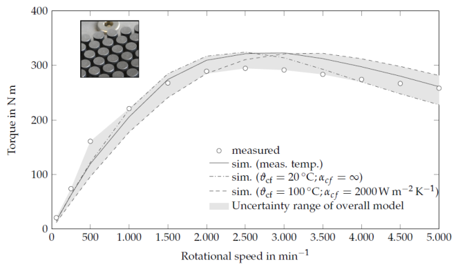
Since the model validation is carried out accounting for the measured temperature, the uncertainty range is investigated here on the basis of the coolant inlet temperature and the heat transfer coefficient to the coolant.
In the following analysis, the torque characteristic at an excitation current of is calculated for various combinations of undetermined thermal parameters. A distinction is made between a high coolant temperature of in combination with a low heat transfer coefficient for forced convection of [19], and a coolant temperature of in combination with an infinitely high heat transfer coefficient.
For this analysis, the overall model is extended with a simplified thermal model of the material structure. In each iteration step for solving the nonlinear reluctance network, the temperature of the perforated sheets is calculated based on the inlet temperature, the heat transfer coefficient, and the current Joule heat of the respective perforated sheet, along with the resulting electrical conductivity, which feeds into equation in the next iteration step.
Figure 16 and Figure 17 show the simulated torque characteristics accounting for the bounds of the coolant temperature and heat transfer for the ECB with Cluster structure (Figure 16) and for the ECB with PIN structure (Figure 17).
At a coolant temperature of and a heat transfer coefficient of , the torque characteristic is slightly compressed along the rotational speed axis compared to the simulation accounting for the measured temperature, while at a coolant temperature of and a heat transfer coefficient of , the torque characteristic is stretched along the rotational speed axis. The resulting uncertainty range is indicated by the shaded area. Since the coolant inlet temperature can vary during operation, this uncertainty range must be taken into account in future design work.
4. Conclusion
This paper presents a computationally efficient 2D reluctance network model for electrically excited eddy current brakes with anisotropic material structure, covering both the PIN structure with cylindrical flux-conducting elements and the Cluster structure with flux-conducting elements in hexagonal cluster configuration. The model accounts for the nonlinear magnetization behavior of the flux-conducting elements, the frequency- and field-strength-dependent reluctances determined by FEM, and the temperature-dependent path resistance of the perforated sheets. Experimental validation against measured torque characteristics of two demonstrators shows good agreement between simulation and measurement after applying two corrections: a correction of the Russell-Norsworthy factor to account for the geometry of the real perforated sheets at the inner and outer edges ( for the Cluster structure, for the PIN structure), and a temperature correction based on the measured sheet temperatures. In particular, the critical rotational speed is accurately reproduced by the corrected model. Residual deviations of up to 15% at high excitation currents and low speeds are attributed to uncertainties in the magnetization curve of the flux-conducting elements. The uncertainty range of the overall model due to undetermined thermal parameters, namely the coolant inlet temperature and the heat transfer coefficient, was quantified and must be considered in future design applications. The model provides a suitable basis for the design and optimization of eddy current brakes with anisotropic material structure.
Author Contributions
Conceptualization, methodology, validation, C.H. and C.K.; formal analysis, A.M.. All authors have read and agreed to the published version of the manuscript.
Conflicts of Interest
Declare conflicts of interest or state “The authors declare no conflicts of interest.”.
Abbreviations
The following abbreviations are used in this manuscript:
| ECB | eddy current brake |
| FEM | finite element method |
References
- Ren, Q.; Zhang, J.; Luo, J. Characteristic Analysis and Control of a Rotary Electromagnetic Eddy Current Brake. Appl. Comput. Electromagn. Soc. 2021, 36, 806–815. [Google Scholar] [CrossRef]
- Ye, L.; Yang, G.; Li, D. Analytical model and finite element computation of braking torque in electromagnetic retarder. Front. Mech. Eng. 2014, 9, 368–379. [Google Scholar] [CrossRef]
- Zhang, B.; Peng, T.; Chen, Q.; Cao, Q.L.; Ji, K.; Shuang, B.; Ye, J.J.; Li, L. 3-D nonlinear transient analysis and design of eddy current brake for high-speed trains. Int. J. Appl. Electromagn. Mech. 2012, 40, 205–214. [Google Scholar] [CrossRef]
- Yaojing, F.; Xiangshuai, X.; Shoudao, H. Design research of high power oil-cooled electrical eddy current retarder for heavy vehicles. In Proceedings of the 2016 19th International Conference on Electrical Machines and Systems (ICEMS), 2016; pp. 1–5. [Google Scholar]
- Holtmann, C.; Rinderknecht, F.; Mockel, A. Analysis of the Thermal Limits of Conventional Eddy Current Brakes based on a Thermal 1d-Model. In Proceedings of the 2022 Second International Conference on Sustainable Mobility Applications, Renewables and Technology (SMART); IEEE, 2022; pp. 1–8. [Google Scholar] [CrossRef]
- Wheeler, H.A. Formulas for the Skin Effect. Proc. IRE 1942, 30, 412–424. [Google Scholar] [CrossRef]
- Müller, F.; Bavendiek, G.; Leuning, N.; Schauerte, B.; Hameyer, K. Consideration of ferromagnetic anisotropy in electrical machines built of segmented silicon steel sheets. IET Sci. Meas. Technol. 2020, 14, 242–249. [Google Scholar] [CrossRef]
- Shirkoohi, G.H.; Arikat, M. Anisotropic properties of high permeability grain-oriented 3.25% Si-Fe electrical steel. IEEE Trans. Magn. 1994, 30, 928–930. [Google Scholar] [CrossRef]
- Christoph Holtmann. Elektrodynamische Bremse. DE102016108646B4, 10.05.2016. DE102016108646B4.
- Holtmann, C.; Köhler, C.; Weber, C. DE 10 2022 128 247 B3; Induktionseinrichtung, insbesondere für eine elektrodynamische Bremse, und elektrodynamische Bremse. 2022.
- Rasmussen, C.B.; Ritchie, E. A magnetic equivalent circuit approach for predicting PM motor performance. In Proceedings of the Conference record of the 1997 IEEE Industry Applications Conference - Thirty-Second IAS Annual Meeting, Piscataway, NJ, 1997; pp. 10–17. [Google Scholar] [CrossRef]
- Kallenbach, E.; Eick, R.; Quendt, P.; Ströhla, T.; Feindt, K.; Kallenbach, M. Elektromagnete: Grundlagen, Berechnung, Entwurf und Anwendung; mit 34 Tabellen, 3. In Studium; bearb. und erg. aufl. ed.; Vieweg + Teubner: Wiesbaden, 2008. [Google Scholar]
- Ramirez-Laboreo, E.; Sagues, C. Reluctance actuator characterization via FEM simulations and experimental tests. Mechatronics 2018, 56, 58–66. [Google Scholar] [CrossRef]
- Sanabria-Walter, C.; Polinder, H. Analytical-numerical hybrid model for flux-switching permanent magnet machines. In Proceedings of the IECON 2013, Piscataway, NJ, 2013; pp. 2614–2619. [Google Scholar] [CrossRef]
- van der Vorst, H.A. Bi-CGSTAB: A Fast and Smoothly Converging Variant of Bi-CG for the Solution of Nonsymmetric Linear Systems. SIAM J. Sci. Stat. Comput. 1992, 13, 631–644. [Google Scholar] [CrossRef]
- Bertenshaw, D.R.; Smith, A.C. Lamination joint reluctance in stator cores: a forgotten problem? In Proceedings of the 7th IET International Conference on Power Electronics, Machines and Drives (PEMD 2014), 2014; pp. 2.7.02–2.7.02. [Google Scholar] [CrossRef]
- Jack, A.G.; Mecrow, B.C. Methods for magnetically nonlinear problems involving significant hysteresis and eddy currents. IEEE Trans. Magn. 1990, 26, 424–429. [Google Scholar] [CrossRef]
- Edwards, J.D.; Jayawant, B.V.; Dawson, W.; Wright, D.T. Permanent-magnet linear eddy-current brake with a non-magnetic reaction plate. IEE Proc.-Electr. Power Appl. 1999, 146, 627. [Google Scholar] [CrossRef]
- Cerbe, G.; Hoffmann, H.J. Einführung in die Wärmelehre: Von d. Thermodynamik zur techn. Anwendung; mit 111 Beisp., 118 Aufgaben u. 161 Kontrollfragen, 7., neubearb. u. erw. aufl. ed.; Studienbücher der technischen Wissenschaften, Hanser: München, 1986.
Figure 1.
Visualization of the problem (a) and the proposed solution (b).
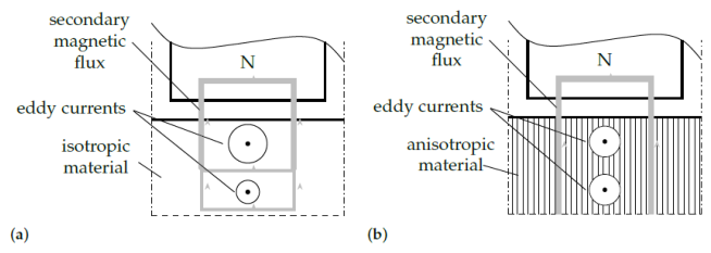
Figure 2.
Solution approach with cylindrical flux-conducting elements (a) and with flux-conducting elements in hexagonal cluster configuration (b).
Figure 2.
Solution approach with cylindrical flux-conducting elements (a) and with flux-conducting elements in hexagonal cluster configuration (b).
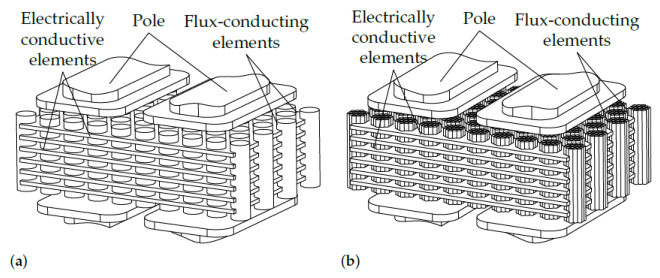
Figure 3.
Functional illustration of an eddy current brake with anisotropic material structur.
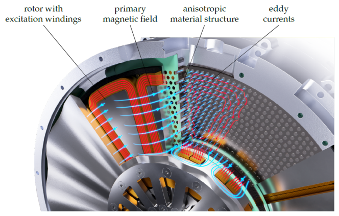
Figure 4.
Real arrangement of the flux-conducting elements (a) and arrangement of the flux-conducting elements in the model (b).
Figure 4.
Real arrangement of the flux-conducting elements (a) and arrangement of the flux-conducting elements in the model (b).
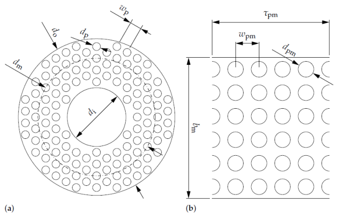
Figure 5.
Reluctance model with reluctances of ferromagnetic components shown in dark gray and reluctances of air spaces shown in white. Shown in light gray are reluctances resulting from the series combination of the air gap reluctances and the reluctance of the upper portions of the flux-conducting elements.
Figure 5.
Reluctance model with reluctances of ferromagnetic components shown in dark gray and reluctances of air spaces shown in white. Shown in light gray are reluctances resulting from the series combination of the air gap reluctances and the reluctance of the upper portions of the flux-conducting elements.
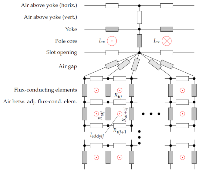
Figure 6.
Calculation of air gap reluctance over flux-conducting elements. (a) Computational domain geometry for cylindrical flux-conducting element (b) Computational domain geometry for hexagonal cluster flux-conducting element (c) Magnetic flux density vectors from FEM simulation of cylindrical flux-conducting element (d) Magnetic flux density vectors from FEM simulation of hexagonal cluster flux-conducting element.
Figure 6.
Calculation of air gap reluctance over flux-conducting elements. (a) Computational domain geometry for cylindrical flux-conducting element (b) Computational domain geometry for hexagonal cluster flux-conducting element (c) Magnetic flux density vectors from FEM simulation of cylindrical flux-conducting element (d) Magnetic flux density vectors from FEM simulation of hexagonal cluster flux-conducting element.
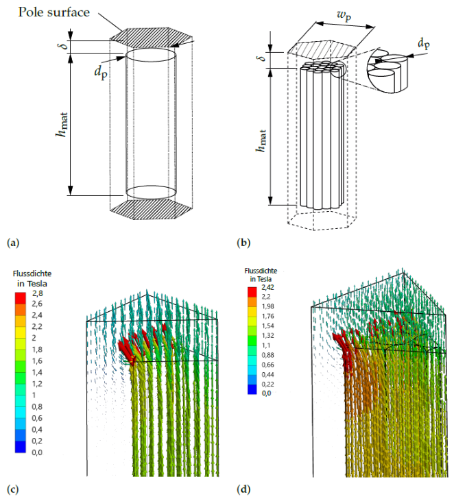
Figure 7.
Airgap reluctance factor as a function of the ration of the airgab and the pin diameter for different pin-filling factors as a result of the fem analyses for the pin-structure (a) and the cluster-structure (b).
Figure 7.
Airgap reluctance factor as a function of the ration of the airgab and the pin diameter for different pin-filling factors as a result of the fem analyses for the pin-structure (a) and the cluster-structure (b).
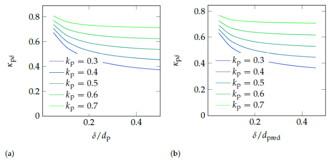
Figure 8.
FE models for calculating the resistance of a sheet segment with cylindrical perforations (a) and hexagonal perforations (b), and resistance factor as a function of the opening ratio as a result of the FEM calculation (c).
Figure 8.
FE models for calculating the resistance of a sheet segment with cylindrical perforations (a) and hexagonal perforations (b), and resistance factor as a function of the opening ratio as a result of the FEM calculation (c).
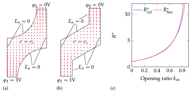
Figure 9.
Stator with cylindrical flux-conducting elements (PIN structure) (a) and with flux-conducting elements in hexagonal cluster configuration (Cluster structure) (b).
Figure 9.
Stator with cylindrical flux-conducting elements (PIN structure) (a) and with flux-conducting elements in hexagonal cluster configuration (Cluster structure) (b).
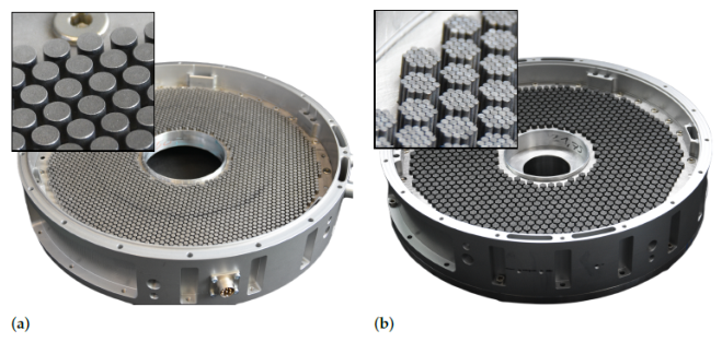
Figure 10.
Stator with cylindrical flux-conducting elements (PIN structure) (a) and with flux-conducting elements in hexagonal cluster configuration (Cluster structure) (b).
Figure 10.
Stator with cylindrical flux-conducting elements (PIN structure) (a) and with flux-conducting elements in hexagonal cluster configuration (Cluster structure) (b).
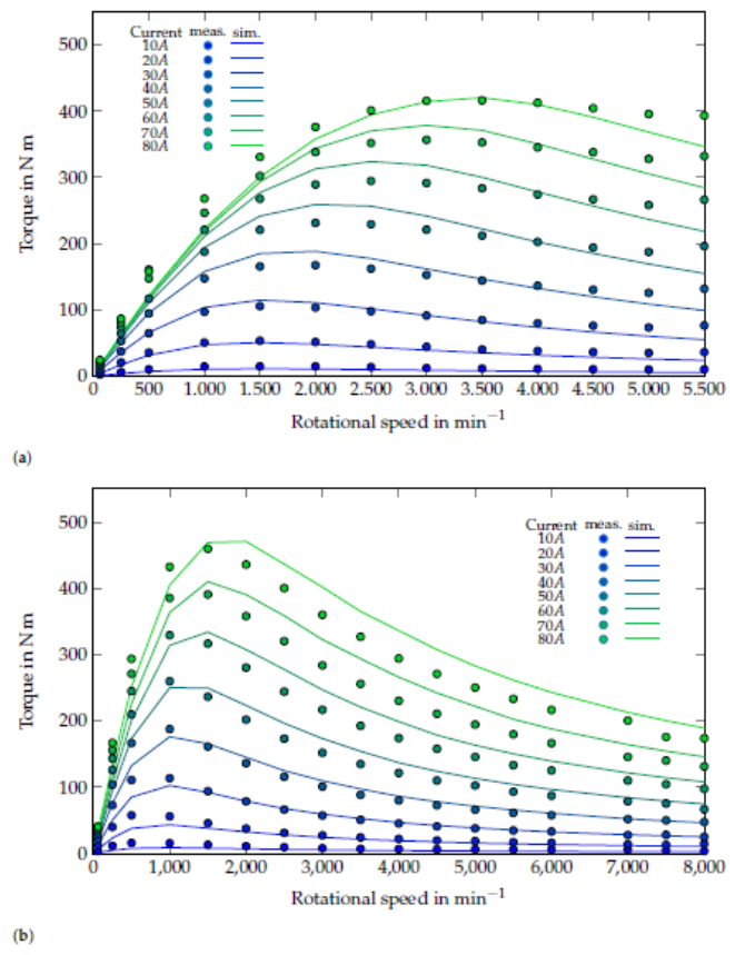
Figure 11.
Flux density measured via field coil 1 and field coil 3 at an excitation current of and a rotational speed of , and flux densities interpolated therefrom at the positions of the flux-conducting elements with index i and at the positions of the perforated sheets with index j.
Figure 11.
Flux density measured via field coil 1 and field coil 3 at an excitation current of and a rotational speed of , and flux densities interpolated therefrom at the positions of the flux-conducting elements with index i and at the positions of the perforated sheets with index j.
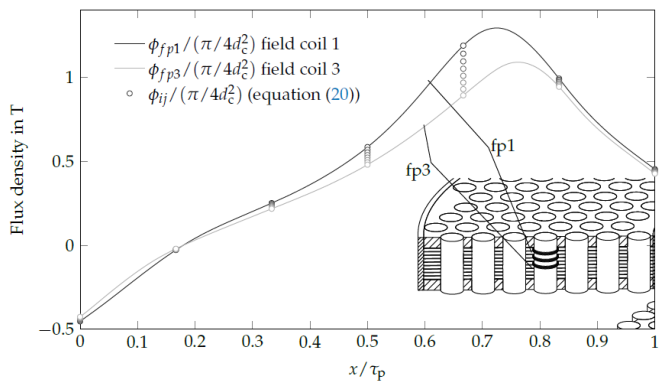
Figure 12.
Directly measured torque characteristics (markers) and torque characteristics calculated from the measured magnetic fluxes of the ECB with Cluster structure.
Figure 12.
Directly measured torque characteristics (markers) and torque characteristics calculated from the measured magnetic fluxes of the ECB with Cluster structure.
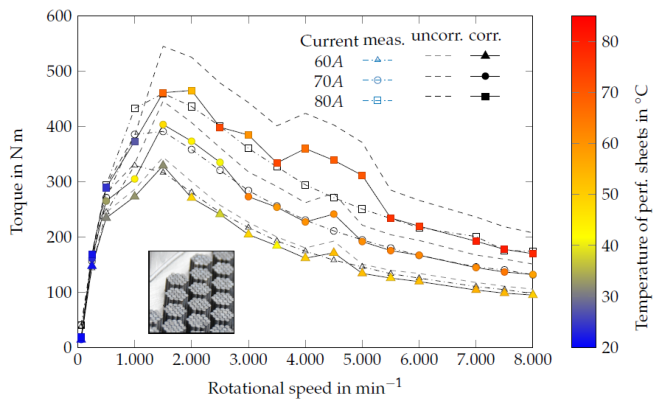
Figure 13.
FEM models (of the real sheet (A) and the model-equivalent sheet (B)) for determining the correction value for the Russell-Norsworthy factor. The current density normal to the evaluation paths is shown in Figure 14 with the corresponding lines.
Figure 13.
FEM models (of the real sheet (A) and the model-equivalent sheet (B)) for determining the correction value for the Russell-Norsworthy factor. The current density normal to the evaluation paths is shown in Figure 14 with the corresponding lines.
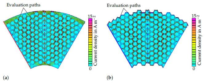
Figure 14.
Current density normal to the evaluation paths in Figure 13b (dashed) and current density normal to the evaluation path in Figure 13a (solid). Gray lines indicate the evaluation path at the edge and black lines the evaluation path at the center.
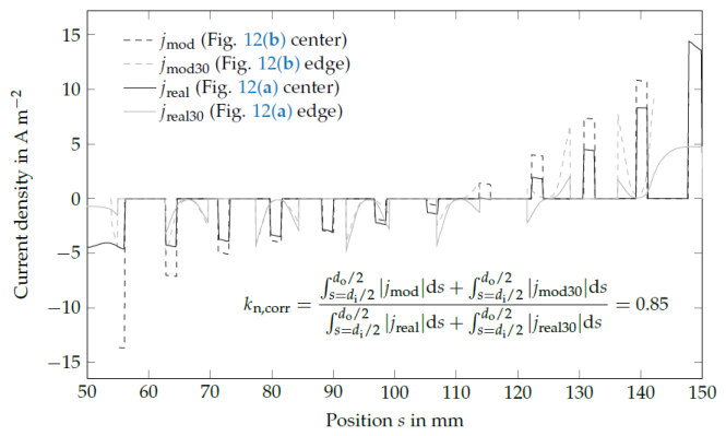
Figure 15.
Measured torque characteristic at (markers) and torque characteristics as a result of the simulation using the 2D reluctance model accounting for the measured temperature of the perforated sheets (dash-dotted), accounting for the correction of the Russell-Norsworthy factor (dashed), and accounting for both the temperature and the correction of the Russell-Norsworthy factor (solid).
Figure 15.
Measured torque characteristic at (markers) and torque characteristics as a result of the simulation using the 2D reluctance model accounting for the measured temperature of the perforated sheets (dash-dotted), accounting for the correction of the Russell-Norsworthy factor (dashed), and accounting for both the temperature and the correction of the Russell-Norsworthy factor (solid).
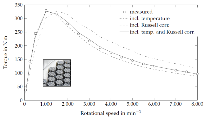
Figure 16.
Measured torque characteristic of the ECB with hex. Cluster structure at (markers) and simulated characteristics of the 2D reluctance model accounting for the measured sheet temperatures (solid), compared to the characteristics for with and with . The band shows the resulting uncertainty range of the overall model.
Figure 16.
Measured torque characteristic of the ECB with hex. Cluster structure at (markers) and simulated characteristics of the 2D reluctance model accounting for the measured sheet temperatures (solid), compared to the characteristics for with and with . The band shows the resulting uncertainty range of the overall model.
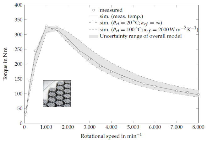
Figure 17.
Measured torque characteristic of the ECB with PIN structure at (markers) and simulated characteristics of the 2D reluctance model accounting for the measured sheet temperatures (solid), compared to the characteristics for with and with . The band shows the resulting uncertainty range of the overall model.
Figure 17.
Measured torque characteristic of the ECB with PIN structure at (markers) and simulated characteristics of the 2D reluctance model accounting for the measured sheet temperatures (solid), compared to the characteristics for with and with . The band shows the resulting uncertainty range of the overall model.
Disclaimer/Publisher’s Note: The statements, opinions and data contained in all publications are solely those of the individual author(s) and contributor(s) and not of MDPI and/or the editor(s). MDPI and/or the editor(s) disclaim responsibility for any injury to people or property resulting from any ideas, methods, instructions or products referred to in the content. |
© 2026 by the authors. Licensee MDPI, Basel, Switzerland. This article is an open access article distributed under the terms and conditions of the Creative Commons Attribution (CC BY) license (http://creativecommons.org/licenses/by/4.0/).
Copyright: This open access article is published under a Creative Commons CC BY 4.0 license, which permit the free download, distribution, and reuse, provided that the author and preprint are cited in any reuse.