

Submitted:
29 August 2026
Posted:
31 August 2026
You are already at the latest version
Abstract
Embedding a trained sheet-metal localisation surrogate inside a finite element (FEM) solver requires consistent predictions irrespective of the solver's strain-increment count, which is difficult to control in non-linear explicit codes. We re-implement in Fortran a trained recurrent neural network (RNN) damage criterion, previously validated only in Python/TensorFlow, and embed it as a live fracture criterion inside an Abaqus/Explicit user material subroutine (VUMAT). Two architectures are compared: a SimpleRNN and the proposed Consistent RNN (ConsRNN), whose transition function is designed so that predictions converge under path refinement rather than drifting with the increment count. Both are trained on bilinear strain paths and evaluated under varying discretisations and nonlinear histories. ConsRNN converges under refinement, at a substantial fixed-resolution accuracy cost on multilinear paths, whereas SimpleRNN predictions drift, disqualifying it for embedding. Deployed at structural scale, the embedded ConsRNN governs element deletion in a clamped steel plate and reaches the same peak force and displacement as an established two-parameter fracture criterion, an agreement expected by construction, with responses diverging only on the post-peak softening branch. The results establish discretisation consistency as the decisive property for embedding recurrent surrogates, and report, to the best of our knowledge, the first such embedding of a customised, non-standard-transition recurrent cell.
Keywords:
consistent recurrent neural networks
; surrogate modelling
; finite element method
; Abaqus/VUMAT
; path-dependent damage prediction
; computational mechanics
1. Introduction
Machine learning models are increasingly used as surrogates for the nonlinear relationship between deformation and mechanical response in engineering structures [1,2,3,4]. Instead of solving explicitly defined constitutive relations within finite element (FE) frameworks, data-driven models learn the input–output mapping directly from simulation data [2], motivating hybrid frameworks in which individual simulation components [5,6,7,8,9], or even entire simulation stages [10,11,12,13], are replaced by learned surrogates. Such models enable expensive simulation knowledge to be reused efficiently across analyses, while a single network formulation can represent multiple material classes with transferable learned representations [14]. In this spirit, Yatkın and Kõrgesaar [15] introduced a mapping from the deformation history of a material unit, sized to a large shell element, to its strain localisation response and demonstrated that this relationship can be learned directly from high-fidelity simulation data. In the present work, we take this localisation surrogate from offline validation to deployment, embedding a consistency-preserving recurrent network directly inside an explicit finite element solver.
Recurrent neural networks (RNNs) are natural candidates for learning such history-dependent mappings because their internal state advances across loading increments in the same way an FE solver advances its solution. Unlike fully connected neural networks, which require deformation history to be represented through hand-crafted state variables [16,17], recurrent architectures naturally retain historical information within their hidden state and have successfully learned homogenised constitutive behaviour [5], arbitrary non-proportional loading paths [18], and parametrized finite element simulations with varying mesh topologies [19]. However, predictive accuracy alone is insufficient for deployment as a finite element surrogate. Since explicit FE solvers determine their own increment sizes, surrogate predictions must remain consistent under temporal refinement. This has motivated the development of specialized recurrent transition functions capable of producing consistent estimates during simulation. Bonatti and Mohr [9] established self-consistency as a fundamental property of recurrent transition functions intended for use as surrogates inside FEM-based simulations, and Yatkin et al. [20] showed that any sequential learning architecture deployed as a surrogate must satisfy the truncation and consistency requirements.
This observation motivated several consistency-preserving recurrent formulations, including the Linearized Minimal State Cell [9], its rate- and temperature-dependent extension [21], recurrent surrogates for coupled plasticity and fracture in composites [22], and self-consistent gated recurrent units with fewer parameters [23]. Building upon this direction, our earlier studies [24,25,26] progressively extended the localisation surrogate to recurrent architectures, culminating in the Consistent Recurrent Neural Network (ConsRNN) [27]. ConsRNN differs from the Linearized Minimal State Cell in construction. The LMSC achieves self-consistency by learning a compact internal state whose update rule embeds physics-motivated variables tailored to the constitutive response. ConsRNN, in contrast, retains a standard recurrent hidden state and secures consistency purely through its mathematical design: a norm-scaled convex-combination state-transition update which can be interpreted as an explicit-Euler discretisation of an arc-length neural ordinary differential equation. Because consistency follows from the transition function itself rather than from embedded physical quantities, the property is architecture-intrinsic and transfers across problem settings, as demonstrated in Yatkin et al. [27] on two independent datasets. Beyond satisfying the consistency and truncation requirements for sequential surrogates [20], ConsRNN demonstrated consistent damage initiation predictions under varying increment counts on both synthetic and FEM-generated data, including the elastoplastic benchmark of Bonatti and Mohr [28]. Rather than serving as a replacement for empirical fracture criteria, ConsRNN introduces an additional learned information layer by compressing the localisation response of high-fidelity solid-element simulations into a fixed set of pre-trained network weights, learned offline rather than approximated at run time by a hand-calibrated criterion, thereby improving predictive accuracy while remaining compatible with arbitrary solver time discretisations. ConsRNN therefore provides a validated, consistency-preserving recurrent surrogate for history-dependent structural analysis.
Surrogate development, however, does not end with defining a mapping and training an architecture. An equally important challenge is deployment inside a finite element solver, where the trained network must execute incrementally while preserving its internal state across solver-driven time steps. Although recurrent surrogates for history-dependent material response have demonstrated promising offline predictive capability, comparatively little attention has been given to embedding customised recurrent architectures into production FE codes. Existing deployment approaches either rely on automated Keras-to-Fortran frameworks, which support only standard neural network layers [29,30], or hard-code neural network inference directly in Fortran [31,32]. In the latter case, however, the embedded networks are memoryless, with path dependence supplied by the surrounding physics-based formulation rather than by the network itself. To the best of our knowledge, no previous study has embedded a customised, consistency-preserving recurrent architecture, whose non-standard transition function falls outside existing deployment frameworks, into a structural-scale finite element simulation.
The present paper closes this gap. We follow the hard-coding strategy and apply it to the Consistent Recurrent Neural Network (ConsRNN) [27], previously validated only in Python/TensorFlow. The architecture is first optimised through Bayesian hyperparameter tuning, then reimplemented entirely in pure Fortran, with the learned weights transferred directly into an Abaqus VUMAT. As a comparison baseline we choose the SimpleRNN, which shares the same simple recurrent construction as ConsRNN without gating mechanisms, providing a more direct comparison than the gated LSTM and GRU architectures used by Bonatti and Mohr [9]. We demonstrate that the consistency property of ConsRNN is preserved under solver-driven computation with varying incremental step sizes, whereas the SimpleRNN baseline exhibits increment-dependent behaviour and is therefore unsuitable for explicit finite element analysis. The embedded surrogate is further evaluated against the established two-parameter (2FS) fracture criterion, demonstrating that ConsRNN can serve as a state-carrying surrogate damage predictor for history-dependent structural simulations while introducing an additional learned information layer through knowledge transferred from high-fidelity solid-element simulations.
The remainder of the paper is organised as follows. Section 2 presents the optimisation of the ConsRNN and SimpleRNN architectures through Bayesian hyperparameter tuning. Section 3 describes the pure-Fortran implementation and the transfer of learned weights into the Abaqus VUMAT. Section 4 presents the numerical experiments, comparing the embedded ConsRNN with the SimpleRNN baseline and the 2FS fracture criterion. Section 5 concludes the paper and outlines future work.
2. Neural Network Model Evaluation and Hyperparameter Tuning
Before deployment within the FEM solver, the proposed neural network architectures are first developed and evaluated through a standard machine learning workflow. The workflow comprises data analysis, architecture design, Bayesian hyperparameter optimization, and comprehensive qualitative and quantitative performance evaluation to ensure a reproducible comparison between the candidate models. The following subsections describe each stage of this workflow and motivate the selection of the architecture used for the subsequent Fortran implementation.
2.1. Path Dependent Damage Prediction Using Bilinear Loading Dataset
In an earlier study [15], we used fine solid-element simulations to understand how in-plane deformation history affects damage evolution and subsequent localisation. A bilinear loading path was defined in terms of the principal major and minor strain and orientation angle, and a total of 19,098 distinct bilinear loading paths were simulated. Each path comprises two linear segments and an orientation angle, discretised into 400 increments. The simpleRNN and ConsRNN architectures (details in the next section) were trained on this dataset, split into 13,367 training, 2,866 validation, and 2,865 test paths. The validation set guided model selection during hyperparameter tuning, and final performance was reported on the held-out test set using the best-trained weights.
For further testing, 240 additional bilinear paths were generated and discretised at increment counts different from the original 400, which were used to assess both the consistency and the accuracy of the damage estimates, along individual loading paths and on the resulting forming limit curves. The bilinear-trained models were also evaluated in Python on more complex paths of three, four, and five linear segments. This test was motivated by the nature of structural simulations, where a single element may follow a complex, history-dependent loading path drawn from an effectively unbounded set of scenarios. Accordingly, two complementary evaluations were carried out. First, the trained models were embedded in the Abaqus/VUMAT framework to study their behaviour in structural simulations, and second, the bilinear-trained models were separately assessed on multilinear loading paths in Python.
Here is a small numerical guard that keeps the logarithm bounded as .
2.2. Architectures
In the previous study [20], we showed that conventional recurrent architectures such as GRU and LSTM fail to satisfy the consistency requirements of path-dependent deformation. Furthermore, their gating mechanisms complicate direct implementation within a fixed-form Fortran VUMAT, increase the computational cost, and make hard-coded deployment of a trained model more challenging. In contrast, the SimpleRNN and ConsRNN cells share the same single recurrent transition and similar architectural simplicity, while matching in depth, capacity, and the absence of gating mechanisms, making the SimpleRNN a natural baseline for evaluating the proposed consistency-preserving transition formulation. We therefore built two single-layer recurrent architectures based on the SimpleRNN and ConsRNN cells to enable a controlled comparison. The two models are not, however, an isolated test of the cell equation alone: the SimpleRNN ingests the accumulated strains together with the loading orientation , whereas the ConsRNN ingests the normalised strain increments. Consequently, the input representation, input dimensionality, and normalisation strategy also differ between the two architectures. The comparison should therefore be interpreted as an evaluation of two complete surrogate formulations rather than as an isolated comparison of the transition function itself. A single-layer SimpleRNN architecture also proved sufficient to learn the bilinear deformation paths over 400 increments at low computational cost. We therefore restricted both architectures to a single recurrent layer and tuned each through repeated training runs.
The two cells differ in their inputs and in the transition functions used to update the state vectors. The SimpleRNN architecture takes the accumulated minor () and major () strains together with the loading orientation at each time step t, as shown in Figure 1 (a). The orientation is evaluated from the strain increments through , the ratio of the minor- to major-strain increment, following the convention used throughout this work. The ConsRNN architecture instead takes the incremental strain differences (, ) at each time step t, defined as the change in major and minor strain from the previous time step to the current time step t as shown in Figure 1 (b). In both cases the strains are principal plastic strains, and in the finite element implementation the network is advanced only on plastic increments: an elastic increment leaves the network state and the predicted damage unchanged. For both models, the target damage was mapped through the invertible function in Eq. (1) during training, while predictions were mapped back to the original damage scale at inference using Eq. (2).
In Table 1, denotes the cell input at time step t, that is, the strain increments for ConsRNN and the accumulated strains with orientation for SimpleRNN. Further, is its normalised form, the guarded Euclidean norm of the input increment, the recurrent state, and the transition activation obtained by applying the tanh nonlinearity to the affine combination of input and previous state. The matrices and are the trainable input and recurrent weights, the output weight, and b the bias; these parameters are learned during training rather than prescribed analytically. Here denotes the Euclidean norm of the input increment and the sigmoid function. The bounds entering act purely as numerical safeguards, the lower one against division by zero and the upper one against pathologically large increments. All strain increments encountered in this work satisfy , so throughout and the state update reduces to the unguarded form used in Eq. (4).
2.3. SimpleRNN Based Neural Network Architectures
The first architecture pairs the Keras/TensorFlow [33] SimpleRNN cell, whose update follows the standard formulation given in Table 1, with a single fully connected output layer using sigmoid activation. Its inputs are the accumulated minor and major strains and together with orientation , supplied at each time step through the mapping in Figure 1 (a). Recall that, unlike ConsRNN, the cell operates on the accumulated strains rather than on their increments. Each candidate model was trained for 100 epochs, and the hyperparameters were tuned through Bayesian optimisation over 20 trials, jointly searching the learning rate, batch size, and number of hidden units; the trial-by-trial progression is reported in Figure 2.
The best configuration uses 256 hidden units, a learning rate of , and a batch size of 16, yielding a mean squared error of 0.0010 on the training set and 0.0008 on the validation set (Figure 2). The close train–validation agreement indicates a well-conditioned fit; generalisation is assessed separately on the held-out test set (Table 2).
2.4. ConsRNN Based Neural Network Architectures
The consistency property of the ConsRNN cell follows from its transition function, which differs from that of SimpleRNN cell, see Table 1. Rather than taking the accumulated strains directly, the cell operates on the strain increments between successive time steps: it forms a candidate state, subtracts the previous state, and scales the difference by the Euclidean norm of the input increment before applying the update. Because each state advance is proportional to the increment norm, the accumulated prediction over a fixed path converges as the increment size is refined rather than drifting with the number of increments a property we refer to as discretisation consistency: convergence of the prediction under refinement of the discretisation of a fixed strain path.
The second architecture replaces the SimpleRNN cell with the ConsRNN cell defined in Table 1, followed by a single fully connected output layer using sigmoid activation. Its inputs are the strain increments and between successive time steps, supplied through the mapping in Figure 1(b). Following the same protocol as for the SimpleRNN, each candidate model was trained for 100 epochs and the hyperparameters were tuned through Bayesian optimisation over 20 trials, jointly searching the number of hidden units in , the learning rate on a log-uniform scale over , and the batch size in ; the trial-by-trial progression is reported in Figure 3.
The best configuration uses 256 hidden units, a learning rate of , and a batch size of 16, yielding a mean squared error of 0.0006 on both the training and validation sets (Figure 3). As with the SimpleRNN, the close train–validation agreement indicates a well-conditioned fit; generalisation is assessed separately on the held-out test set (Table 2).
Figure 4 places the two searches side by side. The SimpleRNN attains consistently low validation MSE across trials, whereas the ConsRNN shows larger trial-to-trial variability; the best configuration of the search overall is nonetheless a ConsRNN model, at 0.0006 against 0.0008 for the best SimpleRNN.
Although the lowest validation MSE was obtained with a batch size of 16, this configuration showed reduced accuracy at increment counts away from the 400-increment training resolution, while still preserving discretisation consistency. A configuration with batch size 256 achieved comparable consistency together with higher accuracy across all tested increment counts, and was therefore selected for the results reported in the remainder of this study.
2.5. Held-Out Test-Set Performance
The held-out test set results, summarized in Table 2, are consistent with the hyperparameter optimisation results on the bilinear loading dataset: the lowest-validation-MSE ConsRNN architecture outperforms the corresponding SimpleRNN architecture on every metric and on both output scales. On the converted scale, ConsRNN reduces the RMSE from to and the MAE from to , and raises the coefficient of determination from to . The same ordering holds on the original damage scale, where ConsRNN lowers the RMSE from to and improves from to .
The advantage extends to the tail of the error distribution: the 95th-percentile absolute error, which characterizes worst-case behaviour across the test paths, is also lower for ConsRNN on both scales ( versus on the converted scale, and versus on the damage scale). ConsRNN therefore fits the typical paths more accurately while remaining more reliable on the difficult cases. When the lowest-validation-MSE model of each architecture is selected and evaluated once on the untouched test set, ConsRNN is the more accurate surrogate of the two.
These results characterise the two architectures at their respective validation optima. As noted in Section 2.4, the ConsRNN configuration carried forward to the Fortran implementation and all subsequent experiments uses batch size 256, selected for its accuracy across increment counts rather than for its validation MSE at the training resolution.
2.6. Localisation Predictions for Bilinear Paths
To examine how the predicted localisation points depend on temporal resolution, we evaluated both trained architectures in Python/TensorFlow along a single bilinear deformation path, discretised at 400, , , and increments (Figure 5). The path consists of a first segment of length with direction and a second segment of length with . The ground-truth localisation point, marked by the empty circle in each panel, is obtained directly from the finite element simulation of this path, in which localisation occurs at increment of . The path is held fixed across all four panels, so that the only quantity changing between them is the number of increments used to traverse the identical strain history.
As the increment count increases, the SimpleRNN predictions drift progressively away from the ground-truth localisation point: at the training resolution of 400 increments the prediction is accurate, but at higher increment counts it departs visibly from the reference. The ConsRNN predictions, in contrast, remain close to and converge as the resolution is refined. This drift-free behaviour reflects the discretisation consistency built into the ConsRNN transition function: because each state advance is scaled by the norm of the strain increment, the accumulated prediction converges under refinement toward a value set by the path itself rather than by how finely it is sampled. It is this property that makes the surrogate usable across the varying, solver-dictated step sizes encountered in FE simulations, where the increment count cannot be prescribed by the user. The two architectures also differ in their input representation, not only in the transition function, so this contrast reflects the two complete designs rather than the transition function in isolation.
2.7. Forming Limit Curve (FLC) Predictions
The two selected architectures, the deployed ConsRNN (batch size 256) and the SimpleRNN, were used to predict localisation points that define two Forming Limit Curves (FLCs), shown in Figure 6. Each FLC is traced by fixing the first linear segment and sweeping the direction of the second segment: the first FLC fixes the first segment at length with direction , and the second at with . In both cases the second segment is held at fixed length while its direction is varied across 40 values, each value yielding one point on the curve. Here denotes the ratio of the minor- to major-strain increment, following the convention used throughout this work. Each path was simulated at increments and then downsampled to , , and 400 increments for prediction, so that the FLCs probe both accuracy and discretisation consistency. The ground-truth localisation points were obtained from Marciniak–Kuczyński finite element simulations in Abaqus of these bilinear paths, following the dataset described in Section 2.1, with the localisation strain read directly from each simulated path. These reference localisations are plotted alongside the SimpleRNN and ConsRNN predictions.
As Figure 6 shows, the ConsRNN-based architecture outperforms the SimpleRNN in both accuracy and consistency. It is nonetheless worth noting that the SimpleRNN predictions are far more consistent than those of the GRU model examined in the previous study [27]. This difference comes mainly from the theoretical structure of the GRU transition function, which includes a gating mechanism [34]. While this mechanism improves learning ability and accuracy, it also reduces the consistency of the estimations, as observed in the results in the previous study [27].
2.8. Localisation Predictions for Multilinear Paths
Although both architectures were trained only on bilinear loading paths, the mappings in Figure 1 (a) and (b) are history dependent and can therefore be applied to more complex multilinear paths. To test this, we generated multilinear paths of two, three, four, and five segments at 400 increments and predicted their localisation points with the bilinear-trained models. Each segment is specified by a length R and a direction expressed through , the ratio of the minor- to major-strain increment. The three-segment path is defined by the sequence ; the four-segment path by ; and the five-segment path by . Both architectures predict the localisation points as shown in Figure 7.
On these multilinear paths the SimpleRNN is the more accurate of the two, with an average MSE of versus for the ConsRNN (Figure 7). The ConsRNN evaluated here is the deployed batch-256 configuration carried forward to the Fortran implementation, rather than the lowest-validation-MSE batch-16 configuration reported in Table 2; as noted in Section 2.4, it was selected for accuracy across increment counts rather than at the 400-increment training resolution. At this fixed resolution the standard state update of the SimpleRNN is free to fit the training discretisation more closely. The results of this controlled out-of-distribution test reflect a genuine trade-off: at a single fixed increment count matching the training resolution, the convex, norm-scaled state update of the ConsRNN sacrifices accuracy to guarantee discretisation consistency, which the SimpleRNN does not provide. For deployment inside an Abaqus/VUMAT surrogate this trade-off favours the ConsRNN, because the solver assigns step sizes that can vary by orders of magnitude across elements and across increments. A SimpleRNN evaluated at resolutions away from its training increment count drifts from the correct localisation (Figure 5), and its fixed-resolution accuracy edge does not survive this variability, whereas the ConsRNN preserves both its consistency and its accuracy as the increment count increases. The ConsRNN is therefore the appropriate choice for FEM embedding, while the SimpleRNN remains competitive only where the increment count is fixed at the training resolution and known in advance.
3. Fortran Implementation
Neural networks are typically built and trained in TensorFlow or PyTorch, whereas the finite-element simulations in this work are run in Abaqus, where the constitutive response is supplied through Fortran user subroutines. Bridging the two ecosystems is not straightforward. Frameworks such as Neural-Fortran [35] and PyTorch-ABAQUS UMAT [36] have been proposed to couple TensorFlow or PyTorch with Fortran, but they are built around standard Keras and PyTorch layers, such as convolutional and recurrent layers. The Consistent Recurrent Neural Network (ConsRNN) developed in our previous work [27] uses a non-standard state-update mechanism that these bridging frameworks cannot represent directly.
We therefore reimplemented ConsRNN from scratch, reconstructing each computational block normalisation, state transition, state update, and damage output in native code. A similar block-by-block strategy has been adopted in related work [29,31]. This route gives full control over both the model and its numerical evaluation inside the solver. The workflow proceeds in three stages. The models are first trained in TensorFlow, and the trained weights are exported to text files. The forward pass is then replicated in NumPy from these weight files and matched against the TensorFlow output. Finally, each block is rewritten in pure Fortran, with the tensor outputs validated against the NumPy reference at every step shown in Figure 8. The result is a self-contained Fortran implementation of ConsRNN that integrates directly into Abaqus FEM simulations.
3.1. Python to Abaqus/Vumat Fortran
The incremental update mechanism of RNNs, in which a state vector is carried as memory across time steps, makes them well suited to material modelling, as emphasised by Mohr and co-workers [9,14,37]. Although architectures such as Transformers and CNNs can also represent deformation history, the recurrent update offers a decisive advantage for this purpose by advancing the state one increment at a time without storing or growing a sequence. This matches the structure of an explicit finite-element solver exactly. At each increment the RNN applies a transition function and then computes the output from the updated state, which is the same order of operations Abaqus performs at each material point. We therefore implemented the simulation environment from scratch in Python and translated the same logic into Fortran for embedding in the Abaqus VUMAT.
The trained SimpleRNN and ConsRNN one-layer architectures were first converted into pure scratch calculations, in which the damage predictions were matched between the TensorFlow model outputs and the NumPy-based scratch implementations. The same scratch implementations were subsequently rewritten in pure Fortran using the same inputs and tensor outputs.
The forward passes of the SimpleRNN- and ConsRNN-based architectures are summarized as pseudocode in Algorithms 1 and 2 (Appendix A), and the complete Python and Fortran implementations are openly available in the accompanying repository (see the Data Availability section). For both architectures, the Python and Fortran implementations produced identical damage outputs on the same input data, matching to five decimal places.
This cross-language validation established that the Fortran routines faithfully reproduce the trained networks. Only ConsRNN, however, was subsequently embedded in the Abaqus/VUMAT environment for the numerical experiments reported in this section. The earlier TensorFlow experiments in Section 2.7 showed that SimpleRNN does not satisfy the discretisation-consistency property: its predicted damage trajectory varies with the increment count even when the underlying strain path is identical. In an explicit finite-element simulation the increment count is dictated by the stable time step and can vary by orders of magnitude between runs, so a network with this property would yield damage predictions governed by the solver’s time-stepping rather than the physical deformation history. We therefore restricted the FEM-coupled experiments to ConsRNN, which is discretisation-consistent by construction.
The ConsRNN implementation is structured so that, once the simulation reaches a prescribed sampling frequency, the ConsRNN memory is updated by preserving the hidden-state vector within the StateEnv variables of the subroutine. The incremental differences between successive sampling instants are also stored, after which the update mechanism is applied and the damage is computed at each prescribed sampling point.
At each sampling instant the ConsRNN state vector is updated using the transition function presented in Table 1, and the corresponding damage value is computed. Crucially, no growing incremental input sequence of minor and major strain values is assembled and passed to the network, as is typical in TensorFlow-based implementations. The state vector is updated in place, the damage is computed immediately, and both are stored in the StateEnv variables.
In this way, the ConsRNN state vector and the damage evolution are consistently preserved and updated through the StateEnv structure across sampling instants. This allows ConsRNN to act as an FEM-compatible incremental solver while remaining memory-efficient and fully aligned with the way finite-element simulations operate in practice. This correspondence is the central objective of the present implementation: it enables ConsRNN to function as a physically consistent surrogate model that naturally follows the incremental strain evolution produced by the FEM simulation.
4. Numerical Experiments
Reproducing a forward pass in Fortran is not the same as operating inside a solver, where the network is driven by solver-chosen increments at a resolution that varies between elements and between runs, along strain paths never seen during training. Deployment also exposes behaviour that offline testing cannot reveal, since the subroutine must carry its state through the solver’s own memory management across thousands of material points without disrupting the analysis. The embedded surrogate is therefore evaluated in three stages: prescribed bilinear paths in single-element simulations, where the increment count is varied while the path is held fixed; element-level damage predictions in a full structural simulation, where each element follows its own non-proportional history; and finally the global force-displacement response with the surrogate governing element deletion, compared against the established 2FS criterion.
4.1. Single Element Simulations
Two different bilinear loading paths, previously introduced in [26], have been simulated in Abaqus using the VUMAT subroutine. The Fortran implementations of ConsRNN were tested by varying the loading frequencies. For each loading path, the strain increments extracted from the simulations were set to 400, 1000, 10000, 50000, 100000, and 200000. The corresponding results for each path are shown in Figure 9 and Figure 10. In addition, the localisation index ratio as a function of the number of increments is also included in the figures.
Each bilinear path consists of two linear segments in principal strain space, where each segment i is defined by an arc length and a direction expressed through , the ratio of the minor- to major-strain increment, following the convention used for the multilinear paths in Section 2.8. Step time is allocated to the segments in proportion to their lengths, such that the path is traversed at constant speed in strain space. The first path, shown in Figure 9, is defined by and . Its first segment () corresponds to nearly equibiaxial stretching, reaching , after which the loading direction changes abruptly by into the second segment (), which drives the material toward the drawing side of the strain plane. The predicted localisation instant, expressed as the normalised increment ratio at which the damage indicator reaches unity, converges monotonically from at to for , a spread of across a 500-fold range of temporal resolution.
The second path, shown in Figure 10, is defined by and , and represents the reverse scenario. Its first segment () lies close to pure shear, driving the material deep into the drawing side of the strain plane and reaching , after which the loading direction changes by into the second segment (), which pulls the material back toward nearly equibiaxial stretching. Along this path the damage accumulates more slowly, and localisation is reached only near the end of the prescribed loading: the predicted ratio converges monotonically from at to for , a spread of , mirroring the consistency observed for the first path.
As can be seen from the results, although the predictions show a minor deviation for the coarsest case with 400 increments, ConsRNN consistently preserves the localisation point as the number of increments increases, regardless of whether localisation occurs in the middle of the deformation path or near its end. This behavior indicates that ConsRNN is well suited for incremental material evolution: its memory mechanism carries the accumulated damage information between increments, so the prediction depends on the loading path itself rather than on its temporal discretisation, effectively acting as an incremental solver.
4.2. Structural Simulation and Material Model
In contrast to single shell element simulations where the prescribed in-plane loading was applied to the element, the elements in actual structures are exposed to infinitely complex loading histories. Therefore, the goal of this section is to reveal how the implemented ML models behave under these conditions.
The structural model used in this analysis is a rectangular steel plate clamped along all of its boundaries and deformed by a prescribed out-of-plane displacement applied through a rigid indenter at its centre. The plate is discretised with four-node reduced-integration shell elements of 3 mm thickness, with three Gauss integration points through the thickness so that both membrane and bending response are captured. The analysis is carried out in Abaqus/Explicit, and the constitutive behaviour is supplied through a user-defined material subroutine (VUMAT). This setup exposes the elements to non-proportional, spatially varying loading histories that differ from the prescribed single-element paths used in the previous section, since the strain history experienced by each element depends on its position relative to the indenter and on the evolving deformation of the surrounding material.
The same material model is used as in the previous section. The steel is described by a rate-independent, isotropic elastic-plastic constitutive law formulated under the plane-stress assumption appropriate for shell elements. The elastic response is linear and isotropic, defined by the Young’s modulus E and the Poisson’s ratio . Plastic flow follows the von Mises (J2) yield condition with associated flow rule and isotropic hardening. The flow stress obeys a modified Swift hardening rule, in which the stress is held at the initial yield stress up to a Lüders plateau strain , beyond which it follows the power-law relation
where is the equivalent plastic strain, K and n are the hardening parameters, and the offset strain enforces continuity of the stress-strain curve at . The constitutive equations are integrated using a plane-stress-consistent return-mapping algorithm, in which the through-thickness strain component is recovered iteratively so that the zero normal-stress condition is enforced at every increment. The steel is modelled with GPa, , density 7850 kg/m3, MPa, MPa, and .
Ductile fracture is modelled with the two-factor-scaling (2FS) criterion [38], in which the equivalent fracture strain is interpolated between an upper bound given by the Modified Mohr–Coulomb (MMC) fracture locus [39] and a lower bound given by the Swift diffuse-necking strain, according to the ratio of the characteristic element length to the plate thickness. This two-factor scaling regularises the mesh dependence of strain localisation in coarsely meshed shell structures, since the localisation and fracture strains exhibit different element-size sensitivities [40]. Damage is accumulated through a linear rule as the integral of the equivalent plastic strain increment normalised by the current fracture strain, and fracture occurs when the accumulated damage reaches unity, at which point the element is removed from the mesh through the standard element-deletion procedure. Following the original formulation, a triaxiality cut-off of is applied, below which fracture is not predicted, since the Swift necking lower bound is defined only for .
4.3. ConsRNN Based Damage Predictions in Structural Simulation
In a structural simulation, the number of strain increments accumulated by an element throughout its deformation history depends on the element location, the local deformation severity, and the adaptive timestep strategy of the solver. As a result, the number of increments can vary substantially between different elements and also between integration points within the same element. For a surrogate damage model to be practically useful within a simulation environment, its predictions should remain insensitive to such temporal-resolution variability.
Before assessing this consistency, the deployment itself was validated at the single integration-point level. Figure 11 and Figure 12 compare the embedded Fortran implementation against the Python reference at Element 2852, Integration Point 2, and Element 3089, Integration Point 3, respectively. In each case, the incremental strain components and computed inside the Fortran subroutine match the Python reference, obtained through numpy.diff of the strain trajectory, to file-write precision (panels (a) and (b)). The damage evolution predicted by the deployed Fortran ConsRNN follows the Python reference implementation throughout the entire loading history (panel (c)), with the pointwise difference between the two implementations remaining below across all output steps, 100 and 80 respectively (panel (d)). These results confirm faithful deployment of the trained ConsRNN model within the structural FEM context.
Building on this validated deployment, the embedded ConsRNN surrogate was examined at three elements and integration points extracted from the structural simulation, each with its own deformation history: Element 2852 at Integration Point 2 (Figure 13), Element 3089 at Integration Point 3 (Figure 14), and Element 2750 at Integration Point 1 (Figure 15). For each case, the same VUMAT simulation was sampled at three temporal resolutions (1000, 10000, and 23000 increments; 700, 7000, and 16000 increments; and 340, 3400, and 7800 increments, respectively), producing strain-increment sequences with substantially different time frequencies, as shown for the major and minor principal strain increments in panels (a) and (b) of each figure. The ConsRNN damage predictions were computed independently from these incremental principal strain histories, and the traditional monotonically increasing 2FS fracture criterion was extracted from the same simulation and overlaid along the deformation path for comparison. The increment axis was normalised between 0 and 1 to enable direct comparison across temporal resolutions and deformation histories.
Despite the substantially different temporal resolutions, the damage predictions in panel (c) of each figure remain highly consistent along the entire deformation path and converge toward similar final damage values: – for Element 2852, – for Element 3089, and – for Element 2750 across the respective increment counts. The overlaid 2FS criterion accumulates damage monotonically by construction and reaches different final values (, , and , respectively), since the two criteria evolve damage on different scales; the comparison is therefore qualitative rather than pointwise. Along each deformation path, the ConsRNN predictions follow the same overall growth trend as the 2FS reference, while exhibiting local non-monotonic segments that reflect the history-dependent nature of the learned damage evolution. In contrast to the 2FS curve, which is extracted at a single temporal resolution, the ConsRNN trajectories remain nearly indistinguishable across resolutions, which is precisely the property required for embedding within an explicit solver. This behavior directly supports the discretisation-consistency hypothesis of the proposed architecture under complex nonlinear deformation histories.
One important point that should be emphasized is that the ConsRNN architecture was trained only on bilinear loading paths, whereas the structural simulations contain significantly more complex and nonlinear deformation histories. Despite this distributional difference between training and testing conditions, the embedded surrogate still produces stable and temporally consistent damage predictions across varying increment counts. These observations demonstrate that the proposed ConsRNN-based pipeline can be directly integrated into a structural simulation environment and operate as an incremental surrogate solver inside the simulation loop. Naturally, further improvements in prediction accuracy are expected through the generation of more representative nonlinear training paths and more specialized training datasets. Nevertheless, the current results already demonstrate the feasibility of directly embedding a recurrent neural-network-based surrogate model into a structural simulation framework.
4.4. Global Force and Displacement Curve
The global force–displacement response is the primary measure against which fracture criteria in large-scale crash and collision analysis are validated, since it is the quantity most reliably recorded in physical experiments and the one that governs the predicted energy absorption of the structure. Its shape encodes the essential structural behaviour: the pre-peak branch reflects the combined elastic and plastic stiffness of the deforming members, the peak marks the onset of fracture and the loss of load-carrying capacity, and the post-peak softening branch captures the progressive failure and the residual resistance as elements are eroded. A surrogate damage model is therefore only of practical value if it can reproduce this response when embedded in a full structural simulation, where each element experiences a non-proportional loading history rather than a prescribed path. Recovering the force–displacement curve thus serves as the decisive test of whether the model has learned a physically meaningful damage evolution, and demonstrates that it can act as a drop-in replacement for a traditional fracture criterion within the solver.
Figure 16 compares the global force–displacement response of the structure under two erosion criteria: the traditional 2FS fracture criterion and the proposed ConsRNN surrogate, embedded directly into the VUMAT as the element-deletion criterion. The two responses are identical throughout the pre-peak regime: both simulations reach the same peak force of kN at the same displacement of mm, since the first element deletion occurs only beyond the peak, so that the two criteria govern identical solution paths up to the onset of failure. Both simulations accordingly exhibit the onset of load drop at the same displacement, indicating that structural failure initiates at the same stage of loading under either criterion. Beyond the peak, the curves diverge moderately, with the ConsRNN run settling to a lower residual load-carrying capacity than the 2FS run (a final force of kN versus kN at the end of the prescribed loading), reflecting a slightly more progressed element erosion on the post-peak softening branch. This level of agreement is notable given that the ConsRNN model was trained only on bilinear loading paths, yet here governs failure under the non-linear, complex strain histories produced by the full structural simulation. The result demonstrates that the proposed surrogate can be embedded as a live fracture criterion inside a finite-element solver and reproduce the global structural response of an established criterion, while operating as an incremental damage predictor rather than an offline post-processor.
The computational cost of the embedded surrogate was measured on the same structural analysis. Both simulations were run on identical hardware with four domains and four processors, over the same prescribed loading to a step time of , and both completed in increments, since the stable time increment is fixed by mass scaling and is therefore unaffected by the choice of erosion criterion. Under the 2FS criterion the analysis required s of user time and 255 s of wallclock time, against s and 250 s for the embedded ConsRNN, corresponding to approximately ms of user time per increment in both cases. The difference of roughly 1% lies within run-to-run variation, so the two criteria are computationally indistinguishable at this scale. This result follows from two features of the implementation: the network state is advanced only on plastic increments and at a prescribed sampling frequency rather than at every solver increment, and the 2FS criterion itself is not free, requiring evaluation of the Modified Mohr–Coulomb locus, the Swift diffuse-necking strain, and the stress triaxiality at each material point. The learned information layer carried by the surrogate is therefore obtained without a measurable computational penalty relative to an established analytical criterion.
4.5. Discussion of the Results and Current Limitations
The consistency of the ConsRNN predictions can be observed at several levels. For a single element under bilinear loading, Figure 9 and Figure 10 show that the estimated damage remains consistent across different increment discretisations of the same path. The same behaviour is seen at the single element, one integration point level for the deformation-history based predictions obtained from the structural simulation in Figure 13, Figure 14, and Figure 15, where the proposed transition-formula based architecture predicts consistent damage on non-linear loading paths, although it was trained only on bilinear paths. Notably, even though the incremental differences vary considerably along the non-linear paths under different discretisations, the consistency in the estimates is preserved, which is an important property for use within a structural simulation. Additionally, Figure 16 shows that the proposed surrogate model produces a force and displacement curve closely aligned with the traditional fracture criterion, indicating that the model is a promising alternative. Taken together, these results obtained inside the Abaqus/VUMAT environment support the central claim of this paper. Another behaviour that should be highlighted is that the predicted ConsRNN damage values occasionally decrease during certain stages of the deformation path before increasing again. This non-monotonic behaviour can be observed in particular near the final stages of Figure 13 and Figure 14. Physically, damage evolution is generally expected to be irreversible, and the predictions should therefore ideally evolve monotonically throughout the loading history. This behaviour originates directly from the current ConsRNN state-update formulation given in Table 1. In the present implementation, the transition activation is computed using a hyperbolic tangent function, and is therefore not constrained to remain larger than the previously accumulated state. From the update rule, the incremental state evolution can be expressed as
where is the transition activation and denotes the Euclidean norm of the strain-increment vector. Since , the sign of the state increment is determined entirely by the term . Consequently, whenever the transition activation becomes smaller than the accumulated state, that is , the state increment becomes negative and the predicted damage temporarily decreases. Enforcing physically compatible, monotonically increasing damage predictions while preserving the consistency property of the transition formulation is a non-trivial question that we identify as a direction for further research. The two requirements are not independent: the same update mechanism that makes the predictions insensitive to the discretisation of the strain path also allows the state increment to take a negative sign when the transition activation falls below the accumulated state. A constraint that simply forces the output to be non-decreasing could therefore interfere with the consistency that is central to the present formulation. A more principled treatment would instead seek a transition formula that is monotonic by construction, for example through an activation or accumulation rule that guarantees a non-negative state increment without altering the path-consistent behaviour. We regard the design of such a formulation, together with a study of its effect on the damage evolution and the resulting structural response, as a worthwhile topic for future work.
5. Conclusions
In this study, we embedded a surrogate Consistent Recurrent Neural Network (ConsRNN) directly within Abaqus finite element simulations through a Fortran VUMAT subroutine. The model was developed and trained in Python and TensorFlow on datasets extracted from finite element simulations, and the trained network was then evaluated natively within the solver, with its weights, hidden state, and incremental update computed in Fortran at every material point rather than through an external coupling interface. The in-solver implementation reproduced the reference Python predictions to within an agreement of order , confirming that the embedding preserves the trained model rather than approximating it. We further showed that ConsRNN operates as an incremental solver, carrying the learned material evolution between strain increments and producing a damage history that is consistent in time and largely independent of the discretisation of the strain path.
The approach was validated on prescribed strain paths using single element simulations and then assessed in full structural simulations of clamped shell plates, where each element follows a non-proportional loading history that differs in both shape and increment count. Although the network was trained only on bilinear loading paths, it predicted element-level damage under these more complex histories and reproduced a global force and displacement response in close agreement with the traditional 2FS fracture criterion. This indicates a degree of generalisation beyond the training regime, and demonstrates that a learned damage model can be carried through a structural analysis without re-evaluating a closed-form fracture locus at each step. Unlike a fixed analytical criterion, the surrogate accumulates damage from the deformation history itself, which offers a route to representing path-dependent behaviour and to modelling materials or loading regimes for which no closed-form criterion is readily available.
More broadly, this work demonstrates a complete and reproducible workflow for developing a machine learning surrogate, training it on data from physical simulations, and deploying it directly inside an established finite element solver through a hard-coded user subroutine. We regard it as a representative example of how a trained ML model can be tested and operated within engineering simulation environments, and as a reference point for future efforts to integrate learned constitutive and damage models into physics-based solvers. Future work should extend the training data to richer loading histories and quantify the model’s accuracy and robustness across a wider range of structural configurations and material systems.
6. Patents
A US provisional patent application, No. 63/953,756, has been filed covering aspects of the methodology reported in this manuscript.
Author Contributions
Muhammed Adil Yatkın: conceptualization, methodology, software, validation, formal analysis, investigation, visualization, writing (original draft). Mihkel Kõrgesaar: conceptualization, methodology, supervision, funding acquisition, writing (review and editing). Hasan Kurban: methodology, writing (review and editing).
Funding
Estonian Research Council, grant PSG754 (Coupled simulation model for ship crashworthiness assessment).
Institutional Review Board Statement
Not applicable.
Informed Consent Statement
Not applicable.
Data Availability Statement
The trained ConsRNN model weights, the standalone NumPy and Fortran implementations, the Abaqus/Explicit VUMAT deployment codes, and the evaluation scripts used to produce the figures in this paper are openly available on Zenodo at https://doi.org/10.5281/zenodo.21207967.
Acknowledgments
The corresponding author wishes to express sincere gratitude to Mr. Valeh Farzaliyev for valuable discussions and insightful comments.
Conflicts of Interest
The authors declare a US provisional patent application, No. 63/953,756, relating to the methodology described in this manuscript. The funders had no role in the design of the study; in the collection, analyses, or interpretation of data; in the writing of the manuscript; or in the decision to publish the results.
Appendix A. Pseudocode of the Damage-Evolution Networks
Algorithms 1 and 2 summarize the forward passes of the baseline SimpleRNN and the proposed ConsRNN models as executed at each material point. The notation follows Table 1: and denote the input and recurrent weight matrices, the output weight, and b the corresponding biases. The full NumPy and Fortran reference implementations, the trained model weights, and the Abaqus/Explicit VUMAT deployment codes are openly available in the repository at https://doi.org/10.5281/zenodo.21207967.
| Algorithm 1 SimpleRNN damage evolution (baseline) |
|
| Algorithm 2 ConsRNN damage evolution |
|
References
- Bonatti, C.; Berisha, B.; Mohr, D. From CP-FFT to CP-RNN: Recurrent neural network surrogate model of crystal plasticity. Int. J. Plast. 2022, 158, 103430. [Google Scholar] [CrossRef]
- Khandelwal, S.; Basu, S.; Patra, A. A Machine Learning-based surrogate modeling framework for predicting the history-dependent deformation of dual phase microstructures. Mater. Today Commun. 2021, 29, 102914. [Google Scholar] [CrossRef]
- Suttakul, P.; Vo, D.; Fongsamootr, T.; Wanison, R.; Mona, Y.; Katongtung, T.; Tippayawong, N.; Thawon, I. The role of machine learning for insight into the material behavior of lattices: a surrogate model based on data from finite element simulation. Results Eng. 2024, 23, 102547. [Google Scholar] [CrossRef]
- Yarmohammadian, R.; Put, F.; Van Coile, R. Physics-Informed Surrogate Modelling in Fire Safety Engineering: A Systematic Review. Appl. Sci. 2025, 15. [Google Scholar] [CrossRef]
- Mozaffar, M.; Bostanabad, R.; Chen, W.; Ehmann, K.; Cao, J.; Bessa, M. Deep learning predicts path-dependent plasticity. Proc. Natl. Acad. Sci. 2019, 116, 26414–26420. [Google Scholar] [CrossRef]
- Wu, L.; Kilingar, N.G.; Noels, L.; et al. A recurrent neural network-accelerated multi-scale model for elasto-plastic heterogeneous materials subjected to random cyclic and non-proportional loading paths. Comput. Methods Appl. Mech. Eng. 2020, 369, 113234. [Google Scholar] [CrossRef]
- Ghavamian, F.; Simone, A. Accelerating multiscale finite element simulations of history-dependent materials using a recurrent neural network. Comput. Methods Appl. Mech. Eng. 2019, 357, 112594. [Google Scholar] [CrossRef]
- Maia, M.; Rocha, I.; Kerfriden, P.; van der Meer, F. Physically recurrent neural networks for path-dependent heterogeneous materials: Embedding constitutive models in a data-driven surrogate. Comput. Methods Appl. Mech. Eng. 2023, 407, 115934. [Google Scholar] [CrossRef]
- Bonatti, C.; Mohr, D. On the importance of self-consistency in recurrent neural network models representing elasto-plastic solids. J. Mech. Phys. Solids 2022, 158, 104697. [Google Scholar] [CrossRef]
- Flaschel, M.; Kumar, S.; De Lorenzis, L. Unsupervised discovery of interpretable hyperelastic constitutive laws. Comput. Methods Appl. Mech. Eng. 2021, 381, 113852. [Google Scholar] [CrossRef]
- Carrara, P.; Ortiz, M.; De Lorenzis, L. Data-driven rate-dependent fracture mechanics. J. Mech. Phys. Solids 2021, 155, 104559. [Google Scholar] [CrossRef]
- Kirchdoerfer, T.; Ortiz, M. Data-driven computational mechanics. Comput. Methods Appl. Mech. Eng. 2016, 304, 81–101. [Google Scholar] [CrossRef]
- Eggersmann, R.; Kirchdoerfer, T.; Reese, S.; Stainier, L.; Ortiz, M. Model-free data-driven inelasticity. Comput. Methods Appl. Mech. Eng. 2019, 350, 81–99. [Google Scholar] [CrossRef]
- Bonatti, C.; Mohr, D. One for all: Universal material model based on minimal state-space neural networks. Sci. Adv. 2021, 7, eabf3658. [Google Scholar] [CrossRef]
- Yatkın, M.A.; Kõrgesaar, M. Machine learning enabled identification of sheet metal localization. Int. J. Solids Struct. 2024, 288, 112592. [Google Scholar] [CrossRef]
- Palau, T.; Kuhn, A.; Nogales, S.; Böhm, H.J.; Rauh, A. A neural network based elasto-plasticity material model. In Proceedings of the CD-ROM Proceedings of the 6th European Congress on Computational Methods in Applied Sciences and Engineering (ECCOMAS 2012), 2012; TU Wien; p. 10. [Google Scholar]
- Gorji, M.B.; Mohr, D. Towards neural network models for describing the large deformation behavior of sheet metal. Proc. IOP Conf. Ser. Mater. Sci. Eng. 2019, Vol. 651, 012102. [Google Scholar] [CrossRef]
- Gorji, M.B.; Mozaffar, M.; Heidenreich, J.N.; Cao, J.; Mohr, D. On the potential of recurrent neural networks for modeling path dependent plasticity. J. Mech. Phys. Solids 2020, 143, 103972. [Google Scholar] [CrossRef]
- Greve, L.; van de Weg, B.P. Surrogate modeling of parametrized finite element simulations with varying mesh topology using recurrent neural networks. Array 2022, 14, 100137. [Google Scholar] [CrossRef]
- Yatkin, M.A.; Kõrgesaar, M.; Asan, V.M.; Romanoff, J.; Stuckner, J.; Kurban, H. Self-consistent recurrent neural network for path dependent deformation. Sci. Rep. 2026, 16, 20480. [Google Scholar] [CrossRef]
- Heidenreich, J.N.; Mohr, D. Extended minimal state cells (EMSC): Self-consistent recurrent neural networks for rate- and temperature dependent plasticity. Int. J. Plast. 2025, 188, 104305. [Google Scholar] [CrossRef]
- Girard, A.; Mohr, D. Recurrent neural network model predicting elasto-plasticity and matrix fracture in fiber-reinforced composites. Int. J. Solids Struct. 2026, 326, 113703. [Google Scholar] [CrossRef]
- Wu, L.; Noels, L. Self-consistency Reinforced minimal Gated Recurrent Unit for surrogate modeling of history-dependent non-linear problems: Application to history-dependent homogenized response of heterogeneous materials. Comput. Methods Appl. Mech. Eng. 2024, 424, 116881. [Google Scholar] [CrossRef]
- Yatkin, M.A.; Kõrgesaar, M. Fracture Estimation Based on Deformation History with Recurrent Neural Networks. In Proceedings of the 2023 International Conference on Machine Learning and Applications (ICMLA), 2023; pp. 1025–1030. [Google Scholar] [CrossRef]
- Yatkin, M.A.; Korgesaar, M.; Romanoff, J.; Stuckner, J.; Işlak, Ü.; Kurban, H. Exploring various sequential learning methods for deformation history modeling. In Proceedings of the International Conference on Engineering Applications of Neural Networks, 2025; Springer; pp. 168–180. [Google Scholar]
- Kõrgesaar, M.; Yatkin, M.A. Machine Learning Based Computational Models for Increased Accuracy and Enabling Digital Twins. Proc. Int. Conf. Offshore Mech. Arct. Eng. 2025, Vol. 88964, V007T14A014. [Google Scholar]
- Yatkın, M.A.; Kõrgesaar, M.; Işlak, Ü. A Topological Approach to Enhancing Consistency in Machine Learning via Recurrent Neural Networks. Appl. Sci. 2025, 15, 933. [Google Scholar] [CrossRef]
- Bonatti, C.; Mohr, D. Data for: On the Importance of Self-consistency in Recurrent Neural Network Models Representing Elasto-plastic Solids. 2021. [Google Scholar] [CrossRef]
- Pantalé, O.; Tize Mha, P.; Tongne, A. Efficient implementation of non-linear flow law using neural network into the Abaqus Explicit FEM code. Finite Elem. Anal. Des. 2022, 198, 103647. [Google Scholar] [CrossRef]
- Ott, J.; Pritchard, M.; Best, N.; Linstead, E.; Curcic, M.; Baldi, P. A Fortran-Keras Deep Learning Bridge for Scientific Computing. CoRR 2020, abs/2004.10652. [Google Scholar]
- Kessler, B.S.; El-Gizawy, A.S.; Smith, D.E. Incorporating Neural Network Material Models Within Finite Element Analysis for Rheological Behavior Prediction. J. Press. Vessel Technol. 2006, 129, 58–65. Available online: https://asmedigitalcollection.asme.org/pressurevesseltech/article-pdf/129/1/58/5683667/58_1.pdf. [CrossRef]
- Jang, D.K.; Fazily, P.; Yoon, J.W. Machine learning-based constitutive model for J2-plasticity. Int. J. Plast. 2021, 138, 102919. [Google Scholar] [CrossRef]
- Abadi, M.; Agarwal, A.; Barham, P.; Brevdo, E.; Chen, Z.; Citro, C.; Corrado, G.S.; Davis, A.; Dean, J.; Devin, M.; et al. TensorFlow: Large-Scale Machine Learning on Heterogeneous Systems, 2015. Software available from tensorflow.org. [CrossRef]
- Dey, R.; Salem, F.M. Gate-Variants of Gated Recurrent Unit (GRU) Neural Networks. CoRR 2017, abs/1701.05923. [Google Scholar]
- Curcic, M. A parallel Fortran framework for neural networks and deep learning. arXiv 2019, arXiv:cs. [Google Scholar]
- Suh, H.S.; Kweon, C.; Lester, B.; Kramer, S.; Sun, W. A publicly available PyTorch-ABAQUS UMAT deep-learning framework for level-set plasticity. Mech. Mater. 2023, 184, 104682. [Google Scholar] [CrossRef]
- Heidenreich, J.N.; Mohr, D. Recurrent neural network plasticity models: Unveiling their common core through multi-task learning. Comput. Methods Appl. Mech. Eng. 2024, 426, 116991. [Google Scholar] [CrossRef]
- Korgesaar, M. The effect of low stress triaxialities and deformation paths on ductile fracture simulations of large shell structures. Mar. Struct. 2019, 63, 45–64. [Google Scholar] [CrossRef]
- Zhang, S.; Wu, X.; Yang, M.; Ren, P.; Meng, X. Simulation of Fracture Performance of Die-Cast A356 Aluminum Alloy Based on Modified Mohr–Coulomb Model. Appl. Sci. 2023, 13. [Google Scholar] [CrossRef]
- Cho, Y.; Lee, C.; Yee, J.J.; Kim, D.K. Modeling of Ductile Fracture for SS275 Structural Steel Sheets. Appl. Sci. 2021, 11. [Google Scholar] [CrossRef]
Figure 1.
Input representations of the same bilinear loading path for the two architectures in principal strain space. The red marker highlights the state of deformation at time t. Panel (a) shows the input to the SimpleRNN and panel (b) the input to the ConsRNN. Both panels depict the same underlying loading path, but the SimpleRNN encodes it through the accumulated strain state whereas the ConsRNN encodes it through the incremental strain differences.
Figure 1.
Input representations of the same bilinear loading path for the two architectures in principal strain space. The red marker highlights the state of deformation at time t. Panel (a) shows the input to the SimpleRNN and panel (b) the input to the ConsRNN. Both panels depict the same underlying loading path, but the SimpleRNN encodes it through the accumulated strain state whereas the ConsRNN encodes it through the incremental strain differences.
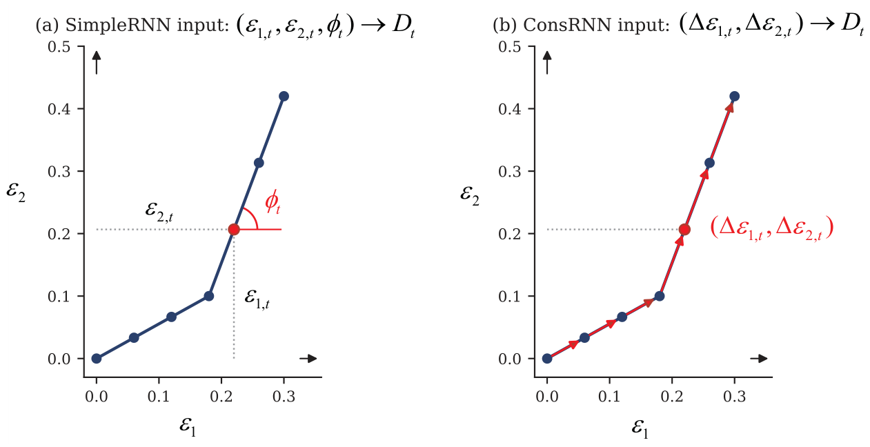
Figure 2.
Hyperparameter tuning of the SimpleRNN-based architecture over 20 Bayesian optimisation trials on the validation dataset. Each marker denotes one trial, positioned by hidden units and validation MSE, coloured by learning rate. The lowest MSE () uses 256 hidden units, learning rate , and batch size 16 (highlighted).
Figure 2.
Hyperparameter tuning of the SimpleRNN-based architecture over 20 Bayesian optimisation trials on the validation dataset. Each marker denotes one trial, positioned by hidden units and validation MSE, coloured by learning rate. The lowest MSE () uses 256 hidden units, learning rate , and batch size 16 (highlighted).
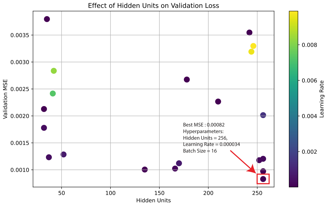
Figure 3.
Hyperparameter tuning of the ConsRNN-based architecture over 20 Bayesian optimisation trials on the validation dataset. Each marker denotes one trial, positioned by hidden units and validation MSE, with colour indicating the learning rate. The lowest MSE () is obtained with 256 hidden units, learning rate , and batch size 16 (highlighted); batch size 256 was selected for the study, as explained in the text.
Figure 3.
Hyperparameter tuning of the ConsRNN-based architecture over 20 Bayesian optimisation trials on the validation dataset. Each marker denotes one trial, positioned by hidden units and validation MSE, with colour indicating the learning rate. The lowest MSE () is obtained with 256 hidden units, learning rate , and batch size 16 (highlighted); batch size 256 was selected for the study, as explained in the text.
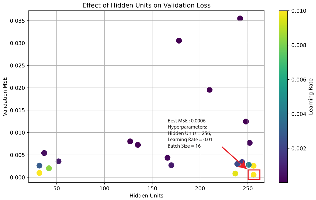
Figure 4.
Validation mean squared error (MSE) across the 20 Bayesian optimisation trials for the SimpleRNN and ConsRNN architectures. The SimpleRNN attains consistently low MSE across trials, whereas the ConsRNN exhibits larger trial-to-trial variability; nevertheless, the best-performing configuration overall is a ConsRNN model, reaching the lowest validation MSE of the search (0.0006 versus 0.0008 for the best SimpleRNN).
Figure 4.
Validation mean squared error (MSE) across the 20 Bayesian optimisation trials for the SimpleRNN and ConsRNN architectures. The SimpleRNN attains consistently low MSE across trials, whereas the ConsRNN exhibits larger trial-to-trial variability; nevertheless, the best-performing configuration overall is a ConsRNN model, reaching the lowest validation MSE of the search (0.0006 versus 0.0008 for the best SimpleRNN).
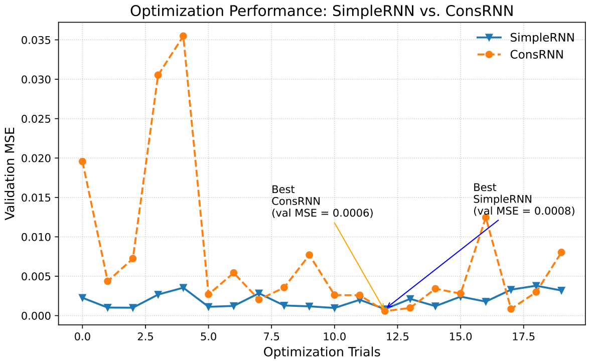
Figure 5.
Localisation predictions obtained from SimpleRNN and ConsRNN are compared under different numbers of increments. While increasing the number of increments causes SimpleRNN predictions to drift, ConsRNN predictions remain consistent.
Figure 5.
Localisation predictions obtained from SimpleRNN and ConsRNN are compared under different numbers of increments. While increasing the number of increments causes SimpleRNN predictions to drift, ConsRNN predictions remain consistent.
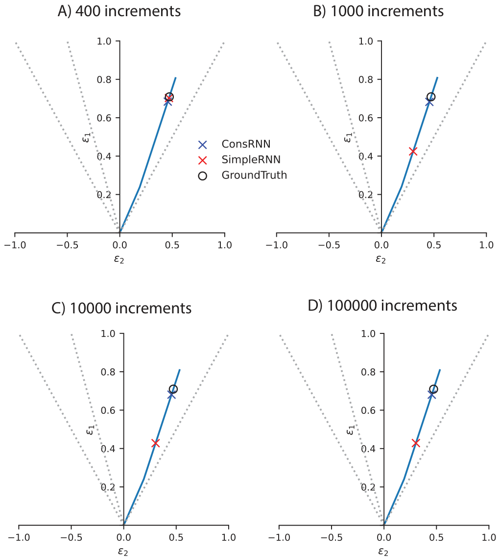
Figure 6.
FLC predictions from SimpleRNN and ConsRNN trained neural network architectures.
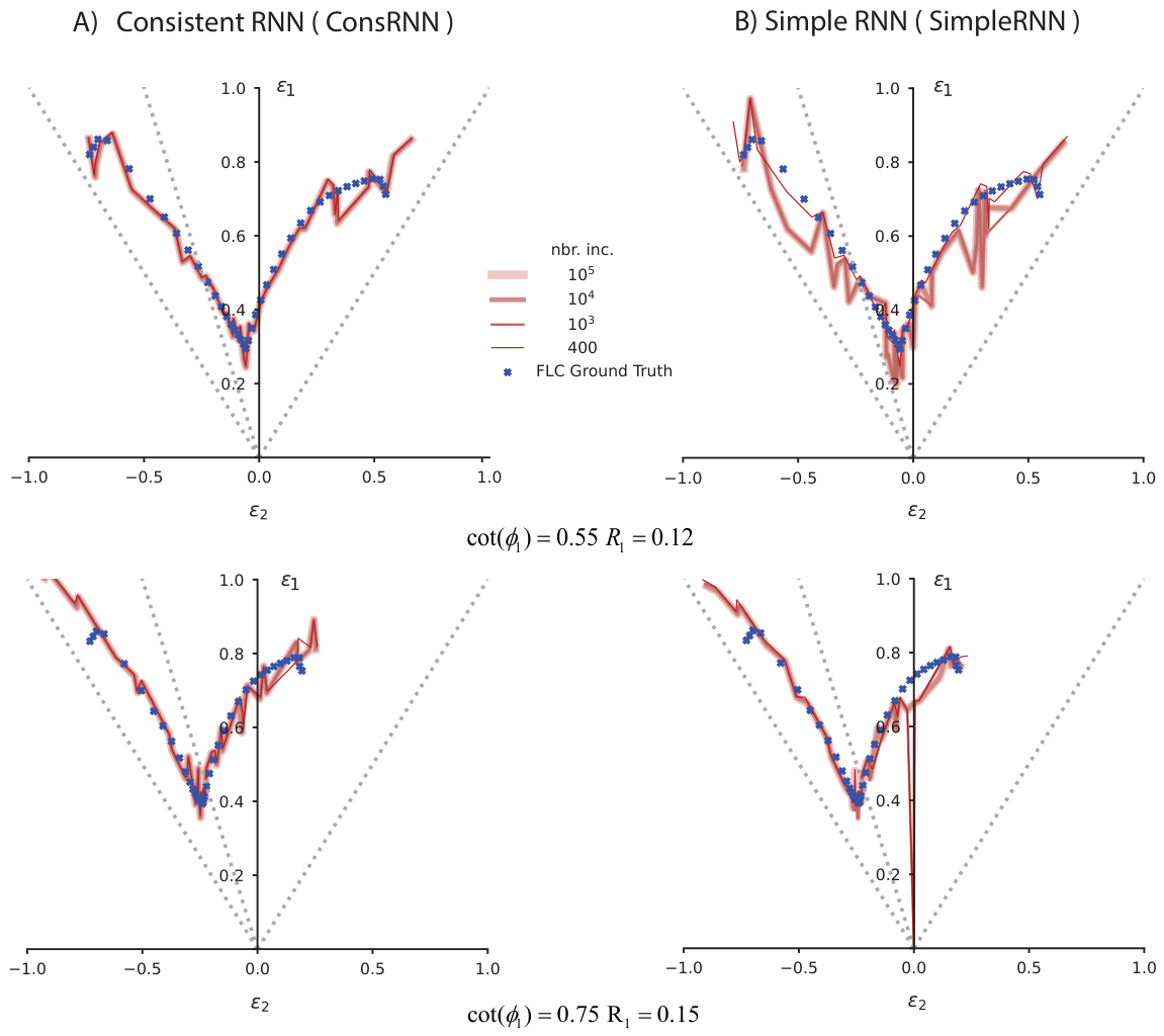
Figure 7.
Localisation predictions for multilinear paths (two to five segments) from the deployed ConsRNN (A, batch size 256) and the SimpleRNN (B) architectures over 400 increments. The black curve with filled markers is the reference forming limit curve from Figure 6. Circles: ground truth; crosses: predictions.
Figure 7.
Localisation predictions for multilinear paths (two to five segments) from the deployed ConsRNN (A, batch size 256) and the SimpleRNN (B) architectures over 400 increments. The black curve with filled markers is the reference forming limit curve from Figure 6. Circles: ground truth; crosses: predictions.
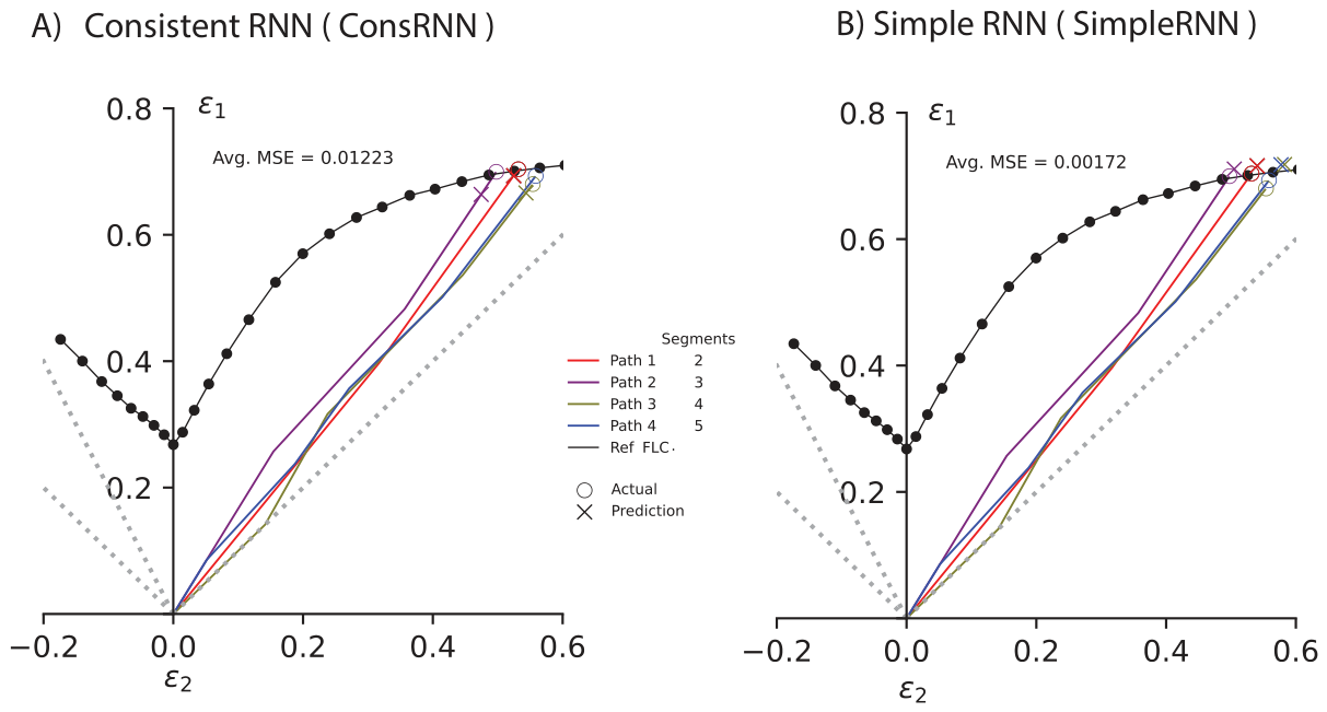
Figure 8.
Three-stage workflow for the Fortran implementation of the ConsRNN architecture: training in Python/TensorFlow, replication in NumPy, and rewriting in pure Fortran, validated against each other at every stage. The resulting code is embedded into the Abaqus VUMAT subroutine (Section 3).
Figure 8.
Three-stage workflow for the Fortran implementation of the ConsRNN architecture: training in Python/TensorFlow, replication in NumPy, and rewriting in pure Fortran, validated against each other at every stage. The resulting code is embedded into the Abaqus VUMAT subroutine (Section 3).
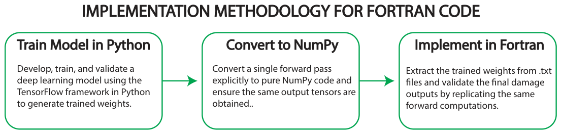
Figure 9.
Localisation predictions of ConsRNN embedded in Abaqus/Explicit for the first bilinear strain path (; ), evaluated at increment counts from 400 to 200,000. Markers denote the predicted localisation point.
Figure 9.
Localisation predictions of ConsRNN embedded in Abaqus/Explicit for the first bilinear strain path (; ), evaluated at increment counts from 400 to 200,000. Markers denote the predicted localisation point.
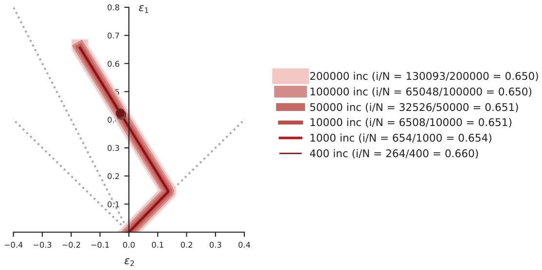
Figure 10.
Localisation predictions of ConsRNN embedded in Abaqus/Explicit for the second bilinear strain path (; ), evaluated at increment counts from 400 to 200,000. Markers denote the predicted localisation point.
Figure 10.
Localisation predictions of ConsRNN embedded in Abaqus/Explicit for the second bilinear strain path (; ), evaluated at increment counts from 400 to 200,000. Markers denote the predicted localisation point.
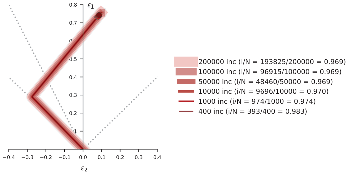
Figure 11.
Validation of the embedded ConsRNN at Element 2852, Integration Point 2 of the structural simulation: Fortran-computed strain increments and damage evolution against the Python reference.
Figure 11.
Validation of the embedded ConsRNN at Element 2852, Integration Point 2 of the structural simulation: Fortran-computed strain increments and damage evolution against the Python reference.
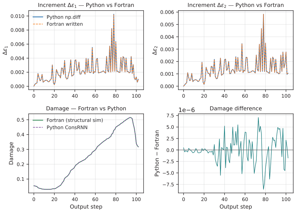
Figure 12.
Validation of the embedded ConsRNN at Element 3089, Integration Point 3 of the structural simulation: Fortran-computed strain increments and damage evolution against the Python reference.
Figure 12.
Validation of the embedded ConsRNN at Element 3089, Integration Point 3 of the structural simulation: Fortran-computed strain increments and damage evolution against the Python reference.
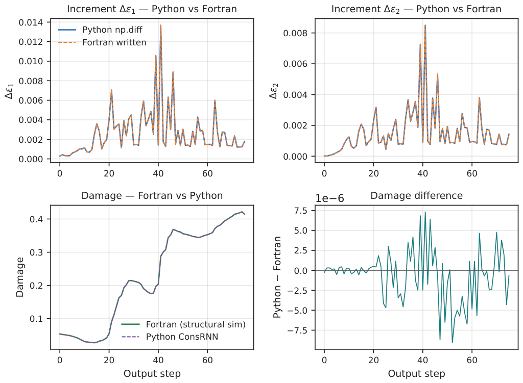
Figure 13.
ConsRNN damage predictions at Element 2852, Integration Point 2, sampled at three temporal resolutions (1000, 10000, and 23000 increments): (a) major and (b) minor principal strain increments; (c) damage evolution compared with the 2FS criterion.
Figure 13.
ConsRNN damage predictions at Element 2852, Integration Point 2, sampled at three temporal resolutions (1000, 10000, and 23000 increments): (a) major and (b) minor principal strain increments; (c) damage evolution compared with the 2FS criterion.
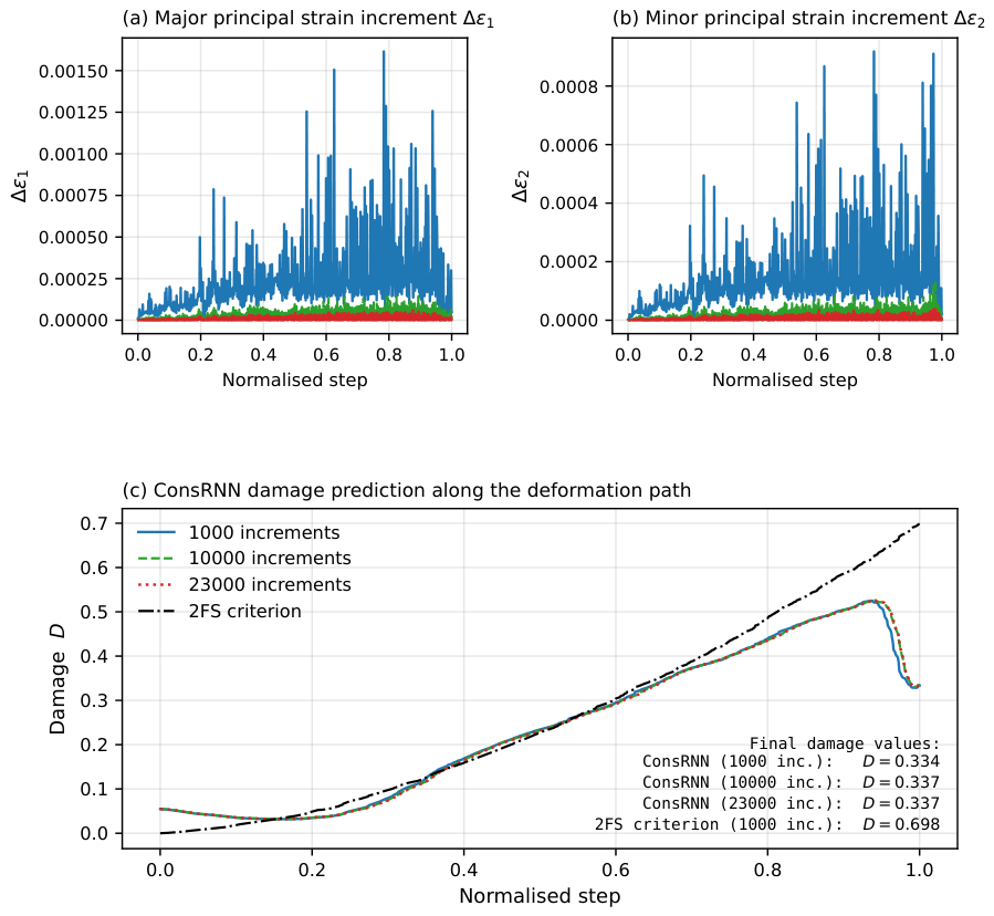
Figure 14.
ConsRNN damage predictions at Element 3089, Integration Point 3, sampled at three temporal resolutions (700, 7000, and 16000 increments): (a) major and (b) minor principal strain increments; (c) damage evolution compared with the 2FS criterion.
Figure 14.
ConsRNN damage predictions at Element 3089, Integration Point 3, sampled at three temporal resolutions (700, 7000, and 16000 increments): (a) major and (b) minor principal strain increments; (c) damage evolution compared with the 2FS criterion.
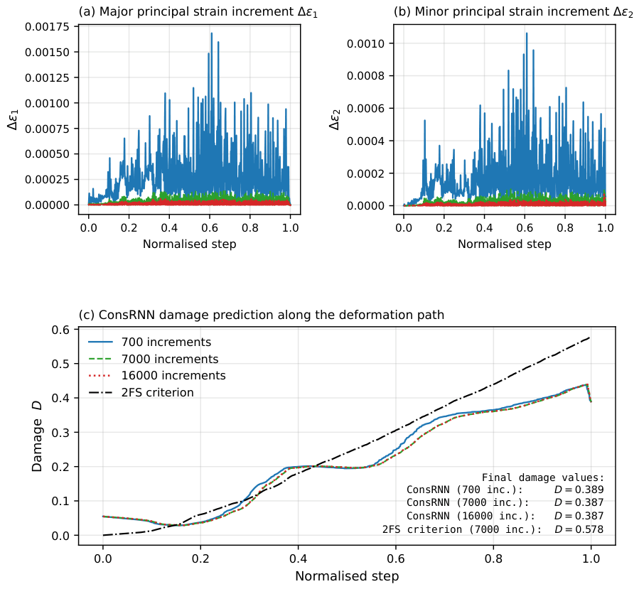
Figure 15.
ConsRNN damage predictions at Element 2750, Integration Point 1, sampled at three temporal resolutions (340, 3400, and 7800 increments): (a) major and (b) minor principal strain increments; (c) damage evolution compared with the 2FS criterion.
Figure 15.
ConsRNN damage predictions at Element 2750, Integration Point 1, sampled at three temporal resolutions (340, 3400, and 7800 increments): (a) major and (b) minor principal strain increments; (c) damage evolution compared with the 2FS criterion.
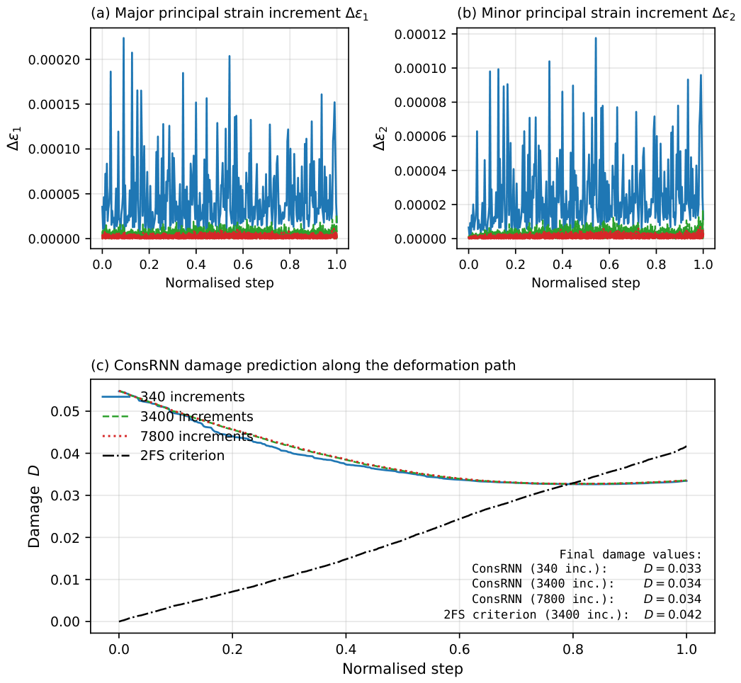
Figure 16.
Global force–displacement response with element erosion governed by the 2FS fracture criterion (dashed) and the embedded ConsRNN surrogate (solid). Both reach the same peak force ( kN) at the same displacement ( mm) and diverge only on the post-peak softening branch. The ConsRNN surrogate operates as a live element-deletion criterion inside the VUMAT.
Figure 16.
Global force–displacement response with element erosion governed by the 2FS fracture criterion (dashed) and the embedded ConsRNN surrogate (solid). Both reach the same peak force ( kN) at the same displacement ( mm) and diverge only on the post-peak softening branch. The ConsRNN surrogate operates as a live element-deletion criterion inside the VUMAT.
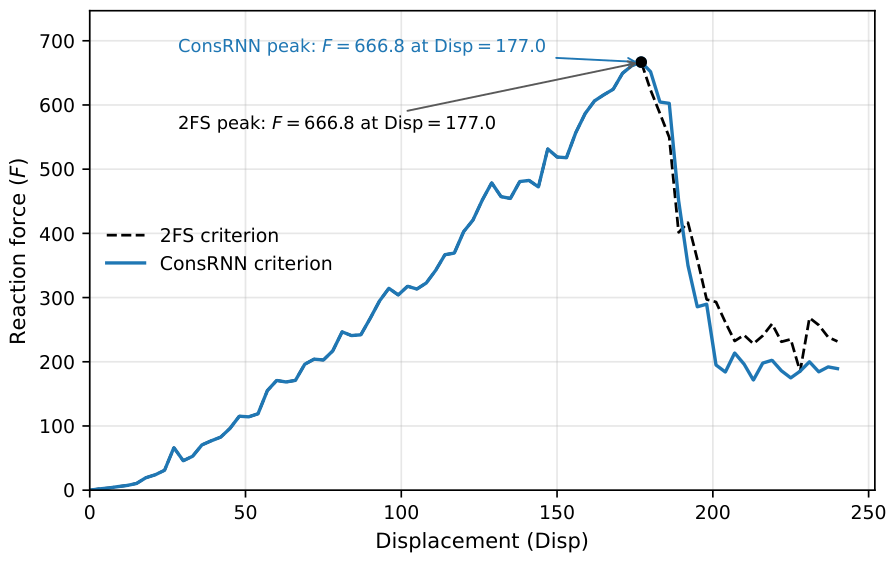

Table 1.
Comparison of ConsRNN and SimpleRNN cells in terms of input transformation, normalisation, and state updates.
Table 1.
Comparison of ConsRNN and SimpleRNN cells in terms of input transformation, normalisation, and state updates.
| Step | ConsRNN | SimpleRNN |
|---|---|---|
| Input | ||
| normalisation | - | |
| Transition | ||
| Update | - | |
| Output |
Table 2.
Test set results for SimpleRNN and ConsRNN on both output scales. Both are the lowest-validation-MSE configurations (batch size 16).
Table 2.
Test set results for SimpleRNN and ConsRNN on both output scales. Both are the lowest-validation-MSE configurations (batch size 16).
| Output Type | Model | RMSE | MAE | nRMSE | MAPE (%) | P95 abs err | |
|---|---|---|---|---|---|---|---|
| Converted Output | SimpleRNN | 0.0281 | 0.0188 | 0.0289 | 6.23 | 0.0586 | 0.9832 |
| ConsRNN | 0.0236 | 0.0150 | 0.0243 | 5.40 | 0.0502 | 0.9882 | |
| Original Damage Output | SimpleRNN | 0.0616 | 0.0378 | 0.0174 | 7.92 | 0.1161 | 0.9784 |
| ConsRNN | 0.0440 | 0.0281 | 0.0124 | 6.71 | 0.0869 | 0.9890 |
Disclaimer/Publisher’s Note: The statements, opinions and data contained in all publications are solely those of the individual author(s) and contributor(s) and not of MDPI and/or the editor(s). MDPI and/or the editor(s) disclaim responsibility for any injury to people or property resulting from any ideas, methods, instructions or products referred to in the content. |
© 2026 by the authors. Licensee MDPI, Basel, Switzerland. This article is an open access article distributed under the terms and conditions of the Creative Commons Attribution (CC BY) license (http://creativecommons.org/licenses/by/4.0/).
Copyright: This open access article is published under a Creative Commons CC BY 4.0 license, which permit the free download, distribution, and reuse, provided that the author and preprint are cited in any reuse.