
Submitted:
28 August 2026
Posted:
31 August 2026
You are already at the latest version
Abstract
This article examines whether global value added is better explained by territorial scale, sectoral specialization, time, or the configuration that emerges when specific sectors are embedded in specific economies. Using the OECD Trade in Value Added (TiVA) 2025 edition for 1995–2022, the study applies a hypothetico-deductive design to a clean panel of individual economies and ISIC section sectors. The empirical strategy combines fixed-effect variance decomposition, transformation robustness, sectoral-share analysis, principal component analysis, cluster validation, concentration indicators, structural-change measures, and external robustness tests using World Bank WDI covariates. The evidence shows that economy, sector, and year effects are all relevant, but the economy-sector configuration carries the strongest explanatory weight. Controls for GDP, population, GDP per capita, and trade openness confirm that observed differences are not reducible to economic size. More demanding economy-sector fixed-effect models also indicate that sectoral composition remains informative after persistent pair-specific heterogeneity and global year shocks are absorbed. The article contributes to global value-chain and structural-transformation research by showing that value-added heterogeneity is primarily territorial-sectoral: it arises from the way sectors are organized within particular economies.
Keywords:
value added
; OECD TiVA
; global value chains
; structural transformation
; sectoral specialization
; principal component analysis
; fixed effects
; economic complexity
; industrial structure
; trade in value added
1. Introduction
Value added provides a direct way to examine where production is generated, retained, and distributed across economies, sectors, and global production networks. In fragmented production systems, gross trade statistics may obscure the location of value creation because intermediate goods and services often cross several borders before reaching final demand. Value-added measures address this limitation by assigning production to the economies and industries where value is generated, rather than to the last border crossed by a good or service.
The OECD Trade in Value Added (TiVA) framework is designed for this measurement problem. Built from inter-country input-output tables, TiVA indicators trace the domestic and foreign value-added content embedded in production and trade flows (OECD, 2021, 2026a, 2026b). The database is therefore well suited for studying global value chains (GVCs), sectoral specialization, territorial asymmetries, and the changing organization of production across economies.
TiVA and related input-output databases have been widely used to examine bilateral production linkages, vertical specialization, export decomposition, domestic value-added shares, and country-specific GVC participation. Less is known about the statistical architecture of value added across a broad economy-sector-year panel. A key unresolved issue is whether territorial differences, sectoral differences, temporal change, and economy-sector configurations operate as separate sources of variation or as interdependent dimensions of the same production structure.
This article addresses that issue through a multi-stage empirical design applied to OECD TiVA data for 1995–2022. The contribution is threefold. First, it decomposes value-added variation across economies, sectors, years, and economy-sector configurations. Second, it tests whether the same pattern holds when value added is expressed as sectoral shares rather than as absolute levels. Third, it introduces external macroeconomic robustness tests using World Bank WDI covariates and economy-sector fixed effects, allowing scale, development, openness, and productive composition to be interpreted separately.
The analysis follows a hypothetico-deductive logic. Expectations are derived from GVC theory, structural transformation, input-output economics, sectoral specialization, and economic complexity. These expectations are then translated into observable hypotheses and evaluated through a transparent sequence of statistical tests. The aim is not to claim causal effects; it is to assess whether the empirical structure of TiVA value added is consistent with a territorial-sectoral interpretation of global value creation.
1.1. Theoretical Background and Hypothesis Development
GVC theory begins from the premise that value creation is unevenly distributed across firms, sectors, and locations. Research on commodity chains, GVC governance, and production fragmentation shows that territorial capabilities, firm organization, institutional context, technological intensity, and chain position shape how value is captured within production networks (Gereffi, 1999; Gereffi et al., 2005; Baldwin, 2016; Antràs, 2020). If this literature is correct, transformed value added should differ systematically across economies because economies do not occupy equivalent positions in global production.
Structural transformation theory provides a second foundation. Development involves the reallocation of production across agriculture, manufacturing, and services, but the timing, direction, and intensity of this process differ across economies and historical periods (Chenery, 1960; Kuznets, 1973; Duarte & Restuccia, 2010; Herrendorf et al., 2014). The implication is straightforward: sectors should differ in their value-added profiles, and those differences should be interpreted in relation to the territorial contexts in which sectors operate.
Input-output and value-added trade research adds a third argument: economy and sector effects are unlikely to be merely additive. The same sector can occupy different positions across economies depending on technology, domestic linkages, reliance on imported inputs, market size, and supply-chain location (Leontief, 1936; Hummels et al., 2001; Johnson & Noguera, 2012; Koopman et al., 2014; Timmer et al., 2014). This leads to the expectation that economy-sector interactions should account for a substantial share of value-added variation.
A final argument comes from economic complexity and GVC resilience. Productive knowledge is unevenly distributed, and economies combine sectors in distinctive ways (Hidalgo et al., 2007; Hidalgo & Hausmann, 2009; Hausmann et al., 2014). At the same time, crises, trade slowdowns, geopolitical tensions, and supply-chain disruptions can alter production patterns without erasing long-standing structural differences (Baldwin & Freeman, 2022; World Bank, 2020). Time should therefore matter, but it is not expected to dominate the deeper territorial-sectoral architecture of value added.
These theoretical premises lead to six testable hypotheses:
H1. Transformed value added differs systematically across economies.
H2. Transformed value added differs systematically across sectors.
H3. Value-added structures changed during 1995–2022, although temporal variation is expected to be smaller than structural economy-sector variation.
H4. Sectoral value-added profiles are conditional on the economy in which sectors are embedded.
H5. Economies form distinct productive profiles when compared through scale-adjusted sectoral shares.
H6. Sectoral-share structures reveal productive heterogeneity beyond absolute economic scale, development level, trade openness, and persistent economy-sector heterogeneity.
The deductive test follows three linked propositions: global production networks allocate value unevenly across economies; structural transformation makes sectors unequal in their value-added roles; and territorial capabilities condition how sectors generate and retain value. The empirical design evaluates these propositions sequentially, moving from variance decomposition to scale-adjusted sectoral profiles, multivariate classification, concentration indicators, structural-change evidence, external WDI covariates, and economy-sector fixed-effect specifications.
2. Materials and Methods
2.1. Research Design
The study uses a quantitative, comparative, and explanatory design grounded in hypothetico-deductive reasoning. Theoretical propositions from GVC theory, structural transformation, input-output economics, and economic complexity are translated into hypotheses H1–H6 and tested through observable empirical implications. Economy, sector, year, and economy-sector effects test H1–H4; PCA and clustering test H5; and sectoral-share and scale-control models test H6.
The analyses were designed to be reproducible in R and Python. The supplementary scripts implement data cleaning, construction of the clean territorial-sectoral sample, IHS transformation, fixed-effect variance decomposition, cluster validation, sectoral-share models, and external WDI robustness tests. Economy-sector fixed-effect models absorb persistent pair-specific heterogeneity and year effects, while clustered standard errors account for repeated observations within economy-sector units.
2.2. Data Source and Sample Construction
The data come from the OECD Trade in Value Added (TiVA) 2025 edition, principal indicators in levels. The analysed indicator is value added (VALU). The raw file contains reference area, activity, counterpart area, unit of measure, frequency, time period, observed value, and unit multiplier. Because the research question concerns cross-economy and cross-sector structure, the empirical design distinguishes the full raw file from a clean analytical sample.
Three samples were constructed. The full sample keeps all valid observations after removing one non-observation row. The clean territorial sample excludes supranational and regional aggregates, including World, G20, OECD, APEC, ASEAN, NAFTA, and EU aggregates. The clean territorial-sectoral sample further excludes aggregate activity groups and retains 20 ISIC section-level sectors. This final sample is used as the main empirical sample because it avoids comparing individual economies with territorial aggregates or disaggregated sectors with broad activity totals.

Table 1.
Sample construction.
| sample | criterion | observations | economies | sectors | years |
|---|---|---|---|---|---|
| Raw file after removing one non-observation row | Valid observed value and time period | 198958 | 99 | 72 | 28 |
| Clean territorial sample | Excludes supranational/reference-area aggregates; all activity codes retained | 161186 | 80 | 72 | 28 |
| Clean territorial-sectoral sample | Excludes supranational aggregates and retains only 20 ISIC section sectors | 44800 | 80 | 20 | 28 |
Note: The clean territorial-sectoral sample is used as the main empirical sample. Supranational reference-area aggregates and aggregate activity groups are retained only for descriptive benchmarking or supplementary checks.
2.3. Variables and Transformations
The dependent variable is observed value added, reported in the original file as OBS_VALUE. Because the distribution is highly asymmetric and includes negative, zero, and positive observations, the primary models use the inverse hyperbolic sine (IHS) transformation. The IHS transformation behaves similarly to a logarithm for large positive values while retaining zero and negative observations, which makes it appropriate for this type of macroeconomic series.
The transformed outcome is y = asinh(x), where x denotes observed value added and y denotes the transformed value used in the variance-decomposition models. To address scale effects, a second family of models uses sectoral shares: the value added of sector a in economy i and year t divided by total value added across the 20 clean sectors in the same economy-year. These share-based models shift the focus from absolute economic size to productive composition.
The main explanatory dimensions are economy, sector, year, and economy-sector pair. Economy corresponds to the individual reference area after aggregate categories are excluded. Sector corresponds to ISIC section-level activity codes A to T. Year covers 1995–2022.
2.4. Empirical Strategy and Deductive Testing Sequence
The empirical strategy proceeds in four steps. First, fixed-effect variance-decomposition models evaluate whether the theoretical dimensions identified in H1–H4 have measurable counterparts in the data. The null model is compared with economy fixed effects, sector fixed effects, year fixed effects, an additive economy-sector-year model, and a model with economy-sector pair effects plus year effects.
The additive model is written as yᵢₐₜ = μ + αᵢ + βₐ + γₜ + εᵢₐₜ, where yᵢₐₜ is transformed value added for economy i, sector a, and year t; μ is the overall mean; αᵢ is the economy effect; βₐ is the sector effect; γₜ is the year effect; and εᵢₐₜ is the residual term. The interaction model adds θᵢₐ, the economy-sector effect, to capture persistent heterogeneity specific to each economy-sector pair.
Partial F-tests evaluate the incremental contribution of economy, sector, year, and economy-sector effects. Because the sample is large, interpretation emphasizes R², adjusted R², incremental R², and partial eta squared rather than p-values alone. This avoids treating statistical significance as sufficient evidence of substantive relevance.
Second, the analysis examines scale-adjusted productive structure. Mean sectoral shares are organized as an economy-by-sector matrix. PCA identifies latent dimensions of sectoral composition (Jolliffe, 2002; Jolliffe & Cadima, 2016). K-means clustering is then applied to standardized sectoral-share profiles, with validation through silhouette, Calinski–Harabasz, Davies–Bouldin, and subperiod stability statistics.
Third, the study measures concentration and structural change. Sectoral concentration is calculated with the Herfindahl-Hirschman Index, HHI = Σs², where s is the sectoral share. Structural change between 1995 and 2022 is measured as one-half of the sum of absolute differences in sectoral shares across the two endpoints.
Fourth, the paper adds scale-control and composition robustness. Because value-added levels are mechanically related to economic scale, the robustness models include a production-side economy-year scale control, sectoral shares, HHI, World Bank WDI covariates, and economy-sector fixed effects. This sequence separates absolute scale from productive composition and tests whether the central claim remains after persistent economy-sector heterogeneity is absorbed.
3. Results
3.1. Dataset Structure and Clean-Sample Descriptives
The clean territorial-sectoral sample contains 44,800 observations: 80 individual economies, 20 ISIC section sectors, and 28 annual periods. Observed value added remains highly dispersed after aggregate categories are excluded, with maximum values far above the median. This dispersion confirms that transformation and scale-adjusted checks are necessary before substantive interpretation.
Table 2.
Descriptive structure of the clean territorial-sectoral sample.
| statistic | value |
|---|---|
| Observations | 44800 |
| Economies | 80 |
| ISIC section sectors | 20 |
| Years | 1995–2022 |
| Minimum observed value | -1661 |
| Median observed value | 3,552,314.50 |
| Mean observed value | 31,523,733.09 |
| SD observed value | 134,793,127.03 |
| Maximum observed value | 4966806447 |
Note: Observed values are taken directly from the supplied TiVA file. The analytical models use the inverse hyperbolic sine transformation of observed value added.
3.2. Fixed-Effect Variance Decomposition
Table 3 reports the fixed-effect variance-decomposition models. Economy fixed effects explain 45.4% of the variance in transformed value added, sector fixed effects explain 20.4%, and year fixed effects explain 3.7%. The additive economy-sector-year model explains 69.5% of the variance. The economy-sector plus year model raises the explained variance to 90.4%, indicating that value-added heterogeneity is organized mainly through the pairing of economies and sectors.
The partial F-tests in Table 4 confirm that each theoretical dimension has empirical support, although the magnitudes differ. The economy effect has a partial eta squared of 0.598, the sector effect 0.401, and the year effect 0.108. The economy-sector interaction reaches a partial eta squared of 0.685, reinforcing the interpretation that sectoral value added depends strongly on the territorial context in which sectors are embedded.
3.3. Transformation Robustness
The main conclusions remain stable under alternative transformations. The interaction model outperforms the additive model under IHS, shifted-log, and winsorized-IHS transformations. Although the incremental R² changes across transformations, the substantive pattern is consistent: economy-sector structure explains more than additive economy, sector, and year effects alone.
Table 5.
Transformation robustness.
| transformation | additive_r2 | interaction_r2 | incremental_r2 | rmse_interaction |
|---|---|---|---|---|
| Inverse hyperbolic sine | 0.695 | 0.904 | 0.209 | 0.857 |
| Shifted log | 0.774 | 0.889 | 0.115 | 0.827 |
| Winsorized IHS | 0.765 | 0.888 | 0.122 | 0.842 |
Note: Shifted log uses a constant sufficient to make all observations positive. Winsorized IHS clips the observed value at the 1st and 99th percentiles before applying the IHS transformation.
3.4. Internal Scale-Control and Sectoral-Share Robustness
Table 6 addresses the most direct scale-related concern: larger economies naturally generate larger absolute value added. After sector and year effects are included, the economy-year scale control increases adjusted R² from 0.241 to 0.693. Adding sectoral share and HHI further improves model fit. These results show that scale matters, but they also show that composition and concentration add information beyond scale.
Table 6b provides the complementary size-free test. When sectoral share is used as the dependent variable, the economy-year scale coefficient is essentially zero and statistically non-significant across specifications. This result is central to H6: productive composition remains empirically distinct from absolute economic size.
3.5. External Macroeconomic Robustness with World Bank WDI Covariates
To test whether the results merely reflect economy size or development level, the clean TiVA panel was merged with World Bank World Development Indicators for GDP, population, GDP per capita, and trade openness. The merge retained 42,180 observations, covering 77 economies, 20 ISIC sectors, and 28 years. Myanmar, Nigeria, and Taiwan were not retained in the complete-case panel because at least one required WDI variable was unavailable.
Table 6c reports the external robustness models. Adding GDP to the baseline sector-year model raises adjusted R² from 0.245 to 0.684, confirming that macroeconomic scale is relevant for absolute value-added levels. Yet scale does not exhaust the structure. When population, GDP per capita, trade openness, sectoral share, HHI, and fixed effects are included, the models continue to identify a distinct role for sectoral composition.
Table 6d reports selected coefficients from the external robustness specifications. In the scale-development-composition model, log population and log GDP per capita remain positive and statistically significant. Sectoral share is also positive and significant, while HHI is negative and significant. These estimates suggest that value-added levels are shaped by macroeconomic scale and by the internal organization of production.
3.5.1. Economy-Sector Fixed-Effect Robustness
The WDI robustness tests were extended with economy-sector fixed effects. This is the most demanding specification in the article because it absorbs persistent heterogeneity specific to each economy-sector pair and identifies the remaining association from within-pair changes over time, net of year effects. The purpose is not to replace the descriptive and multivariate evidence, but to test whether the composition result survives a stricter longitudinal specification.
Table 6e shows that WDI controls alone explain a modest share of within economy-sector variation once pair effects and year effects are absorbed. When sectoral share and HHI are added, the adjusted within R² rises from 0.073 to 0.437. This pattern is important because it shows that sectoral composition remains informative even after long-standing economy-sector differences are controlled.
Table 6f reports selected coefficients from the economy-sector fixed-effect models. Log population and log GDP per capita remain positive and statistically significant in the IHS value-added specifications. In M9, sectoral share is positive and significant, while HHI is negative and significant. The evidence therefore supports H6 under the strictest specification used in the study.
3.6. Sectoral Profiles and Scale-Adjusted Composition
Absolute levels identify the sectors that generate the largest amounts of value added in the clean sample, including manufacturing, wholesale and retail trade, real estate, public administration, finance, and construction. Because absolute levels remain affected by economy size, the share-based analysis is interpreted as the main evidence on productive structure.
Table 7.
Top ten ISIC section sectors by mean observed value added.
| ACTIVITY | sector_label | n | mean_observed_value | mean_share | mean_ihs |
|---|---|---|---|---|---|
| C | Manufacturing | 2240 | 112,274,678.93 | 0.171 | 17.341 |
| G | Wholesale and retail trade; repair of motor vehicles | 2240 | 75,130,415.95 | 0.121 | 17.050 |
| L | Real estate activities | 2240 | 61,146,561.08 | 0.078 | 16.513 |
| O | Public administration and defence; compulsory social security | 2240 | 40,917,862.98 | 0.062 | 16.339 |
| K | Financial and insurance activities | 2240 | 38,922,699.53 | 0.054 | 16.137 |
| F | Construction | 2240 | 35,793,272.19 | 0.057 | 16.247 |
| Q | Human health and social work activities | 2240 | 34,390,215.41 | 0.040 | 15.747 |
| M | Professional, scientific and technical activities | 2240 | 33,346,696.57 | 0.039 | 15.740 |
| J | Information and communication | 2240 | 30,388,991.77 | 0.042 | 15.981 |
| P | Education | 2240 | 29,902,084.31 | 0.044 | 16.004 |
Note: The table reports clean-sample sector profiles. Sectoral shares are calculated within each economy-year across the 20 ISIC section sectors.
3.7. PCA of Sectoral Value-Added Shares
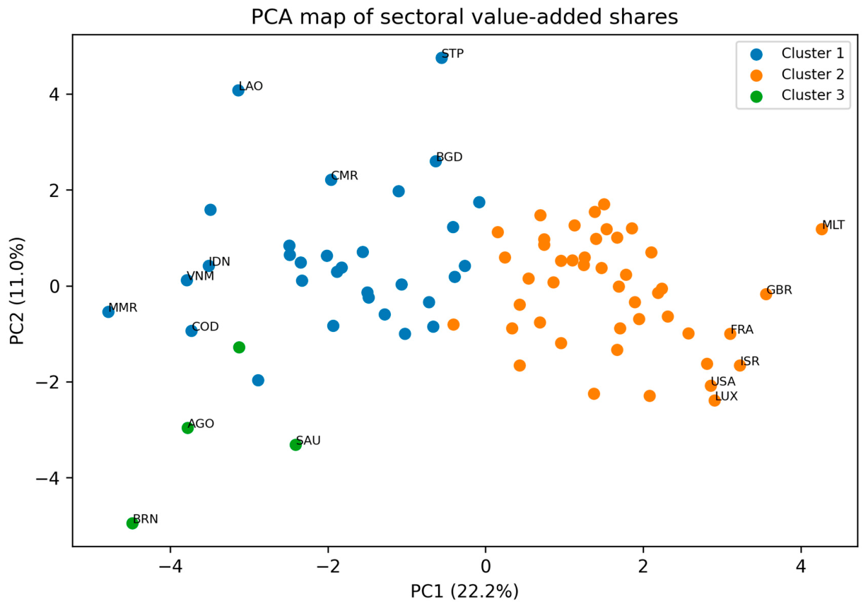
The PCA of sectoral shares identifies latent dimensions of productive structure. The first six principal components explain 64.7% of standardized sectoral-share variance. PC1 explains 22.2% and PC2 explains 11.0%. The distribution of variance across several components indicates that productive structure is multidimensional rather than reducible to a single sectoral axis.
Table 8.
PCA explained variance.
| component | eigenvalue | explained_variance | cumulative_variance |
|---|---|---|---|
| PC1 | 4.490 | 0.222 | 0.222 |
| PC2 | 2.236 | 0.110 | 0.332 |
| PC3 | 1.862 | 0.092 | 0.424 |
| PC4 | 1.735 | 0.086 | 0.510 |
| PC5 | 1.397 | 0.069 | 0.579 |
| PC6 | 1.382 | 0.068 | 0.647 |
| PC7 | 1.020 | 0.050 | 0.697 |
| PC8 | 0.959 | 0.047 | 0.745 |
Note: PCA was estimated on standardized mean sectoral shares for 80 economies and 20 ISIC section sectors.
Figure 1.
PCA scree plot for sectoral value-added shares.
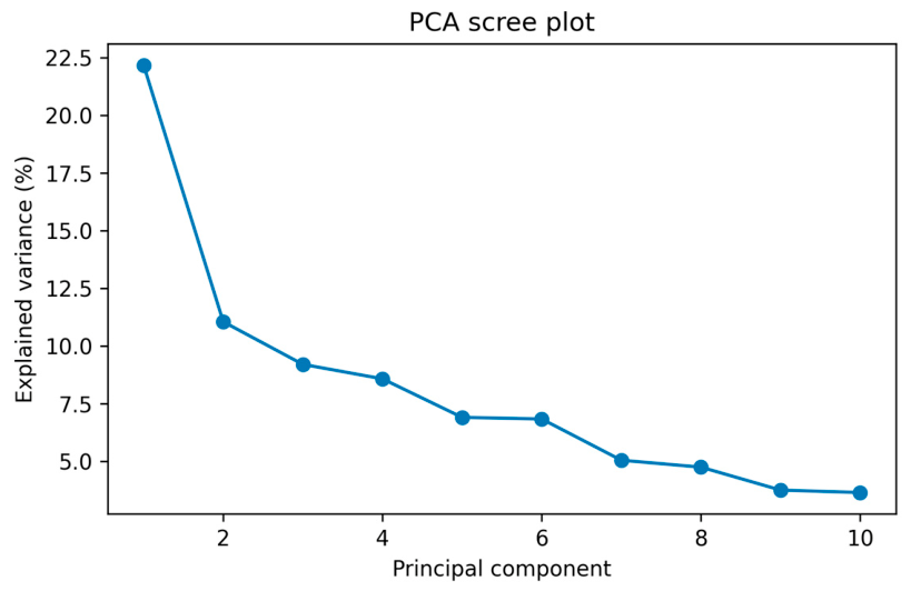
Figure 2.
Economies in the PCA space of sectoral value-added shares.
3.8. Clustering and Productive Profiles
Cluster validation suggests that economy profiles are heterogeneous rather than sharply separated into a single natural partition. The k = 4 solution produces the highest silhouette score among the tested alternatives, whereas the k = 3 solution offers a more parsimonious and interpretable classification. For that reason, the three-cluster solution is used in the main text, and the validation metrics are reported transparently.
Table 9.
Cluster validation metrics.
| k | within_cluster_ss | silhouette | calinski_harabasz | davies_bouldin |
|---|---|---|---|---|
| 2.000 | 1,337.06 | 0.167 | 15.339 | 2.103 |
| 3.000 | 1,227.99 | 0.171 | 11.663 | 1.817 |
| 4.000 | 1,129.82 | 0.183 | 10.543 | 1.430 |
| 5.000 | 1,054.91 | 0.103 | 9.689 | 1.731 |
| 6.000 | 979.565 | 0.100 | 9.374 | 1.483 |
| 7.000 | 914.200 | 0.093 | 9.127 | 1.435 |
| 8.000 | 869.622 | 0.090 | 8.639 | 1.473 |
Note: K-means clustering was estimated on standardized sectoral-share profiles. Higher silhouette and Calinski–Harabasz values indicate better separation; lower Davies–Bouldin values indicate better compactness and separation.
The three-cluster solution separates economies with relatively manufacturing-agricultural profiles, diversified service-intensive profiles, and strongly extractive profiles. The extractive cluster is small and includes Angola, the United Arab Emirates, Brunei, and Saudi Arabia, reflecting high average shares in mining and quarrying. The service-intensive and manufacturing-agricultural clusters are broader and should be read as structural tendencies rather than rigid categories.
Figure 3.
Heatmap of economy-sector value-added shares.
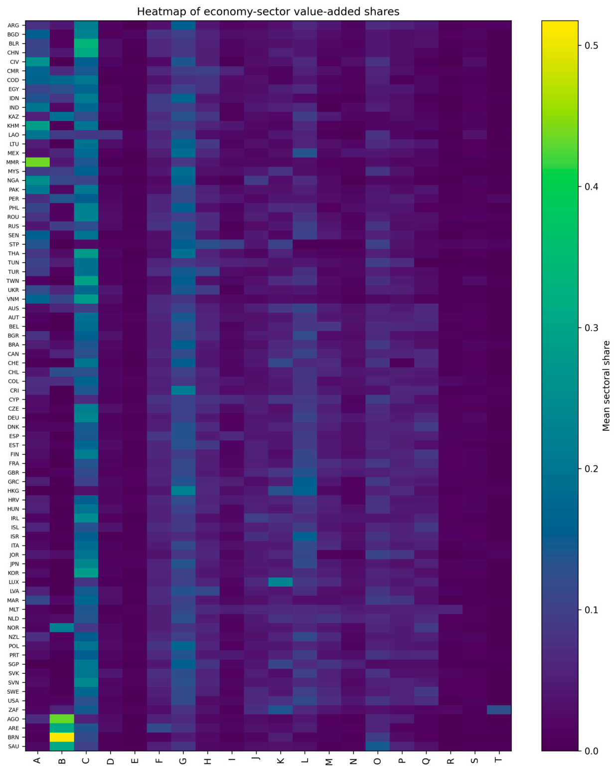
Table 10.
Cluster centroids by sectoral share.
| sector | sector_label | Cluster 1 | Cluster 2 | Cluster 3 |
|---|---|---|---|---|
| A | Agriculture, forestry and fishing | 0.139 | 0.032 | 0.029 |
| B | Mining and quarrying | 0.058 | 0.021 | 0.391 |
| C | Manufacturing | 0.191 | 0.162 | 0.103 |
| D | Electricity, gas, steam and air conditioning supply | 0.020 | 0.021 | 0.018 |
| E | Water supply; sewerage and waste management | 0.006 | 0.009 | 0.003 |
| F | Construction | 0.056 | 0.058 | 0.060 |
| G | Wholesale and retail trade; repair of motor vehicles | 0.129 | 0.120 | 0.069 |
| H | Transportation and storage | 0.062 | 0.056 | 0.026 |
| I | Accommodation and food service activities | 0.027 | 0.026 | 0.015 |
| J | Information and communication | 0.035 | 0.048 | 0.029 |
| K | Financial and insurance activities | 0.041 | 0.064 | 0.035 |
| L | Real estate activities | 0.059 | 0.095 | 0.036 |
Note: Centroids are expressed in original sectoral-share units. Only the first 12 sectors are shown in the main text; the complete table is provided as supplementary material.
3.8.1. Cluster Stability Across Subperiods
Because clustering is used as typological evidence rather than as a causal estimator, the stability of the classification was evaluated across subperiods. The comparison covers early-period profiles (1995–2008), recent-period profiles (2009–2022), and the full-period classification. The purpose is to assess whether the groups reflect persistent productive structure or a short-run pattern.
Table 10.
b. Cluster validation across subperiods.
| Period | k | Silhouette | Calinski–Harabasz | Davies–Bouldin | Within-cluster SS |
|---|---|---|---|---|---|
| 1995–2008 | 3 | 0.184 | 12.054 | 1.775 | 1218.509 |
| 1995–2008 | 4 | 0.187 | 10.714 | 1.320 | 1124.434 |
| 2009–2022 | 3 | 0.160 | 11.020 | 1.928 | 1243.935 |
| 2009–2022 | 4 | 0.181 | 9.917 | 1.514 | 1149.865 |
| 1995–2022 | 3 | 0.170 | 11.219 | 1.732 | 1238.969 |
| 1995–2022 | 4 | 0.169 | 10.167 | 1.792 | 1141.787 |
Table 10.
c. Cluster stability based on Adjusted Rand Index.
| Comparison | Adjusted Rand Index | Interpretation |
|---|---|---|
| 1995–2008 vs 2009–2022 | 0.679 | Typologies display moderate persistence and meaningful structural reallocation across subperiods. |
| 1995–2022 vs 2009–2022 | 0.699 | The full-period classification is close to the recent-period structure, supporting use as a long-run typology. |
Note: Adjusted Rand Index values closer to 1 indicate stronger agreement between two classifications. The observed values indicate moderate persistence, which is appropriate for a long-run structural typology: economies do not reshuffle randomly across profiles, although some reallocation occurs between subperiods.
3.9. Sectoral Concentration and Structural Change
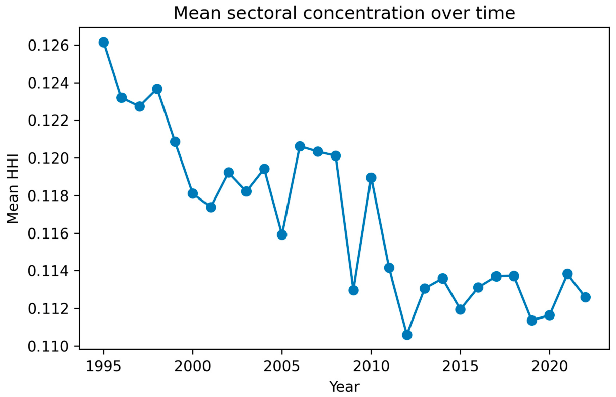
The HHI results show that sectoral concentration varies considerably across economies. Brunei, Myanmar, Angola, Cambodia, Saudi Arabia, Belarus, Viet Nam, the United Arab Emirates, Thailand, and China show the highest average concentration in the clean sample. Concentration is therefore not limited to oil-based economies; it may also reflect specialization in manufacturing, agriculture, or trade-related structures.
Table 11.
Top ten economies by average sectoral concentration.
| REF_AREA | mean_hhi | min_hhi | max_hhi | sd_hhi |
|---|---|---|---|---|
| BRN | 0.314 | 0.147 | 0.372 | 0.042 |
| MMR | 0.245 | 0.085 | 0.361 | 0.055 |
| AGO | 0.228 | 0.079 | 0.298 | 0.052 |
| KHM | 0.174 | 0.086 | 0.294 | 0.042 |
| SAU | 0.169 | 0.096 | 0.235 | 0.038 |
| BLR | 0.163 | 0.077 | 0.223 | 0.030 |
| VNM | 0.163 | 0.096 | 0.245 | 0.034 |
| ARE | 0.158 | 0.094 | 0.201 | 0.028 |
| THA | 0.154 | 0.120 | 0.191 | 0.015 |
| CHN | 0.154 | 0.075 | 0.224 | 0.033 |
Note: HHI is computed from sectoral value-added shares across the 20 ISIC section sectors for each economy-year.
Figure 4.
Mean sectoral concentration over time.
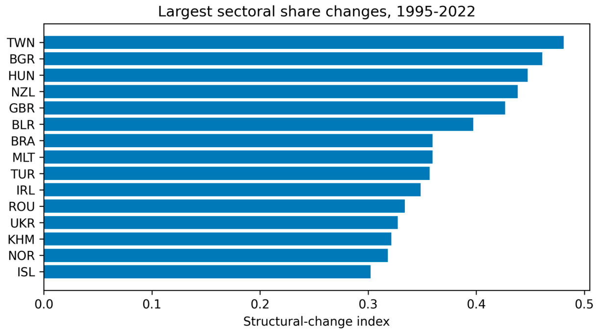
The structural-change index identifies the economies with the largest sectoral-share shifts between 1995 and 2022. Taiwan, Bulgaria, Hungary, New Zealand, the United Kingdom, Belarus, Brazil, Malta, Turkiye, and Ireland show the largest shifts. This result supports H3 in a qualified sense: time matters, but the observed changes occur within persistent territorial-sectoral structures rather than as a common global time trend.
Table 12.
Top ten structural-change indices, 1995–2022.
| REF_AREA | structural_change_index |
|---|---|
| TWN | 0.481 |
| BGR | 0.461 |
| HUN | 0.447 |
| NZL | 0.438 |
| GBR | 0.427 |
| BLR | 0.397 |
| BRA | 0.360 |
| MLT | 0.360 |
| TUR | 0.357 |
| IRL | 0.349 |
Note: The structural-change index equals one-half of the sum of absolute differences in sectoral shares between 1995 and 2022.
Figure 5.
Largest sectoral share changes, 1995–2022.
3.10. Hypothesis Testing Summary
Table 13 closes the deductive loop between theory and evidence. H1, H2, H4, H5, and H6 are supported. H3 is partially supported: year effects are statistically significant and structural change is observable, but temporal effects explain less variance than territorial-sectoral structure. Overall, the evidence is most consistent with the article’s central expectation that global value-added heterogeneity is organized through economy-sector configurations.
4. Discussion
4.1. Territorial Asymmetries in Value-Added Formation
The evidence supports H1. Economy fixed effects account for a substantial share of transformed value-added variance, which is consistent with GVC and input-output research showing that economies capture value from global production networks unevenly (Johnson & Noguera, 2012; Koopman et al., 2014; Timmer et al., 2014). This should not be read as a causal effect of geography. Economy-level differences summarize persistent variation in scale, capabilities, institutions, domestic linkages, and positions within production networks.
The policy implication is clear: participation in global trade does not automatically lead to value-added upgrading. An economy may be highly connected to global production while retaining limited domestic value added if it specializes in lower-value segments or depends heavily on imported intermediates (Baldwin, 2016; Gereffi, 2018; World Bank, 2020).
4.2. Sectoral Specialization and Productive Structure
H2 is also supported. Sector fixed effects and sectoral profiles show that value-added formation differs markedly across activities. Manufacturing, wholesale and retail trade, real estate, public administration, finance, and construction occupy major positions in absolute levels, while share-based analysis shows that internal productive composition differs across economies. This is consistent with structural transformation theory, in which growth is associated with changes in the organization of production across sectors rather than with uniform expansion across all activities.
The sectoral result also cautions against treating manufacturing or services as homogeneous categories. Even at the ISIC section level, TiVA data reveal substantial heterogeneity. More disaggregated industry data would likely expose additional structure within manufacturing, business services, digital activities, and resource-based sectors.
4.3. Time Matters, but Structure Matters More
H3 receives qualified support. Year effects are statistically significant, and the structural-change index shows that many economies altered their sectoral shares between 1995 and 2022. Nevertheless, year effects explain less variance than economy, sector, and economy-sector effects. Temporal change is therefore observable, but it appears to operate through pre-existing territorial-sectoral structures rather than replacing them.
4.4. The Economy-Sector Interaction as the Core Finding
H4 is the main empirical contribution of the article. The economy-sector plus year model explains 90.4% of transformed value-added variance, far above the additive economy-sector-year model. Sectoral value added is therefore not a property of sectors alone. A sector’s contribution depends on the economy in which it operates, reflecting differences in productive capabilities, domestic linkages, technology, market size, and GVC position. The finding connects GVC theory and structural transformation theory by showing that production networks allocate activities across territories, while territories give those activities different value-added profiles.
4.5. Multivariate Productive Profiles and Scale-Adjusted Structure
H5 and H6 are supported by the multivariate and external robustness evidence. PCA shows that sectoral-share profiles are multidimensional, while clustering identifies interpretable productive profiles with moderate subperiod stability. The extractive cluster is small but clearly distinct; diversified service-intensive and manufacturing-agricultural profiles are broader and more heterogeneous. The WDI and economy-sector fixed-effect models further show that scale and development controls do not eliminate the relevance of sectoral composition. This strengthens the claim that value-added structures reflect productive configurations, not only economy size.
4.6. External Macroeconomic Robustness and the Interpretation of Scale
The external WDI robustness tests sharpen the interpretation of absolute value-added levels. GDP, population, and GDP per capita are not nuisance variables; they describe the macroeconomic scale and development conditions under which sectors generate value added. The models confirm an expected result: larger and more developed economies tend to report higher absolute value added. This does not weaken the argument; it clarifies which part of the evidence concerns scale and which part concerns sectoral structure.
More importantly, the robustness models show that scale is not the whole story. After WDI covariates, sectoral shares, HHI, economy-sector fixed effects, and year effects are introduced, the evidence still points to a territorial-sectoral structure. Sectoral share remains strongly associated with transformed value added in the demanding economy-sector specification, while sectoral concentration is negatively associated with it. Economies therefore differ not only because they are large or small, but also because value added is organized through different sectoral configurations that evolve within persistent economy-sector structures.
4.7. Limitations and Future Research
Several limitations should be noted. First, the analysis identifies structural associations rather than causal effects. Second, value-added levels are sensitive to economy size, although this concern is addressed through sectoral shares, internal scale controls, external WDI covariates, and economy-sector fixed effects. Third, the WDI robustness exercise is based on a complete-case merge; three economies in the clean TiVA panel could not be retained because at least one required external indicator was unavailable. Fourth, the study uses current US-dollar TiVA levels; size-free shares and WDI controls mitigate this issue but do not fully replace a constant-price value-added series. Fifth, TiVA indicators are derived from inter-country input-output tables and therefore inherit the assumptions and revisions of that accounting framework. Finally, ISIC sections simplify the diversity of activities within each sector.
Future research can extend this design by combining TiVA levels and official TiVA shares with richer country-year covariates, including productivity, human capital, institutional quality, innovation intensity, foreign direct investment, exchange-rate indicators, and constant-price value-added measures. These extensions would allow researchers to move from structural diagnosis toward more explicit explanations of why some economies upgrade into higher value-added configurations while others remain concentrated in narrower productive profiles.
5. Conclusions
This article examined territorial-sectoral heterogeneity in global value added using OECD TiVA data for 1995–2022. The empirical design combines fixed-effect variance decomposition, partial F-tests, sectoral shares, PCA, clustering, HHI, structural-change indices, transformation robustness checks, external WDI covariates, and economy-sector fixed effects. The main clean sample contains 44,800 observations for 80 economies, 20 ISIC section sectors, and 28 years.
The central conclusion is direct: value-added heterogeneity is territorial-sectoral. Economy and sector effects matter separately, but their interaction explains more. The economy-sector plus year model accounts for 90.4% of transformed value-added variance, indicating that global value creation cannot be understood adequately through isolated country rankings or sector rankings. It is shaped by the way specific sectors are embedded in specific economies.
The share-based, scale-control, and WDI robustness analyses reinforce this conclusion. Absolute value added is partly a function of economy-year size, but productive composition is not reducible to that scale. PCA, clustering, HHI, and structural-change indicators further show that economies differ by configuration, concentration, and transformation trajectory. The article therefore offers a structural diagnostic framework for analysing how economies generate value added within global production networks.
Supplementary Materials
The following supporting information can be downloaded at the website of this paper posted on Preprints.org. The supplementary package submitted with this article includes: Table S1: full clean-sample descriptive statistics; Table S2: fixed-effect model outputs; Table S3: partial F-tests; Table S4: transformation robustness; Table S5: internal scale-control models; Table S6: sectoral-share robustness models; Table S7: WDI external robustness outputs; Table S8: economy-sector fixed-effect robustness outputs; Table S9: PCA loadings; Table S10: cluster validation and stability metrics; Table S11: HHI and structural-change rankings; Script S1: full replication script; Data S1: clean TiVA-WDI analytical panel.
Author Contributions
Conceptualization, A.-R.G.-P.; methodology, A.-R.G.-P.; software, A.-R.G.-P.; validation, A.-R.G.-P.; formal analysis, A.-R.G.-P.; investigation, A.-R.G.-P.; resources, A.-R.G.-P.; data curation, A.-R.G.-P.; writing—original draft preparation, A.-R.G.-P.; writing—review and editing, A.-R.G.-P.; visualization, A.-R.G.-P.; supervision, A.-R.G.-P.; project administration, A.-R.G.-P. The author has read and agreed to the published version of the manuscript.
Funding
This research received no external funding.
Institutional Review Board Statement
Not applicable.
Informed Consent Statement
Not applicable.
Data Availability Statement
The TiVA data analysed in this study are publicly available from the OECD Trade in Value Added database, 2025 edition. The external macroeconomic covariates are publicly available from the World Bank World Development Indicators. Processed analytical tables, the clean TiVA-WDI merged panel, cluster-stability outputs, economy-sector fixed-effect outputs, and reproducible scripts are provided as supplementary materials or are available from the corresponding author upon reasonable request.
Acknowledgments
The author acknowledges the OECD for providing public access to the Trade in Value Added database and the World Bank for providing public access to the World Development Indicators. AI-assisted tools were used only for language editing, structure checking, and formatting support. The author reviewed and edited all outputs and takes full responsibility for the content of this publication.
Conflicts of Interest
The author declares no conflicts of interest.
Abbreviations
| Abbreviation | Meaning |
| ANOVA | Analysis of variance |
| APEC | Asia-Pacific Economic Cooperation |
| FE | Fixed effects |
| G20 | Group of Twenty |
| GVC | Global value chain |
| HHI | Herfindahl-Hirschman Index |
| ICIO | Inter-Country Input-Output |
| IHS | Inverse hyperbolic sine |
| ISIC | International Standard Industrial Classification |
| OECD | Organisation for Economic Co-operation and Development |
| PCA | Principal component analysis |
| TiVA | Trade in Value Added |
| USD | United States dollar |
Appendix A. Reproducibility and Model Details
The core transformation is y = asinh(x), where x is observed value added. Sectoral shares are computed as sᵢₐₜ = xᵢₐₜ / Σₐxᵢₐₜ for economy i, sector a, and year t. The HHI is computed as HHIᵢₜ = Σₐsᵢₐₜ². The structural-change index is SCIᵢ = 0.5Σₐ|sᵢₐ,2022 - sᵢₐ,1995|. PCA and clustering use standardized mean sectoral shares. The fixed-effect models compare null, economy, sector, year, additive, and economy-sector specifications. This appendix documents the theoretical-to-empirical sequence used to make the analysis transparent and reproducible.
References
- Amador; Cabral; Amador, J.; Cabral, S. Global value chains: A survey of drivers and measures. Journal of Economic Surveys 2016, 30(2), 278–301. [Google Scholar] [CrossRef]
- Antràs; Antràs, P. Conceptual aspects of global value chains. World Bank Economic Review 2020, 34(3), 551–574. [Google Scholar] [CrossRef]
- Antràs; Chor; Antràs, P.; Chor, D. Organizing the global value chain. Econometrica 2013, 81(6), 2127–2204. [Google Scholar] [CrossRef]
- Baldwin; Baldwin, R. Trade and industrialisation after globalisation’s second unbundling: How building and joining a supply chain are different and why it matters; NBER Working Paper No. 17716; 2011. [Google Scholar] [CrossRef]
- Baldwin; Baldwin, R. The great convergence: Information technology and the new globalization; Harvard University Press, 2016. [Google Scholar]
- Baldwin; Freeman; Baldwin, R.; Freeman, R. Risks and global supply chains: What we know and what we need to know. Annual Review of Economics 2022, 14, 153–180. [Google Scholar] [CrossRef]
- Baldwin; Venables; Baldwin, R.; Venables, A. J. Spiders and snakes: Offshoring and agglomeration in the global economy. Journal of International Economics 2013, 90(2), 245–254. [Google Scholar] [CrossRef]
- Bellemare; Wichman; Bellemare, M. F.; Wichman, C. J. Elasticities and the inverse hyperbolic sine transformation. Oxford Bulletin of Economics and Statistics 2020, 82(1), 50–61. [Google Scholar] [CrossRef]
- Burbidge; Burbidge, J. B.; Magee, L.; Robb, A. L. Alternative transformations to handle extreme values of the dependent variable. Journal of the American Statistical Association 1988, 83(401), 123–127. [Google Scholar] [CrossRef]
- Chenery; Chenery, H. B. Patterns of industrial growth. American Economic Review 1960, 50(4), 624–654. [Google Scholar]
- Chenery & Taylor; Chenery, H. B.; Taylor, L. Development patterns: Among countries and over time. Review of Economics and Statistics 1968, 50(4), 391–416. [Google Scholar] [CrossRef] [PubMed]
- Costinot; Costinot, A.; Vogel, J.; Wang, S. An elementary theory of global supply chains. Review of Economic Studies 2013, 80(1), 109–144. [Google Scholar] [CrossRef]
- Cristelli; Cristelli, M.; Gabrielli, A.; Tacchella, A.; Caldarelli, G.; Pietronero, L. Measuring the intangibles: A metrics for the economic complexity of countries and products. PLoS ONE 2013, 8(8), e70726. [Google Scholar] [CrossRef] [PubMed]
- Daudin; Daudin, G.; Rifflart, C.; Schweisguth, D. Who produces for whom in the world economy? Canadian Journal of Economics 2011, 44(4), 1403–1437. [Google Scholar] [CrossRef]
- de Backer; Miroudot; de Backer, K.; Miroudot, S. Mapping global value chains; OECD Trade Policy Papers, No. 159; 2013. [Google Scholar] [CrossRef]
- Dietzenbacher; Dietzenbacher, E.; Los, B.; Stehrer, R.; Timmer, M. P.; de Vries, G. J. The construction of world input-output tables in the WIOD project. Economic Systems Research 2013, 25(1), 71–98. [Google Scholar] [CrossRef]
- Duarte; Restuccia; Duarte, M.; Restuccia, D. The role of the structural transformation in aggregate productivity. Quarterly Journal of Economics 2010, 125(1), 129–173. [Google Scholar] [CrossRef]
- Everitt; Everitt, B. S.; Landau, S.; Leese, M.; Stahl, D. Cluster analysis, 5th ed.; Wiley, 2011. [Google Scholar]
- Feenstra; Feenstra, R. C. Integration of trade and disintegration of production in the global economy. Journal of Economic Perspectives 1998, 12(4), 31–50. [Google Scholar] [CrossRef]
- Feenstra; Hanson; Feenstra, R. C.; Hanson, G. H. Globalization, outsourcing, and wage inequality. American Economic Review 1996, 86(2), 240–245. [Google Scholar]
- Fox; Weisberg; Fox, J.; Weisberg, S. An R companion to applied regression, 3rd ed.; Sage, 2019. [Google Scholar]
- Gereffi; Gereffi, G. International trade and industrial upgrading in the apparel commodity chain. Journal of International Economics 1999, 48(1), 37–70. [Google Scholar] [CrossRef]
- Gereffi; Gereffi, G. Global value chains and development: Redefining the contours of 21st century capitalism; Cambridge University Press, 2018. [Google Scholar] [CrossRef]
- Gereffi; Fernandez-Stark; Gereffi, G.; Fernandez-Stark, K. Global value chain analysis: A primer, 2nd ed.; Duke Center on Globalization, Governance & Competitiveness, 2016. [Google Scholar]
- Gereffi; Gereffi, G.; Humphrey, J.; Sturgeon, T. The governance of global value chains. Review of International Political Economy 2005, 12(1), 78–104. [Google Scholar] [CrossRef]
- Grossman; Rossi-Hansberg; Grossman, G. M.; Rossi-Hansberg, E. Trading tasks: A simple theory of offshoring. American Economic Review 2008, 98(5), 1978–1997. [Google Scholar] [CrossRef]
- Hausmann; Hausmann, R.; Hidalgo, C. A.; Bustos, S.; Coscia, M.; Simoes, A.; Yildirim, M. A. The atlas of economic complexity: Mapping paths to prosperity; MIT Press, 2014. [Google Scholar]
- Herrendorf; Herrendorf, B.; Rogerson, R.; Valentinyi, Á. Growth and structural transformation. In Handbook of Economic Growth; Aghion, P., Durlauf, S. N., Eds.; Elsevier, 2014; Vol. 2, pp. 855–941. [Google Scholar] [CrossRef]
- Hidalgo; Hausmann; Hidalgo, C. A.; Hausmann, R. The building blocks of economic complexity. Proceedings of the National Academy of Sciences 2009, 106(26), 10570–10575. [Google Scholar] [CrossRef] [PubMed]
- Hidalgo; Hidalgo, C. A.; Klinger, B.; Barabási, A.-L.; Hausmann, R. The product space conditions the development of nations. Science 2007, 317(5837), 482–487. [Google Scholar] [CrossRef] [PubMed]
- Humphrey; Schmitz; Humphrey, J.; Schmitz, H. How does insertion in global value chains affect upgrading in industrial clusters? Regional Studies 2002, 36(9), 1017–1027. [Google Scholar] [CrossRef]
- Hummels; Hummels, D.; Ishii, J.; Yi, K.-M. The nature and growth of vertical specialization in world trade. Journal of International Economics 2001, 54(1), 75–96. [Google Scholar] [CrossRef]
- Johnson; Johnson, R. C. Five facts about value-added exports and implications for macroeconomics and trade research. Journal of Economic Perspectives 2014, 28(2), 119–142. [Google Scholar] [CrossRef]
- Johnson; Noguera; Johnson, R. C.; Noguera, G. Accounting for intermediates: Production sharing and trade in value added. Journal of International Economics 2012, 86(2), 224–236. [Google Scholar] [CrossRef]
- Jolliffe; Jolliffe, I. T. Principal component analysis, 2nd ed.; Springer, 2002. [Google Scholar] [CrossRef]
- Jolliffe; Cadima; Jolliffe, I. T.; Cadima, J. Principal component analysis: A review and recent developments. Philosophical Transactions of the Royal Society A 2016, 374, 20150202. [Google Scholar] [CrossRef] [PubMed]
- Kaldor; Kaldor, N. Causes of the slow rate of economic growth of the United Kingdom; Cambridge University Press, 1966. [Google Scholar]
- Kaplinsky; Kaplinsky, R. Globalisation and unequalisation: What can be learned from value chain analysis? Journal of Development Studies 2000, 37(2), 117–146. [Google Scholar] [CrossRef]
- Kaplinsky; Morris; Kaplinsky, R.; Morris, M. A handbook for value chain research; International Development Research Centre, 2001. [Google Scholar]
- Kassambara; Mundt; Kassambara, A.; Mundt, F. factoextra: Extract and visualize the results of multivariate data analyses. R package version 1.0.7. 2020.
- Kaufman; Rousseeuw; Kaufman, L.; Rousseeuw, P. J. Finding groups in data: An introduction to cluster analysis; Wiley, 1990. [Google Scholar] [CrossRef]
- Koopman; Koopman, R.; Powers, W.; Wang, Z.; Wei, S.-J. Give credit where credit is due: Tracing value added in global production chains; NBER Working Paper No. 16426; 2010. [Google Scholar] [CrossRef]
- Koopman; Koopman, R.; Wang, Z.; Wei, S.-J. Tracing value-added and double counting in gross exports. American Economic Review 2014, 104(2), 459–494. [Google Scholar] [CrossRef]
- Kuznets; Kuznets, S. Modern economic growth: Findings and reflections. American Economic Review 1973, 63(3), 247–258. [Google Scholar]
- Lê; Lê, S.; Josse, J.; Husson, F. FactoMineR: An R package for multivariate analysis. Journal of Statistical Software 2008, 25(1), 1–18. [Google Scholar] [CrossRef]
- Leontief; Leontief, W. W. Quantitative input and output relations in the economic system of the United States. Review of Economics and Statistics 1936, 18(3), 105–125. [Google Scholar] [CrossRef]
- Los; Los, B.; Timmer, M. P.; de Vries, G. J. How global are global value chains? A new approach to measure international fragmentation. Journal of Regional Science 2015, 55(1), 66–92. [Google Scholar] [CrossRef]
- MacQueen; MacQueen, J. Some methods for classification and analysis of multivariate observations. In Proceedings of the Fifth Berkeley Symposium on Mathematical Statistics and Probability; University of California Press, 1967; Vol. 1, pp. 281–297. [Google Scholar]
- McMillan; McMillan, M.; Rodrik, D.; Verduzco-Gallo, Í. Globalization, structural change, and productivity growth, with an update on Africa. World Development 2014, 63, 11–32. [Google Scholar] [CrossRef]
- Miller; Blair; Miller, R. E.; Blair, P. D. Input-output analysis: Foundations and extensions, 2nd ed.; Cambridge University Press, 2009. [Google Scholar] [CrossRef]
- Miroudot; Miroudot, S. Resilience versus robustness in global value chains: Some policy implications. In COVID-19 and trade policy: Why turning inward won’t work; Baldwin, R., Evenett, S. J., Eds.; CEPR Press, 2020. [Google Scholar]
- Ngai; Pissarides; Ngai, L. R.; Pissarides, C. A. Structural change in a multisector model of growth. American Economic Review 2007, 97(1), 429–443. [Google Scholar] [CrossRef]
- OECD; OECD. Guide to OECD TiVA indicators, 2021 edition; OECD Publishing, 2021. [Google Scholar]
- OECD; OECD. Trade in Value Added (TiVA) 2025 edition: Principal indicators, levels. OECD Data Explorer. 2026a. Available online: https://data-explorer.oecd.org/ (accessed on 23 August 2026).
- OECD; OECD. Trade in value added; OECD, Ed.; 2026b; Available online: https://www.oecd.org/en/topics/sub-issues/trade-in-value-added.html (accessed on 23 August 2026).
- OECD; OECD. Value added by activity; OECD, Ed.; 2026c; Available online: https://www.oecd.org/en/data/indicators/value-added-by-activity.html (accessed on 23 August 2026).
- R Core Team; 2025) R Core Team. R: A language and environment for statistical computing. R Foundation for Statistical Computing. 2025. Available online: https://www.R-project.org/ (accessed on 23 August 2026).
- Rodrik; Rodrik, D. Premature deindustrialization. Journal of Economic Growth 2016, 21(1), 1–33. [Google Scholar] [CrossRef]
- Rousseeuw; Rousseeuw, P. J. Silhouettes: A graphical aid to the interpretation and validation of cluster analysis. Journal of Computational and Applied Mathematics 1987, 20, 53–65. [Google Scholar] [CrossRef]
- Sturgeon; Sturgeon, T. J. From commodity chains to value chains: Interdisciplinary theory building in an age of globalization. In Frontiers of commodity chain research; Bair, J., Ed.; Stanford University Press, 2008; pp. 110–135. [Google Scholar]
- Syrquin; Syrquin, M. Patterns of structural change. In Handbook of Development Economics; Chenery, H., Srinivasan, T. N., Eds.; Elsevier, 1988; Vol. 1, pp. 203–273. [Google Scholar] [CrossRef]
- Tabachnick; Fidell; Tabachnick, B. G.; Fidell, L. S. Using multivariate statistics, 7th ed.; Pearson, 2019. [Google Scholar]
- Tacchella; Tacchella, A.; Cristelli, M.; Caldarelli, G.; Gabrielli, A.; Pietronero, L. A new metrics for countries’ fitness and products’ complexity. Scientific Reports 2012, 2, 723. [Google Scholar] [CrossRef] [PubMed]
- Timmer; Timmer, M. P.; Erumban, A. A.; Los, B.; Stehrer, R.; de Vries, G. J. Slicing up global value chains. Journal of Economic Perspectives 2014, 28(2), 99–118. [Google Scholar] [CrossRef]
- Timmer; Timmer, M. P.; Dietzenbacher, E.; Los, B.; Stehrer, R.; de Vries, G. J. An illustrated user guide to the World Input-Output Database: The case of global automotive production. Review of International Economics 2015, 23(3), 575–605. [Google Scholar] [CrossRef]
- Timmer; Timmer, M. P.; Los, B.; Stehrer, R.; de Vries, G. J. An anatomy of the global trade slowdown based on the WIOD 2016 release. GGDC Research Memorandum GD-162. 2016. [Google Scholar] [PubMed]
- Timmer; Timmer, M. P.; Los, B.; Stehrer, R.; de Vries, G. J. Supply chain fragmentation and the global trade elasticity: A new accounting framework. IMF Economic Review 2021, 69, 656–680. [Google Scholar] [CrossRef]
- Wang; Wang, Z.; Wei, S.-J.; Yu, X.; Zhu, K. Measures of participation in global value chains and global business cycles; NBER Working Paper No. 23222; 2017. [Google Scholar] [CrossRef]
- Wickham; Wickham, H. ggplot2: Elegant graphics for data analysis; Springer, 2016. [Google Scholar] [CrossRef]
- World Bank; 2020) World Bank. World development report 2020: Trading for development in the age of global value chains; World Bank, 2020. [Google Scholar] [CrossRef]
- World Bank Data Help Desk, 2026) World Bank Data Help Desk About the Indicators API documentation. World Bank. 2026. Available online: https://datahelpdesk.worldbank.org/knowledgebase/articles/889392 (accessed on 23 August 2026).
- World Bank; 2026a) World Bank. World Development Indicators: GDP (current US$) (NY.GDP.MKTP.CD). World Bank Data API. 2026a. Available online: https://api.worldbank.org/v2/country/all/indicator/NY.GDP.MKTP.CD?format=json (accessed on 23 August 2026).
- World Bank; 2026b) World Bank. World Development Indicators: Population, total (SP.POP.TOTL). World Bank Data API. 2026b. Available online: https://api.worldbank.org/v2/country/all/indicator/SP.POP.TOTL?format=json (accessed on 23 August 2026).
- World Bank; 2026c) World Bank. World Development Indicators: GDP per capita (current US$) (NY.GDP.PCAP.CD). World Bank Data API. 2026c. Available online: https://api.worldbank.org/v2/country/all/indicator/NY.GDP.PCAP.CD?format=json (accessed on 23 August 2026).
- World Trade Organization; 2019) World Trade Organization. Global value chain development report 2019: Technological innovation, supply chain trade, and workers in a globalized world; WTO, 2019. [Google Scholar]
Table 3.
Fixed-effect variance-decomposition models.
| model | fixed_effects | n | p | r2 | adj_r2 | rmse |
|---|---|---|---|---|---|---|
| M0 Null model | None | 44800 | 1 | 0.000 | 0.000 | 2.768 |
| M1 Economy fixed effects | REF_AREA | 44800 | 80 | 0.454 | 0.453 | 2.046 |
| M2 Sector fixed effects | ACTIVITY | 44800 | 20 | 0.204 | 0.204 | 2.469 |
| M3 Year fixed effects | year | 44800 | 28 | 0.037 | 0.036 | 2.717 |
| M4 Economy + sector + year fixed effects | REF_AREA + ACTIVITY + year | 44800 | 126 | 0.695 | 0.694 | 1.528 |
| M5 Economy-sector + year fixed effects | economy_sector + year | 44800 | 1627 | 0.904 | 0.901 | 0.857 |
Note: Dependent variable: inverse hyperbolic sine of observed value added. The economy-sector model uses fixed effects for each economy-sector pair plus year effects.
Table 4.
Partial F-tests for clean-sample fixed-effect effects.
| effect | sum_sq | df | mean_sq | F | p_value | partial_eta_sq |
|---|---|---|---|---|---|---|
| Economy fixed effects | 155,809.11 | 79 | 1,972.27 | 841.976 | <0.001 | 0.598 |
| Sector fixed effects | 70,165.54 | 19 | 3,692.92 | 1,576.54 | <0.001 | 0.401 |
| Year fixed effects | 12,681.14 | 27 | 469.672 | 200.506 | <0.001 | 0.108 |
| Economy-sector interaction | 71,734.03 | 1501 | 47.791 | 62.691 | <0.001 | 0.685 |
Note: All tests are evaluated against the relevant reduced model. Large sample size makes p-values less informative than effect sizes; interpretation therefore emphasizes partial eta squared and R².
Table 6.
Macroeconomic scale-control robustness models.
| Model | Fixed effects | Controls | N | Adj. R² | β log size | β share | β HHI |
|---|---|---|---|---|---|---|---|
| M1 Sector + year FE |
Sector + year | No | 44,800 | 0.241 | — | — | — |
| M2 + economy scale |
Sector + year | Yes; No | 44,800 | 0.693 | 1.013*** | — | — |
| M3 + sector share |
Sector + year | Yes; Sector share | 44,800 | 0.763 | 1.013*** | 17.137*** | — |
| M4 + concentration |
Sector + year | Yes; Sector share + HHI | 44,800 | 0.769 | 0.990*** | 17.137*** | -5.188*** |
| M5 Economy + sector + year FE |
Economy + sector + year | Yes; Sector share + HHI | 44,800 | 0.775 | 0.986*** | 17.137*** | -4.676*** |
Note: Models M2-M5 add a production-side economy-year scale control derived from total value added in the clean TiVA sectoral sample. Coefficients are reported for continuous controls only; fixed-effect coefficients are suppressed. Cluster-robust standard errors are used at the economy-sector level in M1-M4 and at the economy level in M5. Statistical significance: *** p < 0.001.
Table 6.
b. Sectoral-share robustness models.
| Model | Fixed effects | N | Adj. R² | β log scale | β HHI |
|---|---|---|---|---|---|
| S1 Sector + year FE | Sector + year | 44,800 | 0.454 | — | — |
| S2 + economy-year scale | Sector + year | 44,800 | 0.454 | 7.37e-19 | — |
| S3 + concentration | Sector + year | 44,800 | 0.454 | 4.14e-17 | 8.41e-17 |
| S4 Economy + sector + year FE | Economy + sector + year | 44,800 | 0.453 | 1.01e-17 | 1.53e-16 |
Note: Dependent variable: sectoral value-added share within each economy-year. Cluster-robust standard errors are grouped by economy. The near-zero and non-significant log-scale coefficients show that the share-based structure is not driven by absolute economic size.
Table 6.
c. External macroeconomic robustness models using World Bank WDI covariates.
| Model | Specification | Dependent variable | External controls | Fixed effects | Clustered SE | N | R² | Adjusted R² |
|---|---|---|---|---|---|---|---|---|
| M1 | Baseline | IHS value added | None | Sector and year | economy-sector | 42,180 | 0.246 | 0.245 |
| M2 | GDP | IHS value added | GDP | Sector and year | economy-sector | 42,180 | 0.685 | 0.684 |
| M3 | Population + GDPpc | IHS value added | population, GDP per capita | Sector and year | economy-sector | 42,180 | 0.685 | 0.685 |
| M4 | GDP + openness | IHS value added | GDP, trade openness | Sector and year | economy-sector | 42,180 | 0.685 | 0.685 |
| M5 | Scale + composition | IHS value added | population, GDP per capita, trade openness, sectoral share, HHI | Sector and year | economy-sector | 42,180 | 0.762 | 0.762 |
| M6 | Economy FE + WDI + composition | IHS value added | population, GDP per capita, trade openness, sectoral share, HHI | Economy, sector and year | REF-AREA | 42,180 | 0.769 | 0.768 |
| M7 | Sectoral share model | Sectoral share (%) | population, GDP per capita, trade openness, HHI | Economy, sector and year | REF-AREA | 42,180 | 0.475 | 0.474 |
Note: The WDI-matched panel includes complete observations for GDP, population, GDP per capita, and trade openness over 1995–2022. The dependent variable in M1-M6 is the inverse hyperbolic sine of observed value added. The dependent variable in M7 is the sectoral value-added share expressed in percentage points. Standard errors are clustered as indicated in the table.
Table 6.
d. Selected coefficients from WDI external robustness models.
| Model | Variable | Coefficient | Clustered SE | p-value |
|---|---|---|---|---|
| M5 | Log population | 0.9698 | 0.0242 | <0.001 |
| M5 | Log GDP per capita | 1.0145 | 0.0243 | <0.001 |
| M5 | Trade openness (% GDP) | -0.0012 | 0.0008 | 0.175 |
| M5 | Sectoral share | 17.7894 | 0.9898 | <0.001 |
| M5 | HHI sectoral concentration | -4.344 | 0.8736 | <0.001 |
| M6 | Log population | 0.9395 | 0.0853 | <0.001 |
| M6 | Log GDP per capita | 0.9327 | 0.0291 | <0.001 |
| M6 | Trade openness (% GDP) | 0.000 | 0.0003 | 0.973 |
| M6 | Sectoral share | 17.7894 | 1.0985 | <0.001 |
| M6 | HHI sectoral concentration | -4.8164 | 0.7269 | <0.001 |
Note: Coefficients are estimated with clustered standard errors. M5 includes population, GDP per capita, trade openness, sectoral share, HHI, sector fixed effects, and year fixed effects. M6 additionally includes economy fixed effects. GDP, population, and GDP per capita are log-transformed. Trade openness is measured as trade in goods and services as a percentage of GDP.
Table 6.
e. Economy-sector fixed-effect robustness models with WDI covariates.
| Model | Specification | Dependent variable | External controls | Fixed effects | Clustered SE | N | Within R² | Adjusted within R² |
|---|---|---|---|---|---|---|---|---|
| M8 | Economy-sector and year FE with WDI controls | IHS value added | population, GDP per capita, trade openness | Economy-sector and year | economy-sector | 42,180 | 0.073 | 0.073 |
| M9 | Economy-sector and year FE with WDI plus composition | IHS value added | population, GDP per capita, trade openness, sectoral share, HHI | Economy-sector and year | economy-sector | 42,180 | 0.437 | 0.437 |
| M10 | Sectoral-share model with economy-sector and year FE | Sectoral share (%) | population, GDP per capita, trade openness, HHI | Economy-sector and year | economy-sector | 42,180 | 0.000 | 0.000 |
Note: Models absorb economy-sector and year fixed effects. The reported R² is the within R² after absorbing fixed effects. Standard errors are clustered by economy-sector. The dependent variable is the inverse hyperbolic sine of observed value added in M8-M9 and sectoral share in percentage points in M10.
Table 6.
f. Selected coefficients from economy-sector fixed-effect robustness models.
| Model | Variable | Coefficient | Clustered SE | p-value |
|---|---|---|---|---|
| M8 | Log population | 0.8953 | 0.0686 | <0.001 |
| M8 | Log GDP per capita | 0.9437 | 0.0232 | <0.001 |
| M8 | Trade openness (% GDP) | -0.0009 | 0.0003 | 0.004 |
| M9 | Log population | 0.9395 | 0.0601 | <0.001 |
| M9 | Log GDP per capita | 0.9327 | 0.021 | <0.001 |
| M9 | Trade openness (% GDP) | 0.000 | 0.0003 | 0.969 |
| M9 | Sectoral share | 21.0515 | 0.696 | <0.001 |
| M9 | HHI sectoral concentration | -4.8164 | 0.4807 | <0.001 |
| M10 | Log population | 0.000 | 0.2992 | 1.000 |
| M10 | Log GDP per capita | 0.000 | 0.0953 | 1.000 |
| M10 | Trade openness (% GDP) | 0.000 | 0.0012 | 1.000 |
| M10 | HHI sectoral concentration | 0.000 | 2.9241 | 1.000 |
Note: GDP per capita and population are log-transformed. Trade openness is measured as trade in goods and services as a percentage of GDP. The HHI is computed from sectoral value-added shares within each economy-year.
Table 13.
Summary of hypothesis testing.
| hypothesis | dimension | statement | test | result | interpretation |
|---|---|---|---|---|---|
| H1 | Territorial heterogeneity | Economies differ significantly in transformed value added. | Fixed-effect variance decomposition and clean-sample ANOVA | Supported | Economy effects account for a large share of variance. |
| H2 | Sectoral heterogeneity | Sectors differ significantly in transformed value added. | Sector fixed effects; sector profiles; PCA loadings | Supported | Sectoral composition is a distinct source of heterogeneity. |
| H3 | Temporal change | Value-added structures changed between 1995 and 2022. | Year effects; temporal trends; structural-change index | Partially supported | Time matters, but its marginal contribution is smaller than economy and sector structure. |
| H4 | Territorial-sectoral interaction | Sectoral profiles depend on the economy in which they are embedded. | Economy-sector interaction model | Supported | The interaction model has the strongest explanatory power. |
| H5 | Multivariate structural profiles | Economies cluster into distinct productive profiles. | PCA, k-means clustering, HHI | Supported | Economies differ in sectoral concentration and compositional profiles. |
| H6 | Scale-adjusted structure | Sectoral shares reveal structural differences beyond absolute scale. | Sectoral-share models; HHI; WDI external macroeconomic robustness models | Supported | Sectoral composition and concentration remain informative after controlling for GDP, population, GDP per capita, trade openness, and fixed effects. |
Note: Hypotheses are evaluated using the combined evidence from fixed-effect variance decomposition, PCA, clustering, HHI, and structural-change analysis.
Disclaimer/Publisher’s Note: The statements, opinions and data contained in all publications are solely those of the individual author(s) and contributor(s) and not of MDPI and/or the editor(s). MDPI and/or the editor(s) disclaim responsibility for any injury to people or property resulting from any ideas, methods, instructions or products referred to in the content. |
© 2026 by the authors. Licensee MDPI, Basel, Switzerland. This article is an open access article distributed under the terms and conditions of the Creative Commons Attribution (CC BY) license (http://creativecommons.org/licenses/by/4.0/).
Copyright: This open access article is published under a Creative Commons CC BY 4.0 license, which permit the free download, distribution, and reuse, provided that the author and preprint are cited in any reuse.