

Submitted:
27 August 2026
Posted:
28 August 2026
You are already at the latest version
Abstract
In this paper, we first show the excited states, composed of charm or bottom quarks and their antiquarks can be represented by a straight line on a semi-logarithmic graph with an extremely good approximation. Mathematically, if the n-th excited state is denoted by Mass (n) and the first excited state is given by Mass(1), then Mass(n) = ℐ·log(n) + Mass(1). The coefficient ℐ is nearly constant at 1858 MeV, regardless of the quark’s flavor. This paper discusses why this relationship holds. The potential energy between a quark and an antiquark is generally described by the Cornell potential, V(r) = -4/3·αs/r + kr. This means it is described by a combination of two forces: a Coulomb-type force and a string-type force. The Coulomb-type force is act at three-dimensional field, while the string-type force acts at one-dimensional. This model constitutes a combination of forces of different dimensions. In this paper, we show that this contradiction can be resolved by introducing a two-dimensional potential, V(r) = ℐ∙log(r/ro). Specifically, we solve the two-dimensional Schrödinger equation and present a possibility that the bound state between q and q̄ is realized in two dimensions by showing that its solution matches the observed quark-antiquark resonance states.
Keywords:
hadron spectroscopy
; charmonium
; bottomonium
; two dimensional Schrödinger equation
; logarithmic potential
1. Introduction
This paper first presents the results of a numerical solution to the Schrödinger equation of quantum mechanics to describe motion in a two-dimensional microscopic world. It is well known that motion in the microscopic world is described by the Schrödinger equation. Furthermore, since the world we observe is three-dimensional, the solutions to the Schrödinger equation for a two-dimensional world have not yet been widely studied. Therefore, these solutions are expected to be useful for future researches.
In this paper, we apply the solutions to the two-dimensional Schrödinger equation to the resonance states of real elementary particles—particularly those composed of quarks and antiquarks—and show that these states can be explained by the solutions to the two-dimensional Schrödinger equation.
Furthermore, to understand why the resonance states of elementary particles can be described in the form of ·log(n) (n=1,2,3,…), we compare them with the behavior of electric field lines generated by a dipole electric field. In a three-dimensional world, the electric force can be described by the Coulomb force, namely F(r) ~ e2/r2, and the potential is represented by V(r) ~ e2/r. On the other hand, in a two-dimensional world, the Coulomb force is described by F(r) ~ e2/r, and the potential energy is described by V(r) ~e2 ·log(r/ro). This implies that, at a point located at the same distance (r) from the center of a charged particle, the electric field generated by a charged particle is stronger in the two-dimensional case. Might this suggest that the reason why the strong interaction is stronger than the electric force; the interaction between q and is structured in a two-dimensional space with fewer dimensions? We proceeded with our analysis keeping these points in mind.
This paper is organized as follows. In Chapter 2, we first show that the excited states of mesons composed of quarks and antiquarks are represented by a straight line on a semi-logarithmic graph. In Chapter 3, to understand these experimental results, we present solutions obtained by numerically solving the two-dimensional and three-dimensional Schrödinger equations. In particular, we calculated the eigenvalues for the two cases where the nodal quantum number is nr = 0 and nr ≠ 0. We also present the normalized probability density, and the radial density distributions. As an application of these solutions (eigenstates), we adapt them to the resonance states of elementary particles and compare them with experimental data. In Chapter 4, we discuss why the solutions to the two-dimensional Schrödinger equation can explain the resonance states of heavy elementary particles. Finally, we summarize our findings in Chapter 5
2. Logarithmic Plot of the Excited States of Charmonium and Bottomonium
In 1968, one of the authors of this paper proposed that the resonance levels of mesons could be explained using a logarithmic potential [1]. The logarithmic potential model has been high-lightened as a potential [2] between quarks and anti-quarks following the discovery of bottomonium by the Columbia-FNAL-Stony Brook collaboration in 1977 [3]. This is because, when the potential between a quark and an anti-quark is a logarithmic potential, the mass difference (Δmass) between the excited states of bottomonium and charmonium can be naturally explained [4]. In this chapter, we demonstrate once again that the excited states formed by charm and bottom particles and their antiparticles can be represented by straight lines with extremely high precision on a semi-logarithmic plot.
For the JPC=1-- bottomonium, the correlation coefficient R is 0.99997 (four nines). Table 1 also list the correlation coefficients R for charmonium and the resonance levels formed by light quarks and antiquarks. Incidentally, the correlation coefficients R are presented for the N*(1/2) excitation levels, which consist of three quarks (uud), and for the Ω─ (3/2) (sss) . Table 1 also lists the slopes for each series. Furthermore, Figure 1 demonstrates that when the masses of the excited states of Charmonium and Bottomonium are plotted on the vertical axis and the excitation level (n) on the horizontal axis, the excited states form a clean straight line on a semi-logarithmic graph.
Table 1 shows that, among the excited states composed of quarks of different masses, for the resonance states ρ-a2-ρ3-a4—which are composed of the light u and d quarks—adding 1 to the angular momentum (ℓ+1) when plotting, yields a better correlation coefficient. However, for the other series, plotting directly starting from n yields a better correlation coefficient, where n can be regarded as the principal quantum number. This issue will be discussed in a later chapter, along with the reason why the slopes are nearly identical.
3. Solutions of the Schrödinger Equation in a 2-Dimensional World
The Schrödinger equation in a 2-dimensional world was proposed by Atabech, Deutsch and Lavaud in 1974 [6].
where V(r) = q2ln r and ψ(r, θ) = f(r)·g(θ). This leads to
and
Δψ + [λ – V(r)]ψ = 0,
g”(θ ) = -m2g(θ ), g(θ) = sin mθ or cos mθ
f”(r) + f’(r)/r + {λ – V(r) – m2/r2) f(r) = 0
To solve the problem of the two-dimensional Coulomb force in condensed matter physics, they introduced the two-dimensional Schrödinger equation and solved by the numerical method. In this paper, we seek solutions to the two-dimensional Schrödinger equation to describe the excited states of elementary particles.
Since we have previously published a method for deriving the eigenvalues of the two-dimensional Schrödinger equation in the prior papers [7,8], we will use only those results in this paper. The eigenvalue solving the two-dimensional Schrödinger equation and the three-dimensional Schrödinger equation are listed side by side below. Upon comparing the two, one notices that the difference between them lies in the centrifugal force term arising from angular momentum. Therefore, in this paper, we investigate how this difference in centrifugal force affects the spectra of eigenvalues and compare them with actual experimental results.
In a world defined by the two-dimensional plane, the magnitude of angular momentum |r| ·| p| can be defined, while the vectorJz, which is the product of r×p, cannot be defined. Regarding on this part, the authors of current paper propose a following interpretation: Although the resonance states of a quark and an antiquark occurs in a two-dimensional world, when we—who inhabit in a three-dimensional world—measure them using observational instruments, the Jz component in the three-dimensional direction is automatically determined. This can be understood as follows; by considering the reverse process of presenting motion in a three-dimensional world on a two-dimensional display. This is why the term “2.5-dimensional world” is used in the title of this paper.
χ”(r) + {λ – V(r) – (m2 - 1/4)/r2}χ(r) = 0
u”(r) + {E – V(r) – ℓ(ℓ+1)/r2}u(r) = 0
Equation (4) is the Schrödinger equation in a two-dimensional world, while Equation (5) is the Schrödinger equation in the three-dimensional world we are familiar with. Here we rewrite the equation (3) using a new coordinate f (r) = χ(r)/√r, yielding the equation (4). Comparing the two, we see that the only difference can be found in the centrifugal force term. Specifically, the difference is in the following part:
(m2 - 1/4)/r2 ←→ ℓ(ℓ+1)/r2
Here, we interpret the m introduced by ADL as the total angular momentum*) Thus, in the case of bottomonium, where total angular momentum is 1, the effect of the centrifugal force term is 0.75 in the two dimensional model, while 0 in the three dimensional model, showing a pure logarithmic potential. In the two dimensional model, in the case of the centrifugal force term can be neglected—that is, the potential takes the form of a pure V(r) ~ log(r/ro)—only when m = 1/2. This may correspond to the excited state of an N*(1/2) baryon. Keeping these differences in mind, we solved the Schrödinger equation by the Numerov method [9,10]. The results are shown below. In fact, when solving the Schrödinger equation numerically, we used the potential V(r) = 8×log10(r) to obtain the solution. Specifically, we solved the following differential equation:
u”(r) + {E – 8×log10(r) – (m2-1/4)/r2}u(r) = 0
Figure 2 plots the probability density (r|uu*|) of the normalized wave function (∫u*udr=1). The normalized wave functions (probability density in χ-space) are presented in Figure A6. They are corresponding to the bottomonium and the charmonium with m=1, as the principal quantum number increases by one at a time, multiplied by r. Figure 3 shows the peak positions of this distribution. Readers of this paper may notice an interesting fact: The peak distance of radial density increases in proportion to the principal quantum number n. The correlation coefficient R with the linear line is 0.9996, indicating an excellent fit. The reason for this plot will be discussed in a later chapter.
*) In the two dimensional plane, the identification between the angular momentum (ℓ) and spin angular momentum (s) is impossible. For example, to the case of ℓ=1 and s=1/2, either total angular momentum J= 1+1/2 =3/2 or J= 1-1/2=1/2. Therefore we assumed here m = J.
On the other hand, we have also investigated the behavior of the wave function when the nodal quantum number nr remains constant at 0 and only the angular momentum ℓ increases . Since presenting actual wave functions themselves would result in an enormous amount, we have presented only the eigenvalues as the graphs in Figure A7. For the two-dimensional equation, we increased m by one at a time, and for the three-dimensional case, we increased ℓ by one at a time. In this analysis, we assumed that V(r) takes the same form and calculated the eigenvalues E. Our analysis revealed that when plotting on a logarithmic graph, starting the plot at n = 2 provides a better fit to the data than starting at n = 1. This is consistent with the results of the plot for ρ-a2-ρ3-a4. However, this trend does not necessarily mean that the data will follow the same pattern in a three-dimensional plot. Because the solutions to the two-dimensional Schrödinger equation show the same trend. In other words, this suggests that the effect of centrifugal force is significant, making it impossible to represent the eigenstates using a pure simple logarithmic plot as in the case of ρ-a2-ρ3-a4 resonance series. This implies that the relation of n = nr + ℓ +1 still holds in the two dimensional case.
4. Discussions
In this chapter, we will examine why the resonant levels of mesons can be explained by a loga- rithmic potential. We will also consider why the radial densities r|uu*| are proportional to the principal quantum number n.
4.1. Electric Field Induced by the Electric Dipole
According to the Gauss’s theorem, the electric field generated by a charge placed on a two-dimensional plane is described by F(r) ~ 1/r. Therefore, the potential energy is described by V(r) ~ log(r/ro). Furthermore, it is known from the virial theorem that in a force field where F(r) ~ 1/r, the kinetic energy remains constant [11]. Although the logarithmic potential is an attractive concept, it is difficult to believe that resonance states occur in two dimensions; consequently. Therefore, in this section, we will first illustrate the electric field created by an electric dipole field in a diagram for understanding the two-dimensional dipole field, and then try to apply this understanding to the gluon field.
Now, consider a case where two charges q are placed at a distance 2d apart. Let us consider a combinations of charges with the distance 2d, forming a dipole state: (-q, -q). Furthermore, for each combination changing the distance d, let us visualize the electric fields generated by each charge using contour lines, both in a two-dimensional plane and in three-dimensional space.
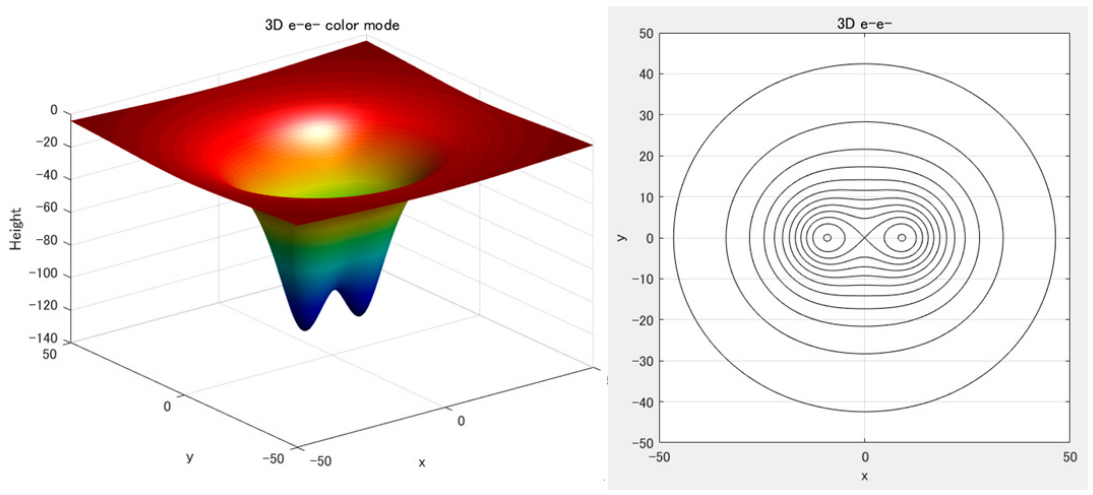
Figure A8 are standard three-dimensional diagrams of the electric fields generated by the two charges (-q, -q) in the three dimensional space. On the other hand, Figure 4 shows the electric fields generated by the two charges of -q separated by a distance of d=20 in a two-dimensional plane. Here, the parameters have been adjusted so that while the electric field in three-dimensional space follows F~1/r2, in two dimensions it follows F~1/r.
4.2. An Application of the Electric Dipole Field Model to the Gluon Field
Now, we need to explain why Figure 4 is applicable to the gluon field emitted by a quark. The electric field generated by a charge q in classical electromagnetism can be interpreted from the perspective of elementary particles as follows.
A charge q is associated with an energy fluctuation of ΔE over a short time interval Δt. The well-known uncertainty relation (ΔE·Δt ≈ ℏ) holds between the two. If, during the time interval Δt, there is no charge on the other side to receive this photon, the virtual photon returns to the original charge q. As a result of the repetition of this process, the electric field F ~ q2/r2 in classical electromagnetism ma be formed. It is believed that the same process also operates in the “strong force” between quarks mediated by gluons. Figure 4 was created by taking into account the electric field in a two-dimensional world, F~q2/r. In other words, could Figure 4 be regarded as the distribution of gluon density emitted by quarks? This is the reason why a two-dimensional dipole electric field was depicted here.
Since the coupling constant of the strong interaction is thought to be at least one order of magnitude larger than that of the electromagnetic force, the vacuum polarization effect of gluons related to the electromagnetic force shown in Figure 5 might not be negligible, and the effect of vacuum polarization may fill in the dip in the central part of Figure 4, causing the overall distribution to approach a rod-shaped distribution.
4.3. Semi-Classical Approach Under the Logarithmic Potential
Let us consider why the relationship shown in Figure 3 holds. To understand this intuitively, we will proceed with our discussion using a semi-classical quantum theory. Suppose the force acting between a quark and an anti-quark is described by F(r) = /r. Then, the potential energy can be written as V(r) = ·log(r/ro). Here ro (= ℏ/μv) is the de Broglie wavelength. Since we are considering meson systems, the reduced mass μ is half the mass of the quarks constituting the resonance states. Furthermore, the coupling constant is a function of the strong interaction coupling constant αs.
If the two-dimensional angular momentum ℓ is quantized according to semi-classical theory, the relationship ℓ = μv·r = nℏ holds. Since the two-dimensional centrifugal force μv2/r and the centripetal force /r balance each other, we obtain equation (8).
μv2/r = /r and = μv2
ℓ = μvr = nℏ, r = n·(ℏ/μv)
Equation (8) suggests that motion under the logarithmic potential involves constant kinetic energy. This is precisely the Virial theorem. It is known that the Virial theorem also holds in quantum mechanical world [11].
Figure 3 shows the results obtained when the principal quantum number n is increased by one at a time under m = 1. Equation (9) suggests that it holds not only for the angular momentum but also for variations in the principal quantum number. If we define the orbital radius r for the case n = 1 as ro, then the n-th r corresponds to a position that is an integer multiple of the de Broglie wavelength ro, <r(n)> =n ro. In other words, this suggests that the peak value of the radial density is a multiple of ro. Figure 3 is thought to reflect this fact. Furthermore, the energy level En of the n-th excited state of a quark and an antiquark can be written as follows, given that E = T + V and V(r) = –Vo + ·log(r/ro):
En = 1/2·μv2 – V0 + ·log(n) = 1/2· – V0 + ·log(n)
We believe this is the reason why the excited levels of charmonium and bottomonium can be represented by nearly straight lines on a semi-logarithmic graph. However, this equation cannot explain why the value of the slope holds not only for charmonium and bottomonium but also for the resonance levels of ρ-a2-ρ3-a4, which are composed of light quarks.
One hypothesis is that this may stem from the property that the strong interaction is a short-range force. That is, the strong interaction is determined by the well-known distance of 1.3 × 10⁻¹³ cm, inverse of pion mass, at that distance pions are virtually emitted and absorbed. It may be reasonable to assume that quark resonance occurs when a system consisting of a quark and an antiquark forms at a de Broglie wavelength that matches exactly within this strong interaction radius and its area of σ~40mb.
5. Summary
This paper examines why experimental data show that the excited states of charmonium and bottomonium—composed of heavy charm and bottom quarks, respectively—can be represented by nearly straight lines on a semi-logarithmic graph, even as an extremely good approximation. Incidentally, the correlation coefficient R for the four excited states of bottomonium (Υ(1S), Υ(2S), Υ(3S), and Υ(4S)) on a semi-logarithmic graph was 0.99997. There is an example that may provide a clue to the origin of the straight lines on the semi-logarithmic plot.
The potential energy V(r) in a 1/r force field is described by V(r) = ·log(r). Furthermore, in a 1/r force field, the virial theorem 2<T> = <r · dV/dr> suggests that the kinetic energy <T> remains constant. Consequently, since E = T + V(r), the eigenstate E is expected to reflect the form of V(r). Here, the logarithmic potential model is introduced as the force between q and . In contrast to the Cornell-type potential [15], V(r) = -4/3∙αs/r + kr2, which consists of a combination of two physical quantities—the Coulomb force and the spring force. The logarithmic potential automatically incorporates the concept of quark confinement and is characterized by weak divergence near the origin.
Numerical solutions to the Schrödinger equation for the three-dimensional logarithmic potential have been provided in previous studies [16,17]. However, since there are no examples of solving the two-dimensional Schrödinger equation to describe motion under the logarithmic potential, the authors solved it using the Numerov method to determine the eigenvalues. The primary conditions under which the solution was obtained were aligned with experimental data: total angular momentum (m) was fixed at m = 1, and the nodal quantum number (nr) was increased by one at a time. It was demonstrated that the six obtained eigenvalues could be represented by a straight line on a semi-logarithmic graph with a correlation coefficient of 0.998 (A8) Furthermore, it was found that the peak value of the radial density r|uu*| could also be represented by a straight line expected from semi-classical theory with a correlation coefficient R ~ 0.9996 (Figure 3). Based on the above results, it is believed that the quark-antiquark resonance states are realized in a state close to the two-dimensional x-y plane.
In this paper, we pointed out that, based on observed experimental data, it could be considered that the interaction between quarks and antiquarks occur in a two-dimensional space via gluons.
However we have not yet proven that it occurs in a two-dimensional space. In reality, the interaction may occur in three dimensional space, i.e., the gluon interactions occurs in a manner that is close to the two-dimensional space.
We predict that a solution to resolve this problem will be obtained if the spin-0 particle ηc(3S), formed by charm quarks, is experimentally confirmed. In the three dimensional space, extending the logarithmic plot predicts that ηc(3S) state lies at 4019.8 MeV. While an excited state does indeed exist at 4024.1MeV, however its isospin is 1 not 0, as would be expected from ηc(3S) state. On the other hand in the two dimensional case, the solution of the Schrödinger equation predicts at 3955MeV [7]. An enhancement has been already observed there as well, but the details still remains uncertain due to the small number of events around 3950 MeV. See Figure 3 of the paper on the experimental data [18].
Funding
This work was performed using the facilities of the Institute for Space-Erath Environment Research (ISEE), Nagoya University.
Data Availability Statement
All data we used are based on the data published by the Particle Data Group. We than the PDG group.
Acknowledgments
The authors acknowledge Prof. Yoshiki Teramto of Osaka Public University for very valuable comments given to the draft of the manuscript. The author thanks Prof. Shoichi Shibata of Chubu University for his many helpful comments during the editing this paper.
Conflicts of Interest
The authors declare no conflicts of interests.
Appendix A
Figure A6.
The normalized probability density |uu*| (in χ-space) is shown for various principle quantum number n=1 to 6. The vertical number presents the probability to find out the object within dr=0.01. The wave function has been obtained solving the two dimensional Schrödinger equation under the angular momentum m=1 and the potential of V(r) = −Vo + 8*log10(r).
Figure A6.
The normalized probability density |uu*| (in χ-space) is shown for various principle quantum number n=1 to 6. The vertical number presents the probability to find out the object within dr=0.01. The wave function has been obtained solving the two dimensional Schrödinger equation under the angular momentum m=1 and the potential of V(r) = −Vo + 8*log10(r).
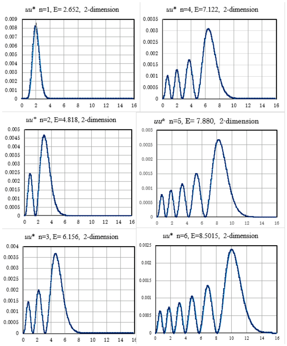
Figure A7.
The eigenvalues of the Schrödinger equation for the two dimensional case and three dimensional case are shown. The eigenvalues are plotted on the semi-logarithmic plane. The correlation coefficient of R for each process is also given. The eigenvalues are obtained under the conditions (a) the total angular momentum m=1 to 6 but the nodal quantum number is fixed to nr = 0. (the left side figure, for the two dimensional case) and (b) the nodal quantum number is fixed to nr=0 but the angular momentum ℓ increases from ℓ= 1 to 10 (the right side figure), for three dimensional case. The data points are referred from the paper of [16]). When we plot those eigenvalues from log10(2) (the red points), the correlation coefficient R increases.
Figure A7.
The eigenvalues of the Schrödinger equation for the two dimensional case and three dimensional case are shown. The eigenvalues are plotted on the semi-logarithmic plane. The correlation coefficient of R for each process is also given. The eigenvalues are obtained under the conditions (a) the total angular momentum m=1 to 6 but the nodal quantum number is fixed to nr = 0. (the left side figure, for the two dimensional case) and (b) the nodal quantum number is fixed to nr=0 but the angular momentum ℓ increases from ℓ= 1 to 10 (the right side figure), for three dimensional case. The data points are referred from the paper of [16]). When we plot those eigenvalues from log10(2) (the red points), the correlation coefficient R increases.
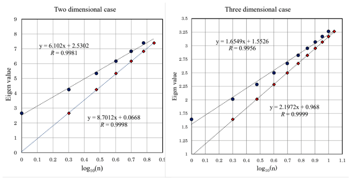
Figure A8.
The virtual photon density distribution in the three dimensional space produced by the dipole charge (e-, e-) separated with d=20 and the maximum height is 100 at the peaks. The contour is drawn every 10 difference of the field strength following F(r) ~ 1/r2.
Figure A8.
The virtual photon density distribution in the three dimensional space produced by the dipole charge (e-, e-) separated with d=20 and the maximum height is 100 at the peaks. The contour is drawn every 10 difference of the field strength following F(r) ~ 1/r2.
References
- Muraki, Y. A new mass formula of elementary particles. Progr. Theor. Phys. 1969, 41, 473–478. [Google Scholar] [CrossRef]
- Jackson, J. D.; Quigg, C.; Rosner, L. L. New Particles, Theoretical, Proceeding of the 19th International Conference on High Energy Physics (Tokyo) 1978 B8. (ICHEP78) CERN Document Server p391, New Particles, Theoretical by D, Jakson. Available online: https://cds.cern.ch/record/870666/files/c78-08-23-p391.pdf.
- Herb, S. W.; et al. Observation of a Dimuon Resonance at 9.5 GeV in 400-GeV Proton-Nucleus Collision. Phys. Rev. Lett. 1977, 39, 252–255. [Google Scholar] [CrossRef]
- Quigg, C.; Rosner, J. L. Quarkonium Level Spacings. Phys. Lett. 1977, B71, 153–157. [Google Scholar] [CrossRef]
- The Belle II Collaboration, Adachi et al., Study of Υ(10753) decays to π+π-Υ(nS) final states at Belle II. J. High Energy Phys. 2024, 7, 116. [CrossRef]
- Atabek, O.; Deutsch, C.; Levaud, M. Schrodinger equation for the two-dimensional Coulomb potential. Phys. Rev. 1974, A9, 2617–2624. [Google Scholar] [CrossRef]
- Muraki, Y.; Shibata, S. A Meson Binding-state Model in the Two-Dimensional Space. Particles 2026, 9, 55–67. [Google Scholar] [CrossRef]
- Muraki, Y.; Shibata, S. Prediction of Toponium mass using Logarithmic Potential model. Proceed. 39th ICRC in Geneva, 2025; PoS(ICRC2025) 341. [Google Scholar] [CrossRef]
- Simons, T. E. A Numerov-type method for the numerical solution of the radial Schrödinger equation. Appl. Numer. Methods 1991, 7, 201–206. [Google Scholar] [CrossRef]
- Vigo-Aguiar, J.; Ramos, H. A variable-step Numerov method for the numerical solution of The Schrödinger equation. J. Math. Chem. DOI. 2005, 37, 255–262. [Google Scholar] [CrossRef]
- Bransden, B. H.; Joachain, C. J. Physics of Atoms and Molecules, published in 1983; Longman Scientific and Technical; pp. page 147–148.
- Gross, F. Klempt, E. Brodsky, SJ. et al. 50 years of Quantum Chromodynamics. Eur. Phys. J. (figure 4.3.6). 2023, C83 72, 1125. [CrossRef]
- Bissey, F. Gluon flux-tube distribution and linear confinement in baryons. Phys. Rev. 2007 D76, 114512. [Google Scholar] [CrossRef]
- Bissey, F. Gluon flux-tube distribution and linear confinement in baryons. Phys. Rev. 2007, D76, 114512. [Google Scholar] [CrossRef]
- Bali, G.s.; Schuilling, K.; Schlichter, C. Observation of long color flux tube in SU(2) lattice gauge theory. Phys. Rev. 1995, D51, 5165–5198. [Google Scholar] [CrossRef]
- Eichten, E. Gottfried, K. Kinoshita, T. Lane, K.D. and Yan, T-M., Charmonium: The model. Phys. Rev. 1978, 3090–3117. [CrossRef]
- Ciftci, H.; Ateser, E.; Koru, H. The power-law and the logarithmic potentials. J. Phys. A Math. Gen. 2003, 36, 3821–3828. [Google Scholar] [CrossRef]
- Roy, A. K. Calculation of the bound states of power-law and logarithmic potentials through a generalized pseudo spectral method. J. Phys. G. Nucl. Part. Phys. 2004, 30, 269–278. [Google Scholar]
- The Belle collaboration, Observation of a Charmonium-like State Produced in Association with a J/ ψ Annihilation at √s =10.6 GeV. Phys. Rev. Lett. 2007, 98 082001. [CrossRef]
Figure 1.
The experimental mass data of the bottomonium (left) and charmonium (right) are plot ted on the semi-logarithmic plot. The correlation coefficients R between the data points and the linear line are 0.997 and 0.995 respectively. On the bottomonium plot, we include three higher states of the bottomonium recently observed by the Belle II experiment with rather wide spread [5]. However, when we use the four experimental points with the sharp width, the correlation coefficient R turns out as 0.99997 (four nines!). Here, Υ1 to Y4 correspond to Υ(1S) to Υ(4S) states, respectively.
Figure 1.
The experimental mass data of the bottomonium (left) and charmonium (right) are plot ted on the semi-logarithmic plot. The correlation coefficients R between the data points and the linear line are 0.997 and 0.995 respectively. On the bottomonium plot, we include three higher states of the bottomonium recently observed by the Belle II experiment with rather wide spread [5]. However, when we use the four experimental points with the sharp width, the correlation coefficient R turns out as 0.99997 (four nines!). Here, Υ1 to Y4 correspond to Υ(1S) to Υ(4S) states, respectively.
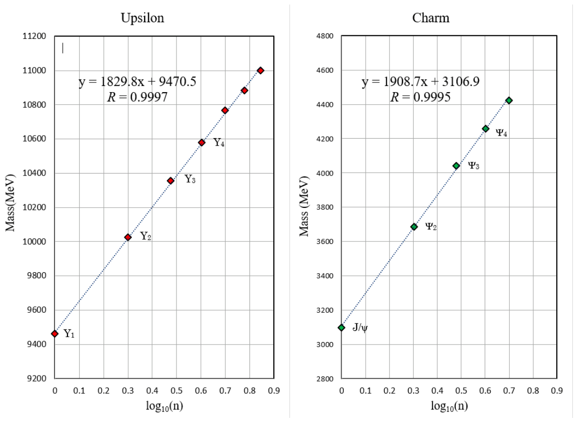
Figure 2.
The radial density distribution r|uu*| in χ-space or radial distribution function in f-space of the two dimensional Schrödinger equation for the principal quantum number (n) changing form n=1 to 6 under the total angular momentum m=1. The vertical axis represents the normalized probability amplitude within dr=0.01 multiplied the distance r from the origin, while the horizontal axis presents the distance from the origin. The wave function (u) has been derived numerically under the potential of V(r) = − Vo + 8*log10(r).
Figure 2.
The radial density distribution r|uu*| in χ-space or radial distribution function in f-space of the two dimensional Schrödinger equation for the principal quantum number (n) changing form n=1 to 6 under the total angular momentum m=1. The vertical axis represents the normalized probability amplitude within dr=0.01 multiplied the distance r from the origin, while the horizontal axis presents the distance from the origin. The wave function (u) has been derived numerically under the potential of V(r) = − Vo + 8*log10(r).
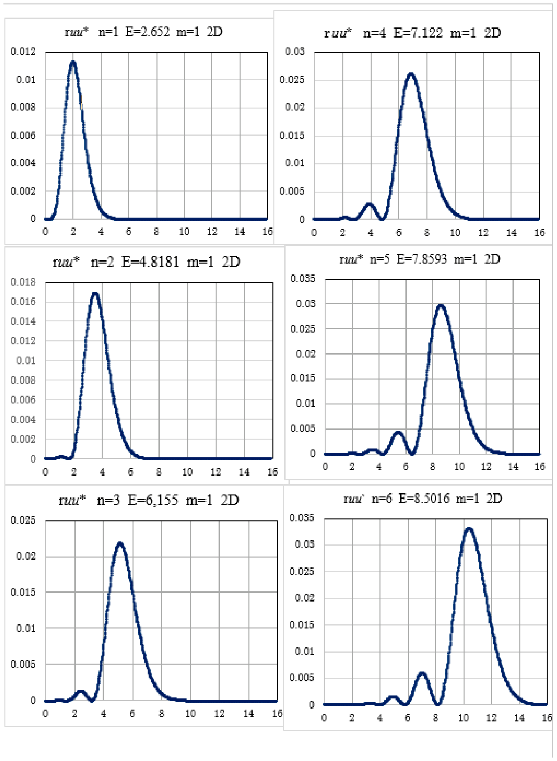
Figure 3.
The most probable radius predicted by the two dimensional Schrödinger equation is plotted for the principal quantum number (n) from n=1 to 6. The peak radius of the density distribution may be fit by the linear line under the correlation coefficient R= 0.9996.
Figure 3.
The most probable radius predicted by the two dimensional Schrödinger equation is plotted for the principal quantum number (n) from n=1 to 6. The peak radius of the density distribution may be fit by the linear line under the correlation coefficient R= 0.9996.
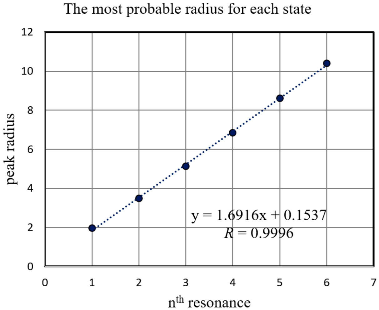
Figure 4.
The photon density distribution, induced by the electric di-pole, on the two dimensional plane (on the x-y plane) is shown to the case of the dipole distance of d=20. The density distribution is shown by the contour lines. The lines are drawn by every 10 difference of height of which the peak value is assumed as 100. The electric filed distribution is assumed to follow E(r) ~1/r. It would be interesting to compare this picture with the gluon distribution obtained by the lattice QCD calculation [12,13,14].
Figure 4.
The photon density distribution, induced by the electric di-pole, on the two dimensional plane (on the x-y plane) is shown to the case of the dipole distance of d=20. The density distribution is shown by the contour lines. The lines are drawn by every 10 difference of height of which the peak value is assumed as 100. The electric filed distribution is assumed to follow E(r) ~1/r. It would be interesting to compare this picture with the gluon distribution obtained by the lattice QCD calculation [12,13,14].
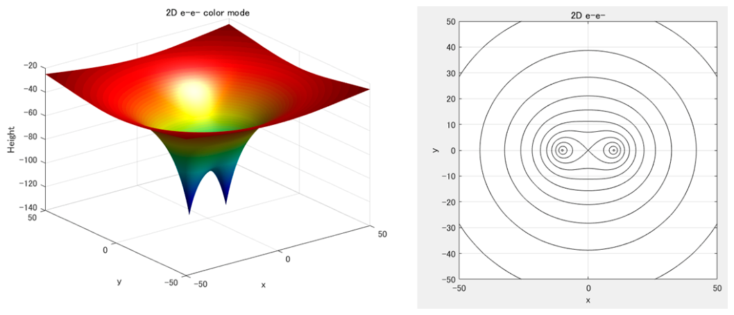
Figure 5.
(a) The Feynman diagram for the vacuum polarization process and (b) gluon pair production process in the gluon exchange process. In the case of the electromagnetic interaction, the diagram (a) happens 10-4 times less than the single photon exchange process, however in the strong interaction process, the process of (b) may happen. However, in present simple discussions, we did not taken account of this effect.
Figure 5.
(a) The Feynman diagram for the vacuum polarization process and (b) gluon pair production process in the gluon exchange process. In the case of the electromagnetic interaction, the diagram (a) happens 10-4 times less than the single photon exchange process, however in the strong interaction process, the process of (b) may happen. However, in present simple discussions, we did not taken account of this effect.
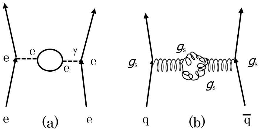

Table 1.
captions: From left to right; these correspond to the types of quarks constituting the reso nance state, the correlation coefficient R when plotted starting from principal quantum number n=1, the correlation coefficient R when plotted starting from n+1, the number of excited states used for plotting, the estimated masses of the constituent quarks, and the slope and intercept of the line when plotted on a semi-logarithmic graph (units: MeV/c2).
Table 1.
captions: From left to right; these correspond to the types of quarks constituting the reso nance state, the correlation coefficient R when plotted starting from principal quantum number n=1, the correlation coefficient R when plotted starting from n+1, the number of excited states used for plotting, the estimated masses of the constituent quarks, and the slope and intercept of the line when plotted on a semi-logarithmic graph (units: MeV/c2).
| Series (kind of Quarks) |
R from n |
R from n+1 |
Number of points |
quark mass | Slope and intercept Mass(MeV/c2)= |
|---|---|---|---|---|---|
| Bottomonium (ϒ) (b) | 0.99997 | 0.9952 | 7 | 4.18 GeV | 1829.8∙log(n)+9470.5 |
| Charmonium (J/ψ) (c) | 0.9991 | 0.9952 | 5 | 1.27 GeV | 1908.7∙log(n)+3106.9 |
| ρ-a2-ρ3-a4 (u, d) | 0.9987 | 0.9999 | 4 | 2.2, 4.7 MeV | 1975∙ log(n) +757 |
| N*(1/2) (u, d) | 0.9990 | 0.9955 | 6 | 2.2, 4.7 MeV | 1614∙ log(n) +941.4 |
| Ω- (3/2) ( s ) | 0.9992 | 0.9951 | 5 | 93 MeV | 1189∙ log(n) +1668 |
Disclaimer/Publisher’s Note: The statements, opinions and data contained in all publications are solely those of the individual author(s) and contributor(s) and not of MDPI and/or the editor(s). MDPI and/or the editor(s) disclaim responsibility for any injury to people or property resulting from any ideas, methods, instructions or products referred to in the content. |
© 2026 by the authors. Licensee MDPI, Basel, Switzerland. This article is an open access article distributed under the terms and conditions of the Creative Commons Attribution (CC BY) license (http://creativecommons.org/licenses/by/4.0/).
Copyright: This open access article is published under a Creative Commons CC BY 4.0 license, which permit the free download, distribution, and reuse, provided that the author and preprint are cited in any reuse.