
Submitted:
26 August 2026
Posted:
27 August 2026
You are already at the latest version
Abstract
Artificial spin ice systems have provided powerful platforms for exploring frustrated magnetism and emergent phenomena. However, nanoscale fabrication constraints limit the direct manipulation and real-time visualization of individual magnetic elements for square ice model. Macroscopic mechanical analogues overcome these limitations by enabling direct observation and flexible control of local interactions. Nevertheless, how geometry-tuned intra-unit interactions regulate global ordering in frustrated systems remains poorly understood. Here, we construct a “macroscopic square ice” experimental platform to investigate this problem, using the unit gap l as a tunable geometric parameter while fixing the vertex gap d at 1.1 mm. By directly monitoring magnetic domain evolution and vertex-type distributions, we reveal a non-monotonic order–disorder–order transition driven by the competition between intra-unit and inter-vertex interactions. This work provides direct experimental insight into the role of geometry-controlled local interactions in governing collective ordering and offers a visible approach for studying emergent behaviors in frustrated systems.
Keywords:
square ice model
; macroscopic square ice
; non-monotonic geometric dependence
; frustration
; unit gap
1. Introduction
Geometric frustration refers to constraints that prevent simultaneous minimization of all interactions, leading to a highly degenerate ground state and the emergence of novel phenomena. The square ice model is a representative classical frustrated system and reveals the mathematical essence of frustration in spin ice—the impossibility of graph-coloring in certain cases. In the square-ice model, at each vertex the four nearest-neighbor spins satisfy the “two-in, two-out” ice rule; the ground-state manifold is highly degenerate, providing a suitable theoretical framework to study emergent excitations and phase behavior in frustrated systems. Artificial spin ice systems based on nanoscale magnetic islands have experimentally realized the square ice model’s ground-state manifold and enabled observation of magnetic monopole excitations, Dirac strings, and Coulomb phases. However, due to ultrafast spin dynamics and limitations of nanoscale characterization, direct tracking of spin flips and vertex rearrangements remains challenging, leaving gaps in understanding the mechanisms and evolution of square ice. Macroscopic frustrated systems with limited degrees of freedom have traditionally struggled to reproduce the complete ground-state manifold and its evolution. In response, we designed a macroscopic square ice platform comprising hundreds to thousands of NdFeB magnets confined in vertical cylindrical wells on a PMMA base, each unit containing two magnets of different heights. The platform offers three advantages: (1) room-temperature optical observation enables direct recording; (2) unit gap l and vertex gap d can be independently tuned to study intra-unit vs vertex interactions; (3) vertex types and magnetic-domain evolution can be tracked throughout, providing a visual method to study evolution in frustrated systems. This study focuses on how intra-unit interactions regulate the non-monotonic evolution in the square ice model. By fixing d = 1.1 mm and varying l from 9.7 mm down to 0.7 mm, we observe the evolution of vertex-type proportions and magnetic-domain sizes. We find that as l decreases (increasing intra-unit interaction), the system experiences a non-monotonic evolution. At l ≈ 9d, the system is excited ordered due to abundant excited units and mostly ice-rule vertices; at l ≈ 1.4d and 2.1d, long-range antiferromagnetic order emerges; at l ≈ d, the Type-I vertex fraction plunges and disordered states appear; for l = 0.64d, the system re-enters an antiferromagnetic order. Magnetic structure factor analysis shows qualitative characteristic features that motivate a possible connection to constrained-string physics. This work provides the direct optical imaging of assembled configurations for frustrated system ordering at the macroscopic scale and offers a tunable platform for exploring topological excitations and evolution.
2. Experimental Methods
2.1. Sample Design and Geometry
Macroscopic square ice consists of hundreds to thousands of NdFeB magnets arranged in a square lattice on a PMMA base. Each magnet is confined in a cylindrical well slightly larger than the magnet diameter, permitting only two vertical states: up or down. The well depth is 10 mm to ensure adequate vertical space. Each unit contains two magnets with different heights (long: 6 mm, short: 5 mm), representing a pseudo-spin. There are two possible ground states: (a) left magnet up, right magnet down (pseudo-spin left) and (b) left long magnet down, right short magnet up (pseudo-spin right). All magnets are oriented with the North pole up; the long and short magnets are staggered in the lattice. The minimum horizontal spacing within a unit defines the unit gap l (Figure 1(b)); l values used are 9.7, 2.3, 1.5, 1.1, and 0.7 mm to tune intra-unit magnetic interactions.
The four neighboring units meet at a vertex; the minimum distance between the two adjacent units defines the vertex gap d, fixed at 1.1 mm, enabling analysis of intra-unit vs vertex interactions. The pseudospin direction is determined based on the absolute height of the magnets and the relative vertical displacement between the centers of two adjacent magnets. The difference between the center heights of the first and second magnets is denoted as Z. Taking the trap bottom as zero, the height of the magnet top relative to the trap bottom is called the absolute height. When a magnet exhibits the up state, the threshold (minimum) of the absolute height is 9.5 mm; when it exhibits the down state, the threshold (maximum) is 6.5 mm. In principle, a magnet could have an intermediate state, with its absolute height between 4.5 mm and 5.5 mm. Two up magnets form an up-up unit, with Z ranging from -0.5 mm to 0.5 mm. Its pseudospin is represented by two outward arrows. Two down magnets form a down-down unit, with Z ranging from -0.5 mm to 0.5 mm, and its pseudospin is represented by two inward arrows. The spin magnitude is 1. Magnets in intermediate states are extremely rare in the square lattice; in such cases, and the intermediate-state magnet is represented by a fractionalized spin, marked as two small arrows, with spin magnitude 1/2. At this point, all possible states of a unit have been assigned pseudospins. According to the real parameters, positions and magnetic flux density, unit energy (interaction energy of two magnets in a unit) can be obtained by Comsol for different Z (Figure 1(d)).
2.2. Vertex Types and Classification Criteria
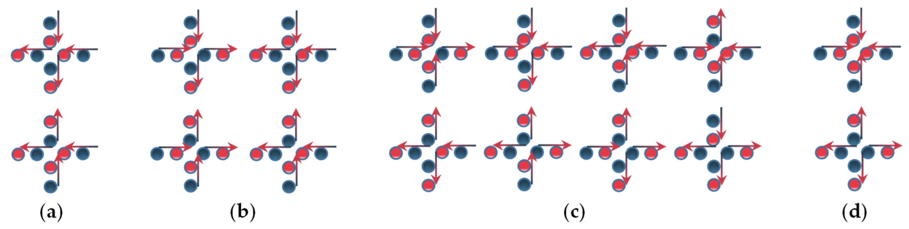
At a vertex, four pseudo-spins (one per unit) only with unit ground states create 16 configurations. Following square ice and artificial spin ice conventions, these configurations are grouped into four classes: Type I (2-in-2-out ice rule; 2 configurations; lowest energy), Type II (2-in-2-out ice rule; 4 configurations; next-lowest energy), Type III (3-in-1-out or 1-in-3-out; 8 configurations; monopole excitations; higher energy), Type IV (4-in or 4-out; 2 configurations; highest energy; rare). I and II comply with ice rule; III and IV violate it. The four vertex types are illustrated with dark magnets down and red magnets up; arrows denote pseudo-spin directions. In a fully random array, the proportions are 12.5%, 25%, 50%, and 12.5% for Type I–IV, respectively.
Figure 2.
Vertex types in macroscopic square ice. (a) Schematic of Type-I vertices. Vertex gap d is fixed to be 1.1 mm. (b) Schematic of Type-II vertices, where pseudospins share the same direction for each row and each column. (c) Schematic of Type-III vertices, which are elementary excitations in macroscopic square ice. (d) Schematic of Type-IV vertices, which rarely appear in the system.
Figure 2.
Vertex types in macroscopic square ice. (a) Schematic of Type-I vertices. Vertex gap d is fixed to be 1.1 mm. (b) Schematic of Type-II vertices, where pseudospins share the same direction for each row and each column. (c) Schematic of Type-III vertices, which are elementary excitations in macroscopic square ice. (d) Schematic of Type-IV vertices, which rarely appear in the system.
When vertex types include up-up and down-down units, the number of vertex configurations can be expanded to 256, among which there are 32 configurations for Type-I vertices, 64 for Type-II vertices, 128 for Type-III vertices, and 32 for Type-IV vertices. The vertex configuration is mainly determined by the states of the inner four magnets of the vertex, while the outer four magnets of the vertex can be in arbitrary states, thus multiplying the original number of configurations by 16 and generating a large number of new configurations. The correlation U between the two magnets in up-up and down-down units is 1, which does not affect the nearest-neighbor correlation I of the vertex; the nearest-neighbor correlations of Type-I and Type-IV vertices remain -1 and 1, respectively, and those of Type-II and Type-III vertices remain 0. The correlation function L is also unaffected; the L correlations of Type-I, Type-II, Type-III, and Type-IV vertices remain 1, -1, 0, and 1, respectively. Besides affecting the unit correlation function U, up-up and down-down units also change the next-nearest-neighbor correlation L. At this point, the next-nearest-neighbor correlation L cannot be calculated by simple rules and must be analyzed vertex by vertex. In the calculation of the magnetic structure factor, to describe up-up and down-down units and distinguish them from ordinary up-down units, this study uses 11 to represent an up-up unit, 00 to represent a down-down unit, and 01 and 10 to represent different up-down units. The magnet states in each row of horizontal units are represented by binary symbols, with 1 denoting a magnet up and 0 denoting a magnet down. The states of each row of horizontal units are converted into row vectors, and the overall state of the horizontal units is transformed into a matrix. The magnet states in each column of vertical units are also represented by the same binary symbols; then the states of each column of vertical units form a row vector, and the states of all vertical units are transformed into another matrix. These two matrices are then fed into a computer program, which can automatically generate the magnetic structure factor. The magnetic structure factor is computed according to the real positions of magnets.
2.3. Sample Preparation and Assembly
To control variables, all samples use a consistent assembly. In the PMMA base, horizontal unit rows are filled with magnets in a sequence as shown in Figure 3(a); neighboring units have opposite magnet order, and adjacent rows have opposite horizontal order. Vertical units follow a similar scheme. This assembly tends to promote Type-I vertices and enhances near-neighbor interactions, while stronger intra-unit interactions may induce Type-II and Type-III vertices spontaneously. Vertex energy is shown in Figure 3(c).
To quantitatively characterize the degree to which the system satisfies the ice rule, this work defines two derived physical quantities: (1) the ice-rule satisfaction rate Rice = (NI + NII)/Ntotal, which equals the sum of the proportions of Type-I and Type-II vertices, reflecting the overall proportion of vertices satisfying the ice rule; (2) the monopole excitation density ρmono = (NIII + 2NIV)/Ntotal, reflecting the proportion of vertices that break the ice rule, where NI, NII, NIII, and NIV denote the numbers of the corresponding vertex types, and Ntotal is the total number of vertices. Since Type-IV vertices are rare, the monopole excitation density is approximately equal to the proportion of Type-III vertices.
2.4. Experimental Parameter Characterization
To support the consistency of sample preparation, this study systematically measured and statistically analyzed the key geometric and magnetic parameters of the traps and magnets used in the experiments. As shown in Figure 4(a), the key geometric parameter of the trap is the trap diameter D′. The distribution of the trap diameter D′ is shown in Figure 4(b). One hundred traps were randomly selected for measurement; their diameters range from 3.88 to 4.88 mm, with a mean value of 4.37 mm and a standard deviation of 0.15 mm, approximately following a Gaussian distribution. Optical images and schematic diagrams of the two types of magnets are shown in Figure 4(c). Both types of magnets have the same diameter D, whose distribution is shown in Figure 4(d), with a mean value of 3.97 mm and a standard deviation of 0.03 mm. Their heights are denoted as h1 and h2. The magnetic flux densities and masses are denoted as B1, B2, m1, and m2, respectively.
One hundred short magnets and one hundred long magnets were selected, and their magnetic flux densities, masses, and heights were measured individually. The measurement results are shown in Figure 5, Figure 6 and in Table 1 and Table 2. The mean values and standard deviations of each parameter are given in the second and third rows of Table 1 and Table 2, respectively. Gaussian fitting (red curves) shows that all parameters approximately follow Gaussian distributions, indicating good consistency of the magnets. The mean values of the magnetic flux density B1, mass m1, and height h1 of the short magnets are 253.7 mT, 0.47 g, and 4.96 mm, respectively; the corresponding values for the long magnets are 278.2 mT, 0.55 g, and 5.77 mm. The actual heights of the two types of magnets are in good agreement with the design values (5 mm and 6 mm).
For ease of description, this study classifies the system states into three categories based on the characteristic features of the magnetic structure factor: states in which bow-tie diffuse characteristic features occur are called excited ordered states (EO); states in which the magnetic structure factor shows only antiferromagnetic Bragg peaks are called antiferromagnetic ordered states (AFM); states in which antiferromagnetic and ferromagnetic Bragg peaks coexist are called disordered states (DS). It should be noted that the term "state" here is used only to describe the experimentally observed orderliness, and does not correspond to a strict thermodynamic phase.
3. Results
As l decreases, intra-unit interactions become stronger. Figure 7 shows the spatial distribution of vertex types as a function of l. At l = 9.7 mm, nearly all vertices are Type-I, forming a large connected Type-I domain. Because most units are in excited configurations, the system is identified as an excited ordered state. When l is reduced to 2.3 mm and 1.5 mm, Type-I domains remain dominant, but Type-II and Type-III domains emerge in some regions, yielding an antiferromagnetic-like ordered state. At l = 1.1 mm, the Type-I vertex fraction drops to 36.36%, while Type-II and Type-III rise significantly, placing the system in a disordered state with a high monopole density. With a further reduction of l to 0.7 mm, Type-I domains re-grow and Type-II / Type-III domains shrink, partially restoring antiferromagnetic order. This “order–disorder–order” evolution is referred to as non-monotonic behavior.
It is found that the ratio between the unit gap l and the vertex gap d determines the evolution of system order. When l gradually decreases from far greater than d to less than d, the system shows a non-monotonic geometric dependence: when l ≈ 9d, Type-I vertices dominate, although a large fraction of units remain in excited states, resulting in an excited ordered state; l ≈ 1.4d and 2.1d, Type-I vertices dominate and most units are in their ground states, exhibiting long-range antiferromagnetic order; when l ≈ d, the proportion of Type-I vertices drops sharply to 36.36%, while the proportions of Type-II and Type-III (monopole excitation) vertices rise significantly, and the system enters a highly disordered state; when l = 0.64d, the proportion of Type-I vertices rebounds to 78.79%, and antiferromagnetic order is restored. The above evolution originates from interaction competition.
3.1. Vertex Proportions and Evolution of Order
Figure 8(a) shows the states for five sample sets: Type-I, Type-II, and Type-III vertex proportions vs l. When l decreases from 9.7 mm to 0.7 mm, a pronounced non-monotonic evolution is observed. At l ≈ 9d, Type-I vertices dominate with almost all vertices obeying ice rules, but many units are excited (inelastic to gravity), producing an excited ordered state. When l ≈ 1.5 mm (≈ 1.4d), Type-I remains dominant and most units are in ground states, yielding long-range antiferromagnetic order. At l ≈ d (1.1 mm), the Type-I vertex fraction decreases sharply to 36.36%, while II and III rise to 24.52% and 39.12%, respectively, indicating a disordered state with a high monopole density. When l decreases to 0.7 mm, the Type-I rises to 78.79% and antiferromagnetic order partly recovers. The evolution is attributed to interaction competition.
The states and correlation data (Figure 8) show that the nearest-neighbor correlation of Type-I vertices and next-nearest-neighbor correlation L vary with l in a manner that tracks vertex-type proportions, with a notable minimum near l = d, indicating maximal competition. Figure 8(a) shows the states of macroscopic square ice, presenting the variations of the proportions of Type-I, Type-II, and Type-III vertices with l for five groups of samples. When l decreases from 9.7 mm to 0.7 mm, the system shows a significant non-monotonic evolution. When l = 9.7 mm (about 9d), the proportion of Type-I vertices is 97.22%, while the proportions of Type-II and Type-III vertices are both close to zero. At this point, almost all vertices satisfy the ice rule; however, it is noteworthy that a large number of the two magnets within each unit are simultaneously in the up or down excited states.
This can be attributed to the intra-unit magnetic interaction and vertex interaction. For the first row of horizontal units, all magnets are down because the intra-unit magnetic interaction is too weak to overcome the gravitational weight of the magnets. The next row of vertical units will be in the ground state because the upper half of the magnets is stabilized by vertex interactions to be up while the lower half is governed by gravity, resulting in a downward alignment. For the remaining horizontal units, the vast majority of macroscopic magnets are supported by vertex interactions and thus align upward, with only a small number at the boundaries deviating from this state. For the remaining vertical units, the magnets are simultaneously influenced by gravity and the downward repulsive vertex interaction exerted by the horizontal-unit magnets; consequently, except for a few boundary magnets, all are aligned downward. The system is highly ordered with many up-up units and down-down units, so this state is called an “excited ordered state (EO)”.
As l decreases to 1.5 mm (about 1.4d), the proportion of Type-I vertices drops to 84.35%, while the proportions of Type-II and Type-III vertices rise slowly. At this point, the intra-unit interaction has become strong enough to stabilize most units in their ground states, and the system enters ground states at both the vertex and unit levels, thereby establishing long-range antiferromagnetic order. When l is further reduced to 1.1 mm (i.e., l = d), the vertex proportions change dramatically: The Type-I vertex fraction decreases sharply to 36.36%, while the proportions of Type-II and Type-III vertices jump to 24.52% and 39.12%, respectively. At this point, the proportions of both Type-I and Type-II vertices are below 50%, the ice-rule satisfaction rate (I + II) is only 55.62%, and the magnetic monopole density is as high as 39.12%, indicating that the system has entered a highly disordered state with a high monopole density. This state arises because the intra-unit interaction and the inter-vertex magnetic interaction become comparable in strength; the friction between the first magnet of a unit and the trap wall is large enough to overcome gravity and keep it in the up state, while the second magnet is down, causing the pseudospin of the unit to reverse. This process is called unit flipping. One unit flip can turn a Type-I vertex into a Type-III vertex, while two unit flips turn it into a Type-II vertex; therefore, the proportion of Type-III vertices is usually higher than that of Type-II vertices, which is consistent with the experimental results. When l decreases from 1.5 mm to 1.1 mm, macroscopic square ice evolves from an antiferromagnetic state to a disordered state; when l decreases from 1.1 mm to 0.7 mm, it returns from the disordered state to the antiferromagnetic state [71].
When l decreases to 0.7 mm (0.64d), the proportion of Type-I vertices rebounds to 78.79%. The proportion of Type-III vertices drops to 15.15%, and the ice-rule satisfaction rate recovers to 73.37%, with antiferromagnetic order partially restored. From an energy perspective, Type-I vertices have the lowest interaction energy, so when only one type of interaction is present, the system preferentially forms Type-I vertices. However, the system involves interaction competition. Therefore, as l decreases, the system undergoes the non-monotonic evolution. For l takes the values of 9.7, 2.3, 1.5, 1.1 and 0.7 mm, the numbers of samples are all three. Repeated experiment shows that the standard deviations of vertex proportions are all below 13%. With the number of vertices fixed to be 121, non-monotonic evolution occurs in representative samples. For the proportion of Type-I vertices, the largest standard deviation 12.83% occurs at l = 1.1 mm and the least standard deviation 3.91% occurs at l = 2.3 mm (Table 3). For the proportion of Type-II vertices, the largest standard deviation 9.29% also occurs at l = 1.1 mm, but the least standard deviation 0.95% occurs at l = 0.7 mm (Table 4). For the proportion of Type-III vertices, the largest standard deviation 9.02% occurs at l = 0.7 mm and the least 1.52% occurs at l = 9.7 mm (Table 5).
3.2. Supporting Evidence from Correlation Functions, Unit Proportions, and Domain Sizes
The changes in correlation functions further support the above evolution trend. Figure 8(b) shows the variation of the correlation strengths of nearest-neighbor I and next-nearest-neighbor L with l. The inset shows the positional relationship among nearest-neighbor I, next-nearest-neighbor L, and the gray magnet: all three are located at the same vertex; the two I magnets are respectively at the upper-left and lower-left positions of the gray magnet, and the L magnet is collinear with the unit containing the gray magnet. When l decreases from 2.3 mm to 1.1 mm and then to 0.7 mm, the nearest-neighbor I correlation changes from -0.98 to -0.47 and then recovers to -0.82; the next-nearest-neighbor L correlation changes from 0.92 to 0.26 and then rebounds to 0.77. The extrema of the correlation functions occur at l = d, in full agreement with the changes in vertex proportions. Overall, as l decreases, the correlation functions exhibit an evolution trend similar to that of the vertex proportions, reflecting changes in the system order, with weak correlations occurring exactly at l = d.
When the two magnets have equal lengths, the magnets with flush tops have horizontal interactions, which tend to form excited states. To minimize the occurrence of excited states, this work adopts magnets of different lengths. When the magnet tops are flush, the interactions along the vertical direction between magnets can reduce excited states. The up and down states of the magnets correspond to the north and south poles of ferromagnetic nanoislands, respectively. To avoid a significant difference in magnetic flux density at the two ends of a pseudospin, the length difference between the long and short magnets is only 1 mm. The interaction energy of a unit depends only on the relative vertical displacement between the centers of the two magnets; the vertical displacement, mass, and magnetic flux density between the long and short magnets do not break the energy degeneracy of the two pseudospin directions. Odd numbers represent short magnets, marked in blue, and even numbers represent long magnets, marked in red. In horizontal units of odd-numbered rows, the magnet order follows a 1243 cycle; in even-numbered rows, the corresponding two units show a 2134 cycle. For vertical units, from the first column to the last column, the magnet order of every two units in odd-numbered columns follows a 2134 cycle, while that in even-numbered columns follows a 1243 cycle. For horizontal units in adjacent rows, the magnet orders are opposite. For vertical units in adjacent columns, the magnet orders are also opposite. At the boundaries, the magnet orders of the first row of horizontal units and the first column of vertical units are given, while those of the last row of horizontal units and the last column of vertical units should be determined according to the parity of the row and column numbers.
As shown in Figure 8(c), when l is 9.7 mm, the proportion of up-down units is only 15.11%, while the proportions of up-up and down-down units are 39.97% and 44.92%, respectively. When l decreases to 2.3 mm, the proportion of up-down units reaches 93.91%, and the proportions of up-up and down-down units drop to 2.24% and 3.85%, respectively. As the intra-unit interaction strengthens, the proportions of up-up and down-down units decrease significantly.
The magnetic domain size is defined as the maximum number of vertices within a single domain. The changes in the sizes of Type-I, Type-II, and Type-III domains at l = 9.7 mm, 2.3 mm, 1.5 mm, 1.1 mm, and 0.7 mm are detailed in Table 6. The maximum size of Type-I domains gradually decreases from 118 vertices at l = 9.7 mm to 30 vertices at l = 1.1 mm, and then rebounds to 68 vertices at l = 0.7 mm. The size of Type-III domains increases monotonically from 0 to 17 vertices, and does not decrease significantly when l = 0.64d, indicating that monopole excitations are more likely to nucleate and aggregate under strong interaction conditions, but remain smaller than Type-I domains (Table 7).
An energy competition model can qualitatively explain this phenomenon. Vertex proportions are related not only to the interaction energy but also to the assembly method. Because magnets interact with each other during the process, which is similar to the mutual collisions of microscopic molecules, the effect of the assembly method can be attributed to an energy barrier. The energy barrier is related to the number of unit flips. Under a given assembly method, the fewer the unit flips required for a vertex, the lower its energy barrier. Type-II vertices require more unit flips than Type-III vertices, so the energy barrier of Type-II vertices is higher than that of Type-III vertices, and the proportion of Type-III vertices is generally higher than that of Type-II vertices. As shown in Table 8 and Table 9, Type-II domains are generally smaller than Type-III domains. Since Type-III vertices can be regarded as elementary excitations, macroscopic square ice provides new macroscopic experimental evidence for studying elementary excitations in frustrated systems.
3.3. Magnetic Structure Factor
In addition to vertex proportions, correlation functions, and domain sizes, the magnetic structure factor can also effectively characterize the magnetic order of the system. The image of the magnetic structure factor can reveal information about magnetic order, evolution, and quasiparticle excitations; therefore, its calculation is of great significance. For l equals 2.3 mm, 1.5 mm, 1.1 mm and 0.7 mm, the proportion of the ground state of units is over 80%. Most units can be regarded as an Ising spin according to real positions of magnets. Following the conventional calculation method for the magnetic structure factor in artificial spin ice, the magnetic structure factor I(q) of macroscopic square ice is defined as follows.
Definition 1.
Let Si be the pseudospin of the i-th unit, ri be the position of the i-th unit, q be the reciprocal lattice vector, and N be the total number of pseudospins. Then the magnetic structure factor I(q) is expressed as
In Eq. (1), Si denotes the spin of the i-th site. ri is the position of site i, and q is the scattering vector. ⟨···⟩ denotes the thermal average. When q = 0, I (0) can be expressed as
The calculation method of the magnetic structure factor is given by Eqs. (1) and (2), and the results are shown in Figure 9, reflecting the evolution of system order from the reciprocal-space perspective.
I (0) = (1/N)∑i,j⟨Si·Sj⟩ = (1/N) ⟨(∑iSi)2⟩
When l = 9.7 mm, the magnetic structure factor cannot be calculated by Eqs. (1) and (2). This suggests that the evolution from this excited ordered state to the antiferromagnetic state may be related to string-like excitations. When l decreases to 2.3 mm or even 1.5 mm (Figure 9(a)), the magnetic structure factor shows sharp antiferromagnetic Bragg peaks at the Brillouin zone boundaries such as (π, π), consistent with the real-space antiferromagnetic order.
When l = 1.1 mm (Figure 9(b)), the intensity of the antiferromagnetic Bragg peaks is significantly weakened, and ferromagnetic Bragg peaks also appear at the zone center. The two types of Bragg peaks coexist, both with relatively low intensity, indicating that the system exhibits a disordered state. Notably, this state shows two types of Bragg peaks, which is distinctly different from the excited ordered state at l = 9.7 mm in terms of reciprocal-space characteristics. This indicates that the disordered state at l = 1.1 mm shows coexistence of multiple ordered components.
For l = 0.64d, Type-I vertex fraction recovers to 78.79%, partial AFM ordering reemerges. This evolution results from interaction competition. By using a uniform assembly method, we demonstrate that interaction competition governs order in macroscopic frustrated systems. The macroscopic platform enables direct optical imaging of assembled configurations, room-temperature visualization of frustrated behavior and monopole-like excitations, and it can be extended to field control, disorder effects, and finite-temperature studies. Future work could incorporate Monte Carlo simulations and analogies to artificial spin ice analyses to deepen understanding of monopole generation and dynamics, and to explore broader classes of evolution and topological excitations in frustrated systems.
When l = 0.7 mm (Figure 9(c)), the magnetic structure factor again shows a single sharp antiferromagnetic Bragg peak, consistent with the restoration of antiferromagnetic order. In the figures, r.l.u. denotes reciprocal lattice units, and a.u. denotes arbitrary units. From a physical perspective, the above non-monotonic geometric dependence can be explained by an energy competition model, namely the interaction competition. When l is large, the intra-unit interaction are weak and units tend to remain in excited states, and the system behavior is dominated by inter-vertex interactions. As l decreases, the intra-unit interaction becomes strong enough to stabilize the unit ground states, and the system establishes antiferromagnetic order. When l further approaches d, the two types of interactions become comparable in strength, and the competition reaches its maximum; at this point, the friction is relatively large, and the pseudospins of the units are prone to flipping, thereby disrupting the long-range order. When l is smaller than d, the intra-unit interaction becomes absolutely dominant, and instead drives the system to rearrange into larger antiferromagnetic domains. The above non-monotonic evolution corresponds to three cases [71]: the first corresponds to the shrinking of strings, from an excited ordered state to an antiferromagnetic state; the second is from the antiferromagnetic state to a disordered state; and the third is from the disordered state back to the antiferromagnetic state.
At the theoretical level, this evolution driven by the interaction competition, accompanied by partial breaking of the ice rule and significant changes in the monopole excitation proportion, shares several similarities with the physical picture of strings in spin ice systems [70,72,73,74,75]. In this work, the evolution from the excited ordered state at l = 9d to the antiferromagnetic ordered state at l = 2.1d, as well as the restoration from the strongly disordered state at l = d to the antiferromagnetic ordered state at l = 0.64d, exhibit several characteristic features—including the mutual suppression and enhancement of diffuse scattering and Bragg peaks, partial relaxation of topological constraints (ice rule), and significant changes in the monopole excitation concentration.
The magnetic structure factor I(q) is calculated from the perpendicular components of unit pseudo-spins, following standard artificial spin ice methodology. At l = 9.7 mm, I(q) cannot be calculated by the above definition. At l = 2.3 mm and 1.5 mm, sharp antiferromagnetic Bragg peaks appear near (π, π) in the Brillouin zone, consistent with emergent long-range AFM order. At l = 1.1 mm, AFM Bragg peaks weaken, and FM Bragg peaks indicate a disordered state with coexisting AFM and FM components. At l = 0.7 mm, a single sharp AFM Bragg peak re-emerges, consistent with AFM order restoration.
The observed evolution aligns with a phenomenological energy-competition model: when intra-unit interactions are weak (large l), units are excited and inter-vertex interactions govern behavior, favoring excited ordered ice-rule states; as l decreases, intra-unit interactions stabilize unit ground states and promote AFM order; near l ≈ d, competing interactions plus boundary/friction effects lead to unit flips and disruption of long-range order; when l = 0.64d, intra-unit interactions dominate and the system again orders antiferromagnetically.
The observed sequence shares qualitative similarities with constrained strings. However, due to lacking definitive statistics on winding numbers, energy-entropy competition quantification, and precise critical behavior, we do not claim a strict topological invariant. The magnetic structure factor exhibits diffuse patterns and evolving Bragg intensities, providing a real-space visualization of topological and energetic competition in a macroscopic frustrated system [78,79].
4. Discussion
The observed non-monotonic evolution can be understood from the competition between intra-unit and inter-vertex interactions. This work currently lacks the following key pieces of evidence: (1) systematic statistics of Dirac string winding numbers; (2) quantitative analysis of the energy-entropy competition; and (3) precise determination of critical behavior and scaling laws. Moreover, the features in the magnetic structure factors are not as pronounced as those observed in artificial spin ice. The significance of this study lies in providing clear experimental evidence and a tunable research platform for exploring string-related physical phenomena through real-space visualization.
We constructed a macroscopic square ice platform with a standardized assembly method and systematically measured vertex-type proportions, correlation functions, magnetic-domain sizes, and magnetic structure factors as a function of l. The geometric and magnetic parameter distributions (trap diameters, magnet diameters, magnetic flux densities, masses, and heights) were approximately Gaussian, indicating good sample uniformity. The key finding is that local intra-unit interaction strength provides an effective route to control global magnetic ordering in macroscopic square ice, leading to a non-monotonic evolution. As l decreases from values well above d to below d, the system displays non-monotonic order–disorder–order behavior:
At l ≈ 9d, Type-I vertices dominate, although a large fraction of units remains in excited states, leading to an excited ordered state. At l = 1.5 mm and 2.3 mm (≈ 1.4d and 2.1d), Type-I vertices dominate and units are mainly in ground states, yielding long-range AFM order. At l ≈ d, Type-I vertex fraction drops sharply to 36.36%, while Type-II/Type-III fractions rise, producing a disordered state.
5. Conclusions
In conclusion, we have developed a macroscopic square ice platform that enables direct visualization and controllable manipulation of magnetic configurations. By tuning the unit gap l, we systematically investigated how the strength of intra-unit interactions influences the collective ordering behavior of the frustrated system.
We demonstrate that the magnetic ordering does not vary monotonically with geometry. Instead, the system exhibits a non-monotonic order–disorder–order evolution as the intra-unit interaction strength changes. This behavior originates from the competition between intra-unit interactions and inter-vertex interactions, where local interaction regulation modifies the balance between ordered and disordered configurations.
Our results reveal that intra-unit interactions provide an effective degree of freedom for controlling emergent magnetic order in macroscopic square ice. Beyond simply adjusting geometric parameters, this work establishes a route for manipulating collective states in frustrated systems through local interaction engineering.
The macroscopic square ice platform developed here offers a versatile approach for exploring the relationship between microscopic interaction competition and macroscopic emergent phenomena, providing new insights into the design and control of artificial spin ice systems and square ice model.
This work successfully achieves room-temperature, direct optical imaging of assembled configurations, and direct observation of the non-monotonic evolution in a frustrated system, addressing the challenge of directly visualizing evolution processes in microscopic spin ice systems. This platform can be further extended to research directions such as magnetic-field tuning, disorder effects, and finite-temperature behavior. In the future, combined with Monte Carlo simulations [43,80,81,82,83] and drawing on the analysis methods of artificial spin ice [22], it can be used to deeply explore the generation and interaction dynamics of monopole excitations [33], providing more experimental evidence for the study of other types of evolution and topological excitations in frustrated systems [9,10,23].
Experimental fabrication: Commercial cylindrical permanent magnets were purchased from Zhanggong District Zhicheng Electronic Products Business Department. The grade of NdFeB magnets is N52, and the diameter of magnets is 4 mm. The height of magnets is 5 mm or 6 mm. These magnets are the highest-grade standard magnets, offering maximum magnetic energy of 52 MGOe but limited to low-temperature environments (< 80℃). The square lattice of traps in the PMMA plates was fabricated by continuous CO2 laser cutting machine (λ = 10.6 μm). Vertical empty wells were etched into a 20 cm × 20 cm PMMA plate to form a square lattice, with the well depth equal to the plate thickness (10 mm). Following the well cutting, nine small holes (diameter smaller than the magnets) were additionally cut at scattered locations in the array for later fixing. Magnets were manually one by one inserted into predefined traps in the PMMA plate. The positional uncertainty of magnets was approximately ±0.05 mm.
Energy calculation: The magnetic dipole model can be used to approximately calculate the interaction energy of the magnets. If a magnet can be considered as a dipole, the interaction energy of two magnets can be calculated by
where m1 and m2 are the moments of two magnets, and r is the distance between the centers of these two magnets. The magnetic moments of the two magnets are parallel and point upward.
Magnetic state imaging: The magnetic configurations were obtained by identifying the orientation of each magnet in optical images. Images were acquired by using an optical cameral. The device (Honor 80, model ANN-AN00) is equipped with a triple-rear camera system. The main camera features a 160-megapixel sensor (1/1.56-inch optical format, f/1.8 aperture) capable of capturing images with a maximum resolution of 10,944 × 14,592 pixels. The secondary rear cameras comprise an 8-megapixel ultra-wide-angle lens (f/2.2) and a 2-megapixel macro lens (f/2.4). For the front, there is a 32-megapixel selfie camera (f/2.4). The main sensor has a native pixel size of 0.56 µm and supports 16-in-1 pixel binning, which yields an effective pixel size of 2.24 µm to enhance low-light performance. For video, the rear camera supports recording up to 4K resolution (3840 × 2160 pixels). The polarization direction of a magnet can be identified by means of the WT-60 NS magnetic pole indicator.
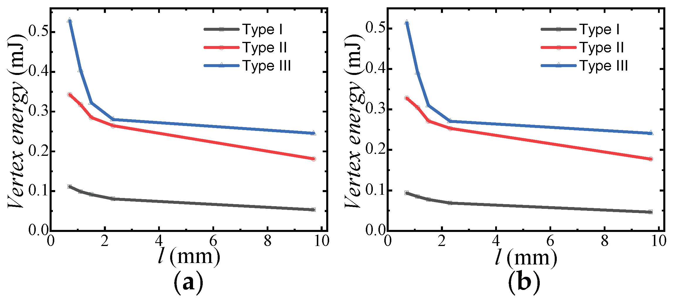
Error estimation: As shown in Extended Figure 1(a), at a positional deviation of -0.1 mm, the vertex energies of the three vertex types slightly increase; conversely, at +0.1 mm in Extended Figure 1(b), they slightly decrease. The energy changes observed in the two panels are nearly identical, with very close numerical values. Taken together, these energy data indicate that the non-monotonic dependence in vertex propositions does not arise from local positional deviations.
Extended Figure 1.
Vertex energies for three vertex types at ±0.1 mm positional deviation. (a) Vertex energies for -0.1 mm positional deviation. (b) Vertex energies for +0.1 mm positional deviation.
Extended Figure 1.
Vertex energies for three vertex types at ±0.1 mm positional deviation. (a) Vertex energies for -0.1 mm positional deviation. (b) Vertex energies for +0.1 mm positional deviation.
Author Contributions
Writing—original draft preparation, J. D. G.; writing—review and editing, J. D. G. The author has read and agreed to the published version of the manuscript.
Funding
This research received no external funding.
Data Availability Statement
The data supporting the findings of this study are available from the corresponding author upon reasonable request.
Conflicts of Interest
The author declares no conflicts of interest.
Abbreviations
The following abbreviations are used in this manuscript:
| AFM | Antiferromagnetic |
| DS | Disordered state |
| PMMA | Polymethyl methacrylate |
| r.l.u. | Reciprocal lattice unit |
| a.u. | Arbitrary unit |
| EO | Excited ordered states |
| SD | Standard deviation |
References
- Arava, H.; Tapia, I.; Cote, T.; et al. Geometry driven intermediate states in artificial square ice structures. Commun. Mater. 2026, 7, 142. [Google Scholar] [CrossRef]
- Pauling, L. The structure and entropy of ice and of other crystals with some randomness of atomic arrangement. J. Am. Chem. Soc. 1935, 57, 2680–2684. [Google Scholar] [CrossRef]
- Lieb, E.H. Exact solution of the problem of the entropy of two-dimensional ice. Phys. Rev. Lett. 1967, 18, 692. [Google Scholar] [CrossRef]
- Lieb, E.H. Residual entropy of square ice. Phys. Rev. 1967, 162, 162–172. [Google Scholar] [CrossRef]
- Bingham, N.S.; Zhang, X.; Ramberger, J.; et al. Collective ferromagnetism of artificial square spin ice. Phys. Rev. Lett. 2022, 129, 067201. [Google Scholar] [CrossRef] [PubMed]
- Coraux, J.; Rougemaille, N. Unusual Coulomb phase physics in the arctic square ice. Phys. Rev. B 2024, 110, 174432. [Google Scholar] [CrossRef]
- Wang, R.F.; Nisoli, C.; Freitas, R.S.; et al. Artificial 'spin ice' in a geometrically frustrated lattice of nanoscale ferromagnetic islands. Nature 2006, 439, 303–306. [Google Scholar] [CrossRef] [PubMed]
- Goryca, M.; Zhang, X.; Watts, J.D.; et al. Magnetic field dependent thermodynamic properties of square and quadrupolar artificial spin ice. Phys. Rev. B 2022, 105, 094406. [Google Scholar] [CrossRef]
- Smith, E.M.; Dudemaine, J.; Placke, B.; et al. Quantum spin ice response to a magnetic field in the dipole-octupole pyrochlore Ce2Zr2O7. Phys. Rev. B 2023, 108, 054438. [Google Scholar] [CrossRef]
- Porée, V.; Yan, H.; Desrochers, F.; et al. Evidence for fractional matter coupled to an emergent gauge field in a quantum spin ice. Nat. Phys. 2025, 21, 83–88. [Google Scholar] [CrossRef]
- Anderson, P.W. Ordering and antiferromagnetism in ferrites. Phys. Rev. 1956, 102, 1008. [Google Scholar] [CrossRef]
- Harris, M.J.; Bramwell, S.T.; McMorrow, D.F.; et al. Geometrical frustration in the ferromagnetic pyrochlore Ho2Ti2O7. Phys. Rev. Lett. 1997, 79, 2554–2557. [Google Scholar] [CrossRef]
- Thompson, C.J. Colouring solutions of the ice problem. J. Stat. Phys. 2011, 145, 647–651. [Google Scholar] [CrossRef]
- Bernal, J.D.; Fowler, R.H. A theory of water and ionic solution, with particular reference to hydrogen and hydroxyl ions. J. Chem. Phys. 1933, 1, 515–548. [Google Scholar] [CrossRef]
- Hu, W.; Zhang, Z.; Liao, Y.; et al. Distinguishing artificial spin ice states using magnetoresistance effect for neuromorphic computing. Nat. Commun. 2023, 14, 2562. [Google Scholar] [CrossRef] [PubMed]
- Yue, W.C.; Yuan, Z.; Huang, P.; et al. Toroidic phase transitions in a direct-kagome artificial spin ice. Nat. Nanotechnol. 2024, 19, 1101–1107. [Google Scholar] [CrossRef] [PubMed]
- Dirac, P.A.M. Quantised singularities in the electromagnetic field. Proc. R. Soc. Lond. A 1931, 133, 60–72. [Google Scholar] [CrossRef]
- Mitsou, V.A. Magnetic Monopoles — From Dirac to the Large Hadron Collider. arXiv 2026, arXiv:2605.02869. [Google Scholar]
- Cao, J.; Kavokin, A. Emergent Magnetic Monopole in Artificial Polariton Spin Ice. arXiv 2026, arXiv:2603.28384. [Google Scholar]
- Puttock, R.; Aandersen, I.M.; Gatel, C.; et al. Defect-induced monopole injection and manipulation in artificial spin ice. Nat. Commun. 2022, 13, 3641. [Google Scholar] [CrossRef] [PubMed]
- Frank, J.; van Lierop, J.; Stamps, R.L. Monopole current control in artificial spin ice via localized fields. Nano Lett. 2025, 25, 12799–12805. [Google Scholar] [CrossRef] [PubMed]
- Duarte, D.G.; De Oliveira, L.B.; Nascimento, F.S.; et al. Magnetic monopole free motion in two-dimensional artificial spin ice. Appl. Phys. Lett. 2024, 124, 112413. [Google Scholar] [CrossRef]
- Fennell, T.; Harris, M.J.; Calder, S.; et al. Multiple Coulomb phase in the fluoride pyrochlore CsNiCrF6. Nat. Phys. 2019, 15, 60–66. [Google Scholar] [CrossRef]
- Giblin, S.R.; Bramwell, S.T.; Holdsworth, P.C.W.; et al. Creation and measurement of long-lived magnetic monopole currents in spin ice. Nat. Phys. 2011, 7, 252–258. [Google Scholar] [CrossRef]
- Castelnovo, C.; Moessner, R.; Sondhi, S.L. Magnetic monopoles in spin ice. Nature 2008, 451, 42–45. [Google Scholar] [CrossRef] [PubMed]
- Pearce, M.J.; Götze, K.; Szabó, A.; et al. Magnetic monopole density and antiferromagnetic domain control in spin-ice iridates. Nat. Commun. 2022, 13, 444. [Google Scholar] [CrossRef] [PubMed]
- Gingras, M.J.P. Observing monopoles in a magnetic analog of ice. Science 2009, 326, 375–376. [Google Scholar] [CrossRef] [PubMed]
- Thonig, D.; Reißaus, S.; Mertig, I.; et al. Thermal string excitations in artificial spin-ice square dipolar arrays. J. Phys. Condens. Matter 2014, 26, 266006. [Google Scholar] [CrossRef] [PubMed]
- Mol, L.A.; Silva, R.L.; Silva, R.C.; et al. Magnetic monopole and string excitations in two-dimensional spin ice. J. Appl. Phys. 2009, 106, 063913. [Google Scholar] [CrossRef]
- Zhang, X.; Duzgun, A.; Lao, Y.; et al. String phase in an artificial spin ice. Nat. Commun. 2021, 12, 6514. [Google Scholar] [CrossRef] [PubMed]
- Mengotti, E.; Heyderman, L.J.; Rodríguez, A.F.; et al. Real-space observation of emergent magnetic monopoles and associated Dirac strings in artificial kagome spin ice. Nat. Phys. 2011, 7, 68–74. [Google Scholar] [CrossRef]
- Skovdal, B.E.; Slöetjes, S.D.; Pohlit, M.; et al. Thermal excitations within and among mesospins in artificial spin ice. Phys. Rev. B 2023, 107, L060406. [Google Scholar] [CrossRef]
- Mondal, A.K.; Barman, A. String phase driven reconfigurable magnonics in Santa Fe ice. Phys. Rev. B 2024, 109, 184433. [Google Scholar] [CrossRef]
- Sivaramakrishnan, A.; Ganesh, R. Ice on curved surfaces: Defect rings and differential local dynamics. Phys. Rev. B 2024, 110, 144202. [Google Scholar] [CrossRef]
- Hull, C.M. Monopoles, Dirac strings and generalised symmetries. J. High Energy Phys. 2025, 2025, 1–32. [Google Scholar] [CrossRef]
- Arava, H.; Vedmedenko, E.Y.; Cui, J.; et al. Control of emergent magnetic monopole currents in artificial spin ice. Phys. Rev. B 2020, 102, 144413. [Google Scholar] [CrossRef]
- Pal, S.; Powell, S. Crossover from string to cluster dynamics following a field quench in spin ice. Phys. Rev. B 2024, 109, 094427. [Google Scholar] [CrossRef]
- Nambu, Y. Strings, monopoles, and gauge fields. Phys. Rev. D 1974, 10, 4262. [Google Scholar] [CrossRef]
- Ojha, B.; Grassi, M.P.; Kapaklis, V. Mapping Reversal Pathways and Interaction Fields in Artificial Spin Ice. arXiv 2026, arXiv:2604.24382. [Google Scholar]
- Jaubert, L.D.C.; Holdsworth, P.C.W. Signature of magnetic monopole and Dirac string dynamics in spin ice. Nat. Phys. 2009, 5, 258–261. [Google Scholar] [CrossRef]
- Zapke, A.H.; Holdsworth, P.C.W. Monopoles, Dirac strings, and magnetic noise in model spin ice. Phys. Rev. Res. 2025, 7, 033284. [Google Scholar] [CrossRef]
- Morris, D.J.P.; Tennant, D.A.; Grigera, S.A.; et al. Dirac strings and magnetic monopoles in the spin ice Dy2Ti2O7. Science 2009, 326, 411–414. [Google Scholar] [CrossRef] [PubMed]
- Mennitl, M.; Leo, N.; Villalba-González, P.; et al. Relaxation pathways and emergence of domains in square artificial spin ice. Phys. Rev. B 2025, 112, 134410. [Google Scholar] [CrossRef]
- Cochran, T.A.; Jobst, B.; Rosenberg, E.; et al. Visualizing dynamics of charges and strings in (2 + 1)D lattice gauge theories. Nature 2025, 642, 315–320. [Google Scholar] [CrossRef] [PubMed]
- Edberg, R.; Khansili, A.; Fjellvåg, I.M.; et al. Magnetic monopole relaxation effects in spin ice Dy2Ti2O7. Phys. Rev. B 2025, 112, 094435. [Google Scholar] [CrossRef]
- Coraux, J.; Rouger, N.; Canals, B.; et al. Square ice Coulomb phase as a percolated vertex lattice. Phys. Rev. B 2024, 109, 224422. [Google Scholar] [CrossRef]
- Perrin, Y.; Canals, B.; Rougemaille, N. Extensive degeneracy, Coulomb phase and magnetic monopoles in artificial square ice. Nature 2016, 540, 410–413. [Google Scholar] [CrossRef] [PubMed]
- Canals, B. Emergence of geometric order from topological constraints in a three-dimensional Coulomb phase. arXiv 2026, arXiv:2602.24051. [Google Scholar]
- Henley, C.L. The "Coulomb phase" in frustrated systems. Annu. Rev. Condens. Matter Phys. 2010, 1, 179–210. [Google Scholar] [CrossRef]
- Borsten, L.; Kim, H. Discrete p-form symmetry and higher Coulomb phases in various theories. Phys. Rev. D. 2026, 113, 125012. [Google Scholar] [CrossRef]
- Huse, D.A.; Krauth, W.; Moessner, R.; et al. Coulomb and liquid dimer models in three dimensions. Phys. Rev. Lett. 2003, 91, 167004. [Google Scholar] [CrossRef] [PubMed]
- Castelnovo, C. Resonant valence bond Coulomb phase: From spins to phonons. Proc. Natl. Acad. Sci. USA 2025, 122, e2506041122. [Google Scholar] [CrossRef] [PubMed]
- Fennell, T.; Deen, P.P.; Wildes, A.R.; et al. Magnetic Coulomb phase in the spin ice Ho2Ti2O7. Science 2009, 326, 415–417. [Google Scholar] [CrossRef] [PubMed]
- Saccone, M.; Van den Berg, A.; Harding, E.; et al. Exploring the phase diagram of 3D artificial spin-ice. Commun. Phys. 2023, 6, 217. [Google Scholar] [CrossRef]
- Rougemaille, N.; Canals, B. Cooperative magnetic phenomena in artificial spin systems: spin liquids, Coulomb phase and fragmentation of magnetism–a colloquium. Eur. Phys. J. B 2019, 92, 62. [Google Scholar] [CrossRef]
- Pandey, J.; Kundu, S.; Damle, K. Z3 confined and deconfined Coulomb liquids in S_eff = 3/2 pyrochlore magnets. arXiv 2026, arXiv:2602.23041. [Google Scholar]
- Jaubert, L.D.C.; Haque, M.; Moessner, R. Analysis of a fully packed loop model arising in a magnetic Coulomb phase. Phys. Rev. Lett. 2011, 107, 177202. [Google Scholar] [CrossRef] [PubMed]
- Lhotel, E.; Leger, M. Spin Dynamics and Unconventional Coulomb Phase in Nd2Zr2O7. In Bulletin of the American Physical Society, APS March Meeting Abstracts; American Physical Society: College Park, MD, USA, 2022; p. T51.007. [Google Scholar]
- Quilliam, J.A.; Yaraskavitch, L.R.; Dabkowska, H.A.; et al. Dynamics of the magnetic susceptibility deep in the Coulomb phase of the dipolar spin ice material Ho2Ti2O7. Phys. Rev. B 2011, 83, 094424. [Google Scholar] [CrossRef]
- Davier, N.; Albarracín, F.G.; Rosales, H.D.; et al. Pinch-line spin liquids as layered Coulomb phases. arXiv 2025, arXiv:2502.16978. [Google Scholar]
- Singh, C.; Arroo, D.M.; Ray, N. Micromagnetic simulations of emergent monopole defects and magnetization reversal in connected and dipolar Square Artificial Spin Ice. J. Magn. Magn. Mater. 2024, 594, 171887. [Google Scholar] [CrossRef]
- Jaubert, L.D.C.; Chalker, J.T.; Holdsworth, P.C.W.; et al. Three-dimensional Kasteleyn transition: Spin ice in a [100] field. Phys. Rev. Lett. 2008, 100, 067207. [Google Scholar] [CrossRef] [PubMed]
- Pal, S.; Powell, S. Dynamic scaling near the Kasteleyn transition in spin ice: critical relaxation of monopoles and strings following a field quench. Phys. Rev. B 2026, 114, 024402. [Google Scholar] [CrossRef]
- Kasteleyn, P.W. The statistics of dimers on a lattice: I. The number of dimer arrangements on a quadratic lattice. Physica 1961, 27, 1209–1225. [Google Scholar]
- Potts, M.; Benton, O. Spin ice in a general applied magnetic field: Kasteleyn transition, magnetic torque, and rotational magnetocaloric effect. Phys. Rev. B 2022, 106, 054437. [Google Scholar] [CrossRef]
- Kasteleyn, P.W. Dimer statistics and phase transitions. J. Math. Phys. 1963, 4, 287–293. [Google Scholar] [CrossRef]
- Powell, S. Quantum Kasteleyn transition. Phys. Rev. B 2022, 105, 064413. [Google Scholar] [CrossRef]
- Baez, M.L.; Borzi, R.A. The 3D Kasteleyn transition in dipolar spin ice: a numerical study with the conserved monopoles algorithm. J. Phys. Condens. Matter 2017, 29, 055806. [Google Scholar] [CrossRef] [PubMed]
- Karlova, K.; Rufino, A.; Verkhol, Y.T.; et al. Approaching Kasteleyn transition in frustrated quantum Heisenberg antiferromagnets. arXiv 2026, arXiv:2601.14382. [Google Scholar]
- Pili, L.; Steppke, A.; Barber, M.E.; et al. Topological metamagnetism: Thermodynamics and dynamics of the transition in spin ice under uniaxial compression. Phys. Rev. B 2022, 105, 184422. [Google Scholar] [CrossRef]
- Fennell, T.; Bramwell, S.T.; McMorrow, D.F.; et al. Pinch points and Kasteleyn transitions in kagome ice. Nat. Phys. 2007, 3, 566–572. [Google Scholar] [CrossRef]
- Oliveira, G.A.; Moura-Melo, W.A.; Pereira, A.R.; et al. Energetics and thermodynamics of bilayer rectangular artificial spin ices. J. Magn. Magn. Mater. 2026, 639, 173753. [Google Scholar] [CrossRef]
- Peroor, R.R.; Scafuri, L.A.; Bozhko, D.A.; et al. Frequency comb in a macroscopic mechanomagnetic artificial spin ice. Phys. Rev. Appl. 2025, 23, 044010. [Google Scholar] [CrossRef]
- Mellado, P.; Concha, A.; Mahadevan, L. Macroscopic magnetic frustration. Phys. Rev. Lett. 2012, 109, 257203. [Google Scholar] [CrossRef] [PubMed]
- Scafuri, L.A.; Bozko, D.A.; Iacocca, E. Wave dynamics in a macroscopic square artificial spin ice. Phys. Rev. Appl. 2025, 23, 054093. [Google Scholar] [CrossRef]
- Farhan, A.; Saccone, M.; Petersen, C.F.; et al. Emergent magnetic monopole dynamics in macroscopically degenerate artificial spin ice. Sci. Adv. 2019, 5, eaav6380. [Google Scholar] [CrossRef] [PubMed]
- Teixeira, H.A.; Bernardo, M.F.; Nascimento, F.S.; et al. Macroscopic magnetic monopoles in a 3D-printed mechano-magnet. J. Magn. Magn. Mater. 2024, 596, 171929. [Google Scholar] [CrossRef]
- Gonçalves, R.S.; Gomes, A.C.C.; Loreto, R.P.; et al. Naked-eye visualization of geometric frustration effects in macroscopic spin ices. J. Magn. Magn. Mater. 2020, 502, 166471. [Google Scholar] [CrossRef]
- Wang, K.; Liu, X.J.; Tu, L.M.; et al. Experimental realization of the ground state for the antiferromagnetic Ising model on a triangular lattice. arXiv 2025, arXiv:2501.10026. [Google Scholar]
- Cisternas, J.; Navarro, M.; Duarte, S.; et al. Equilibrium and symmetries of altitudinal magnetic rotors on a circle. Chaos 2022, 32, 123120. [Google Scholar] [CrossRef] [PubMed]
- Ge, J.Y.; Zhang, J.J.; Tu, L.M.; et al. Growing crystalline artificial kagome ice at the macroscale. Newton 2025, 1, 100143. [Google Scholar] [CrossRef]
- Matsunaga, D.; Hamilton, J.K.; Meng, F.; et al. Controlling collective rotational patterns of magnetic rotors. Nat. Commun. 2019, 10, 4696. [Google Scholar] [CrossRef] [PubMed]
- Maes, J.; De Gusem, D.; Lateur, I.; et al. The design, verification, and applications of Hotspice: a Monte Carlo simulator for artificial spin ice. Comput. Phys. Commun. 2025, 313, 109643. [Google Scholar] [CrossRef]
Figure 1.
Sample structure and two ground states of a unit.. (a) Schematic of a sample for macroscopic square ice. (b) Leftward pseudospin. The bold arrow denotes the pseudospin. The parameter l is the unit gap. (c) Rightward pseudospin. (d) Variation of unit energy as a function of l for different values of Z.
Figure 1.
Sample structure and two ground states of a unit.. (a) Schematic of a sample for macroscopic square ice. (b) Leftward pseudospin. The bold arrow denotes the pseudospin. The parameter l is the unit gap. (c) Rightward pseudospin. (d) Variation of unit energy as a function of l for different values of Z.
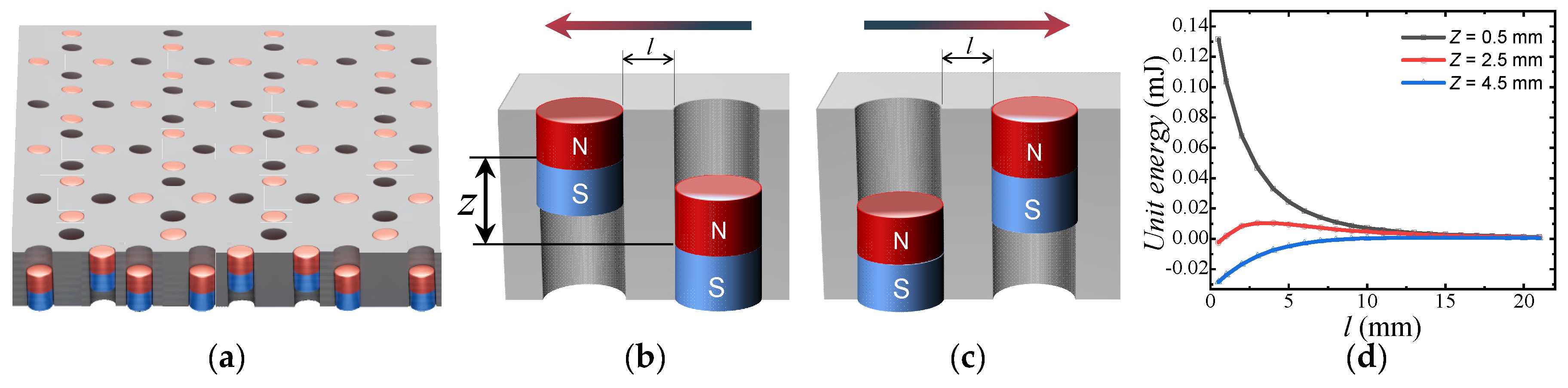
Figure 3.
Sample assembly method in macroscopic square ice. (a) Magnet order of horizontal units. (b) Magnet order of vertical units. (c) Vertex energy for three types of vertices.
Figure 3.
Sample assembly method in macroscopic square ice. (a) Magnet order of horizontal units. (b) Magnet order of vertical units. (c) Vertex energy for three types of vertices.
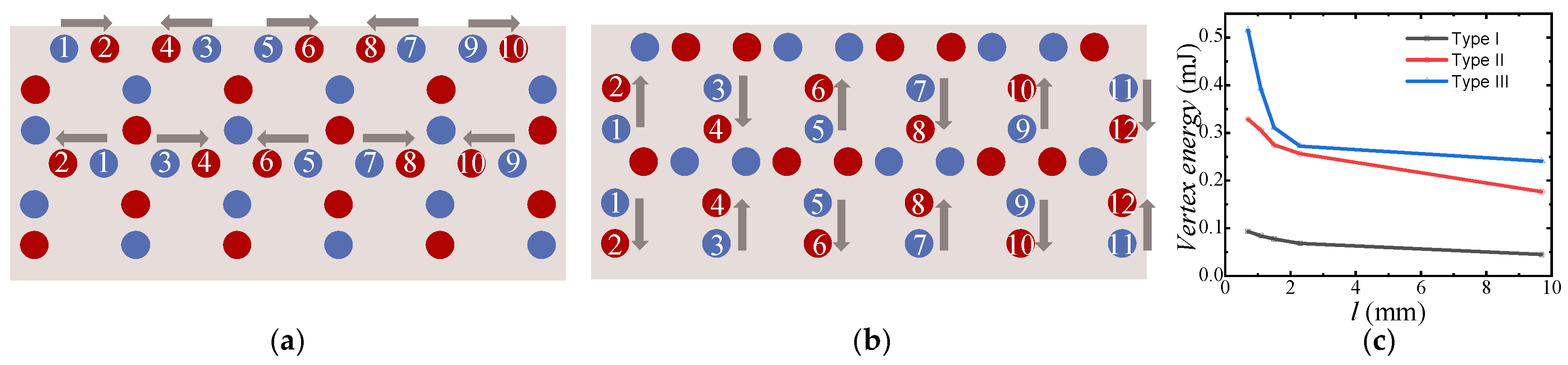
Figure 4.
Traps structures and magnets used in macroscopic square ice. (a) Trap diameter D′. (b) Distribution of trap diameter D′. (c) Magnets with two different heights. (d) Distribution of magnet diameter D.
Figure 4.
Traps structures and magnets used in macroscopic square ice. (a) Trap diameter D′. (b) Distribution of trap diameter D′. (c) Magnets with two different heights. (d) Distribution of magnet diameter D.
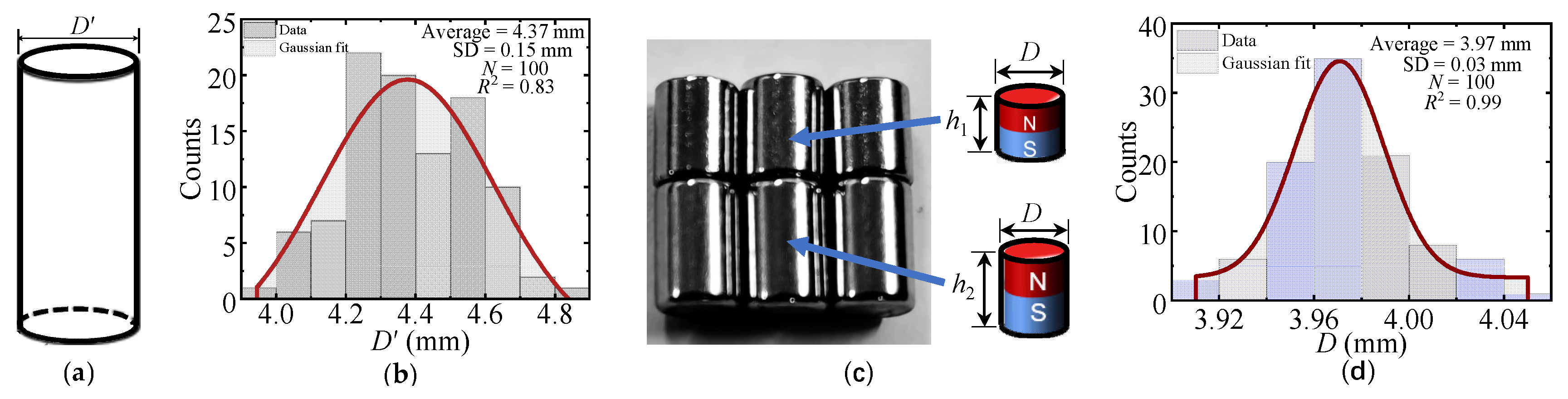
Figure 5.
Distributions of measured parameters for short magnets. (a) Distribution of magnetic flux density B1. (b) Distribution of mass m1. (c) Distribution of height h1.
Figure 5.
Distributions of measured parameters for short magnets. (a) Distribution of magnetic flux density B1. (b) Distribution of mass m1. (c) Distribution of height h1.
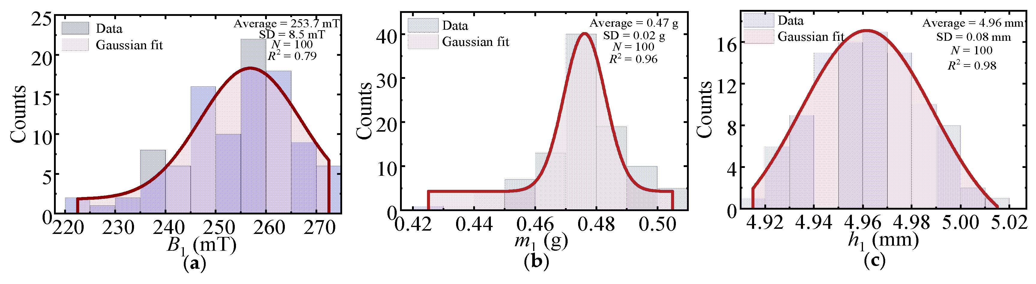
Figure 6.
Distributions of measured parameters for long magnets. (a) Distribution of magnetic flux density B2. (b) Distribution of mass m2. (c) Distribution of height h2.
Figure 6.
Distributions of measured parameters for long magnets. (a) Distribution of magnetic flux density B2. (b) Distribution of mass m2. (c) Distribution of height h2.
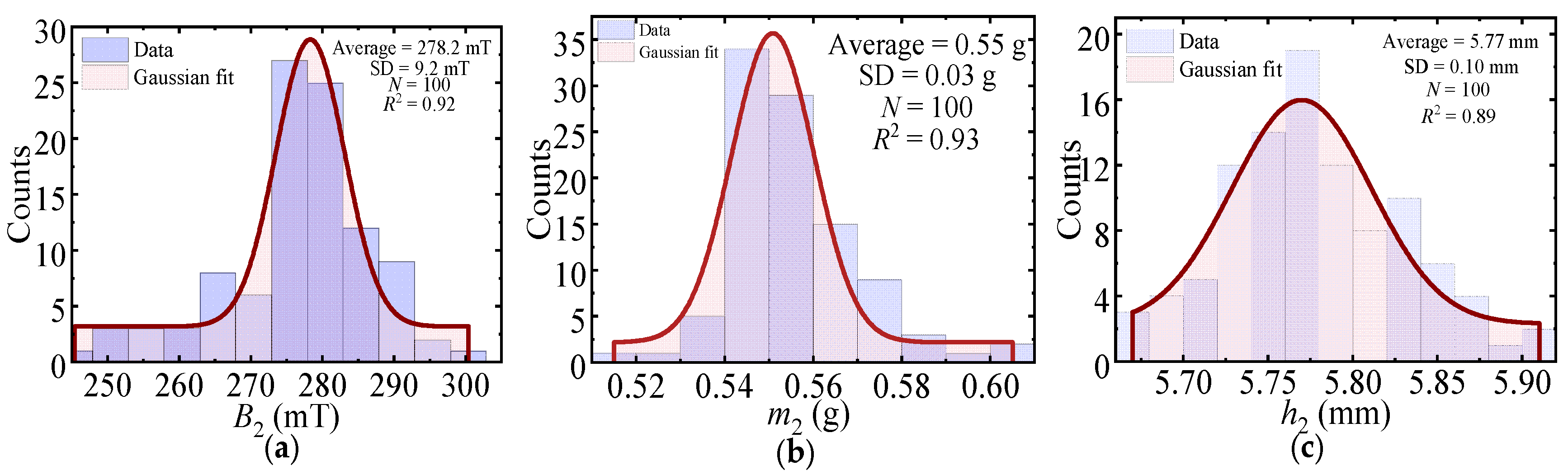
Figure 7.
Ordering states of macroscopic square ice. (a) Excited ordered state. (b) Antiferromagnetic ordered state. (c) Disordered state. (d) Antiferromagnetic ordered state.
Figure 7.
Ordering states of macroscopic square ice. (a) Excited ordered state. (b) Antiferromagnetic ordered state. (c) Disordered state. (d) Antiferromagnetic ordered state.
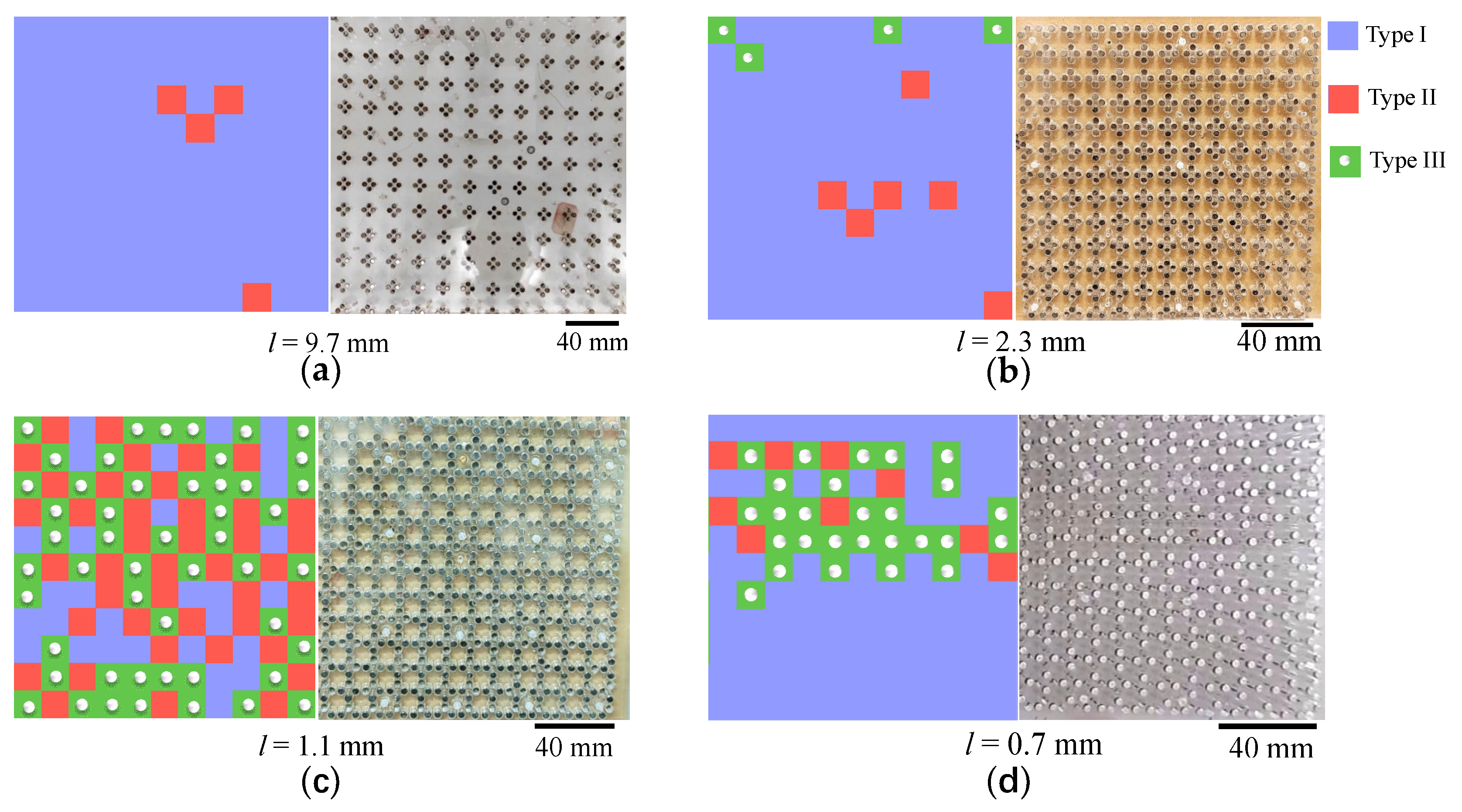
Figure 8.
States, correlations, and unit proportions of macroscopic square ice. (a) States and vertex proportions. (b) Correlation functions of nearest-neighbor I and the next-nearest-neighbor L. (c) Unit proportions for different types of units.
Figure 8.
States, correlations, and unit proportions of macroscopic square ice. (a) States and vertex proportions. (b) Correlation functions of nearest-neighbor I and the next-nearest-neighbor L. (c) Unit proportions for different types of units.
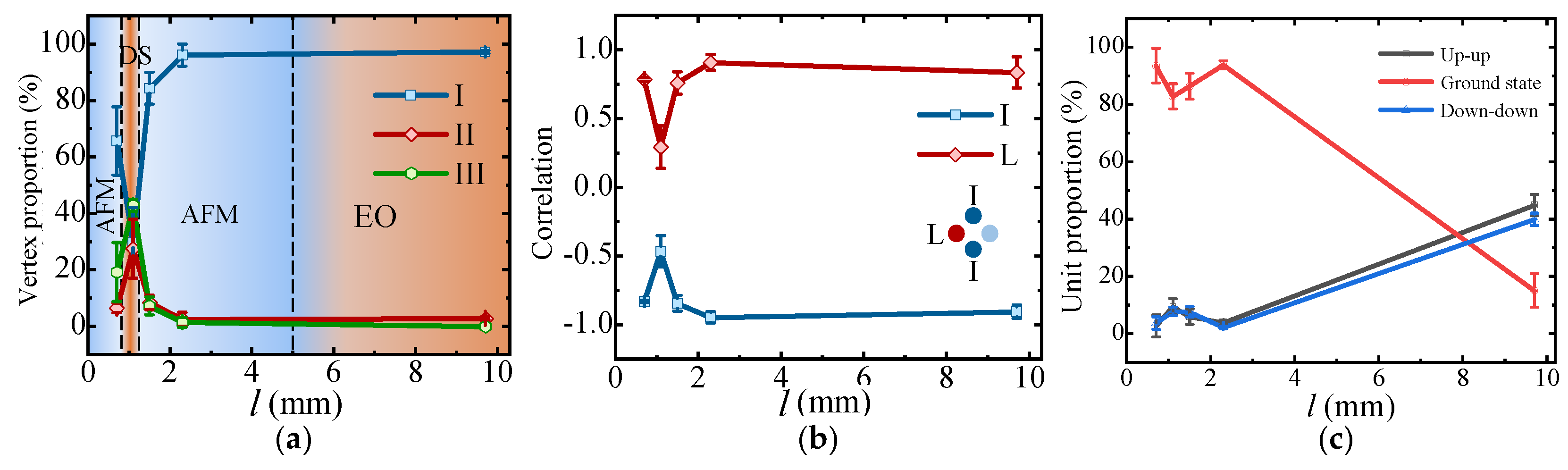
Figure 9.
Magnetic structure factors of macroscopic square ice. (a) Antiferromagnetic states for l = 1.5 mm. (b) Disordered states for l = 1.1 mm. (c) Antiferromagnetic states for l = 0.7 mm.
Figure 9.
Magnetic structure factors of macroscopic square ice. (a) Antiferromagnetic states for l = 1.5 mm. (b) Disordered states for l = 1.1 mm. (c) Antiferromagnetic states for l = 0.7 mm.
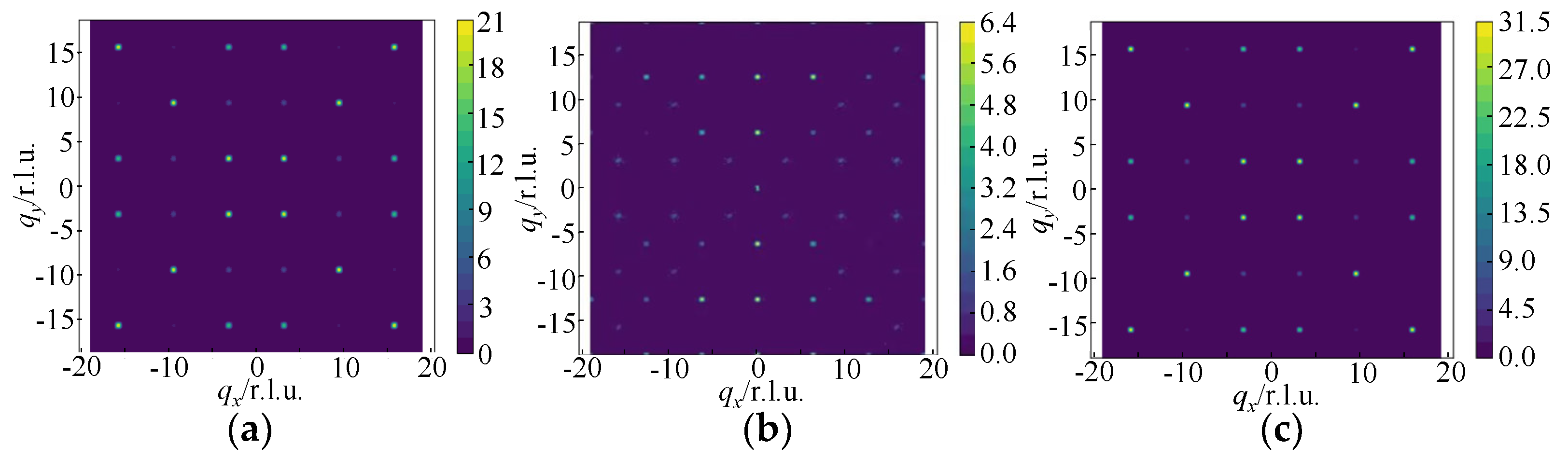

Table 1.
Parameters of traps and short magnets.
| Properties | Trap diameter D′ | Magnetic flux density B1 | Diameter D | Mass m1 | Height h1 |
|---|---|---|---|---|---|
| Average | 4.37 mm | 253.7 mT | 3.97 mm | 0.47 g | 4.96 mm |
| Standard deviation | ±0.15 mm | ±8.5 mT | ±0.03 mm | ±0.02 g | ±0.08 mm |
Table 2.
Parameters of long magnets.
| Properties | Magnetic flux density B2 | Diameter D | Mass m2 | Height h2 |
|---|---|---|---|---|
| Average | 278.2 mT | 3.97 mm | 0.55 g | 5.77 mm |
| Standard deviation | ±9.2 mT | ±0.03 mm | ±0.03 g | ±0.10 mm |
Table 3.
Statistics of Type-I vertices.
| Unit gap l | Sample 1 | Sample 2 | Sample 3 | Mean values | Standard deviations |
|---|---|---|---|---|---|
| 9.7 mm | 118 (97.52%) | 106 (87.60%) | 105 (86.78%) | 109.66 (90.63%) | 7.24 (5.98%) |
| 2.3 mm | 120 (99.17%) | 118 (97.52%) | 111 (91.74%) | 116.33 (96.14%) | 4.73 (3.91%) |
| 1.5 mm | 84 (69.42%) | 111 (91.74%) | 108 (89.26%) | 101 (83.47%) | 14.80 (12.23%) |
| 1.1 mm | 29 (23.97%) | 43 (35.31%) | 60 (49.59%) | 44 (36.36%) | 15.52 (12.83%) |
| 0.7 mm | 106 (87.60%) | 95 (78.51%) | 85 (70.25%) | 95.33 (78.79%) | 10.50 (8.68%) |
Table 4.
Statistics of Type-II vertices.
| Unit gap l | Sample 1 | Sample 2 | Sample 3 | Mean values | Standard deviations |
|---|---|---|---|---|---|
| 9.7 mm | 3 (2.48%) | 12 (9.92%) | 15 (12.40%) | 10 (8.26%) | 6.24 (5.16%) |
| 2.3 mm | 0 (0%) | 3 (2.48%) | 6 (4.96%) | 3 (2.48%) | 3 (2.48%) |
| 1.5 mm | 21 (17.36%) | 4 (3.31%) | 4 (3.31%) | 9.67 (7.99%) | 9.81 (8.11%) |
| 1.1 mm | 42 (34.71%) | 27 (22.31%) | 20 (16.53%) | 29.67 (24.52%) | 11.24 (9.29%) |
| 0.7 mm | 9 (7.44%) | 7 (5.79%) | 9 (7.44%) | 8.33 (6.89%) | 1.15 (0.95%) |
Table 5.
Statistics of Type-III vertices.
| Unit gap l | Sample 1 | Sample 2 | Sample 3 | Mean values | Standard deviations |
|---|---|---|---|---|---|
| 9.7 mm | 0 (0%) | 3 (2.48%) | 1 (0.83%) | 1.33 (1.11%) | 1.52 (1.26%) |
| 2.3 mm | 1 (0.83%) | 0 (0%) | 4 (3.31%) | 1.67 (1.38%) | 2.08 (1.72%) |
| 1.5 mm | 16 (13.22%) | 6 (4.96%) | 9 (7.44%) | 10.33 (8.54%) | 5.13 (4.24%) |
| 1.1 mm | 50 (41.32%) | 51 (42.15%) | 41 (33.88%) | 47.33 (39.12%) | 5.51 (4.55%) |
| 0.7 mm | 9 (7.44%) | 19 (15.70%) | 27 (22.31%) | 18.33 (15.15%) | 9.02 (7.45%) |
Table 6.
Maximal size (number of vertices) of a single domain.
| Unit gap l | Type-I domain | Type-II domain | Type-III domain | Total number of vertices |
|---|---|---|---|---|
| 9.7 mm | 118 (97.52%) | 1 (0.83%) | 0 (0%) | 121 (100%) |
| 2.3 mm | 118 (97.52%) | 1 (0.83%) | 1 (0.83%) | 121 (100%) |
| 1.5 mm | 119 (98.35%) | 3 (2.48%) | 2 (1.65%) | 121 (100%) |
| 1.1 mm | 30 (24.79%) | 4 (3.31%) | 15 (12.40%) | 121 (100%) |
| 0.7 mm | 68 (56.20%) | 5 (4.13%) | 17 (14.05%) | 121 (100%) |
Table 7.
Distribution of Type-I magnetic domain sizes and the mean domain size.
| Unit gap l | [0, 20) | [20, 40) | [40, 60) | [60, 80) | [80, 100) | [100, 120] | Mean size |
|---|---|---|---|---|---|---|---|
| 9.7 mm | 0 | 0 | 0 | 0 | 0 | 3 | 108 |
| 2.3 mm | 0 | 0 | 0 | 0 | 0 | 3 | 114.5 |
| 1.5 mm | 9 | 1 | 0 | 0 | 0 | 3 | 12 |
| 1.1 mm | 18 | 1 | 0 | 0 | 0 | 0 | 3.4 |
| 0.7 mm | 3 | 1 | 0 | 1 | 0 | 0 | 22 |
Table 8.
Distribution of Type-II magnetic domain sizes and the mean domain size.
| Unit gap l | [1, 2) | [2, 3) | [3, 4) | [4, 5) | [5, 6) | Mean size |
|---|---|---|---|---|---|---|
| 9.7 mm | 17 | 0 | 0 | 0 | 0 | 1 |
| 2.3 mm | 9 | 0 | 0 | 0 | 0 | 1 |
| 1.5 mm | 28 | 3 | 1 | 0 | 0 | 1.2 |
| 1.1 mm | 24 | 1 | 1 | 1 | 0 | 1.2 |
| 0.7 mm | 10 | 0 | 0 | 1 | 1 | 1.6 |
Table 9.
Distribution of Type-III magnetic domain sizes and the mean domain size.
| Unit gap l | (0, 2) | [2, 4) | [4, 6) | [6, 8) | [8, 10) | [10, 12) | [12, 14) | [14, 16) | [16, 18) | Mean size |
|---|---|---|---|---|---|---|---|---|---|---|
| 9.7 mm | 0 | 0 | 0 | 0 | 0 | 0 | 0 | 0 | 0 | 0 |
| 2.3 mm | 9 | 0 | 0 | 0 | 0 | 0 | 0 | 0 | 0 | 1 |
| 1.5 mm | 25 | 4 | 0 | 0 | 0 | 0 | 0 | 0 | 0 | 1.2 |
| 1.1 mm | 20 | 4 | 1 | 0 | 0 | 1 | 1 | 1 | 0 | 2.6 |
| 0.7 mm | 7 | 3 | 1 | 1 | 0 | 0 | 0 | 0 | 1 | 3.2 |
Disclaimer/Publisher’s Note: The statements, opinions and data contained in all publications are solely those of the individual author(s) and contributor(s) and not of MDPI and/or the editor(s). MDPI and/or the editor(s) disclaim responsibility for any injury to people or property resulting from any ideas, methods, instructions or products referred to in the content. |
© 2026 by the author. Licensee MDPI, Basel, Switzerland. This article is an open access article distributed under the terms and conditions of the Creative Commons Attribution (CC BY) license.
Copyright: This open access article is published under a Creative Commons CC BY 4.0 license, which permit the free download, distribution, and reuse, provided that the author and preprint are cited in any reuse.