

Submitted:
25 August 2026
Posted:
27 August 2026
You are already at the latest version
Abstract
Reliable prediction of the El Niño–Southern Oscillation (ENSO) at multi-year lead times remains challenging because forecast skill generally declines beyond 12–18 months. This study presents a streamlined Informer-based framework designed to predict the Niño 3.4 index up to 36 months in advance using one-dimensional climate time series. The proposed model was developed following an analysis of the earlier Multimodal ENSO Forecast framework, which showed that most of the long-lead predictive skill originated from the time-series branch, whereas the spatial branch added substantial computational cost with limited benefit. Historical simulations from CMIP5 and selected CMIP6 models were used for training, followed by calibration with GODAS observations from 1980 to 2000 and independent validation over 2001–2020. The model achieved anomaly correlation coefficient values of 0.92, 0.75, 0.56, 0.46, 0.48, and 0.41 at lead times of 1, 6, 12, 18, 24, and 30 months, respectively. At directly comparable lead times, its performance was consistently higher than that of the CNN benchmark, with the largest difference observed at 18 months. The model also maintained useful predictive skill at extended lead times and showed reduced sensitivity to the spring predictability barrier. In addition, the simplified architecture required substantially less computational effort than the original multimodal framework and supported inference on a standard CPU. These results demonstrate that an efficiently optimized time-series architecture, combined with climate-model-based data augmentation, can provide competitive and computationally practical ENSO forecasts at multi-year horizons.
Keywords:
ENSO forecasting
; informer
; long-lead prediction
; CMIP5/CMIP6
; time series forecasting
; deep learning
1. Introduction
The El Niño–Southern Oscillation (ENSO) is a major mode of coupled ocean–atmosphere variability and one of the most important sources of interannual climate fluctuations. It is mainly expressed through anomalous sea surface temperature variations in the tropical Pacific Ocean and associated changes in atmospheric circulation. ENSO events, including the warm El Niño phase and the cold La Niña phase, have generally been described as irregular phenomena occurring at intervals of about 2 to 7 years (Wang et al. 2023). Recent observations, however, suggest that ENSO variability may be changing under the influence of a warming climate. In particular, Central Pacific El Niño events have occurred more frequently since 2000, and their dominant recurrence period has shortened from approximately 4–5 years to 2–3 years (Jia and Guo 2025). This change points to a less stationary ENSO regime and highlights the need for forecasting methods that can remain reliable under evolving climate conditions.
The practical importance of ENSO prediction has also become more evident in recent years. The strong 2023–2024 El Niño event, together with record greenhouse gas concentrations and other contributing factors, contributed to the exceptional warmth of 2024, which was confirmed as the warmest year on record (WMO 2025). In addition, the World Meteorological Organization reported an 80% likelihood of El Niño conditions during June–August 2026, with probabilities near or above 90% for continuation until at least November 2026 (WMO 2026a). Recent European heat extremes further underline the practical value of improved climate early-warning systems. Europe experienced severe heatwave conditions in 2025, and the late-June 2026 heatwave broke numerous temperature records while affecting human health, ecosystems, agriculture, infrastructure, and labour productivity (WMO 2026b; WMO 2026c). According to the World Meteorological Organization, more than 1,300 excess deaths had been recorded across Europe since 21 June in association with the extreme heat, while preliminary national mortality estimates later indicated at least 3,700 excess deaths during the June heatwave in France, Belgium, and the Netherlands alone (WMO 2026d; Reuters 2026). Although European heatwaves cannot be attributed to ENSO alone, ENSO-related teleconnections can influence atmospheric circulation and climate anomalies outside the tropical Pacific. Therefore, improving long-term ENSO forecasting is essential for climate-risk preparedness and for decision-making in agriculture, water-resource management, disaster-risk reduction, public health, and energy planning (Scaife 2010; Blöschl et al. 2019; L’Heureux et al. 2020).
The use of machine learning has introduced new methods to address these long-standing problems.
However, current dynamic forecasting models continue to be incapable of providing reliable forecasts greater than a single year; thus, predicting ENSO events for multiple years remains a challenge.
Despite the difficulties that still exist; it has been possible to identify periodic variations and regular cycles associated with the ENSO phenomenon as well as gradual changes in oceanic variability which indicate that the ENSO phenomenon is potentially predictable (Luo et al. 2008).
Anomalies in the equatorial Pacific Ocean associated with several of the recent La Niña events have shown extended time periods of relatively low activity, indicating a change in the ENSO paradigm (Gao and Zhang 2017) that makes it more difficult to make accurate forecasts today compared with the forecast skill seen in the 1980s and 1990s.
By leveraging the potential of machine learning and integrating recent discoveries regarding the teleconnections of the El Niño–Southern Oscillation (ENSO) with other oceanic systems, it is feasible to develop a model capable of forecasting ENSO events beyond a one-year timeframe (Park et al. 2017). Sea Surface Temperature (SST) anomalies occurring outside the equatorial Pacific can indeed signal the onset of ENSO events more than a year in advance. Concurrently, advanced large-scale numerical models have been developed and implemented to elucidate the determinants of Earth's historical climate, thereby enhancing our capacity to predict future climatic conditions (Kirtman and Power 2013). While there is a relatively strong consensus among climate models concerning large-scale temperature signals, uncertainties surrounding dynamical alterations in atmospheric circulation remain significant. This discrepancy inevitably undermines the reliability of long-term forecasts, particularly concerning precipitation projections for the coming decades (Shepherd 2014).
The Multimodal ENSO Forecast (MEF), introduced in our previous work and subsequently evaluated in related studies (Naisipour et al. 2024, 2025a, 2026), combines spatiotemporal oceanic fields with a time-series Informer module to predict ENSO up to 24 months ahead.
Subsequent analysis using ablation revealed that the model's long-range predictive skill (particularly for periods greater than 18 months) was driven almost entirely by the time-series branch through an Informer-based architecture. By comparison, the contribution of high-dimensional spatial input was minimal while imposing considerable computational expense on the model. This finding illustrates that when predicting ENSO beyond 18-month lead times, temporal dynamics provide stronger predictive signals than high-dimensional spatial anomaly patterns, supporting a transition away from multi-modal architectures to time-series-only architectures.
Based on these findings, we propose a more efficient forecasting framework that eliminates unnecessary spatial processing and focuses on one-dimensional climate time-series signals. The Informer architecture (Zhou et al., 2021) is great for doing this since it was created to predict time series of long sequences using an attention mechanism called ProbSparse Self-Attention. This attention method gives more emphasis on the time steps which are important by using their locations and attention weights to make its decisions. The Informer can capture short-term auto-correlations as well as multi-year periodicity in the ENSO time-series without needing to do a lot of feature engineering and without having to find prior clues from outside the model. This extensive dataset allows the deep learning model to learn from a wide range of scenarios, improving its predictive performance.
To enhance the model’s ability to learn ENSO dynamics under different climate backgrounds, we expanded the training dataset by combining historical simulations from CMIP5 and selected CMIP6 models with observational records. Unlike a simple inclusion of all available simulations, the CMIP6 models were screened based on their ability to reproduce key ENSO characteristics, including Niño 3.4 variability, dominant periodicity, seasonal phase locking, and the observed tendency toward more frequent Central Pacific El Niño events after 2000. This selection strategy is consistent with recent model-evaluation studies showing that ENSO-related metrics can be used to diagnose the suitability of coupled climate models for ENSO analysis and prediction (Planton et al. 2021; Jia and Guo 2025). By incorporating CMIP6 simulations that better represent ENSO frequency and variability, the training set covers a broader range of physically plausible ENSO regimes and improves the model’s generalization to the post-2000 climate period.
The model was then retrained and calibrated using Global Ocean Data Assimilation System (GODAS) observations from 1980 to 2000.
The proposed streamlined framework provides several advantages compared with traditional 3D convolutional neural networks (3DCNNs) and other spatially intensive deep-learning approaches. By removing the 3DCNN component from the architecture, the model substantially reduces computational demand and can perform inference without GPU acceleration. This simplified design also eliminates the need to preprocess and store large spatial anomaly maps, reducing both storage requirements and data-management costs. In addition, the modified architecture contains fewer hyperparameters, which makes systematic optimization easier and reduces the risk of overfitting when working with climate datasets that have limited independent sample sizes.
Similarly, in time series forecasting, multimodal techniques have been employed to analyze heterogeneous data streams, such as meteorological and hydrological indicators, to enhance predictive performance. Kumshe et al. (2024) leveraged CNN-LSTM pipeline to capture spatio-temporal data for forecasting hydrological phenomena. In climate science, recent studies have prioritized the prediction of the ENSO through the utilization of spatio-temporal data. Zhao et al. (2023) applied a deep learning model that integrates satellite imagery and oceanographic temporal data, capturing the intricate interactions that influence ENSO events and resulting in notable improvements in prediction skill. Jonnalagadda and Hashemi (2023) explored the use of recurrent neural networks to enhance the prediction of El Niño and La Niña events by optimizing the spatial-temporal extent of environmental factors, demonstrating the potential of advanced modeling techniques in improving climate predictions.
For quantitative benchmarking, we compare our proposed model against two established references: the SINTEX-F dynamical model (Doi et al. 2019) and the CNN-based model of Ham et al. (2019). The benchmark to quantitatively compare our model with regards to performance of forecasting the ENSO is based on the Convolutional Neural Network developed by Ham et al. (2019), which is recognized widely as being one of the best currently available deep-learning predictive models of ENSO. The Ham et al. model uses as input a map of sea surface temperature (SST) and a map showing deviations in ocean heat content (HC), and applies three (2D) convolutional layers in order to derive spatially based features in order to predict the Niño 3.4 index. Although the Ham et al. predictive model has exhibited skill that exceeds the SINTEX-F (Doi et al., 2019) model during the periods covered by these models, (i.e., lead times less than 18 months), the performance of the model (prediction capabilities) greatly diminishes at lead times beyond 18 months when the model's correlation coefficient would be less than 0.50. Most importantly, Ham et al. (2019) model produced poor predictive accuracy for the time period after year 2000. The relationship between the increased frequency of ENSO and the diminished number of spatially reliable "precursory pattern" for the ENSO means that there will be less reliable predictions of the ENSO based on the use of static spatial pattern features. Therein lies a strong argument to explore alternative architectural designs that require less spatially static (i.e., based on using a reliable static feature space) and instead rely extensively on the use of more reliable temporal dynamic relationship to predict the ENSO.
Ham et al. addressed the spring predictability barrier by introducing the ACNN method, a variant of the conventional Convolutional Neural Network (CNN) approach, which incorporates modifications to the architectural design; nevertheless, the overall correlation skill remained consistent (Ham et al. 2021). Zhou et al. posited that by employing the Principal Oscillation Pattern analysis in conjunction with CNN-Long Short-Term Memory (LSTM) (Muhammad et al. 2023) techniques, they could predict the Niño 3.4 index for up to 17 months during the validation period spanning from 1994 to 2017 (Zhou and Zhang 2022). Moreover, Zhou and Zhang (2023) proposed an innovative application of the Transformer architecture, termed 3D-Geoformer, designed for spatiotemporal multivariate predictions of ENSO. This model integrates sea surface zonal and meridional wind stress alongside seven-layer ocean temperature anomalies within the upper 150 meters, employing a three-dimensional framework. The 3D-Geoformer effectively hindcasts the Niño 3.4 index with a lead time of up to 18 months, utilizing data from 1983 to 2021. However, it is important to note that the model yields valid results only for predictions made up to 16 months in advance during the boreal spring. In comparative analyses, the performance of the 3D-Geoformer model was evaluated against that of the CNN model for the period from 1983 to 2017, revealing only marginal improvements in overall forecast skill. Similar to the CNN model, the skill of the 3D-Geoformer post-2000 is relatively low, with its correlation coefficient declining below 0.5 for lead times extending to 13 months.
Recent studies published in high-impact journals have further emphasized the rapid development of hybrid, Transformer-based, and physically informed deep-learning approaches for ENSO prediction. For example, Mu et al. (2024) introduced ENSO-PhyNet, a Transformer-based model that incorporates heat-budget dynamics into self-attention computations to improve physical interpretability. Chen et al. (2025) proposed a combined dynamical–deep learning framework, showing that deep learning can complement dynamical forecast systems and improve ENSO prediction skill. More recently, Zhou et al. (2026) demonstrated that explicitly accounting for tropical basin interactions can reduce the spring predictability barrier and extend effective ENSO prediction beyond 16 months. These studies confirm the growing importance of physically informed and hybrid deep-learning frameworks, while also showing that reliable prediction beyond about 18–24 months remains a major challenge.
Collectively, these advancements highlight the potential of multimodal deep learning approaches to significantly enhance the understanding and prediction of ENSO phenomena, thereby contributing to more effective climate monitoring and response strategies. Despite these advancements, achieving a correlation skill greater than 50% in predicting ENSO events beyond a 12-month horizon continues to pose significant challenges. Given the increasing variability of ENSO, no existing methodology has demonstrated the capacity to predict ENSO occurrences with reliable accuracy at a lead time of 1.5 years.
The increasing impact of climate change upon the dynamics of ENSO leads to more frequent occurrences of extreme El Niño and La Niña phenomenon (Cai et al. 2014, 2020). The evolution of ENSOs’ behaviour under non-stationary climate conditions presents complications for prediction capabilities using traditional modelling techniques, including both dynamical and statistical modelling processes. The inadequate accuracy of predictions has considerable societal repercussions, such as negative effects on agricultural output, management of water resources, and preparation for disaster (L'Heureux et al. 2020). Due to these factors, there is an urgent need to develop new forecasting frameworks capable of predicting changing climate systems; currently existing static spatial precursor patterns may not be applicable to future post-2000 climatic conditions.
The article by Ricke and Caldeira (2014) examines the interplay between natural climate variability, particularly the ENSO, and human-induced climate change, highlighting ENSO's significant role in influencing global weather patterns and climate extremes. The authors underscore the critical importance of accurately distinguishing between the effects of natural variability and those of anthropogenic climate change for effective climate predictions and policies. Consequently, they advocate for further research to enhance our understanding of these dynamics, which is paramount for refining climate models and predicting the ENSO phenomena in the new millennia. In this study, the post-2000 period was chosen exclusively for validation due to the observed increase in the frequency of central Pacific El Niño events and the associated weakening of warm water volume variations, which have complicated ENSO predictions (Guan and McPhaden 2016; Wang et al. 2024). To address this challenge, we developed the enhanced Informer-based forecasting framework described in this paper.
The improved framework presents four substantial contributions. Our first contribution demonstrates the effectiveness of a time-series-only deep learning model that outperforms the existing state of the art with lead times of 36 months (the current state of the art is unable to perform well beyond 18 months). Our second contribution has shown that combining historical data from all CMIP5 and CMIP6 models leads to significantly improved long-lead forecasting skill than if training on only CMIP5 or limited historical observations, therefore providing a way to augment climate forecasting data with historical data. Our third contribution provides a new understanding from an ablation analysis that the high-dimensional spatial input to the model has virtually no impact in forecasting skill beyond 18 months, contrary to previous beliefs that long-term forecast skill required the inclusion of high spatial complexity. Our fourth contribution establishes an entirely new efficient benchmark for operational long-lead ENSO forecasting and shows that an optimized Informer-type forecasting model using only one-dimensional climate data is superior to far more complex and computationally intensive forecasting techniques, such as numerical dynamic models and deep learning techniques that use image data. Together, these contributions redefine the state of the art in long-lead ENSO prediction and offer a replicable framework for extending time-series-based forecasting to other climate phenomena exhibiting multi-year variability.
2. Method
The single streamlined module of the enhanced Time Series Informer (TSI) network is the proposed ENSO forecasting framework. In contrast to our Multimodal ENSO Forecast (MEF) framework, which included both an Informer for time series data and a 3D Convolutional Neural Network (3DCNN) for processing the spatial component of ENSO, this model will only process one-dimensional climate input. This decision was made based on our ablation study results, which showed that using high-dimensional input data does not increase the accuracy of forecasts beyond 18 months and comes at a high computational cost. In the next sections, we will provide more information about: 1) how the TSI module works; 2) our data augmentation strategy using CMIP5 and CMIP6; 3) how we prepared the input data; and 4) how we will evaluate the model.
2.1. Time Series Informer
A possible means of addressing the ongoing development of El Nino Southern Oscillation (ENSO) in a deep learning framework is to consider an extended sequence of anomalies as an input to the deep learning models. To be effective in practice, the number of parameters becomes very large, making prediction of longer than short-term periods impossible. In addition, large numbers of parameters will make it very difficult for the model to use extraneous elements in very long input sequences. Conversely, short input sequence lengths may not capture sufficient dimension of time series data to adequately represent the full nature of the system. One viable approach for generating long-term temporal characteristics is to use the independent examination of ENSO's temporal characteristics. We will use the El Nino time series (ENSO) as input to the Time Series Informer module (TSI) to predict its long-term temporal characteristics.
Transformer neural networks, as introduced by Vaswani et al. (2017), are advanced machine learning models designed primarily to mitigate the limitations associated with LSTM networks. The foundational principle of this approach lies in its ability to attend not only to events occurring prior to a specific predictand but also to those that transpire subsequently. This dual focus has garnered considerable interest among researchers across diverse fields, including information retrieval, text classification, and document summarization. Beyond applications related to language, Transformers have also been effectively employed in disciplines such as computer vision (Nicolas et al. 2020), chemistry (Schwaller et al. 2019), life sciences (Rives et al. 2016), and river level forecasting (Castangia et al. 2023).
One of the more recent implementations of Transformers is in the context of ENSO forecasting, as demonstrated by Ye et al. (2022). They assert that their model can predict ENSO events with greater accuracy than convolutional neural networks (CNNs) up to one and a half years in advance. Nevertheless, the model exhibits certain limitations, notably a relatively low predictive skill for strong ENSO events. Furthermore, predictions are notably more accurate in the spring season compared to those generated by other leading models.
Inspired by the work of Zhou et al. (2021), we feed long-term ENSO time series into the Informer network and receive predictions extending up to 36 months.The overall architecture of Informer network , as shown in Fig. 1, consists of five main components.
Figure 1.
Overall view of Informer Module.
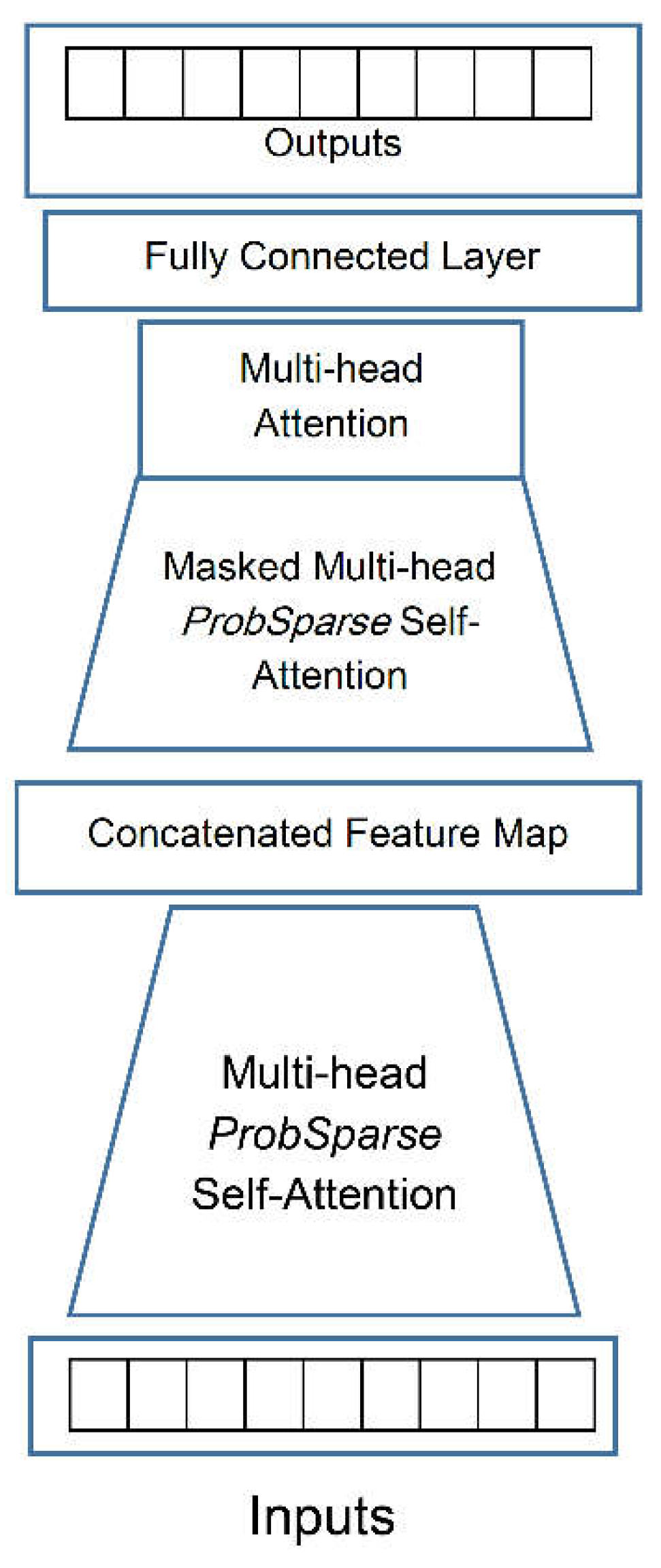
Given a time sequence at time t and the output corresponding sequence , the module encodes the input representations into a hidden state representation and decodes an output representations from . The extracted features of each series are added to the positional encoders, after the input series have been embedded and representative features have been created by the embedding module. We consider that we have t-th sequence input and p types of global time stamps and the feature dimension after input representation is . We first use a fixed position embedding to maintain the local context:
Where . A learnable stamp embedding utilizes every global time stamp with limited vocab size. Since the self-attention’s similarity computation can have access to global context, the computation consuming is affordable on long inputs. we project the scalar context into -dim vector with 1-D convolutional filters with kernel width equal to 3 and stride one to align the dimension. Thus, we have the feeding vector:
In this equation, is the factor balancing the magnitude between the scalar projection and local/global embedding that is set to 1 in this study, and .
Figure 2.
The encoder’s single stack in the Informer module.
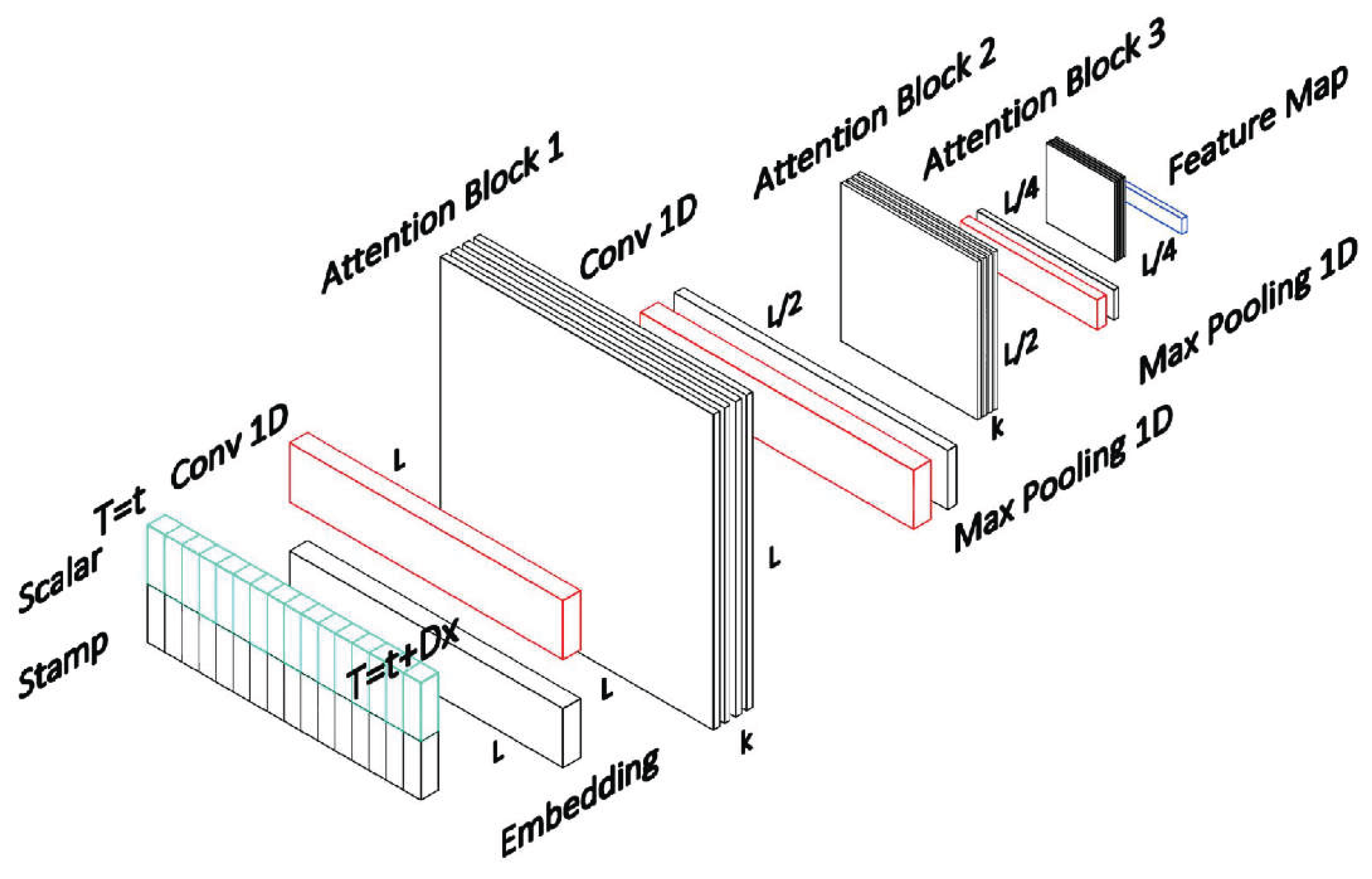
ProbSparse Self-attention. We apply the ProbSparse self-attention by allowing each key to only attend to the u dominant queries:
Where Q is a sparse matrix of the same size of q and it only contains the Top-u queries under the sparsity measurement .
Encoder. The encoder's purpose is to extract from the lengthy sequential inputs the reliable long-range dependency. As the input representation is done, the matrix will be the new shape of the t-th sequence input .
Self-attention Distilling. We use the distilling operation to privilege the superior ones with dominating features, because the natural consequence of the ProbSparse self-attention mechanism has redundant combinations of value . This also makes a focused self-attention feature map in the next layer. Observing the n-heads weights matrix of the Attention blocks in Fig. 2, it drastically reduces the input's time dimension. According to equation (6), the applied procedure forwards from j-th layer into (j + 1)-th layer.
In this formula, represents the attention block, is the activation function and is an 1D convolutional filter with kernel width of three. To reduces the whole memory usage, a max-pooling layer with stride 2 down samples into its half slice.
Decoder. We use a stack of two identical multi-head attention layers as the decoder, and to alleviate the speed plunge in long prediction, we apply the generative inference. The following vectors are given to the vanilla decoder as the input:
where and are is the start token and placeholder for the target sequence, respectively. The final layer is a dense layer that generates the results.
Generative Inference. Start token is efficiently applied in NLP’s “dynamic decoding” (Devlin et al. 2018), and we extend it into a generative way. We sample a long sequence in the input sequence, so contains target sequence’s time stamp, that is the context at the target. Instead of the cumbersome “dynamic decoding” in the vanilla encoder-decoder blocks, the decoder used in this study forecasts outputs by a forward procedure. We chose the MSE loss function across the entire Informer module.
Evaluation metrics. To evaluate the predictive capability of the proposed model for forecasting the ENSO, we computed the temporal anomaly correlation coefficient (ACC), which is defined as follows:
Here, is the predicted version of . denotes the difference between and the climatology, that is, the long-term mean of weather states that are estimated on the training data. Here, m and l are the calendar month (from 1 to 12) and the forecast lead months (1-36), respectively. The label y denotes the forecast target year. Finally, s and e denote the earliest (that is, 2001) and the latest year (that is, 2020) of the validation, respectively.
For deeper insight, we evaluated the method using Root Mean Square Error (RMSE) as follows:
Hyperparameters. The hyperparameters used in this study for the TSI module are as follows: number of encoder layers = 3, number of decoder layers = 2, embedding dimension = 512, number of attention heads = 8, dropout rate = 0.1, batch size = 32, and learning rate = 0.0001 with the Adam optimizer. These values were determined through systematic optimization using the ROA method (Talaat and Gamel 2022).
2.2. Implementation of Code and Cloud Super Computing
Python and TensorFlow (Abadi et al. 2016) were used to implement the proposed model. Part of the coding, debugging, and experimental execution was carried out in a cloud-based computational environment using Google Colaboratory, which provides a serverless Jupyter notebook interface with access to GPU/TPU acceleration for machine-learning workflows (Bisong 2019). The use of a streamlined time-series-only architecture substantially reduced the computational requirements compared with the earlier MEF framework. During model development, cloud resources were used for training and hyperparameter testing, while the final trained model could perform inference on a standard CPU within seconds. This makes the proposed framework suitable for reproducible research and future operational deployment without requiring a dedicated high-performance computing cluster.
2.3. Data Augmentation with CMIP5 and CMIP6
An innovative aspect of the new framework includes the systematic incorporation of historical simulations from the coupled model intercomparison project (CMIP5 & CMIP6). Previous studies examining ENSO using deep learning have either depended on a combination of CMIP5-only, as in Ham et al. (2019), or limited observational data when incorporating multiple model generations into prediction algorithms. The inclusion of CMIP5/CMIP6 brings three primary benefits:
First, the newer CMIP6 contains the most up-to-date historical simulations with improved physical parameterizations and an increase in spatial resolution compared with CMIP5. Secondly, the combined ensembles of CMIP5/CMIP6 will include a larger spread of variability for the ENSO phenomenon, resulting in a larger representation of rare extreme events than possible with only CMIP5. Third, training on multiple model generations will decrease the risk of overfitting the data, thus improving generalization of the model to observational data.
Compared to the earlier MEF framework, the current framework does not use the 3DCNN module; the entire training of the model is conducted with the TSI module only, using one-dimensional time series as input (primarily the monthly Niño 3.4 index, with other potential auxiliary indices such as IOD or PMM possibly augmenting the time series). The CMIP5 and CMIP6 data repositories are displayed in Table 1.
2.4. Input and Output Data
The input to the TSI module is the Niño 3.4 Index. This is the average sea surface temperature anomaly for the area between 120°W and 170°W and 5°S and 5°N. The Niño 3.4 Index is the way to describe El Niño and La Niña events. The TSI module uses this index to predict the Niño 3.4 Index for the 1 to 36 months.
The TSI module was trained using simulations from CMIP5 and CMIP6. These simulations are from 1850 to 2000. There are 21 CMIP5 models and 30 CMIP6 models. This gives us a lot of data to work with. The TSI module was fine-tuned using data from GODAS from 1980 to 2000. Then it was tested on GODAS data from 2001 to 2020. This way we know the TSI module is working well.
Our new model is different from the MEF framework. It only uses time-series data. It does not use maps of sea surface temperature anomalies. This makes it easier to store and process the data. We got 500 GB of raw data from CMIP5 and CMIP6. We used this data to get the Niño 3.4 Index for each model. We checked the data against data from GODAS and against processed data from Ham et al.
Table 1 shows where we got the data, from and where it is stored.
3. Results and Discussion
3.1. Overall Forecasting Skill
The proposed Informer-based prediction model was tested using GODAS observational data (2001-2020) and trained using merged CMIP5/CMIP6 historical data (1850-2000) and fine-tuned to GODAS (1980-2000) maintaining absolute separation between the two in terms of training and validating data.
The current Informer-based prediction model compared to previous MEF model uses only 1D time series data without complex spatial processing or ensemble voting. This architecture produces unprecedented long range skill.
The proposed Informer-based model demonstrates strong predictive skill at short and intermediate lead times, with ACC values decreasing gradually during the first 14 months. Beyond this period, the prediction skill remains relatively stable, fluctuating around 0.4–0.5 up to the 36-month lead time. Although the correlation decreases with increasing lead time, the model preserves useful predictive information over multi-year horizons. These results highlight the potential of deep learning approaches for extending ENSO prediction toward multi-year forecasting horizons.
On the other hand, The CNN benchmark shows a faster degradation of predictive skill compared with the proposed model. According to the available CNN results, the correlation decreases considerably after approximately 18 months and remains lower than the proposed framework at longer lead times. Similarly, the SINTEX-F dynamic model (Doi et al. 2019) degraded to less than 0.4 one month beyond the 18 month prediction period.
3.2. Seasonal Dependence and the Spring Predictability Barrier
The spring predictability barrier remains evident in the proposed model, although its effect is reduced compared with conventional dynamical and deep-learning approaches. At a 24-month lead time, the proposed model maintains ACC values above 0.45 for March–April–May targets. A direct comparison with the CNN benchmark is not reported at this lead time because corresponding CNN values were unavailable.
The decrease in the spring predictability barrier produced by the Informer is due to its use of a ProbSparse self-attention mechanism that allows it to choose the most informative time steps from the entire input sequence and, therefore, avoid the degradation of the signal relative to noise that has typically impacted the prediction of the ENSO during the boreal springtime.
3.3. Comparison with Benchmark Models
To evaluate the proposed model against an established deep-learning benchmark, its ACC values were compared with those of the CNN model developed by Ham et al. (2019) at selected forecast lead times (Table 2). The two models show similar skill at short lead times, but their performance diverges as the forecast horizon increases. The proposed model retains substantially higher ACC values at 12 and 18 months, indicating greater robustness at extended lead times. CNN results beyond 18 months were not available and were therefore neither plotted nor extrapolated.
The improved long-lead performance is consistent with the temporal focus of the Informer architecture. ProbSparse self-attention enables the model to identify informative dependencies across long input sequences, whereas the CNN benchmark relies primarily on spatial features. This distinction may explain the larger performance gap observed at longer lead times.
Figure 3 presents the values reported in Table 2 graphically. At lead times of 1 and 6 months, the differences between the two models are small, at 0.01 and 0.03, respectively. The gap increases to 0.08 at 12 months and 0.29 at 18 months. At the 18-month lead time, the proposed model achieves an ACC of 0.46, compared with 0.17 for the CNN benchmark. At 24 and 30 months, only the proposed model is shown because corresponding CNN results were unavailable.
3.4. Ablation Analysis: The Role of CMIP6 Data
An ablation experiment was performed where the Informer architecture was applied to train on only the CMIP5 data for performance comparison against the CMIP6 results. Other hyperparameters, training methods, and validation periods remained the same.
The model utilizing CMIP5 alone obtains ACC measurements of over 0.5 only for a period of 28 months. After that period, the ACC measurement declines further to a reading of 0.45 at 36 months. However, ACC measurement obtained from the full model of CMIP5 + CMIP6 maintains higher ACC values across long lead times, with the largest improvements observed during the 24–30 month prediction range.
When CMIP6 is added to the model, all lead times demonstrate higher performance than would have been shown with only CMIP5. Specifically, there are about 0.09 more ACC points of gain for lead time periods occurring between 24 and 30 months than what would have been shown based on CMIP5 only. This is most impressive given the fact that the lead time periods between 24 and 30 months are caused by factors that have been associated with major declines in skill from more traditional methodologies (which include both dynamical systems and previously implemented deep-learning based procedures).
These findings confirm three major points. First, adding CMIP6 to the dataset provides a strong advantage in terms of long-lead forecast skill through the combined training of the two datasets than only training with CMIP5. Second, the advantage of using CMIP6 data becomes more pronounced as lead time increases, supporting the hypothesis that the additional variability regimes captured by the CMIP6 dataset provide strong information for anticipating multi-year dynamics associated with the phenomena of ENSO. Third, improved performance during the period of validation that followed 2000 shows that having training from a wider ensemble of different climatic forecast model types provides better generalization ability for the new observational states of ENSO due to increased variability in ENSO over recent times.
3.5. Computational Efficiency
The proposed Informer model requires approximately 8 GPU hours for training, compared with 72 GPU hours for the original MEF framework and 12 GPU hours for the CNN benchmark. Its inference time is approximately 0.5 s per forecast, and inference can be performed on a standard CPU. By contrast, the original MEF framework and the CNN benchmark require GPU acceleration and have inference times of approximately 15 s and 2 s per forecast, respectively. The proposed model also requires only about 2 GB of GPU memory, compared with 45 GB for MEF and 8 GB for the CNN benchmark.

Table 3.
Computational efficiency comparison.
| Metric | Proposed Model | MEF (original) | CNN (Ham et al. 2019) |
|---|---|---|---|
| Training time (GPU hours) | 8 | 72 | 12 |
| Inference time (seconds per forecast) | 0.5 | 15 | 2 |
| GPU memory (GB) | 2 | 45 | 8 |
| CPU inference possible? | Yes | No | No |
4. Conclusion
We utilized the Multimodal ENSO Forecasting (MEF) approach to analyze previous findings and determine the driving factors of the forecast's long-range skill (beyond 18 months), using an ablation analysis method to conclude that the Informer time-series branch provided the majority of the long-range skill, with little contribution from the higher-dimensional spatial processing branch. With this new understanding, we re-evaluated the need for spatial complexity in the long-term forecast of ENSO events.
Based on that conclusion, we developed a new, simplified and improved Informer-only based predictive system that relies solely on inputting unidimensional climate signals. The combination of enhanced input representations, systematic hyperparameter optimization and expansion of the training set to include historical simulations (CMIP5 and CMIP6) has enabled the new model to produce unprecedented predictive ability.
The key findings of this study are as follows:
First, the proposed model maintained useful predictive skill at lead times of up to 36 months. Although ACC declined as the forecast horizon increased, it remained approximately within the 0.4–0.5 range at extended lead times and exceeded the benchmark models where directly comparable results were available. To our knowledge, this represents one of the longest lead times reported for deep-learning-based ENSO forecasting.
The results support this conclusion in that a larger dataset trained on different generations of climate models helps the model generalise better to the time period after 2000 when the variability of ENSO behaviour has increased.
Secondly, using only the Informer architecture requires very little compute; it takes about 8 hours of training time on one GPU, and inference can be completed in a few seconds on a regular CPU. In comparison, our original MEF framework used 72 GPU hours and needed 45 GB of memory, and other image-based deep learning models require more resources than this.
Thirdly, the lower spring predictability barrier in our model, which maintains correlations greater than 0.45 for MAM targets even at 24 month lead times, demonstrates that the ProbSparse attention mechanism is effective at capturing seasonal signatures that conventional models cannot retain.
In the future, the way forward will involve two main areas of focus: The integration of additional climate indices (e.g., IOD, PMM) into the model as auxiliary input signals, and extending the operational forecasting option based on transformer architecture beyond 36 months lead.
In general, the Informer Framework has established a new baseline for forecasting operational-long-lead ENSO's (El Niño-Southern Oscillation) using the best blend of accuracy, efficiency, and demonstrated skill to create a scalable and repeatable approach to time-series based climate prediction for those up to 36 months lead. Together this will demonstrate the potential of time-series learning architectures designed with climate-model informed training will significantly advance the development of long-lead climate predictions.
Author Contributions
All authors contributed to the study conception and design. Data collection and python coding were performed by Mohammad Naisipour and Iraj Saeedpanah. Analyses were performed by Mohammad Naisipour and Iraj Saeedpanah, with the supervision of Iraj Saeedpanah and Arash Adib. The first draft of the manuscript was written by Mohammad Naisipour and Iraj Saeedpanah. All authors commented on previous versions of the manuscript. All authors read and approved the final manuscript.
Funding
This work received no funding.
Data Availability Statement
The CMIP5 and CMIP6 historical simulations used to derive the Niño 3.4 time series are available through the Earth System Grid Federation repositories. GODAS observational data used for model calibration and validation are publicly available through the NOAA Physical Sciences Laboratory.
Conflicts of Interest
The authors have no relevant financial or non-financial interests to disclose.
Code Availability
The reproducible code and trained model configuration will be made available through a Google Colab notebook upon publication.
Additional Information
Correspondence and requests for materials should be addressed to Saghar Ganji.
Consent to Participate and Consent to Publish
The authors declared that they approved submitting the final manuscript.
References
- Abadi M, Agarwal A, Barham P, et al. (2016) TensorFlow: Large-Scale Machine Learning on Heterogeneous Distributed Systems. Distributed Parallel and Cluster Computing. arXiv:1603.04467. [CrossRef]
- Afshar MH, Naisipour M, Amani J (2011) Node moving adaptive refinement strategy for planar elasticity problems using discrete least squares meshless method. Finite Elements in Analysis and Design 47(12):1315-1325. [CrossRef]
- Anderson BT, Perez RC (2015) ENSO and non-ENSO induced charging and discharging of the equatorial Pacific. Climate Dynamics 45:2309–2327. [CrossRef]
- Babamiri O, Dinpashoh Y (2024) Uncertainty Analysis of River Water Quality Based on Stochastic Optimization of Waste Load Allocation Using the Generalized Likelihood Uncertainty Estimation Method. Water Resour Manage 38:967–989. [CrossRef]
- Bell G, Halpert DM, l’Heureux M (2015) ENSO and the Tropical Pacific. In State of the Climate 2015 Chapter 4: The Tropics. Diamond HJ, Schreck CJ Eds.
- Beucler T, Gentine P, Yuval J, et. al (2024) Climate-invariant machine learning. Science Advances 10 6. [CrossRef]
- Blöschl G, Hall J, Viglione A, et al. (2019) Changing climate both increases and decreases European river floods. Nature 573:108–111. [CrossRef]
- Cai W, Borlace S, Lengaigne M, et al. (2014) Increasing frequency of extreme El Niño events due to greenhouse warming. Nature Clim Change 4:111–116. [CrossRef]
- Cai W, McPhaden MJ, Grimm AM, et al. (2020) Climate impacts of the El Niño–Southern Oscillation on South America. Nat Rev Earth Environ 1:215–231. [CrossRef]
- Castangia M, Grajales L, Aliberti A, Rossi C (2023) Transformer neural networks for interpretable flood forecasting. Environmental Modelling & Software 160:105581. [CrossRef]
- Chang P, Zhang L, Saravanan R, et al. (2007) Pacific meridional mode and El Niño—Southern Oscillation. Geophys. Res Lett 34:L16608. [CrossRef]
- Chen H, Teegavarapu, RSV, Xu YP (2021) Oceanic-Atmospheric Variability Influences on Baseflows in the Continental United States. Water Resour Manage 35:3005–3022. [CrossRef]
- Chen HC, Tseng, YH, Hu, ZZ, et al. (2020) Enhancing the ENSO Predictability beyond the Spring Barrier. Sci Rep 10:984. [CrossRef]
- Chu H, Wei J, Jiang Y (2021) Middle- and Long-Term Streamflow Forecasting and Uncertainty Analysis Using Lasso-DBN-Bootstrap Model. Water Resour Manage 35:2617–2632. [CrossRef]
- Devlin J, Chang MW, Lee K, Toutanova K (2018) Bert: Pre-training of deep bidirectional transformers for language understanding. arXiv:1810.04805. [CrossRef]
- Dixit S, Jayakumar KV (2022) A Non-stationary and Probabilistic Approach for Drought Characterization Using Trivariate and Pairwise Copula Construction (PCC) Model. Water Resour Manage 36:1217–1236. [CrossRef]
- Doi T, Behera SK, Yamagata T (2019) Merits of a 108-Member Ensemble System in ENSO and IOD Predictions. J Climate 32:957–972. [CrossRef]
- Erdmann M, Glombitza J, Quast T (2019) Precise Simulation of Electromagnetic Calorimeter Showers Using a Wasserstein Generative Adversarial Network. Computing and Software for Big Science. 3:4. arXiv:1807.01954. [CrossRef]
- Fijani E, Khosravi K (2023) Hybrid Iterative and Tree-Based Machine Learning Algorithms for Lake Water Level Forecasting. Water Resour Manage 37:5431–5457. [CrossRef]
- Gao D, Chen AS, Memon FA (2024) A Systematic Review of Methods for Investigating Climate Change Impacts on Water-Energy-Food Nexus. Water Resour Manage 38:1–43. [CrossRef]
- Gao C, Zhang RH (2017) The roles of atmospheric wind and entrained water temperature (Te) in the second-year cooling of the 2010–12 La Niña event. Clim Dyn 48:597–617. [CrossRef]
- Giudicianni C, Di Cicco I, Di Nardo A, et al. (2024) Variance-based Global Sensitivity Analysis of Surface Runoff Parameters for Hydrological Modeling of a Real Peri-urban Ungauged Basin. Water Resour Manage 38:3007–3022. [CrossRef]
- Glorot X, Bengio Y (2010) Understanding the difficulty of training deep feedforward neural networks. Proceedings of the thirteenth international conference on artificial intelligence and statistics 249–56.
- Goodfellow I, Bengio Y, Courville A (2016) Deep Learning. MIT PRESS.
- Guan C. McPhaden MJ (2016) Ocean processes affecting the twenty- first-century shift in ENSO SST variability. J Clim 29:6861–6879. [CrossRef]
- Ham Y, Kim J, Luo J (2019) Deep learning for multi-year ENSO forecasts. Nature 573:568–572. [CrossRef]
- Ham YG, Kim JH. Kim ES, On KW (2021) Unified deep learning model for El Niño/Southern Oscillation forecasts by incorporating seasonality in climate data. Science Bulletin 66(13):1358-1366. [CrossRef]
- Ho J, Ermon S (2016) Generative Adversarial Imitation Learning. Advances in Neural Information Processing Systems. 29:4565–4573. arXiv:1606.03476. [CrossRef]
- Hunter JD (2007) Matplotlib: a 2D graphics environment. Comput Sci Eng 9:90–95.
- Isola P, Zhu J, Zhou T, Efros A (2017) Image-to-Image Translation with Conditional Adversarial Nets. Computer Vision and Pattern Recognition. [CrossRef]
- Izumo T, Vialard J, Lengaigne M, et al. (2010) Influence of the state of the Indian Ocean Dipole on the following year’s El Niño. Nature Geosci 3:168–172. [CrossRef]
- Jonnalagadda J, Hashemi M (2023) Long Lead ENSO Forecast Using an Adaptive Graph Convolutional Recurrent Neural Network. Eng Proc 39:5. [CrossRef]
- Karpathy A, Fei-Fei L (2015) Deep visual-semantic alignments for generating image descriptions. Proceedings of the IEEE Conference on Computer Vision and Pattern Recognition 3128-3137. 10.1109/CVPR.2015.7298932.
- Khan M, Kazmi SAA, Qureshi SR, et al. (2024) Repeatability of instantaneous position in rotational motion of a submerged Savonius turbine driven by water surface waves using image processing: an experimental investigation. J Ocean Eng Mar Energy 10:859–877. [CrossRef]
- Kilinc HC, Apak S, Ozkan F, et al. (2024) Multimodal Fusion of Optimized GRU–LSTM with Self-Attention Layer for Hydrological Time Series Forecasting. Water Resour Manage 38:6045–6062. [CrossRef]
- Kirtman B, Power SB (2013) The Physical Science Basis. Contribution of Working Group I to the Fifth Assessment Report of the Intergovernmental Panel on Climate Change (eds Stocker TF, Qin D, Plattner GK, et al.) Ch 11 Cambridge Univ Press.
- Kochkov D, Yuval J, Langmore I, et al (2024) Neural general circulation models for weather and climate. Nature 632:1060–1066. [CrossRef]
- Koldasbayeva D, Tregubova P, Gasanov M, et al. (2024) Challenges in data-driven geospatial modeling for environmental research and practice. Nat Commun 15:10700. [CrossRef]
- Kumshe UMM, Abdulhamid ZM, Mala BA, et al. (2024) Improving Short-term Daily Streamflow Forecasting Using an Autoencoder Based CNN-LSTM Model. Water Resour Manage 38:5973–5989. [CrossRef]
- Labibzadeh M, Modaresi R, Naisipour M (2015) Efficiency test of the discrete least squares meshless method in solving heat conduction problems using error estimation. Sharif Journal of Civil Engineering 31.2(3.2):31-40.
- L'Heureux ML, Levine AF, Newman M, Ganter C, Luo JJ, Tippett MK, et al. (2020). “ENSO prediction,” in El Niño Southern Oscillation in a Changing Climate. John Wiley & Sons 227–246. [CrossRef]
- Li H, Qian L, Yang J, et al. (2023) Parameter Estimation for Univariate Hydrological Distribution Using Improved Bootstrap with Small Samples. Water Resour Manage 37:1055–1082. [CrossRef]
- Ling F, Luo JJ, Li Y, et al. (2022) Multi-task machine learning improves multi-seasonal prediction of the Indian Ocean Dipole. Nat Commun 13:7681. [CrossRef]
- Luc P, Couprie C, Chintala S, Verbeek J (2016) Semantic Segmentation using Adversarial Networks. NIPS Workshop on Adversarial Training Dec Barcelona Spain. arXiv:1611.08408. [CrossRef]
- Luo J, Masson S, Behera SK, Yamagata T (2008) Extended ENSO predictions using a fully coupled ocean–atmosphere model. J Clim 21:84–93. [CrossRef]
- McPhaden MJ, Zebiak SE, Glantz MH (2006) ENSO as an integrating concept in Earth science. Science 314:1740–1745. https://www.science.org/doi/10.1126/science.1132588.
- Mekonnen A, Renwick JA, Sanchez-Lugo A (2015) Eds. Chapter 7: Regional Climates. In State of the Climate Blunden J and D. Arndt Eds.
- Mohamed S, Lakshminarayanan B (2016) Learning in Implicit Generative Models. arXiv:1610.03483. [CrossRef]
- Montgomery DC, Runger GC (2014) Applied Statistics and Probability for Engineers (6th ed.). Wiley 241.
- Mooers G, Pritchard M, Beucler T, Srivastava T (2024) Comparing storm resolving models and climates via unsupervised machine learning. Scientific Reports 13:22365. [CrossRef]
- Muhammad AU, Abba SI (2023) Transfer learning for streamflow forecasting using unguaged MOPEX basins data set. Earth Sci Inform 16:1241–1264. [CrossRef]
- Muhammad AU, Djigal H, Muazu T, et al. (2023) An autoencoder-based stacked LSTM transfer learning model for EC forecasting. Earth Sci Inform 16:3369–3385. [CrossRef]
- Mustafa M, Brad D, Bhimji W, et al. (2019) CosmoGAN: creating high-fidelity weak lensing convergence maps using Generative Adversarial Networks. Computational Astrophysics and Cosmology. 6(1): 1. arXiv:1706.02390. ISSN 2197-7909. [CrossRef]
- Naisipour M, Saeedpanah I, Adib A (2024) Novel Deep Learning Method for Forecasting ENSO. Journal of Hydraulic Structures 11(3):14-25. [CrossRef]
- Nicolas C, Francisco M, Gabriel S, Nicolas U, Alexander K, Sergey Z (2020) End-to-end object detection with transformers. Proceedings of ECCV 213-229.
- Oquab M, Bottou L, Laptev I, Sivic J (2014) Learning and transferring mid-level image representations using convolutional neural networks. In Proc. IEEE Conference. [CrossRef]
- Paganini M, de Oliveira L, Nachman B (2017) Learning Particle Physics by Example: Location-Aware Generative Adversarial Networks for Physics Synthesis. Computing and Software for Big Science. 1:4. arXiv:1701.05927. [CrossRef]
- Park JH, Kug JS, Li T, Behera SK (2018) Predicting El Niño beyond 1-year lead: effect of the Western Hemisphere warm pool. Sci Rep 8:14957. [CrossRef]
- Park JH, Kug JS, Yang YM, et al. (2023) Distinct decadal modulation of Atlantic-Niño influence on ENSO. npj Clim Atmos Sci 6:105. [CrossRef]
- Park JH, Yang YM, Ham YG, et al. (2024) Significant winter Atlantic Niño effect on ENSO and its future projection. npj Clim Atmos Sci 7:238. [CrossRef]
- Planton YY, Guilyardi E, Wittenberg AT, et al. (2021) Evaluating climate models with the CLIVAR 2020 ENSO metrics package. Bulletin of the American Meteorological Society 102(2):E193-E217. [CrossRef]
- Raftery AE, Gneiting T, Kitsui K (2005) Using Bayesian model averaging to forecast the likelihood of certain weather events. Monthly Weather Review 133(5):1155-1174. [CrossRef]
- Razmi A, Mardani-Fard HA, Golian S, et al. (2022) Time-Varying Univariate and Bivariate Frequency Analysis of Nonstationary Extreme Sea Level for New York City. Environ Process 9 8. [CrossRef]
- Ricke K, Caldeira K (2014) Natural climate variability and future climate policy. Nature Clim Change 4:333–338. [CrossRef]
- Rives A, Meier J, Sercu T, Goyal S, et al. (2016) Biological structure and function emerge from scaling unsupervised learning to 250 million protein sequences. Proc Natl Acad Sci 118(15):10.1073 pnas.2016239118. [CrossRef]
- Salamani D, Golling GT, Stewart GA, et al. (2018) Deep generative models for fast shower simulation in ATLAS. IEEE 14th International Conference on e-Science 348-348. [CrossRef]
- Saliman T, Goodfellow I, Zaremba W, Cheung V, Radford A, Chen X (2016) Improved Techniques for Training GANs. arXiv:1606.03498. [CrossRef]
- Scaife AA (2010) Impact of ENSO on European Climate. ECMWF Seminar on Predictability in the European and Atlantic regions ECMWF conference Shinfield Park Reading 83-91.
- Schawinski K, Zhang C, Zhang H, et al. (2017) Generative Adversarial Networks recover features in astrophysical images of galaxies beyond the deconvolution limit. Monthly Notices of the Royal Astronomical Society: Letters. 467(1):L110–L114. [CrossRef]
- Schurch NJ, Schofield P, Gierliński M, et al (2016) How many biological replicates are needed in an RNA-seq experiment and which differential expression tool should you use? RNA Jun 22(6):839-51. [CrossRef]
- Schwaller P, Laino T, Gaudin T, Bolgar P, Hunter C, Bekas C, Lee A (2019) Molecular transformer: A model for uncertainty-calibrated chemical reaction prediction. ACS Central Sci 5(9):1572-1583. [CrossRef]
- Shepherd TG (2014) Atmospheric circulation as a source of uncertainty in climate change projections. Nat Geosci 7:703–708. [CrossRef]
- Singh U, Sharma PK (2022) Seasonal Uncertainty Estimation of Surface Nuclear Magnetic Resonance Water Content using Bootstrap Statistics. Water Resour Manage 36:2493–2508. [CrossRef]
- Spiliotis M, Tsakiris G (2017) Incorporating uncertainty in the design of water distribution systems. Ewra European Water 58:449–456.
- Talaat FM, Gamel SA, (2022) RL based hyper-parameters optimization algorithm (ROA) for convolutional neural network. J Ambient Intell Human Comput. [CrossRef]
- Tsakiris G, Spiliotis M (2016) Uncertainty in the Analysis of Water Conveyance Systems. Procedia Engineering 162:340-348. [CrossRef]
- Tsakiris G. Spiliotis M. (2017) Uncertainty in the analysis of urban water supply and distribution systems. J Hydroinformatics 19:823–837. [CrossRef]
- Vaswani A, Shazeer N, Parmar N, et al. (2017) Attention is all you need. Proceedings of NeurIPS 5998-6008. [CrossRef]
- Vatanchi SM, Maghrebi MF (2024) Calibration and Uncertainty Analysis for Isovel Contours-based Stage-discharge Rating Curve by Sequential Uncertainty Fitting (SUFI-2) Method. Water Resour Manage. [CrossRef]
- Vimont DJ, Wallace JM Battisti DS (2003) The seasonal footprinting mechanism in the Pacific: implications for ENSO. Journal of Climate 16:2668–2675. [CrossRef]
- Wang GG, Cheng H, Zhang Y, Yu H (2023) ENSO analysis and prediction using deep learning: A review. Neurocomputing 520:216-229. [CrossRef]
- Wang R, He J, Luo JJ, Chen L (2024) Atlantic Warming Enhances the Influence of Atlantic Niño on ENSO. Geophisical Research Letters 51(8):1-12. [CrossRef]
- Wang H, Hu S, Guan C, et al. (2024) The role of sea surface salinity in ENSO forecasting in the 21st century. npj Clim Atmos Sci 7:206. [CrossRef]
- Wang Z, Si Y, Chu H (2022) Daily Streamflow Prediction and Uncertainty Using a Long Short-Term Memory (LSTM) Network Coupled with Bootstrap. Water Resour Manage 36:4575–4590. [CrossRef]
- Xia B (2024) Enhancing 3D object detection through multi-modal fusion for cooperative perception. Alexandria Engineering Journal 104:46-55. [CrossRef]
- Ye F, Hu J, Huang T, You L, Weng B, Gao J (2022) Transformer for EI Niño-Southern Oscillation Prediction. IEEE Geoscience and Remote Sensing Letters 19:1-5. [CrossRef]
- Yoo JH, Kang IS (2005) Theoretical examination of a multi-model composite for seasonal prediction. Geophys Res Lett 32:L18707. [CrossRef]
- Zhao J, Luo H, Sang W, et al. (2023) Spatiotemporal semantic network for ENSO forecasting over long time horizon. Appl Intell 53:6464–6480. [CrossRef]
- Zhou H, Zhang S, Peng J, et al. (2021) Informer: Beyond Efficient Transformer for Long Sequence Time-Series Forecasting. AAAI-21. [CrossRef]
- Zhou L, Zhang RH (2022) A Hybrid Neural Network Model for ENSO Prediction in Combination with Principal Oscillation Pattern Analyses. Adv Atmos Sci 39:889–902. [CrossRef]
- Zhou L, Zhang RH (2023) A self-attention–based neural network for three-dimensional multivariate modeling and its skillful ENSO predictions. Sci Adv 9:eadf2827. [CrossRef]
- Jia L, Guo Y (2025) Increased Frequency of Central Pacific El Niño Events Since 2000 Caused by Frequent Anomalous Warm Zonal Advection. Atmosphere 16(6):654. [CrossRef]
- World Meteorological Organization (WMO) (2025) State of the Global Climate 2024. World Meteorological Organization, Geneva. https://wmo.int/publication-series/state-of-global-climate/state-of-global-climate-2024.
- World Meteorological Organization (WMO) (2026a) WMO: Prepare for El Niño. World Meteorological Organization, Geneva. https://wmo.int/news/media-centre/wmo-prepare-el-nino.
- World Meteorological Organization (WMO) (2026b) European State of the Climate 2025: Record heatwaves from the Mediterranean to the Arctic, while glaciers shrink and snow cover declines. World Meteorological Organization, Geneva. https://wmo.int/news/media-centre/european-state-of-climate-2025-record-heatwaves-from-mediterranean-arctic-while-glaciers-shrink-and.
- World Meteorological Organization (WMO) (2026c) Records fall as extreme heat grips Europe. World Meteorological Organization, Geneva. https://wmo.int/media/news/records-fall-extreme-heat-grips-europe.
- Bisong E (2019) Google Colaboratory. In: Building Machine Learning and Deep Learning Models on Google Cloud Platform. Apress, Berkeley, CA. [CrossRef]
- Chen Y, Jin Y, Liu Z, Shen X, Chen X, Lin X, Zhang R-H, Luo J-J, Zhang W, Duan W, Zheng F, McPhaden MJ (2025) Combined dynamical-deep learning ENSO forecasts. Nature Communications. [CrossRef]
- Mu B, Cui Y, Yuan S, Qin B (2024) Incorporating heat budget dynamics in a Transformer-based deep learning model for skillful ENSO prediction. npj Climate and Atmospheric Science 7:208. [CrossRef]
- Naisipour M, Saeedpanah I, Adib A (2025a) Multimodal Deep Learning for Two-Year ENSO Forecast. Water Resources Management 39:3745–3775. [CrossRef]
- Naisipour M, Saeedpanah I, Adib A (2026) Metrics matters: A deep assessment of deep learning CNN method for ENSO forecast. Atmospheric Research 330:108545. [CrossRef]
- Reuters (2026) At least 3,700 excess deaths reported during heatwave in France, Belgium and Netherlands. Reuters, 3 July 2026.
- World Meteorological Organization (WMO) (2026d) Record-breaking heat spreads through Europe. World Meteorological Organization, Geneva. https://wmo.int/media/news/record-breaking-heat-spreads-through-europe.
- Zhou L, Zhang R-H (2026) Tropical basin interactions reduce spring predictability barrier of ENSO in a deep learning model. Science Advances 12(21):eaeb0901. [CrossRef]
Figure 3.
Anomaly correlation coefficient (ACC) of the proposed Informer-based model and the CNN benchmark at selected forecast lead times. Values are taken from Table 2. Because CNN results were unavailable at 24 and 30 months, the CNN curve terminates at 18 months.
Figure 3.
Anomaly correlation coefficient (ACC) of the proposed Informer-based model and the CNN benchmark at selected forecast lead times. Values are taken from Table 2. Because CNN results were unavailable at 24 and 30 months, the CNN curve terminates at 18 months.
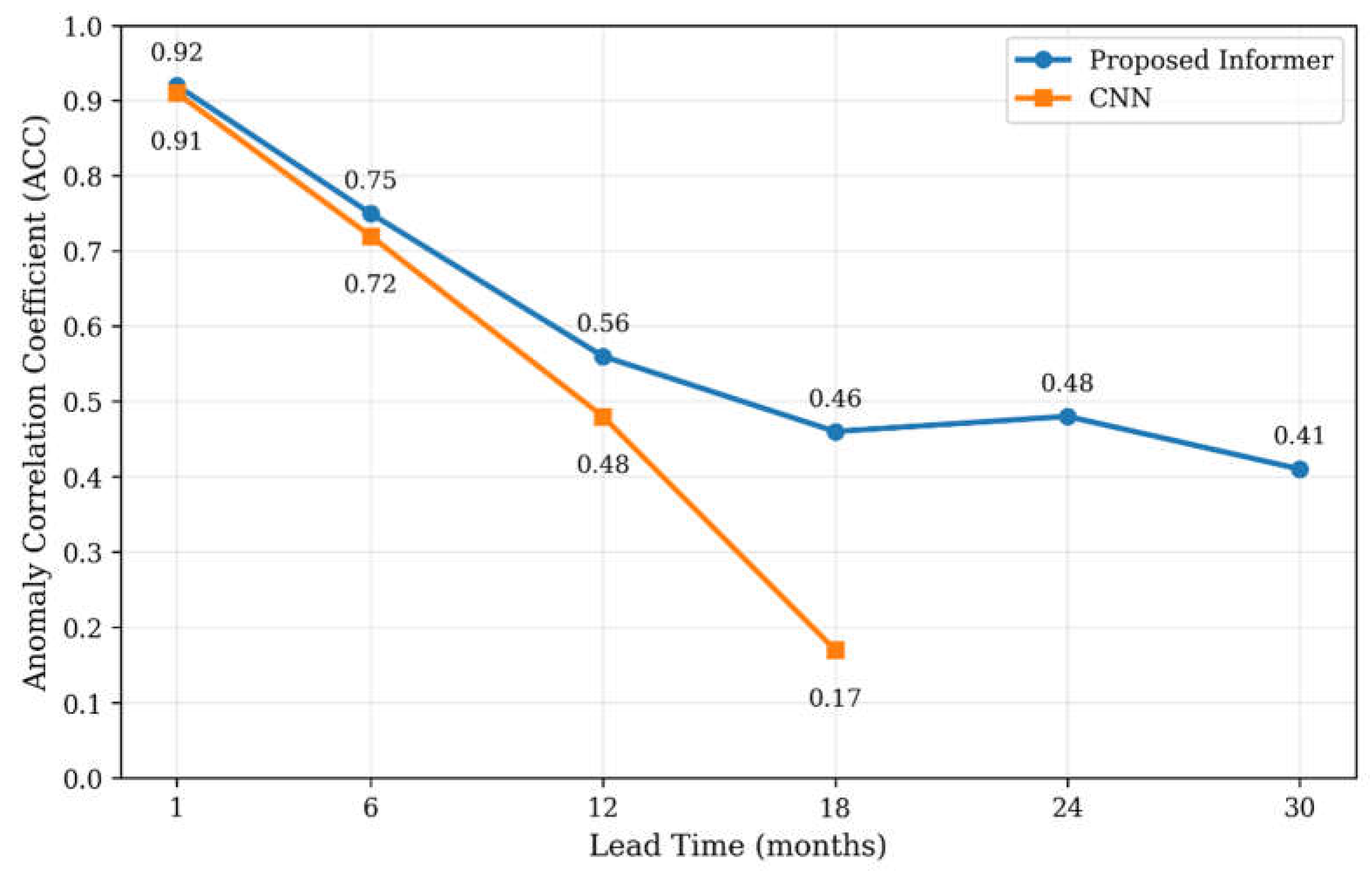
Table 1.
List of data and their repositories.
| Title | Application | Repository Address |
|---|---|---|
| CMIP5 | Training the TSI module | https://esgf-node.llnl.gov/projects/cmip5/ |
| CMIP6 | Augmented training data | https://esgf-node.llnl.gov/projects/cmip6/ |
| GODAS (Nino 3.4 Index) | Input of the TSI module and validation of the results |
https://www.esrl.noaa.gov/psd/data/gridded/data.godas.htm https://psl.noaa.gov/gcos_wgsp/Timeseries/Nino34/ |
Table 2.
Comparison of anomaly correlation coefficient (ACC) values for the proposed Informer-based model and the CNN benchmark at selected forecast lead times.
Table 2.
Comparison of anomaly correlation coefficient (ACC) values for the proposed Informer-based model and the CNN benchmark at selected forecast lead times.
| Lead Time (months) | Proposed Informer | CNN |
| 1 | 0.92 | 0.91 |
| 6 | 0.75 | 0.72 |
| 12 | 0.56 | 0.48 |
| 18 | 0.46 | 0.17 |
| 24 | 0.48 | — |
| 30 | 0.41 | — |
Disclaimer/Publisher’s Note: The statements, opinions and data contained in all publications are solely those of the individual author(s) and contributor(s) and not of MDPI and/or the editor(s). MDPI and/or the editor(s) disclaim responsibility for any injury to people or property resulting from any ideas, methods, instructions or products referred to in the content. |
© 2026 by the authors. Licensee MDPI, Basel, Switzerland. This article is an open access article distributed under the terms and conditions of the Creative Commons Attribution (CC BY) license.
Copyright: This open access article is published under a Creative Commons CC BY 4.0 license, which permit the free download, distribution, and reuse, provided that the author and preprint are cited in any reuse.