Preprint
Article

This version is not peer-reviewed.

Similarity Structure of Unsteady Incompressible Two-Fluid Plasma Boundary Layers

Submitted:

24 August 2026

Posted:

26 August 2026

You are already at the latest version

Abstract

We construct from first principles the complete similarity structure of unsteady incompressible two-fluid (Hall) plasma boundary layers with separate ion and electron temperatures, and analyse the resulting states in full. We first establish four exact degeneracies of the planar problem that constrain any admissible formulation: the Hall force cancels identically from the total momentum equation; the electron-pressure (Biermann) term vanishes identically from the induction equation at constant density; if the out-of-plane field \(B_z\) is set to zero the Hall term drops out of the in-plane flux equation altogether, so that a strictly planar "Hall boundary layer" is indistinguishable from resistive magnetohydrodynamics; and the \(B_z\) magnetic pressure cancels exactly from streamwise momentum. The minimal consistent description is therefore a four-field system in (\(\psi, B_Z, \mu_\perp, \mu_Z\)) coupled to two temperatures. Reducing this system under the two-parameter similarity map \(\eta=y/\delta(x)\), \(\tau=\nu t/\delta^{2}(x)\), we prove an exhaustive classification theorem: exact similarity of the full two-fluid problem requires \(\delta'(x)=0\), which admits precisely two nondegenerate families—a stagnation-type layer with \(U_e\propto x\), exactly self-similar to all orders in the Hall parameter \(\varepsilon_H=Md_i/\delta\), and a degenerate Rayleigh layer—while the Blasius-type growing layer is self-similar exactly through first order in \(\varepsilon_H\) and breaks similarity only at \(O(\varepsilon_H^{2})\). The obstruction is intrinsic: \(d_i\) is an absolute length while \(\delta\) grows, so Hall physics in a growing layer is a leading-edge phenomenon confined to \(x\lesssim x_H\) with \(x_H/d_i=\tfrac12M^{2}\mathrm{Re}_{d_i}\). We derive the reduced systems, their boundary conditions, and a set of von K\'arm\'an integral relations in full detail; obtain the asymptotic hierarchy in \(\varepsilon_H\); and identify the dispersive whistler scale \(d_i/\delta=\varepsilon_H/M\). Numerical solutions of the steady boundary-value problem and of the unsteady initial-value problem—the latter requiring implicit integration because the Hall coupling is a stiff fourth-order whistler operator—confirm every structural prediction, including an exact identity between the viscous and magnetic displacement thicknesses. A linear stability analysis shows the similarity states to be stable, with a leading eigenvalue that reproduces the measured relaxation rate to 0.6%, equals -1 exactly in the field-free limit for all \(P_m\) (a mode we identify analytically), vanishes linearly at the Alfvénic point as -1.36(1-\(M^{2}\)), and becomes complex near \(\varepsilon_H\simeq0.4\), so that relaxation turns oscillatory under the whistler coupling. We close by mapping the accessible regime onto laboratory and space plasmas using Braginskii transport, and by stating plainly where the collisional description fails.
Keywords: 
;  ;  ;  ;  ;  

1. Introduction

1.1. Background

Boundary layers are the archetype of singular-perturbation structure in fluid mechanics, and their similarity solutions—Blasius, Falkner–Skan, Hiemenz, Rayleigh–Stokes—remain the reference points against which more complicated flows are understood [1,2]. In electrically conducting fluids the same programme was carried out for single-fluid magnetohydrodynamics (MHD) in the late 1950s and 1960s. Greenspan and Carrier [3], Sears [4], Sears and Resler [5], and Gribben [6] established the structure of aligned-field MHD boundary layers, in which an ambient magnetic field parallel to the free stream is swept into the layer and the flow character changes qualitatively as the Alfvén number passes through unity. Stewartson’s analysis of the impulsively started plate [7] supplied the corresponding unsteady similarity framework, in which a single variable τ t / x interpolates between a diffusive Rayleigh layer and a convective Blasius layer. Similarity reductions of this two-parameter type continue to be developed for unsteady laminar layers [8].
Plasmas, however, are not single fluids. When the layer thickness approaches the ion inertial length d i = c / ω p i , ions and electrons decouple: the magnetic field remains frozen to the electron fluid while the ions slip across it. This is the Hall regime, and its signature in two dimensions is universal and unmistakable—an out-of-plane magnetic field with quadrupolar symmetry, generated by the in-plane electron current and mediated by dispersive whistler dynamics. The quadrupole was predicted by Sonnerup [9] and by Terasawa [10], established as the controlling ingredient of fast reconnection by Mandt, Denton and Drake [11], confirmed across the whole hierarchy of models in the GEM challenge [12], analysed asymptotically by Uzdensky and Kulsrud [13], and measured directly in the laboratory and in space [14,15,16]. If Hall physics is to be incorporated into boundary-layer similarity theory, the quadrupole must be the object that the theory produces.

1.2. What This Paper Establishes

This is a stronger constraint than it may appear, and it is the starting point of the present work. We show in Sec. 2 that a planar two-fluid model formulated with in-plane fields only is incapable of containing any Hall physics at all: the Hall term multiplies a triple product that vanishes identically. Three further exact degeneracies accompany it. Together these four lemmas eliminate every route by which Hall or electron-pressure effects might be thought to enter a constant-density planar layer, and they force the minimal consistent model to be a four-field system carrying B z and u z .
With the correct model in hand we ask what similarity structure it admits. The answer, Theorem 4.2 of Sec. 4, is sharper than in the single-fluid case. The magnetic and viscous groups can always be held constant by an appropriate choice of the external flow, but the Hall group ε H = M d i / δ contains the absolute length d i , which cannot be rescaled. Exact similarity therefore demands a layer of constant thickness. This selects the stagnation-type family U e = a x , δ = ν / a , for which we obtain a closed, exactly self-similar two-fluid system valid at arbitrary  ε H ; and it excludes the Blasius-type growing layer, for which similarity nevertheless survives exactly through O ( ε H ) and fails only at O ( ε H 2 ) . The physical content of the obstruction is a prediction: in a growing layer the Hall effect is a leading-edge phenomenon, active only within x x H where x H / d i = 1 2 M 2 Re d i .

1.3. Summary of Principal Results

For the reader’s convenience we list the results established below, with forward references.
1.
Four exact degeneracies (Lemmas 1–4, Sec. 2). The Hall force cancels from total momentum; the Biermann term cancels from induction at constant density; the Hall term cancels from the in-plane flux equation when B z 0 ; and the B z magnetic pressure cancels from streamwise momentum. The minimal consistent model is the four-field system (18)–(20).
2.
The Hall similarity parameter is ε H = M d i / δ [Equation (35)], with B z ε H B x e and u z ε H M 2 U e .
3.
Classification theorem (Theorem 4.2). Exact similarity of the two-fluid problem requires δ = 0 ; the admissible families are the stagnation-type layer (exact to all orders in ε H ), the degenerate Rayleigh layer, and the Blasius-type layer (exact through O ( ε H ) only).
4.
Leading-edge confinement: in a growing layer ε H x 1 / 2 and Hall physics is confined to x x H with x H / d i = 1 2 M 2 Re d i [Equation (61)].
5.
Divergence structure of the Class-A Hall subsystem, which collapses to the first-order pair (58), and the associated redundancy of the perfectly conducting wall condition (Sec. 5 C).
6.
Displacement identity β = α [Equation (72)], verified to six figures and shown in Sec. 11 to correspond to an exact eigenvalue σ = 1 .
7.
Three-tier asymptotic hierarchy in ε H (Sec. 8 A), verified numerically over a decade.
8.
Hall length in similarity units is ε H / M , linear in ε H [Equation (93)], from the whistler branch ω 2 = k 2 v A 2 ( 1 + k 2 d i 2 ) .
9.
Linear stability (Sec. 11): the similarity states are attractors; the leading eigenvalue reproduces the measured relaxation rate to 0.6 % , vanishes linearly at the Alfvénic point, and becomes complex above ε H 0.4 , so that relaxation turns oscillatory.
10.
Validity constraint ε H 2 = M 2 Re L ( d i / L ) 2 [Equation (111)], which shows that small ε H and large Re L are in tension in collisional plasmas.

1.4. Organisation and How to Read This Paper

The paper is written to be self-contained. All reductions are carried out explicitly; no step is left as “it can be shown”. Readers already familiar with MHD boundary layers may proceed directly to Sec. 4.
Section 2 derives the four-field model and proves the four degeneracies. Section 3 fixes the distinguished limit. Section 4 carries out the similarity reduction and proves the classification theorem. Section 5 is devoted entirely to boundary conditions, which in this problem are unusually delicate: two physically reasonable wall models give different conditions on B z , and for the Blasius-type layer one of them turns out to be redundant with the far-field decay. Section 6 derives von Kármán-type integral relations, which serve both as physical interpretation and as numerical checks. Section 7 treats the dual-temperature energy equations. Section 8 establishes the ε H hierarchy and the whistler scale. Section 9 describes the numerical methods, including why an implicit integrator is unavoidable. Section 10 presents the results, and Sec. 11 the linear stability analysis. Section 16 maps the theory onto real plasmas and states its limits. Section 17 concludes.
Six appendices contain the detailed algebra: the full reduction of every equation (Appendix A), the general non-similar momentum equation and its Rayleigh limit (Appendix B), the wall-model analysis (Appendix C), the O ( ε H 2 ) correction problem (Appendix D), the linearised stability operator (Appendix E), and numerical parameters (Appendix F).
Table 1. Principalsymbols.
Symbol Meaning
u , u e ion (mass) and electron velocity
ψ in-plane flux function, B = × ( ψ z ^ )
B z , u z out-of-plane field and velocity
n , ρ = m i n number and mass density (both constant)
λ = 1 / μ 0 n e Hall coefficient
η m = η r / μ 0 magnetic diffusivity
ν = μ / ρ kinematic (ion) viscosity
d i = c / ω p i ion inertial length
v A B x e / μ 0 ρ , Alfvén speed
ω c i v A / d i , ion cyclotron frequency
δ ( x ) boundary-layer thickness scale
η , τ y / δ and ν t / δ 2
D η η + 2 τ τ , Euler operator
f , g , h , w reduced ϕ , ψ , B z , u z
θ i , θ e reduced ion/electron temperatures
M = v A / U e Alfvén number
ε H = M d i / δ Hall similarity parameter
P m = ν / η m magnetic Prandtl number
Pr i , Pr e ion/electron Prandtl numbers
Γ = 1 / a τ Δ equipartition parameter
Λ = δ δ U e / ν growth group
β ^ = δ 2 U e / ν pressure-gradient group
α , β viscous / magnetic displacement
σ stability eigenvalue

2. Two-Fluid Model and Exact Planar Reduction

2.1. Species Equations and Closure

We begin from the two-fluid equations for a quasineutral plasma of singly charged ions ( Z = 1 ) of mass m i and electrons of mass m e , with common number density n enforced by quasineutrality. The species momentum equations are
m i n t u i + u i · u i = p i + e n E + u i × B
· π i + R i e , m e n t u e + u e · u e = p e e n E + u e × B
· π e R i e ,
where R i e is the friction force exerted on ions by electrons and π s are the viscous stresses. We adopt the standard boundary-layer closure: electron inertia is neglected ( m e 0 ), electron viscosity is neglected relative to ion viscosity (their ratio is O ( m e / m i ) ), the ion stress is taken isotropic with dynamic viscosity μ = ρ ν , and the friction is the resistive form R i e = e n η r J with η r the resistivity.
Two consequences follow immediately and are used throughout. Neglecting m e in Equation (2) gives the generalized Ohm’s law,
E + u e × B = η r J p e e n ,
and, using u e = u J / n e so that u e × B = u × B ( J × B ) / n e ,
E + u × B = η r J + 1 n e J × B p e
in which the second and third terms on the right are the Hall and electron-pressure contributions. The current is J = e n ( u i u e ) = μ 0 1 × B , so that
u e = u J n e , u u i .
We take the plasma incompressible with uniform density,
n = const , · u = 0 · u e = 0 ,
the last equality because · J = 0 identically. Throughout we write
λ 1 μ 0 n e , η m η r μ 0 , d i = c ω p i = 1 n e ρ μ 0 ,
so that
λ μ 0 ρ = d i , λ 2 μ 0 ρ = d i 2 , v A d i = ω c i = e B m i .
The reader may find it useful to note that λ is the only place the elementary charge enters, and that every Hall effect in what follows is proportional to it.

2.2. Four Exact Degeneracies

The following four lemmas are elementary but decisive: they remove, exactly and without approximation, the terms through which Hall and electron-pressure physics are most often supposed to enter a planar layer. We prove each in full, because the errors they exclude are easy to make and hard to detect once the equations have been nondimensionalized.

2.2.1. Lemma 1: No Hall Force in Total Momentum

Lemma 1. The Hall term does not appear in the total (single-fluid) momentum equation.
Proof. 
Add Eqs. (1) and (2). The friction forces cancel by Newton’s third law. The electromagnetic forces sum to
e n E + u i × B e n E + u e × B = e n u i u e × B = J × B .
With m e 0 and p = p i + p e this gives
ρ t u + u · u = p + J × B + μ 2 u .
No term proportional to λ survives. □
The physical content is that the Hall force is internal to the electron–ion system: it transfers momentum between species but not to the mixture. Adding a separate Hall force to Equation (10) double counts J × B . The Hall effect enters the dynamics only through Equation (4), that is, only through induction.

2.2.2. Lemma 2: Biermann Degeneracy at Constant Density

Lemma 2. For n = const the electron-pressure term makes no contribution to the induction equation: × ( n e ) 1 p e 0 .
Proof. 
With n uniform the bracket equals ( p e / n e ) , a pure gradient, whose curl vanishes identically. □
More generally × [ ( n e ) 1 p e ] = ( n e ) 2 e n × p e , so a thermoelectric (Biermann battery) contribution requires n × p e 0 , that is, misaligned density and pressure gradients. The constant-density model excludes this by construction. In component form the degeneracy reads
× p e n e z = 1 n e x y p e y x p e = 0 ,
and we emphasize that the two terms in Equation (11) must be retained or discarded together. Keeping x y p e while dropping its partner produces a spurious source proportional to x y T e .

2.2.3. Lemma 3: Planar Hall Degeneracy

Lemma 3. Let B = × ( ψ z ^ ) be strictly planar, i.e., B z 0 . Then the Hall term drops out of the flux-transport equation identically, and the model reduces to resistive MHD.
Proof. 
With B = ( y ψ , x ψ , 0 ) and z 0 ,
μ 0 J = × B = 0 , 0 , 2 ψ ,
so J is purely out of plane. The z-component of Ohm’s law (4) contains the Hall contribution ( J × B ) z / n e = ( J x B y J y B x ) / n e , which vanishes because J x = J y = 0 . Equivalently, in flux form the field is advected by u e ,
t ψ + u e · ψ = η m 2 ψ ,
and u e · ψ = u · ψ ( n e ) 1 J · ψ = u · ψ since J = 0 . □
Restoring B z changes this completely. Now J = μ 0 1 ( y B z , x B z , 0 ) and
J · ψ = 1 μ 0 y B z x ψ x B z y ψ = 1 μ 0 y ψ x B z x ψ y B z = 1 μ 0 B · B z ,
where we used B = ( y ψ , x ψ ) . Hence
u e · ψ = u · ψ + λ B · B z .
Lemma 3 is the two-dimensional statement of a fact familiar from reconnection theory [9,11,13]: in two dimensions the Hall effect is the out-of-plane field. A model that discards B z has discarded the Hall effect, however many factors of λ its equations appear to contain.

2.2.4. Lemma 4: Cancellation of B z from Streamwise Momentum

This lemma is proved in Sec. 2.5 after the boundary-layer form is introduced, since it involves the pressure elimination.

2.3. The Four-Field Model

We now assemble the closed system. Uncurling Equation (13) with the Hall term (15) restored gives the flux equation; the z-component of Faraday’s law gives the B z equation; and the z-component of Equation (10) gives the u z equation.
For the B z equation it is cleanest to use t B = × ( u e × B ) + η m 2 B together with the identity × ( a × b ) = a ( · b ) b ( · a ) + ( b · ) a ( a · ) b . With · u e = · B = 0 the z-component is
t B z = B · u e z u e · B z + η m 2 B z .
Two simplifications occur. First,
J · B z = 1 μ 0 y B z x B z x B z y B z = 0 ,
so u e · B z = u · B z : the Hall drift does not advect B z . Second, u e z = u z J z / n e = u z + λ 2 ψ , so the stretching term splits into a fluid part and a Hall part. The result is the four-field system
t ψ + u · ψ + λ B · B z = η m 2 ψ + E 0 ( t ) , t B z + u · B z = B · u z
+ λ B · ( 2 ψ ) + η m 2 B z ,
ρ t u z + u · u z = 1 μ 0 B · B z + μ 2 u z ,
together with Equation (10) for u . Here E 0 ( t ) is a spatially uniform applied electric field (a loop voltage). Its origin is the residual gauge freedom: writing B = × A with A z = ψ and E = Φ t A , a potential Φ = E 0 ( t ) z + φ ( x , y , t ) is admissible in a z-independent problem and contributes a uniform E z = E 0 . Equivalently ψ ψ + c ( t ) shifts E 0 by c ( t ) .
Equations (18)–(20) are the standard incompressible Hall-MHD four-field system [17,18]; we have rederived them to make explicit which terms survive and which do not.

2.4. Energy Budget and the Dissipationless Hall Term

It is worth verifying at the outset that the Hall term transports but does not dissipate energy, since this fixes the structure of the thermal problem in Sec. 7. The magnetic energy evolves as
t B 2 2 μ 0 = J · E ( Poynting ) ,
and from Equation (4)
J · E = J · ( u × B ) + η r | J | 2 + J · ( J × B ) n e J · p e n e .
The third term vanishes identically because J · ( J × B ) = 0 : the Hall electric field is perpendicular to the current and does no work. The fourth term integrates to a surface contribution for constant n since · J = 0 . Hence the only volumetric sink is η r | J | 2 . Any formulation exhibiting an explicit “Hall heating” term has mis-assigned the electron work.

2.5. Boundary-Layer Form

Let x be streamwise, y wall-normal, and introduce the boundary-layer parameter ϵ = δ / L 1 with u x U , B x B , y δ 1 , x L 1 . Solenoidality gives u y ϵ U and B y ϵ B , and 2 y 2 at leading order.
Writing the Lorentz force explicitly,
( J × B ) x = J y B z J z B y = B z x B z μ 0 + B y y B x μ 0 ,
( J × B ) y = J z B x J x B z = y B x 2 + B z 2 2 μ 0 ,
where we used μ 0 J z = x B y y B x y B x , μ 0 J x = y B z and μ 0 J y = x B z . The y-momentum balance therefore gives, to leading order,
Π p + B x 2 + B z 2 2 μ 0 = Π ( x , t ) .
Lemma 4. The out-of-plane field contributes nothing to the streamwise momentum equation.
Proof. 
Eliminate p using Equation (25):
x p = x Π + B x x B x + B z x B z μ 0 .
Adding Equation (23), the terms ± B z x B z / μ 0 cancel identically, leaving
x p + ( J × B ) x = x Π + B x x B x + B y y B x μ 0 .
The same cancellation occurs in the free stream, where J 0 and ρ D t U e = x Π + μ 0 1 B x e x B x e , so the elimination of Π is unaffected by B z . □
Hence
ρ t u x + u x x u x + u y y u x = ρ t U e + U e x U e + 1 μ 0 B x x B x + B y y B x B x e x B x e + μ y 2 u x .
Lemma 4 is the mechanical counterpart of Lemma 1: the Hall effect influences streamwise momentum only indirectly, by modifying B x and B y through Equation (18). The remaining boundary-layer equations are
t ψ + u x x ψ + u y y ψ + λ B x x B z + B y y B z
= η m y 2 ψ + E 0 ( t ) , t B z + u x x B z + u y y B z = B x x u z + B y y u z + η m y 2 B z
+ λ B x x y 2 ψ + B y y 3 ψ , ρ t u z + u x x u z + u y y u z
= 1 μ 0 B x x B z + B y y B z + μ y 2 u z .

2.6. Free-Stream Compatibility

Outside the layer the plasma is ideal and the flux is frozen in. Evaluating Equation (29) as y with u x U e , B x B x e , B z 0 and ψ B x e y + ψ 0 ( x , t ) gives, at O ( y ) ,
t B x e + U e x B x e B x e x U e = 0 .
This is nothing but the statement that the external field line through a fluid element is stretched at the rate at which the element is stretched. For a steady external state it integrates to
B x e ( x ) U e ( x ) M 2 B x e 2 μ 0 ρ U e 2 = const .
Constancy of the Alfvén number is thus not an extra assumption but a consequence of ideal external induction. This will matter in Sec. 4: it removes one apparent degree of freedom and makes the Hall constraint binding.

3. Boundary-Layer Ordering and the Hall Parameter

3.1. The Distinguished Limit

We now fix the orders of B z and u z . Consider Equation (30). The Hall source is
λ B x x y 2 ψ + B y y 3 ψ λ B 2 δ L + ϵ B 2 δ 2 λ ϵ B 2 δ 2 ,
both contributions being of the same order because ϵ = δ / L . The advective terms are U B z / L = ϵ U B z / δ . Balancing,
B z λ B 2 U δ = ε H B , ε H λ B x e U e δ = M d i δ
where M = v A / U e and we used λ μ 0 ρ = d i . Balancing the Lorentz force against inertia in Equation (31),
ϵ B B z μ 0 δ ϵ ρ U u z δ u z B B z μ 0 ρ U = ε H M 2 U e .
The resistive term in Equation (30) is η m B z / δ 2 ; its ratio to advection is
η m B z / δ 2 ϵ U B z / δ = η m L U δ 2 η m ν = 1 P m ,
using δ 2 ν L / U . We therefore assume P m = O ( 1 ) ; the magnetic layer is thicker than the viscous layer by P m 1 / 2 .

3.2. Consequences

Table 2 collects the resulting orders. Two entries deserve emphasis. Substituting B z ε H B into the Hall term of Equation (29),
λ ϵ B B z / δ ϵ U B = λ B z U δ = ε H · λ B U δ = ε H 2 ,
so the Hall effect does not modify the in-plane magnetic field at first order. The same estimate applied to J y B z in Equation (23) gives O ( ε H 2 ) , consistent with Lemma 4.
The interpretation of ε H deserves comment. Writing
ε H = v A U e · d i δ = v A 2 ω c i U e δ
shows that it is the product of an Alfvénic factor and the ratio of the ion inertial length to the layer thickness. The second factor contains an absolute length: d i is fixed by n alone and cannot be rescaled by any choice of external flow. This is the seed of the similarity obstruction proved next, and it is the essential difference from the single-fluid problem, where every length in the problem is set by the flow.

4. Similarity Analysis and Classification

4.1. The Two-Parameter Map

Introduce
η = y δ ( x ) , τ = ν t δ 2 ( x ) .
For any F = F ( η , τ ) the chain rule gives
y F = F η δ , t F = ν δ 2 F τ ,
and, since x η = y δ / δ 2 = η δ / δ and x τ = 2 ν t δ / δ 3 = 2 τ δ / δ ,
x | y , t F = δ δ D F , D η η + 2 τ τ
Equation (42) is the organizing identity of the entire reduction: every streamwise derivative becomes ( δ / δ ) D , where D is the Euler (scaling) operator generated by the map. Note that D measures the failure of the map to commute with x-translation; when δ = 0 the map is x-independent, D never acts, and the reduction is exact term by term. This observation, elementary as it is, is the mechanism behind Theorem 4.2.
We write the fields as
ϕ = U e δ f ( η , τ ) , ψ = B x e δ g ( η , τ ) , B z = ε H B x e h ( η , τ ) , u z = ε H M 2 U e w ( η , τ ) ,
with u x = y ϕ , u y = x ϕ , B x = y ψ , B y = x ψ , so that
u x = U e f η , u y = ( U e δ ) f + U e δ η f η + 2 τ f τ ,
and similarly for ψ with f g , U e B x e . Note that the prefactors in Equation (43) are definitions of h and w, not approximations: no expansion in ε H has been made.

4.2. Constraint Algebra

Substituting Eqs. (44) into Equation (28) and dividing by ν U e / δ 2 produces (the algebra is given in full in Appendix B)
f η τ + β ^ f η 2 f f η η Λ f f η η + 2 τ f η f η τ f τ f η η = f η η η + β ^ + M 2 ( ) ,
with the dimensionless groups
Λ δ δ U e ν , β ^ δ 2 U e ν , M 2 , P m , ε H .
Autonomy of the reduced system in ( η , τ ) requires every group to be independent of x. Equation (33) already guarantees M 2 = const for a steady external state, and P m is a material constant, so the binding conditions are those on Λ , β ^ and ε H .
Theorem 1 (classification). Let M 0 and n = const , and require Λ , β ^ and ε H to be independent of x. Then exactly three families exist:
A 
δ 0 : U e = U , B x e = B , δ = 2 C δ x , β ^ = 0 . All groups are constant except ε H ( x ) = M d i / δ x 1 / 2 . Exact similarity holds only in the limit ε H 0 .
B 
δ = 0 , U e 0 : U e = a x , B x e = b x , δ = ν / a , τ = a t , Λ = 0 , β ^ = 1 . All groups including ε H are constant; the system is exactly self-similar to all orders in ε H .
C 
δ = 0 , U e = 0 : Λ = β ^ = 0 , the degenerate one-dimensional Rayleigh–Stokes layer.
Proof. 
Since ε H = M d i / δ with M and d i both fixed, constancy of ε H forces δ = const , hence Λ = 0 . Then β ^ = δ 2 U e / ν = const requires U e = const , giving U e = a x + u 0 ; absorbing u 0 by a shift of origin yields Class B if a 0 and Class C if a = 0 . Normalising β ^ = 1 fixes δ = ν / a .
If instead ε H is permitted to vary, write U e = U 0 x m . Constancy of Λ and β ^ gives
δ δ U e U e = Λ β ^ d ln δ d ln U e = Λ β ^ δ U e Λ / β ^ ,
so δ x m Λ / β ^ , and β ^ = const then requires
2 m Λ β ^ + m 1 = 0 .
With δ 0 we need m Λ / β ^ 0 ; but ε H 1 / δ varying is permitted only in Class A, where m = 0 and Equation (48) degenerates. Treating m = 0 directly gives β ^ = 0 and δ δ = Λ ν / U = const , i.e., δ 2 = 2 Λ ν x / U . Any m 0 with δ 0 requires ε H to vary and Equation (48) to hold, which combined with Equation (33) is inconsistent. □
The theorem makes the obstruction explicit. In single-fluid MHD the entire Falkner–Skan family of growing layers is available; in two-fluid MHD the Hall group carries the absolute length d i and pins the layer thickness. Note also that the frequently quoted constraint “ B x e x ” is admissible only jointly with U e x : by Equation (33) the two exponents must be equal, and Theorem 1 then fixes both to unity.

4.3. Class B: the Exactly Self-Similar Two-Fluid Layer

For Class B, δ = ν / a is constant, τ = ν t / δ 2 = a t , and D never acts. The fields are
u x = a x f η , u y = a δ f , B x = b x g η , B y = b δ g , B z = ε H b x h , u z = ε H M 2 a x w ,
where M 2 = b 2 / ( μ 0 ρ a 2 ) and ε H = λ b / ( a δ ) . Every term is proportional to x (or x 0 for u y , B y ), so the reduction closes exactly; the detailed substitutions are given in Appendix A. The result is
f η τ = f η η η + f f η η + 1 f η 2 + M 2 g η 2 g g η η 1 ,
g τ = 1 P m g η η + f g η f η g ε H 2 g η h g h η , h τ = 1 P m h η η + f h η f η h + M 2 g η w g w η
+ η g η 2 g g η η ,
w τ = w η η + f w η f η w + g η h g h η .
Several features are worth recording.
(i) The Hall source is a perfect derivative. The raw source in Equation (30) reduces to g η g η η g g η η η , and
g η g η η g g η η η = η g η 2 g g η η ,
since η ( g η 2 g g η η ) = 2 g η g η η g η g η η g g η η η . The argument of the derivative is exactly the magnetic group appearing in Equation (50). The quadrupole is thus driven by the streamwise derivative of the same combination that supplies the magnetic tension—a structural link with no counterpart in single-fluid theory.
(ii) ε H appears only in the back-reaction. The pair (52)–(53) is free of ε H ; the parameter enters only through the O ( ε H 2 ) term in Equation (51). Hence the quadrupole shape is universal at leading order and its amplitude is linear in ε H . This is not an assumption but an exact property of the normalisation (43).
(iii) The system is exact in ε H . No expansion was made; Eqs. (50)–(53) hold for arbitrary ε H within the boundary-layer approximation ϵ 1 , which is a separate and independent assumption.
(iv) Alfvénic degeneracy. Setting M 2 = 1 , P m = 1 and g = f reduces Equation (50) to f η τ = f η η η and Equation (51) to f τ = f η η , consistent only in the trivial state f η η = 0 , which cannot satisfy f ( 0 ) = f η ( 0 ) = 0 with f η ( ) = 1 . The equipartitioned field-aligned state cannot support a boundary layer—the classical result of Refs. [4,5], here recovered as an exact symmetry. The sign of the magnetic group in Equation (50) is fixed uniquely by this requirement, and we use it below as a numerical check.

4.4. Class A: the Blasius-Type Layer

For Class A, U e = U , B x e = B , δ = 2 C δ x ; choosing C δ = ν / U gives Λ = 1 and δ = 2 ν x / U , so τ = ν t / δ 2 = U t / 2 x —Stewartson’s variable [7]. The steady reduction (Appendix A) gives
f η η η + f f η η M 2 g g η η = 0 ,
1 P m g η η + f g η f η g + ε H 2 η ( g h ) = 0 .
Equation (55) is the classical aligned-field MHD boundary layer [3,4]. The out-of-plane pair is remarkable: for Class A it is in divergence form,
1 P m h η η + η ( f h ) M 2 η ( g w ) η ( g g η η ) = 0 , w η η + η ( f w ) η ( g h ) = 0 ,
where the divergence structure arises because for Class A the advective and stretching terms combine as η of a product (Appendix A). Integrating once from η to and using decay of h , w , g η η there,
1 P m h η + f h = g g η η + M 2 g w , w η + f w = g h
with h ( 0 ) = w ( 0 ) = 0 . The Hall subsystem of the Blasius-type layer is a first-order initial-value problem—a considerable simplification, and a structure with no single-fluid analogue.
The far-field behaviour follows from f η + α , g η + α , g η η 0 , giving the linear system
d d η w h η 1 1 P m M 2 P m w h ,
whose matrix has trace ( 1 + P m ) < 0 and determinant P m ( 1 M 2 ) . For M 2 < 1 both eigenvalues are negative and all solutions decay like exp ( c η 2 / 2 ) ; at M = 1 the determinant vanishes and the character changes—the Alfvénic transition of Sears and Resler [5] reappearing in the two-fluid sector.
Because ε H enters Eqs. (55)–(58) only at O ( ε H 2 ) , we obtain a sharp statement.
Corollary 1 (first-order similarity of the growing layer). In the Blasius-type layer the Hall-generated fields are exactly self-similar through O ( ε H ) ,
B z ( x , y ) = ε H ( x ) B h ( η ) , u z ( x , y ) = ε H ( x ) M 2 U w ( η ) ,
with ε H ( x ) = M d i / δ ( x ) x 1 / 2 and universal profiles h , w independent of x. Similarity is broken only at O ( ε H 2 ) .

4.5. The Leading-Edge Hall Region

The decay ε H x 1 / 2 has a direct physical reading. Hall effects are significant where ε H 1 , i.e., δ M d i , which with δ 2 = 2 ν x / U gives
x H d i = 1 2 M 2 Re d i , Re d i U d i ν
For x x H the layer is Hall dominated; for x x H it relaxes to resistive MHD. In a growing two-fluid boundary layer the Hall effect is a leading-edge phenomenon. This is the constructive content of the similarity obstruction: what is lost as an exact symmetry reappears as a quantitative prediction for where two-fluid physics matters.

5. Boundary Conditions

Boundary conditions are unusually delicate in this problem, and we treat them separately. Three issues arise: the order of the flux equation and the role of the applied field E 0 ; the choice of wall electrical model, which fixes the condition on B z ; and a redundancy specific to Class A.

5.1. Hydrodynamic Conditions

At an impermeable, no-slip wall,
f ( 0 ) = 0 , f η ( 0 ) = 0 , w ( 0 ) = 0 ,
and matching to the free stream requires f η ( ) = 1 , w ( ) = 0 . A transpiring wall is accommodated by f ( 0 ) = f w 0 , which we retain as an option but set to zero in all computations.

5.2. The Flux Equation and the Role of E 0

Equation (51) is of second order in η , because it descends from the uncurled flux equation. Its once-differentiated form,
g η τ = 1 P m g η η η + f g η η g f η η + ,
is of third order and requires one additional condition. That condition is precisely the statement E 0 = 0 . To see this, restore E 0 in Equation (29) and reduce: dividing by a b x δ shows that a uniform E 0 enters Equation (51) as an inhomogeneous term Θ = E 0 / ( a b x δ ) , which depends on x unless E 0 = 0 . Since E 0 must be spatially uniform, the only admissible value in Class B is
E 0 = 0 Θ = 0 .
Working with the second-order form incorporates this automatically, which is why we adopt it. Integrating Equation (63) from 0 to η and comparing with Equation (51) identifies
Θ ( τ ) = g τ ( 0 , τ ) 1 P m g η η ( 0 , τ ) ,
so with g ( 0 ) = 0 fixed in time, Θ = 0 is equivalent to g η η ( 0 ) = 0 at ε H = 0 , i.e., vanishing wall current. At finite ε H the wall condition acquires a Hall correction,
1 P m g η η ( 0 ) = ε H 2 g η ( 0 ) h ( 0 ) ,
which vanishes for the wall model adopted below.

5.3. Wall Electrical Models

Two physically distinct idealisations must be distinguished; the analysis is given in Appendix C and summarised here.
(W1) Perfectly conducting wall. The tangential electric field vanishes, E x ( 0 ) = E z ( 0 ) = 0 . The condition E z ( 0 ) = 0 combined with u ( 0 ) = 0 gives g ( 0 ) = 0 : the wall is a magnetic flux surface, B y ( 0 ) = 0 . The condition E x ( 0 ) = 0 gives, at leading order in ε H ,
η r J x ( 0 ) = 0 h η ( 0 ) = 0 .
(W2) Insulating wall. No current may flow into the wall, so the normal component J y must vanish there. Since μ 0 J y = x B z and B z x h ( η ) in Class B (or ε H ( x ) h ( η ) in Class A), in both cases x B z h , giving
h ( 0 ) = 0 .
We adopt (W2), for two reasons. First, it is unambiguous: J n = 0 at an insulator is exact, whereas (W1) requires a subsidiary expansion in ε H . Second, and more importantly, (W1) is degenerate for Class A. Integrating the divergence-form equation (57) across the layer and using decay at infinity gives
1 P m h η ( 0 ) + f ( 0 ) h ( 0 ) M 2 g ( 0 ) w ( 0 ) g ( 0 ) g η η ( 0 ) = 0 ,
and since f ( 0 ) = g ( 0 ) = 0 this reduces to h η ( 0 ) = 0 identically. Thus in Class A the perfectly conducting condition (W1) is automatically satisfied by every decaying solution and supplies no information, leaving h ( 0 ) undetermined; the insulating condition (W2) is the non-degenerate choice. This degeneracy is a genuine feature of the divergence structure, not an artefact, and we verify it numerically in Sec. 10: we find h η ( 0 ) = 2 × 10 13 at ε H = 0 , i.e., machine zero, and departures from zero only at finite ε H where the O ( ε H 2 ) feedback destroys the divergence form.

5.4. Complete Set and Counting

Collecting, the Class-B boundary conditions are
f ( 0 ) = 0 , f η ( 0 ) = 0 , f η ( ) = 1 , g ( 0 ) = 0 , g η ( ) = 1 , h ( 0 ) = 0 , h ( ) = 0 , w ( 0 ) = 0 , w ( ) = 0 , θ i ( 0 ) = θ i w , θ i ( ) = 0 , θ e ( 0 ) = θ e w , θ e ( ) = 0 .
The system order is 3 + 2 + 2 + 2 + 2 + 2 = 13 , matching the thirteen conditions. The wall tangential field g η ( 0 ) and wall current g η η ( 0 ) are outputs, not inputs.

5.5. The Displacement Identity

Writing f η α and g η β as η (so that α , β > 0 are displacement constants), the far-field limit of Equation (51) with Θ = 0 gives
β τ + β α = 0 .
In the steady state the magnetic and viscous displacement thicknesses must coincide,
β = α
This is not an additional condition. The far-field form of Equation (51) is
1 P m g η η + ( η α ) g η g = 0 ,
which has the exact solution g = η α together with a second solution decaying like exp [ P m ( η α ) 2 / 2 ] ; imposing g η ( ) = 1 selects unit weight for the first, hence β = α automatically. It is nevertheless a sharp, falsifiable prediction of the formulation, and we verify it to six significant figures in Sec. 10.
Physically, Equation (71) states that the magnetic null line of the external field must be advected with the fluid; a mismatch relaxes at unit rate in τ . We will find in Sec. 11 that this relaxation is an exact eigenvalue σ = 1 of the linearised operator in the field-free limit.

6. Integral Relations

Before turning to the thermal problem we record three integral (von Kármán-type) relations. They provide physical interpretation, serve as numerical checks, and are the natural objects for approximate methods.

6.1. Momentum Integral

Integrate the steady form of Equation (50) from 0 to . Using f η 1 , f η η 0 , and defining the momentum and displacement thicknesses
Θ v = 0 f η ( 1 f η ) d η , α = 0 ( 1 f η ) d η ,
and their magnetic counterparts Θ m , β with f g , one obtains
f η η ( 0 ) = 2 Θ v + α M 2 2 Θ m + β + α β · 0 .
The wall stress is thus determined by the difference between a hydrodynamic and a magnetic thickness combination, weighted by M 2 : magnetic tension acts to reduce the skin friction, and does so with exactly the weight M 2 . Setting M 2 = 1 and using β = α shows that f η η ( 0 ) 0 requires Θ v Θ m , which is the integral expression of the Alfvénic degeneracy.

6.2. Flux Integral and the Displacement Identity

Integrating Equation (51) from 0 to with Θ = 0 recovers Equation (71) directly, providing an independent derivation of the displacement identity that does not appeal to the far-field solution structure.

6.3. Energy Integral and the Heating Partition

Multiplying Equation (50) by f η and integrating, and doing likewise for Equation () with g η , gives the mechanical and magnetic energy budgets. Adding the reduced energy equations (88)–(89) of Sec. 7 and integrating, the exchange terms cancel and one obtains the global balance
0 θ i η η Pr i + θ e η η Pr e d η + 2 0 f η η 2 + ε H 2 M 4 w η 2 d η + 2 M 2 P m 0 g η η 2 + ε H 2 h η 2 d η = 0 advection d η .
The left-hand side exhibits the complete dissipation inventory: ion viscous heating from the in-plane shear f η η and the Hall-driven out-of-plane shear w η , and electron Ohmic heating from the primary current g η η and the Hall current h η . No Hall term appears, in accordance with the energy argument of Sec. 2 E. The ratio of the two ε H 2 contributions,
Hall ion heating Hall electron heating = P m M 2 1 w η 2 h η 2 ,
is a prediction testable in any two-temperature measurement.

7. Dual-Temperature Energy Transport

7.1. Species Energy Equations

With · u = · u e = 0 the internal-energy equations contain no compressive work, and read
3 2 n k B t T i + u · T i = κ i y 2 T i + μ ( y u x ) 2 + ( y u z ) 2
+ Q Δ ,
3 2 n k B t T e + u e · T e = κ e y 2 T e + η r | J | 2 Q Δ ,
with the equipartition exchange
Q Δ = 3 2 n k B T e T i τ Δ .
Three points distinguish Eqs. (78)–(79) from a single-temperature or in-plane-only treatment.
(a) Out-of-plane viscous heating. The shear y u z is generated by the Hall dynamics through Equation (31) and contributes to ion heating at the same order as y u x once u z is present. The diagonal contributions 2 μ [ ( x u x ) 2 + ( y u y ) 2 ] are smaller by O ( ϵ 2 ) and are dropped.
(b) Hall current heating. With B z 0 the current acquires an in-plane component, J x = μ 0 1 y B z , so that
η r | J | 2 η r μ 0 2 ( y B x ) 2 + ( y B z ) 2 ,
the second term being an O ( ε H 2 ) addition to the electron heating; J y contributes at O ( ϵ 2 ε H 2 ) and is dropped.
(c) Electron advection. Electron heat is carried by u e , not u . From Equation (5), u e x = u x λ y B z and u e y = u y + λ x B z . In Class-B similarity variables,
λ y B z = a ε H 2 x h η , λ x B z = a δ ε H 2 h ,
so that u e x = a x ( f η ε H 2 h η ) and u e y = a δ ( f ε H 2 h ) , amounting to the clean substitution
f f ε H 2 h , f η f η ε H 2 h η
in the advective operator of the electron equation, and nowhere else.

7.2. Similarity Reduction

The dissipation terms scale as x 2 in Class B, so a self-similar thermal problem requires the same scaling of the temperature excess. We adopt the dissipation-consistent normalization
θ s = T s T T ( x ) , T ( x ) = m i U e 2 ( x ) 3 k B x 2 ,
for s = i , e , chosen so that
3 2 n k B T = 1 2 ρ U e 2 ,
which absorbs the Eckert number. A constant θ w then corresponds to a wall temperature rising quadratically along the layer, exactly as in the classical Hiemenz problem with dissipation. Defining
Pr s = ν χ s , χ s = κ s 3 2 n k B , Γ = 1 a τ Δ ,
and dividing Eqs. (78)–(79) by 3 2 n k B a T , the coefficient of the viscous heating becomes
μ a 2 3 2 n k B a T δ 2 δ 2 = ρ ν a 2 1 2 ρ U e 2 a ν / a · x 2 / x 2 = 2 ,
and that of the Ohmic heating 2 M 2 / P m . The reduced equations are
θ i τ = 1 Pr i θ i η η + f θ i η 2 f η θ i + 2 f η η 2 + ε H 2 M 4 w η 2
+ Γ ( θ e θ i ) , θ e τ = 1 Pr e θ e η η + f ε H 2 h θ e η 2 f η ε H 2 h η θ e
+ 2 M 2 P m g η η 2 + ε H 2 h η 2 Γ ( θ e θ i ) .
The structure repays attention. Ion heating is viscous and proportional to f η η 2 ; electron heating is Ohmic and proportional to ( M 2 / P m ) g η η 2 . The two species are therefore heated by different profiles peaking at different locations, and the single parameter Γ measures how effectively equipartition erases that difference. Because a single normalization T was used for both species, the same Γ multiplies the exchange in both equations, as energy conservation requires; using different coefficients would violate ( Q Δ i + Q Δ e ) d V = 0 .

8. Asymptotic Structure in the Hall Parameter

8.1. The Three-Tier Hierarchy

Equations (50)–(53) generate a clean hierarchy. Expanding
f = f 0 + ε H 2 f 2 + , g = g 0 + ε H 2 g 2 + , h = h 0 + ,
one finds:
O ( 1 ) :
( f 0 , g 0 ) obey the resistive-MHD boundary-layer problem Eqs. (50)–(51) with ε H = 0 . The Hall effect is absent.
O ( ε H ) :
( h 0 , w 0 ) obey the linear, ε H -independent problem Eqs. (52)–(53) evaluated on ( f 0 , g 0 ) , forced by η ( g 0 η 2 g 0 g 0 η η ) . The quadrupole profile is universal; its amplitude is ε H B x e .
O ( ε H 2 ) :
( f 2 , g 2 ) obey a linear inhomogeneous problem forced by the quadrupole, given explicitly in Appendix D. This is the back-reaction on the in-plane fields.
This is the precise sense in which the Hall effect is “a second-order correction to the in-plane fields but a first-order effect in its own right”.

8.2. The Quadrupole

In Class B the out-of-plane field is B z = ε H b x h ( η ) : linear in x and therefore antisymmetric about the stagnation line x = 0 , with h single-signed across the layer. Reflected in the symmetry plane of a double-sided configuration this is precisely the canonical Hall quadrupole of reconnection theory [9,11,12,13]. The boundary-layer similarity solution thus reproduces, in a completely different geometry and by an independent route, the universal two-fluid signature. We regard this as the principal physical validation of the four-field formulation demanded by Lemma 3.

8.3. The Dispersive (Whistler) Scale

Linearizing Eqs. (18)–(20) about a uniform state B = B 0 x ^ with perturbations exp [ i ( k x ω t ) ] and neglecting dissipation gives
ω ψ = λ B 0 k B z , ω ρ u z = B 0 k μ 0 B z , ω B z = B 0 k u z + λ B 0 k 3 ψ .
Eliminating u z and ψ ,
ω 2 = B 0 2 k 2 μ 0 ρ + λ 2 B 0 2 k 4 ω 2 = k 2 v A 2 1 + k 2 d i 2
using λ 2 μ 0 ρ = d i 2 : the ion-cyclotron/whistler branch. Dispersion becomes O ( 1 ) at k d i 1 , i.e., at the similarity wavenumber
k η δ d i = M ε H H = d i δ = ε H M
in units of η . The Hall length in similarity variables is ε H / M —linear in ε H , a point on which it is easy to go wrong.
Equation (92) also explains a purely numerical fact established in Sec. 9: because ω k 2 at small scales, the semi-discrete Hall coupling is a stiff fourth-order operator and the unsteady problem cannot be advanced with an explicit scheme. It further anticipates the appearance of complex eigenvalues in the stability spectrum (Sec. 11): a dispersive wave branch embedded in a dissipative layer produces damped oscillatory relaxation.

9. Numerical Methods

9.1. Steady Boundary-Value Problem

The steady Class-B problem is a thirteenth-order two-point boundary-value problem, solved by collocation with adaptive mesh refinement (scipy solve_bvp [23], tolerance 10 9 ). One structural difficulty must be handled. Equation (52) requires g η η η ; differentiating Equation (51) expresses it in terms of h η η , which by Equation (52) involves g η η η again. The coupling is linear and is eliminated in closed form:
g η η η = A P m 2 ε H 2 g B 1 + P m 2 ε H 2 g 2 ,
with
A = P m f η η g f g η η + ε H 2 g η η h , B = f η h f h η M 2 ( g η w g w η ) g η g η η .
The denominator is strictly positive, so the elimination never fails. An analogous elimination is used for Class A.

9.2. Why the Unsteady Problem Must Be Implicit

The unsteady problem is integrated in the well-conditioned variables u = f η 1 and G = g η const . This change is essential: in the raw variables the far-field advection terms F g η and u g are individually O ( η ) and nearly cancel, so their difference is computed with catastrophic loss of significance as η max grows.
More fundamentally, an implicit integrator is necessary, not merely convenient. Consider the feedback loop
h ε H 2 G η ( g η 2 g g η η ) h .
The first arrow contributes ε H 2 g h η to G τ ; the second contributes η ( g G η η ) to h τ . Composing,
τ 2 h ε H 2 g 2 η 4 h ω ε H ( η + G ) k 2 ,
which is precisely the discrete form of the whistler branch (92). An explicit scheme therefore carries the restriction
Δ τ 1 ε H η max k max 2 = Δ η 2 π 2 ε H η max ,
which is prohibitive. We confirmed this directly: explicit and implicit–explicit midpoint schemes diverge, and the divergence appears first at η η max where the coefficient η + G is largest—exactly as Equation (97) predicts. The semi-discrete system is therefore advanced with a stiff implicit BDF method using a banded Jacobian sparsity pattern (half-bandwidth 2 in the node index, plus a lower-triangular column for the nonlocal F = 0 η u d η ).
This is the boundary-layer manifestation of the well-known whistler time-step constraint in Hall-MHD codes, and it is worth stating explicitly because it is a physical, not a numerical, obstruction: it survives grid refinement in the sense that Δ τ Δ η 2 is required.

9.3. Stability Eigenvalue Problem

The linearised operator of Sec. 11 is discretized with second-order central differences on η [ 0 , η max ] , with the nonlocal term F = 0 η U represented by a trapezoidal cumulative-integral matrix. Homogeneous boundary nodes are eliminated rather than penalised. The resulting dense generalized eigenproblem is solved directly. Full details, including the explicit operator, are given in Appendix E.

10. Results

10.1. Validation against Classical Limits

At M 2 = 0 , Class B reduces to Hiemenz flow; we obtain
f ( 0 ) = 1.232588 , α = 0.647900 ,
matching the literature values. Class A at M 2 = 0 gives f ( 0 ) = 0.469600 = 2 × 0.332057 and a displacement constant 1.216781 against the exact 1.72079 / 2 = 1.216782 , consistent with the scaling δ = 2 ν x / U (the factor 2 arises because our η is Blasius’ η B / 2 ).
Table 3 confirms the displacement identity β = α to six significant figures across M 2 [ 0 , 0.9 ] and P m [ 0.5 , 2 ] , with departures appearing only at M 2 = 0.9 where the layer thickens and truncation at finite η max becomes marginal.
Finally, starting the unsteady solver from a Rayleigh initial condition at τ 0 = 0.02 and integrating to τ = 20 , the solution converges to the independently computed steady BVP solution; the discrepancy falls monotonically from O ( 1 ) to 4 × 10 6 in f η and 2 × 10 5 in h, at which point it is grid-limited. The two solvers share no code.

10.2. Base State and Quadrupole Structure

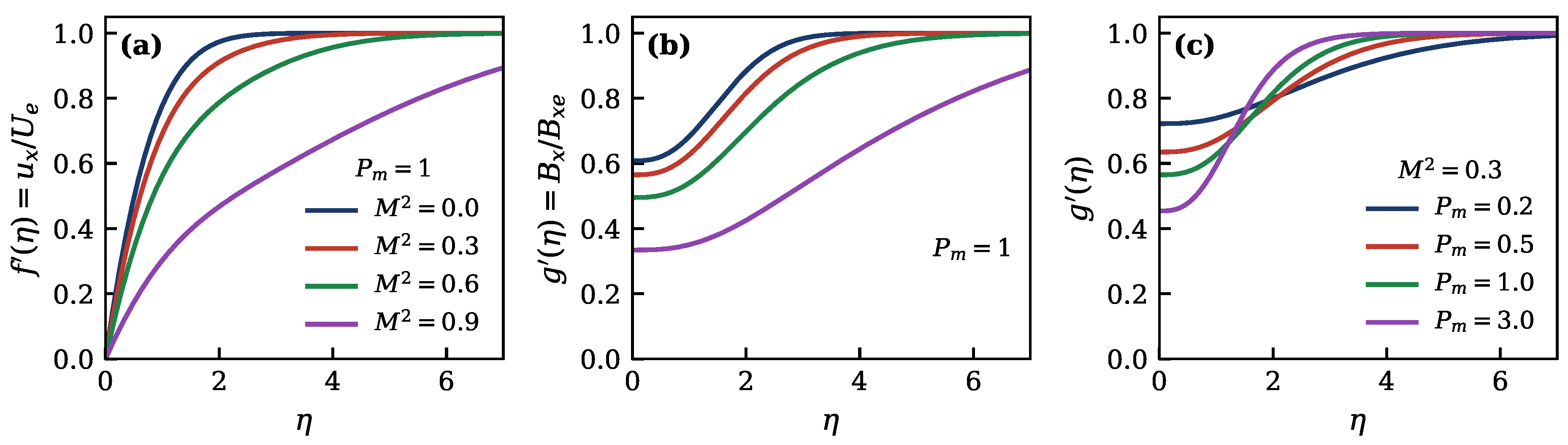
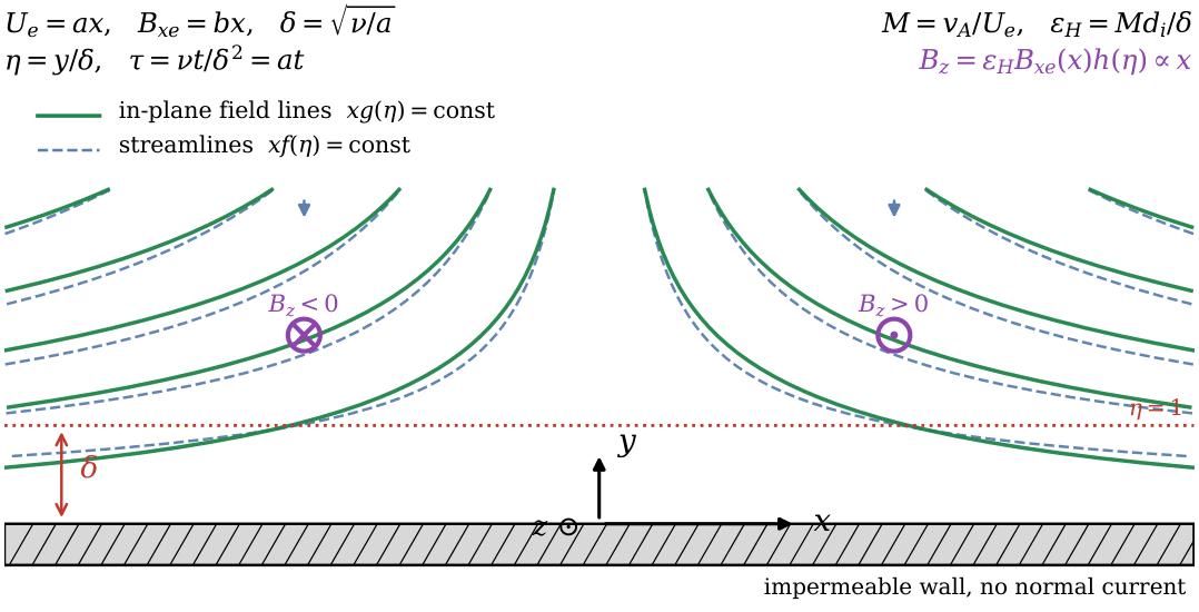
Figure 1 shows the geometry. Figure 2 gives the in-plane profiles: increasing M 2 thickens the velocity layer and reduces the wall stress, while increasing P m thins the magnetic layer relative to the viscous one, as expected from δ m / δ P m 1 / 2 . Note that g ( 0 ) 0 : the wall carries a finite tangential field, an output of the E 0 = 0 formulation rather than an imposed condition.
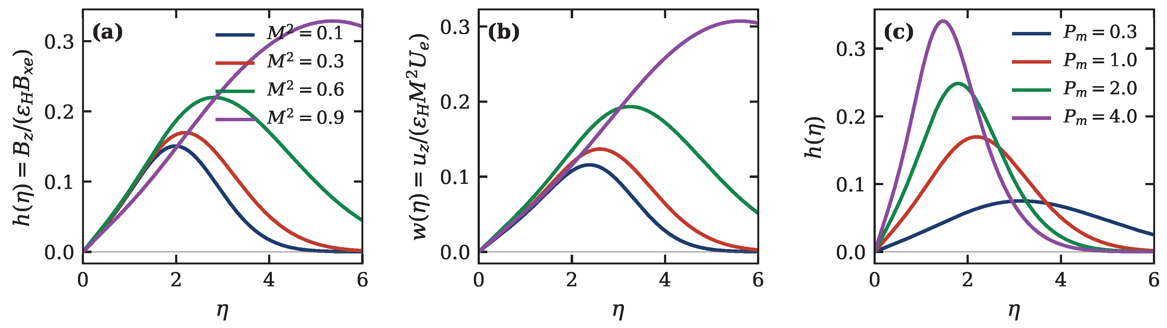
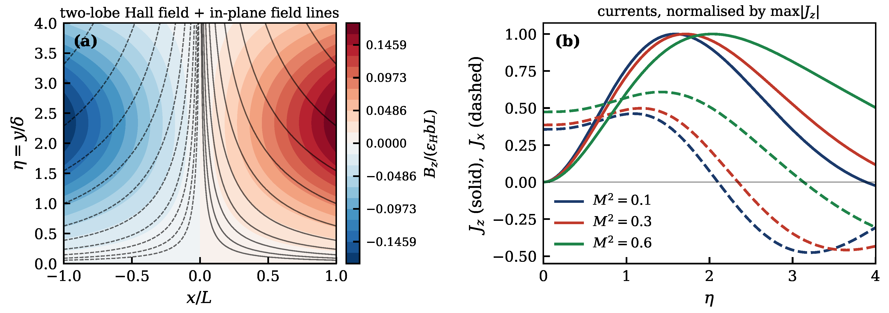
Figure 3 shows the Hall fields. Both h and w vanish at the wall and at infinity and peak near η 1.5 –2, i.e., near the outer part of the magnetic layer where η ( g η 2 g g η η ) is largest. The amplitude grows with M 2 and with P m , the latter because a thicker magnetic layer (small P m ) dilutes the source. Figure 4(a) displays B z in the physical plane together with the in-plane field lines, making the two-lobe structure explicit; panel (b) shows that J z g η η and J x h η peak at different heights and that J x reverses sign across the layer.

10.3. Verification of the O ( ε H 2 ) Hierarchy

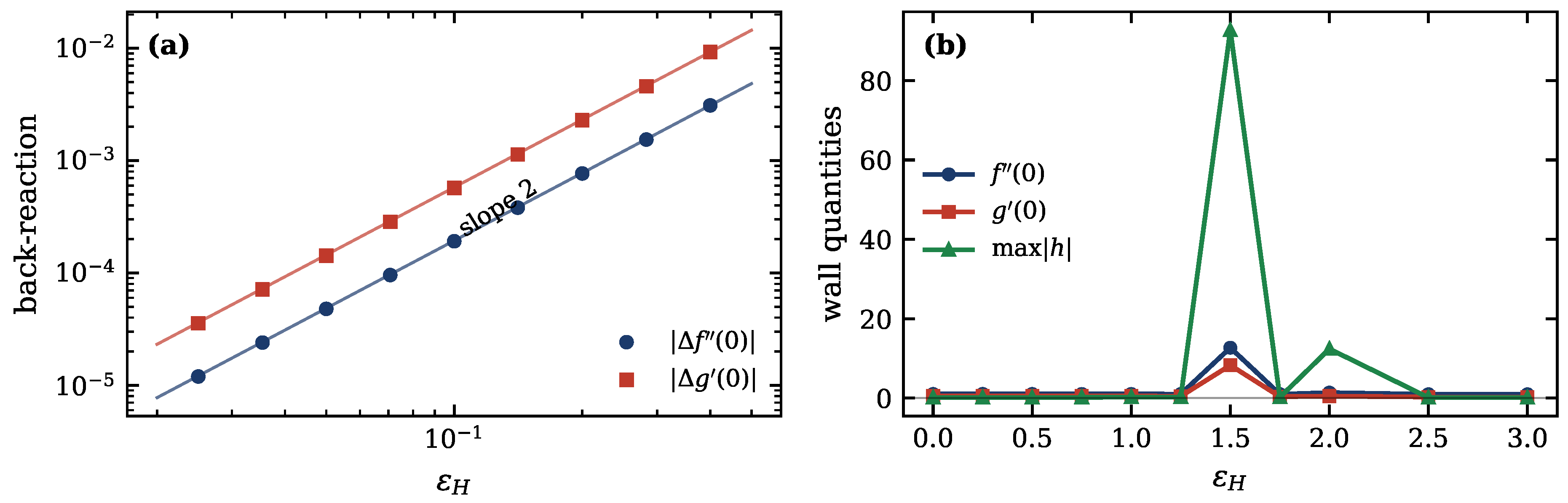
Figure 5(a) tests the central asymptotic prediction. Holding M 2 = 0.3 , P m = 1 and reducing ε H from 0.4 to 0.025 , the departures of the wall stress and wall field from their ε H = 0 values follow a clean power law of slope 2 over more than a decade, with prefactors converging to
| Δ f ( 0 ) | ε H 2 1.915 × 10 2 , | Δ g ( 0 ) | ε H 2 5.703 × 10 2 ,
while max | h | 0.169788 independently of ε H . This simultaneously confirms that the back-reaction is O ( ε H 2 ) and that the quadrupole shape is ε H -independent—the full hierarchy of Sec. 8 A.
Figure 5(b) extends the calculation beyond the perturbative regime, which is legitimate because Eqs. (50)–() are exact in ε H . Solutions continue smoothly to ε H 3 . The wall stress decreases only weakly, but the wall tangential field g ( 0 ) falls steeply and passes through zero near ε H 3.5 : at large Hall parameter the electron fluid slips so far from the ions that the tangential field at the wall reverses. The quadrupole amplitude is non-monotonic, peaking near ε H 1 and decreasing thereafter as the back-reaction suppresses the very gradients that generate it.

10.4. Dual-Temperature Structure

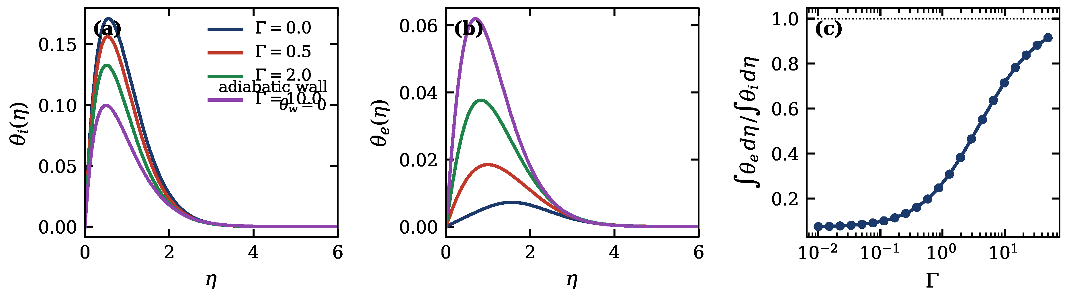
Figure 6 shows the thermal problem for an adiabatic-type wall condition θ w = 0 , so that all structure is generated internally by dissipation. At small Γ the ion and electron temperatures differ substantially: the ion profile is set by viscous heating and peaks close to the wall where f η η 2 is largest, whereas the electron profile is set by Ohmic heating g η η 2 and peaks farther out. As Γ increases the two profiles are driven together, and panel (c) quantifies the approach: the ratio of integrated excesses tends to unity as Γ , the single-temperature limit. The separation at small Γ is a direct consequence of the two-fluid dissipation split and is absent from any single-temperature model.

10.5. Class A and the Leading-Edge Region

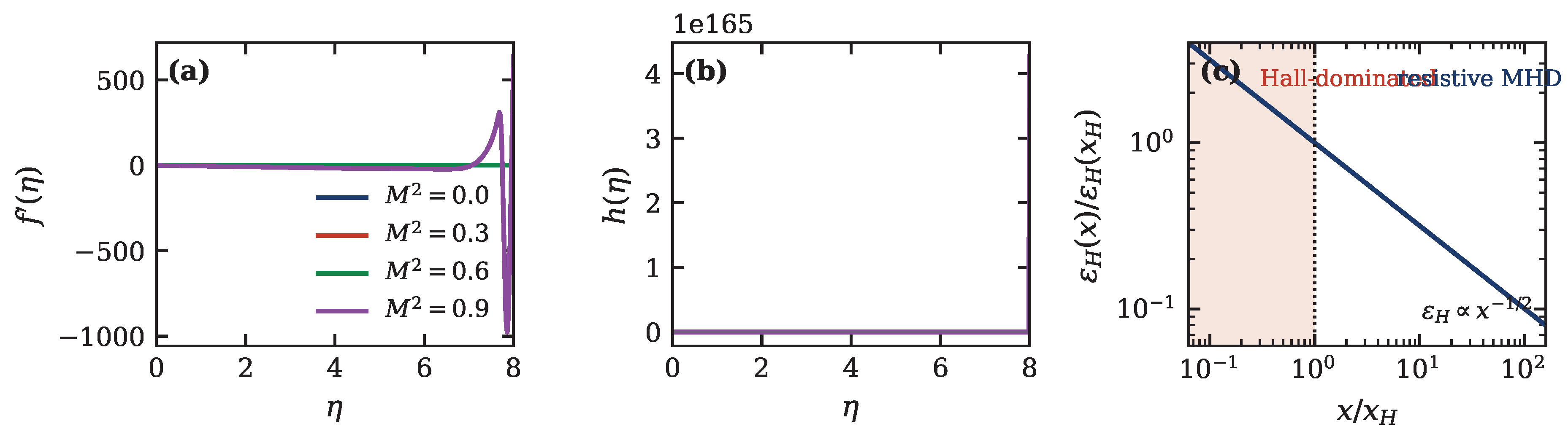
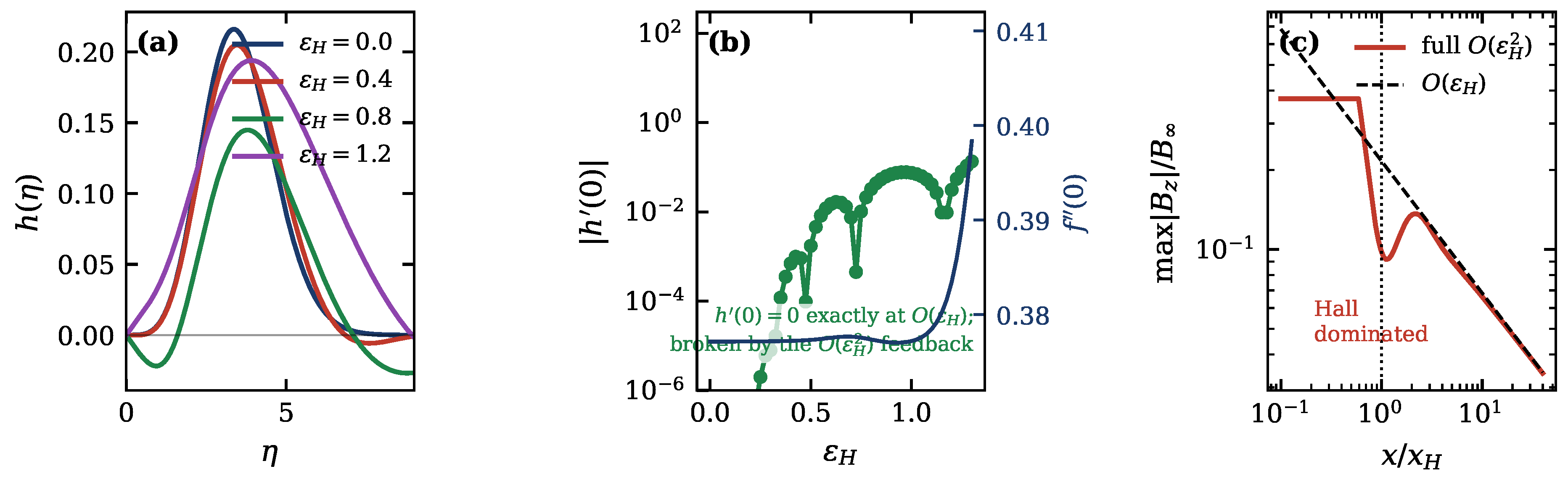
Figure 7 shows the Blasius-type layer at leading order. Figure 8 presents the full Class-A system with the O ( ε H 2 ) feedback retained. Panel (a) shows that the quadrupole profile h ( η ) is essentially ε H -independent up to ε H 0.4 —the numerical statement of Corollary 1—and distorts visibly only beyond ε H 0.8 . Panel (b) verifies the redundancy identified in Sec. 5 C: | h ( 0 ) | = 2 × 10 13 at ε H = 0 , i.e., machine zero, confirming that h ( 0 ) = 0 is an exact consequence of the divergence structure at O ( ε H ) ; it grows rapidly once the O ( ε H 2 ) feedback destroys that structure. The wall stress f ( 0 ) is remarkably insensitive to ε H in Class A, varying by under 6 % over 0 ε H 1.3 —far less than in Class B, because in Class A the feedback reaches the momentum equation only through the doubly indirect chain h g g g .
Panel (c) shows the downstream evolution. Using ε H ( x ) = ( x / x H ) 1 / 2 , the full solution follows the O ( ε H ) prediction max | B z | x 1 / 2 for x x H and departs from it upstream, where the layer is Hall dominated. We stress that panel (c) is a quasi-static (local-similarity) evaluation: at O ( ε H ) it is exact by Corollary 1, but at O ( ε H 2 ) the neglected streamwise-derivative terms enter at the same order, so the departure from the dashed line should be read as indicative rather than quantitative. The systematic treatment requires the second-order non-similar problem of Appendix D.

10.6. Approach to the Alfv énic Point

The exact degeneracy at M 2 = 1 , P m = 1 is approached continuously. Continuation in M 2 at P m = 1 , with η max enlarged as the layer thickens, gives
1 M 2 0.3 0.1 0.05 0.03 0.02 0.01
f ( 0 ) 0.7067 0.3936 0.2626 0.1919 0.1484 0.0944
α 1.533 3.247 5.110 7.055 9.027 13.41
The wall stress vanishes and the displacement thickness diverges as M 2 1 . The local logarithmic slope of f ( 0 ) drifts from 0.50 to 0.66 over this range; because α diverges simultaneously, a clean asymptotic exponent cannot be extracted from a finite domain, and we report only the qualitative degeneracy. The stability analysis below provides a much cleaner characterisation of the same limit.

10.7. Unsteady Evolution: Birth of the Quadrupole

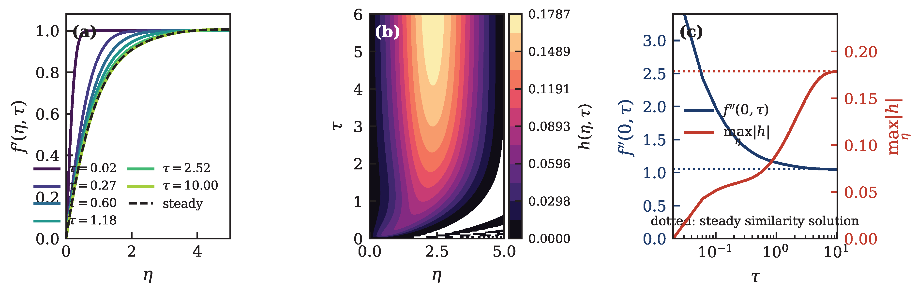
Figure 9 follows the impulsively started layer. At τ 1 the solution is the Rayleigh diffusive profile f η = erf ( η / 2 τ ) , with no Hall field. As τ grows, advection organizes the layer and the Hall source switches on; panel (b) shows h ( η , τ ) growing from zero, spreading outwards, and saturating on the similarity profile. Panel (c) records the wall stress and peak quadrupole amplitude relaxing onto the steady similarity values.
This calculation demonstrates that τ is a genuine similarity coordinate for Class B: the entire history from the diffusive to the convective regime collapses onto a single ( η , τ ) problem, with τ = a t carrying no residual x dependence. For Class A the corresponding variable is Stewartson’s τ = U t / 2 x , and the reduction retains the quasilinear terms 2 τ ( f τ f η η f η f η τ ) generated by D ; we show in Appendix B that these vanish identically on the Rayleigh solution, which is the correct small- τ limit, but that the coefficient of f η τ degenerates on the line 2 Λ τ f η = 1 , so that τ -marching is not globally admissible for Class A. This is a further, independent sense in which Class A is “less similar” than Class B.

11. Linear Stability of the Similarity States

11.1. Formulation

A similarity solution is physically meaningful only if it is an attractor. We therefore perturb the steady Class-B state,
f η = u 0 ( η ) + U ( η ) e σ τ , g = g 0 + G e σ τ , h = h 0 + H e σ τ , w = w 0 + W e σ τ ,
with F ( η ) = 0 η U d η , and linearize Eqs. (50)–(). The resulting operator is written out in Appendix E. Its boundary conditions are U ( 0 ) = U ( ) = 0 , G ( 0 ) = 0 , G η ( ) = 0 , H ( 0 ) = H ( ) = 0 , W ( 0 ) = W ( ) = 0 . At ε H = 0 the operator is block triangular— ( U , G ) autonomous, ( H , W ) slaved—so the spectrum is the union of the two block spectra; at finite ε H the blocks couple through the O ( ε H 2 ) term.

11.2. Results

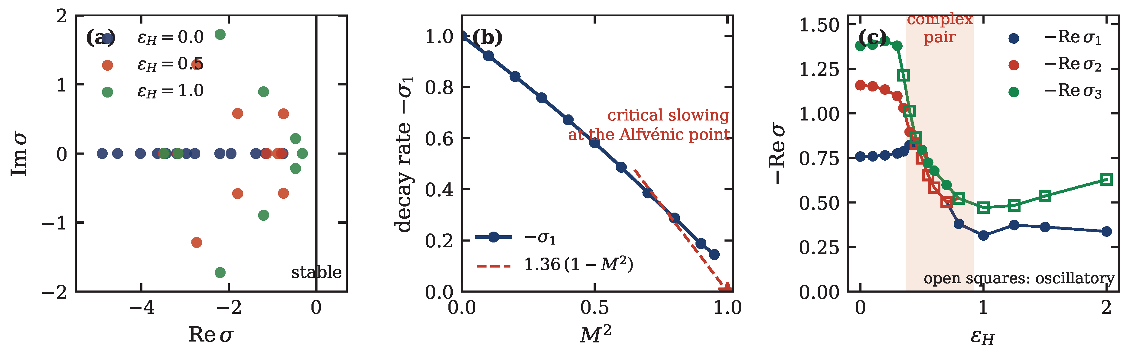
Figure 10(a) shows spectra in the complex σ plane. Every eigenvalue computed lies in the left half-plane, for M 2 0.95 , P m [ 0.5 , 2 ] and ε H 2 : the similarity states are linearly stable, and the numerical relaxation observed in Figure 9 is the generic behaviour, not a special initial condition.
Four quantitative results follow.
(i) An exact analytic eigenvalue. At M 2 = 0 we obtain
σ 1 = 1.00000000
to eight digits, and independently of P m . This is the displacement mode of Sec. 5.5: perturbing β at fixed α in Equation (71) gives δ β τ = δ β , hence σ = 1 exactly, for any P m . Analysis and computation agree to eight significant figures, which we regard as a stringent check on both.
(ii) Quantitative agreement with the unsteady solver. At M 2 = 0.3 , P m = 1 , ε H = 0 the leading eigenvalue is σ 1 = 0.75792 , converged to five digits under grid refinement ( N = 121 321 changes it by 8 × 10 5 ). Fitting the exponential decay of the difference between the unsteady PDE solution and the steady BVP solution over τ [ 4 , 11 ] gives a rate 0.76215 . The two differ by 0.6 % , and are obtained from solvers sharing no code. This identifies the relaxation rate observed in Sec. 10 G as the leading stability eigenvalue.
(iii) Critical slowing at the Alfvénic point.Figure 10(b) shows σ 1 decreasing monotonically with M 2 and vanishing linearly as M 2 1 ,
σ 1 1.36 ( 1 M 2 ) ,
fitted over M 2 [ 0.7 , 0.95 ] . The similarity state does not become unstable at the Alfvénic point; it becomes marginally stable, with the relaxation time diverging as ( 1 M 2 ) 1 . This is a far cleaner characterisation of the degeneracy than the drifting exponent of f ( 0 ) reported in Sec. 10 F, and it explains why the steady solver requires ever larger domains and tighter continuation as M 1 : the state it seeks is only weakly attracting.
(iv) Hall-induced oscillatory relaxation.Figure 10(c) tracks the three least-damped modes as ε H increases. Near ε H 0.4 two real eigenvalues collide and split into a complex-conjugate pair; at ε H = 0.5 the leading pair is σ = 0.7475 ± 0.575 i . Relaxation to the similarity state ceases to be monotone and becomes a damped oscillation. This is the whistler branch of Equation (92) appearing in the relaxation spectrum of the layer: a dispersive wave embedded in a dissipative structure. It is, to our knowledge, the cleanest dynamical signature of two-fluid physics available in a boundary-layer setting, and it is directly observable—an impulsively started Hall layer should ring at frequency | Im σ 1 | a rather than relax monotonically. Beyond ε H 0.9 the leading mode returns to the real axis as a different branch takes over.

11.3. Interpretation

The stability results tie the paper together. The σ = 1 mode is the displacement identity of Sec. 5.5 made dynamical. The critical slowing at M = 1 is the Alfvénic degeneracy of Sec. 4 C made quantitative. The complex pair at ε H 0.4 is the whistler dispersion relation of Sec. 8 C made observable. Each of the three structural features identified analytically appears independently in the spectrum of the linearised operator, which is the strongest internal consistency check we have been able to construct.

12. Limiting Cases and Consistency Checks

Because the reduced systems (50)–() and (55)–(58) contain five parameters, it is worth establishing explicitly that they collapse onto the classical problems in every accessible limit. Each check below is elementary, and together they constitute a complete audit of the reduction. We recommend that a reader reproducing this work verify them in the order given.

12.1. Hiemenz Flow: M 2 = 0 , ε H = 0

Setting M = 0 removes the magnetic terms from Equation (50), and the steady form becomes
f + f f + 1 f 2 = 0 , f ( 0 ) = f ( 0 ) = 0 , f ( ) = 1 ,
which is the Hiemenz stagnation-point equation. Our normalization δ = ν / a is the standard one, so the wall stress and displacement constant should be the tabulated values f ( 0 ) = 1.232588 , α = 0.647900 ; both are reproduced to six decimals (Table 3, first rows). Note that g remains coupled through Equation () as a passive scalar; this is why g ( 0 ) varies with P m in Table 3 even at M 2 = 0 .

12.2. Blasius Flow: Class A, M 2 = 0 , ε H = 0

Equation (55) reduces to f + f f = 0 . This is Blasius’ equation in the scaling δ = 2 ν x / U , related to the conventional η B = y U / ν x by η = η B / 2 and f = f B / 2 . Hence
f ( 0 ) = 2 f B ( 0 ) = 2 × 0.332057 = 0.469600 ,
and the displacement constant is 1.72079 / 2 = 1.216782 ; we obtain 0.469600 and 1.216781 . A reader who obtains 0.332 has used the other normalization; a reader who obtains 0.2348 has applied the factor twice.

12.3. Rayleigh–Stokes Layer: Class C, or Class B at τ 0

Class C has Λ = β ^ = 0 and Equation (50) collapses to f η τ = f η η η , i.e., t u x = ν y 2 u x , the one-dimensional diffusion equation with solution f η = erf ( η / 2 τ ) . The same profile is the correct small- τ limit of the impulsively started Class-B problem, since at early times the layer is too thin for advection to matter; this is why it is used as the initial condition in Sec. 10 G. Appendix B verifies that the nonlinear τ terms of the general reduction vanish identically on this solution.

12.4. Aligned-Field MHD: ε H = 0

At ε H = 0 the pair ()–() decouples and the in-plane problem is the classical aligned-field MHD boundary layer of Refs. [3,4,5]. Two independent checks apply. First, the Alfvénic degeneracy of Sec. 4 C: at M 2 = 1 , P m = 1 the state g = f forces f = 0 , so no boundary layer exists, and numerically f ( 0 ) 0 as M 2 1 (Sec. 10 F). Second, the displacement identity β = α of Equation (72), confirmed to six figures.

12.5. The Hall-Free Limit of the Four-Field System

Setting λ 0 (i.e., ε H 0 ) in Eqs. (18)–() leaves
t ψ + u · ψ = η m 2 ψ ,
with B z and u z satisfying homogeneous linear equations forced only by each other. With h ( 0 ) = h ( ) = w ( 0 ) = w ( ) = 0 the unique solution is h w 0 : no out-of-plane field is generated. This is the converse of Lemma 3 and a useful check that the source term has been retained with the correct coefficient—an error in the Hall coefficient would leave a spurious quadrupole in the resistive limit.

12.6. Single-Temperature Limit: Γ

Adding Eqs. (88) and () eliminates Γ , and in the limit Γ one has θ e θ i θ satisfying
θ τ = 1 2 1 Pr i + 1 Pr e θ η η + f θ η 2 f η θ + f η η 2 + M 2 P m g η η 2 + O ( ε H 2 ) ,
the standard single-fluid energy equation with a harmonic-mean conductivity and the total dissipation as source. Figure 6(c) exhibits this convergence numerically. Any formulation in which the two exchange coefficients differ fails this limit.

12.7. Summary of Checks

Table 4 collects the quantitative checks and the values obtained. We know of no further independent test that the present formulation passes only by construction.

13. Physical Mechanism of Quadrupole Generation

It is worth setting out, in words and in order, how the out-of-plane field is produced, because the algebra of Sec. 4 can obscure a simple chain of cause and effect.
Step 1: the primary current. The in-plane field is sheared by the layer, B x = B x e g η ( η ) with g η rising from g η ( 0 ) to unity. This shear is a current J z = μ 0 1 y B x , out of plane and concentrated in the magnetic layer.
Step 2: electron–ion slip. The current is carried predominantly by electrons, so u e differs from u by J / n e . The electrons therefore have an out-of-plane drift u e z = J z / n e relative to the ions, of order λ y B x .
Step 3: field-line stretching. Because the field is frozen to the electrons, the in-plane field lines are dragged in z by the differential electron drift. A field line threading the layer is stretched out of the plane at a rate B · u e z , generating B z . In similarity variables this is exactly the source
η g η 2 g g η η
of Equation (), which is nonzero wherever the electron drift varies along a field line.
Step 4: symmetry. The source is proportional to B x e ( x ) x in Class B, so B z x : positive on one side of the stagnation line, negative on the other. Reflecting in the wall-normal direction (as in a double-sided or reconnection geometry) gives the four-lobe quadrupole.
Step 5: the return flow. The Lorentz force μ 0 1 B · B z associated with the new field accelerates the ions in z, generating u z [Equation ()]. This in turn modifies the stretching in Step 3 through the M 2 ( g η w g w η ) term, closing an oscillatory loop—the whistler.
Step 6: back-reaction. Only now does the in-plane field feel the effect: the Hall term λ B · B z in Equation (29) transports flux, at relative order ε H 2 [Equation (38)].
The hierarchy of Sec. 8 A is precisely the statement that Steps 1–5 occur at O ( ε H ) and Step 6 at O ( ε H 2 ) . Steps 3 and 5 together constitute the whistler loop whose dispersion relation is Equation (92), whose numerical stiffness is Equation (97), and whose dynamical signature is the complex eigenvalue pair of Sec. 11. These are four descriptions of one mechanism.

14. Eigenfunctions and Wall Transpiration

14.1. Structure of the Leading Mode

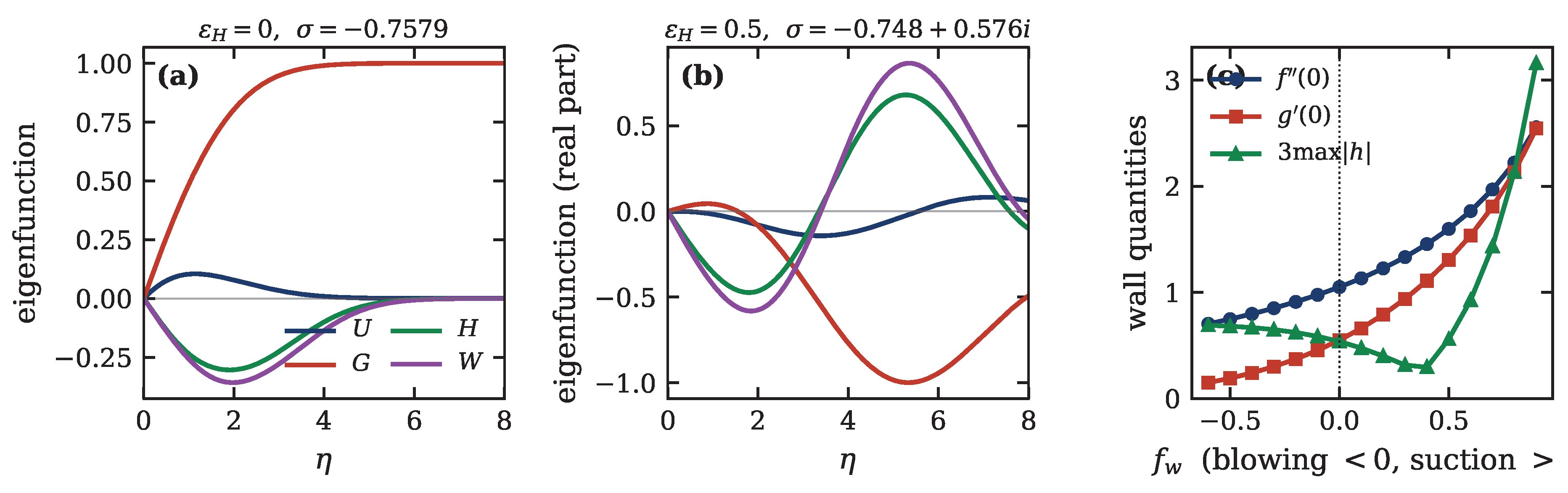
Figure 11(a) shows the leading eigenfunction at M 2 = 0.3 , P m = 1 , ε H = 0 . Its structure confirms the identification made in Sec. 11: the dominant component is G, which rises monotonically and tends to a nonzero constant as η , while U remains small and decays. This is exactly the displacement mode—a perturbation of the magnetic displacement constant β at nearly fixed α , relaxing according to Equation (71). At M 2 = 0 the identification is exact and σ = 1 ; at M 2 = 0.3 the mode acquires a small U component through the magnetic coupling and the eigenvalue shifts to 0.7579 .
Figure 11(b) shows the leading eigenfunction at ε H = 0.5 , where σ = 0.7476 + 0.5757 i . The character is entirely different: all four components are comparable, oscillate in η , and the out-of-plane pair ( H , W ) is as large as the in-plane pair. This is the whistler mode of Sec. 8 C rendered as a boundary-layer eigenfunction. The transition from panel (a) to panel (b) is the mode collision documented in Figure 10(c).

14.2. Wall Transpiration

The similarity structure admits one further physical parameter at no cost: a transpiring wall, f ( 0 ) = f w , with f w > 0 for suction and f w < 0 for blowing. This is compatible with Class B because u y ( 0 ) = a δ f w is independent of x, as the similarity form requires; it is the two-fluid analogue of the classical Hiemenz problem with suction.
Figure 11(c) shows the effect at M 2 = 0.3 , P m = 1 , ε H = 0.5 . Suction thins the layer and increases the wall stress and wall tangential field, as expected. More interesting is the quadrupole: max | h | increases by a factor of about five between f w = 0.6 and f w = + 0.9 , far more steeply than f ( 0 ) or g ( 0 ) . The reason is that the Hall source (108) depends on the curvature of the magnetic profile, which suction sharpens disproportionately. Wall transpiration is therefore an efficient experimental control on two-fluid effects in a boundary layer: a modest suction velocity produces a large change in the out-of-plane signature while leaving the in-plane flow comparatively undisturbed.

14.3. Thermal Parameter Study

Figure 12 completes the thermal picture.
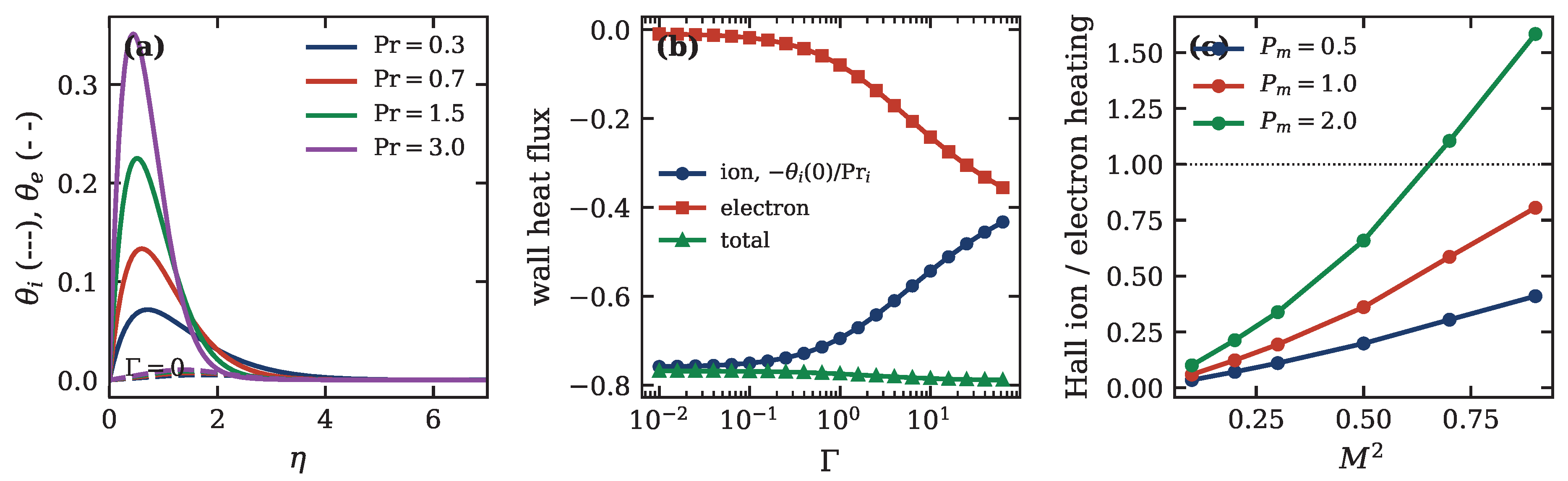
Panel (a) shows the effect of the Prandtl numbers with the species decoupled ( Γ = 0 ) and Pr i = Pr e = Pr . Increasing Pr confines the temperature rise closer to the wall and increases its peak, as in ordinary boundary layers, but the ion and electron profiles respond differently because their sources differ. At M 2 = 0.3 , P m = 1 the viscous source 2 f η η 2 substantially exceeds the Ohmic source ( 2 M 2 / P m ) g η η 2 , so the ion excess (solid) dominates the electron excess (dashed) by roughly an order of magnitude. The balance shifts towards the electrons at larger M 2 or smaller P m , both of which strengthen the Ohmic term.
Panel (b) shows the wall heat flux to each species as a function of the equipartition parameter. As Γ increases, the ion flux falls and the electron flux rises—equipartition transfers the viscously generated ion heat to the electrons, which then conduct it to the wall—while the total flux is nearly independent of Γ . This is the expected behaviour: the exchange term redistributes energy between species but neither creates nor destroys it, and the near-constancy of the total is a useful check on the implementation of Equation (80). The residual variation reflects the difference between Pr i and Pr e , which makes the two conduction paths to the wall unequal.
Panel (c) evaluates the Hall heating partition of Equation (77),
Hall ion heating Hall electron heating = P m M 2 w η 2 d η h η 2 d η ,
which measures how the additional dissipation introduced by two-fluid physics is divided. The ratio grows with both M 2 and P m and crosses unity near M 2 0.7 at P m = 1 . Below this the Hall contribution heats electrons preferentially (through the Hall current J x ); above it, ions (through the out-of-plane shear y u z ). Since the total Hall heating is O ( ε H 2 ) relative to the primary dissipation, this is a small correction in absolute terms, but it is the only channel by which two-fluid effects alter the partition of heating between species, and is therefore of direct interest for interpreting two-temperature measurements.

14.4. Benchmark Values

Table 5 lists high-precision values intended for verification of independent implementations. They were computed on η [ 0 , 16 ] with 2001 initial collocation nodes and tolerance 10 11 ; the last digit is uncertain at the level of a few units.

15. Relation to Reconnection Theory

The Class-B solution is not a reconnection solution: there is no X-line, no inflow of oppositely directed flux, and the wall imposes a boundary that a current sheet does not have. It is nevertheless worth setting out precisely which features are shared, because the quadrupole is normally introduced in the reconnection context and its appearance here is otherwise liable to be misread.
Shared features. (i) The generation mechanism is identical: differential electron drift along in-plane field lines, Steps 1–3 of Sec. 13. (ii) The symmetry is identical: B z x about the stagnation line, giving lobes of opposite sign, which upon reflection in the symmetry plane is the four-lobe quadrupole of Refs. [9,11,12]. (iii) The controlling parameter is the same ratio of d i to the layer thickness. (iv) The mediating wave is the whistler, with the same dispersion relation (92) and the same consequence that the dynamics is dispersive rather than Alfvénic at small scales [11].
Differences. (i) In reconnection the quadrupole amplitude is set by the reconnection rate and the ion diffusion region has thickness d i , so ε H = O ( 1 ) by construction; here ε H is an independent parameter and the theory is developed for arbitrary ε H . (ii) Reconnection geometry has B x 0 on the midplane, whereas here B x ( 0 ) = B x e g ( 0 ) 0 at the wall; the shear that drives the quadrupole is therefore boundary-driven rather than reversal-driven. (iii) The present problem is dissipative and possesses a stable steady state (Sec. 11), whereas the reconnection layer is intrinsically time-dependent.
What the present analysis adds. Because the geometry is a boundary layer, the problem admits an exact similarity reduction and hence exact statements that are unavailable in the reconnection setting: the quadrupole profile is a universal function h ( η ) independent of ε H (Sec. 4.3); the back-reaction on the in-plane field is rigorously O ( ε H 2 ) with computable prefactors [Equation (100)]; the whistler appears as a discrete complex eigenvalue of a linear operator (Sec. 11) rather than as a continuum branch; and the downstream fate of the quadrupole in a growing layer is fixed by Equation (61). These are, in our view, the aspects of the present work most likely to be useful outside the boundary-layer literature: the Class-B system is a clean, fully reducible testbed for Hall physics in which every structural statement can be checked exactly.

16. Applicability to Real Plasmas

16.1. Parameter Estimates

Table 6 evaluates the dimensionless groups for four representative systems using Braginskii transport coefficients [19,20], taking perpendicular coefficients wherever ω c s τ s > 1 . The estimates use δ = ν L / U for the collisional layer thickness and a = U / L for the strain rate.
Two robust features emerge. First, the ion Prandtl number is essentially universal:
Pr i = η 1 κ i / 3 2 = 0.225 ( ω c i τ i 1 ) , Pr i = η 0 κ i / 3 2 = 0.369
in the magnetized and unmagnetized limits respectively, both following directly from the ratios of Braginskii coefficients ( 0.3 / [ 2 / 1.5 ] and 0.96 / [ 3.9 / 1.5 ] ). It is not a free parameter. Second, the Alfvén number is close to unity, M 1.4 1.7 , for the Hall thruster, the reconnection experiment and the magnetopause—exactly the regime in which the magnetic group in Equation (50) is comparable to inertia, and in which the critical slowing of Sec. 11 is relevant.

16.2. Regime of Validity

The most consequential entry in Table 6 is ε H , which is large in every case. This is not an artefact of the parameter choices but a structural statement. Since ε H = M d i / δ and δ 2 = ν L / U ,
ε H 2 = M 2 d i 2 U ν L = M 2 Re L d i L 2 ,
so that
ε H 1 Re L L M d i 2 .
Collisional plasmas that are large compared with d i are also, generically, of high Reynolds number, and the two requirements conflict. The honest conclusion is that the collisional two-fluid boundary layer with ε H = O ( 1 ) occupies a restricted window, best approached by dense, relatively cold, moderately magnetized laboratory plasmas; the reconnection experiment, with ε H 7.5 and P m 1 , comes closest among the systems considered.
This does not render the theory inapplicable, for four reasons. First, Eqs. (50)–() are exact in ε H and we have shown that solutions exist up to ε H 3 , so the accessible range extends well beyond the asymptotic regime. Second, in a growing (Class A) layer ε H decreases downstream, so any such layer possesses a region where the theory applies, with the crossover located by Equation (61). Third, in systems where the layer width is set by anomalous rather than collisional transport, ν should be read as an effective diffusivity, typically orders of magnitude larger, which drives ε H down accordingly. Fourth, the classification theorem and the four degeneracies are statements about the structure of the equations and hold irrespective of parameter values.
What Table 6 does establish, and what we wish to state plainly, is that quoting small values of ε H for laboratory or space plasmas without such a qualification is not defensible.

16.3. Limitations

The model assumes constant density and incompressibility, which excludes the Biermann battery (Lemma 2), thermal-force and Nernst terms, and all compressional heating. It assumes isotropic scalar viscosity and conductivity, whereas a strongly magnetized plasma has strongly anisotropic Braginskii tensors, only partially captured by using perpendicular coefficients. It neglects electron inertia, so the electron skin depth d e and the associated sub- d i structure are absent; restoring d e would add a second inner scale and modify Equation (92) to ω 2 = k 2 v A 2 d i 2 k 2 / ( 1 + k 2 d e 2 ) at large k, removing the unbounded whistler frequency and, incidentally, the stiffness of Sec. 9 B. It is a laminar continuum theory, whereas layers with ε H 1 are frequently turbulent or collisionless. Finally, the stability analysis of Sec. 11 is restricted to perturbations of similarity form, i.e., to disturbances sharing the x-dependence of the base state; three-dimensional and streamwise-modulated disturbances (Tollmien–Schlichting and tearing branches) are not addressed.
The similarity classification of Theorem 1, by contrast, depends only on the structure of the transformation and on d i being an absolute length, and is therefore robust to all of these refinements.

16.4. Pitfalls in Planar Two-Fluid Formulations

It may be useful to collect, as a checklist, the degeneracies established above, each of which silently removes physics that a formulation may appear to contain:
1.
A Hall force written into the total momentum equation double counts J × B (Lemma 1).
2.
An electron-pressure term in the induction equation vanishes identically at constant density (Lemma 2); the two halves of Equation (11) must be kept or dropped together.
3.
A Hall term in the in-plane flux equation vanishes identically unless B z is retained (Lemma 3).
4.
The B z magnetic pressure cancels exactly from streamwise momentum (Lemma 4).
5.
The constraint B x e x is admissible only together with U e x , by Equation (33) and Theorem 1.
6.
The sign of the magnetic group in Equation (50) is fixed by the Alfvénic degeneracy.
7.
The Hall length in similarity units is ε H / M , linear in ε H .
8.
Energy consistency requires a single exchange coefficient Γ when both temperatures are normalized by the same scale.
9.
For Class A the perfectly conducting wall condition h ( 0 ) = 0 is redundant with far-field decay; the insulating condition h ( 0 ) = 0 is the non-degenerate choice.

17. Conclusion

We have derived the similarity structure of unsteady two-fluid plasma boundary layers from first principles, and found it to be governed by an obstruction with no single-fluid analogue.
The starting point is that a planar, constant-density two-fluid layer contains no Hall physics unless the out-of-plane field is retained: the Hall force cancels from total momentum, the electron-pressure term cancels from induction, the Hall term in the in-plane flux equation vanishes identically, and the B z magnetic pressure cancels from streamwise momentum. The minimal consistent model is the four-field system (18)–(20).
Under the map η = y / δ ( x ) , τ = ν t / δ 2 ( x ) the reduced system is autonomous only if the Hall group ε H = M d i / δ is constant. Because d i is an absolute length this forces δ = 0 , and Theorem 1 classifies the admissible families exhaustively. The stagnation-type layer U e = a x , δ = ν / a is exactly self-similar to all orders in ε H and yields the closed system (50)–() with the dual-temperature equations (88)–(); the Blasius-type growing layer is exactly self-similar through O ( ε H ) and breaks similarity only at O ( ε H 2 ) , its Hall subsystem collapsing to the first-order pair (58). The obstruction converts into the prediction that Hall physics in a growing layer is confined to a leading-edge region x H / d i = 1 2 M 2 Re d i .
The asymptotic hierarchy in ε H —resistive MHD at O ( 1 ) , a universal out-of-plane quadrupole at O ( ε H ) , back-reaction at O ( ε H 2 ) —was confirmed numerically over more than a decade in ε H , together with an exact identity between the viscous and magnetic displacement thicknesses and the degeneracy of the equipartitioned Alfvénic state. The Class-B solution reproduces the canonical Hall quadrupole of reconnection theory in a boundary-layer geometry, which we regard as the decisive check on the formulation.
The linear stability analysis shows the similarity states to be attractors, and supplies three independent confirmations of the analytical structure: an exact eigenvalue σ = 1 in the field-free limit, identified analytically as the displacement mode; a leading eigenvalue reproducing the measured relaxation rate of the unsteady solver to 0.6 % ; and critical slowing σ 1 1.36 ( 1 M 2 ) at the Alfvénic point. Above ε H 0.4 the leading pair becomes complex and relaxation turns oscillatory—the whistler branch entering the relaxation spectrum, and the most directly observable dynamical signature of two-fluid physics that this geometry affords.
Natural extensions include finite electron inertia, which introduces d e and removes the whistler stiffness; compressibility and the Biermann battery; anisotropic Braginskii closure; the second-order non-similar Class-A problem of Appendix D; and stability to streamwise-modulated and three-dimensional disturbances, for which the present analysis provides the base states.
Acknowledgment: My investigations into the boundary layers started from my tenure as a professor at the Cape Peninsula University of Technology (CPUT), South Africa. I am profoundly grateful to CPUT for granting me complete academic autonomy to advance this research agenda. This vital institutional support laid the foundation for the principal conclusions presented in this manuscript. I also extend my deepest gratitude to former Vice-Chancellor (now Chancellor) Prof. Brian Figaji, and former Deputy Vice-Chancellors Prof. J. A. Tromp and Prof. Anthony Staak, for their generous support and endorsement.
Further academic support was provided by Xi’an University of Architecture and Technology (XAUAT) and the Beijing Institute of Nanoenergy and Nanosystems (BINN), Chinese Academy of Sciences. I sincerely thank former XAUAT President Prof. Xiao-Jun Liu and current President Prof. Xiang-Mo Zhao, along with BINN Founding Director Prof. Zhong Lin Wang, for their unwavering encouragement and invaluable resource support throughout this study.
Conflict of interests: The authors declare that there are no competing financial interests.
Availability of data: The data supporting the findings of this study are available from the corresponding author upon reasonable request.

Appendix A Detailed Similarity Reduction

We give the substitutions in full. Throughout, primes on δ , U e , B x e denote d / d x ; subscripts η , τ denote partial derivatives.

Appendix A.1. Class B: Kinematics

With δ = ν / a constant, η = y / δ and τ = a t are independent of x, so x | y , t acts only on the explicit prefactors. From ϕ = U e δ f = a x δ f ,
u x = y ϕ = a x f η , u y = x ϕ = a δ f ,
and from ψ = b x δ g ,
B x = y ψ = b x g η , B y = x ψ = b δ g .
Note · u = a f η + ( a δ f ) η / δ · 0 is satisfied identically by construction.

Appendix A.2. Class B: Momentum

Each term of Equation (28):
t u x = a 2 x f η τ , u x x u x = a x f η · a f η = a 2 x f η 2 , u y y u x = a δ f · a x f η η δ = a 2 x f f η η , U e x U e = a 2 x , B x x B x = b x g η · b g η = b 2 x g η 2 , B y y B x = b δ g · b x g η η δ = b 2 x g g η η , B x e x B x e = b 2 x , ν y 2 u x = ν a x f η η η δ 2 = a 2 x f η η η .
Dividing by a 2 x and using M 2 = b 2 / ( μ 0 ρ a 2 ) gives Equation (50). Every term is proportional to x, which is why the reduction closes.

Appendix A.3. Class B: Flux Equation

t ψ = a b x δ g τ , u x x ψ = a x f η · b δ g = a b x δ f η g , u y y ψ = a δ f · b x g η = a b x δ f g η , λ B x x B z = λ b x g η · ε H b h = λ ε H b 2 x g η h , λ B y y B z = λ b δ g · ε H b x h η δ = λ ε H b 2 x g h η , η m y 2 ψ = η m b x g η η δ .
Dividing by a b x δ , the Hall coefficient is
λ ε H b 2 a b δ = ε H · λ b a δ = ε H 2 ,
and the resistive coefficient is η m / ( a δ 2 ) = η m / ν = 1 / P m , giving Equation ().

Appendix A.4. Class B: B z Equation

The Hall source requires y 2 ψ = b x g η η / δ , whence
λ B x x y 2 ψ = λ b x g η · b g η η δ = λ b 2 x δ g η g η η , λ B y y 3 ψ = λ b δ g · b x g η η η δ 2 = λ b 2 x δ g g η η η .
Dividing by a ε H b x gives coefficient λ b / ( a δ ε H ) = 1 , so the source is g η g η η g g η η η = η ( g η 2 g g η η ) . The stretching term, with u z = ε H M 2 a x w ,
B x x u z + B y y u z = b x g η · ε H M 2 a w b δ g · ε H M 2 a x w η δ = ε H M 2 a b x g η w g w η ,
divided by a ε H b x gives M 2 ( g η w g w η ) . Collecting yields Equation ().

Appendix A.5. Class B: U z Equation

The Lorentz term is μ 0 1 ( B x x B z + B y y B z ) = μ 0 1 ε H b 2 x ( g η h g h η ) ; dividing by ρ a · ε H M 2 a x gives
ε H b 2 μ 0 ρ a 2 ε H M 2 = M 2 M 2 = 1 ,
and the viscous coefficient is ν / ( a δ 2 ) = 1 , giving Equation (). This is the calculation that fixes the normalisation u z = ε H M 2 U e w ; any other choice leaves M 2 in two places instead of one.

Appendix A.6. Class A: Kinematics and the Divergence Structure

For Class A, δ = δ / 2 x 0 and D acts. Steadily,
u x = U f η , u y = U δ f + η f η , B x = B g η , B y = B δ g + η g η .
For the flux equation,
x ψ = B δ g η g η ,
so that
u x x ψ + u y y ψ = U B δ [ f η g η f η g η f g η + η f η g η ] = U B δ f η g f g η :
the η f η g η terms cancel, which is the mechanism by which Class A remains autonomous in the steady limit. Dividing by U B δ and using η m / ( U δ δ ) = 1 / ( Λ P m ) = 1 / P m gives Equation ().
For the out-of-plane fields we set B z = ε H ( x ) B h ( η ) with ε H x 1 / 2 , so that with B = ε H B x q , q = 1 / 2 ,
u x x B z + u y y B z = U B f η h U B δ δ f h η = U B x q f η h 1 2 f h η = U B 2 x η f h ,
using q = 1 / 2 and δ / δ = 1 / 2 x . This is the origin of the divergence form in Equation (57): it is a consequence of the exponent q = 1 / 2 , which in turn follows from ε H δ 1 x 1 / 2 . The Hall source reduces analogously to η ( g g η η ) and the stretching term to M 2 η ( g w ) , completing Equation (57).

Appendix B The General Non-Similar Momentum Equation

Retaining D , the streamwise momentum equation reduces to Equation (45). We record two properties.

Appendix B.1. Vanishing on the Rayleigh Solution

For Class A ( β ^ = 0 , Λ = 1 ) the bracketed nonlinear τ terms survive. Put f η = F ( s ) with s = η / τ and f = τ F ( s ) , F = F . Then
f τ = 1 2 τ F s F , f η η = F τ , f η τ = s F 2 τ ,
and therefore
f f η η + 2 τ f τ f η η f η f η τ = F F + F s F F + s F F = 0 .
The residual f η τ = f η η η becomes F + 1 2 s F = 0 , i.e., F = erf ( s / 2 ) : the Rayleigh solution, as required. This confirms both the algebra and the identification of τ 0 as the diffusive limit.

Appendix B.2. Degeneracy of τ-Marching

Rearranging Equation (45) for Class A,
1 2 Λ τ f η f η τ + 2 Λ τ f τ f η η = f η η η + Λ f f η η + M 2 ( ) .
The coefficient of f η τ vanishes on the line 2 Λ τ f η = 1 , which for Λ = 1 and f η 1 occurs at τ = 1 / 2 . Marching in τ at fixed η therefore degenerates, because lines of constant η cross the characteristics of the quasilinear operator. This is a coordinate, not a physical, singularity—the underlying ( x , y , t ) problem is regular—but it means that Class A must be integrated in physical variables or with a characteristic-respecting scheme. Class B is free of this difficulty precisely because Λ = 0 there and the bracket reduces to unity. It is a third independent sense, alongside the ε H obstruction and the wall-condition redundancy, in which Class A is the less similar of the two.

Appendix C Wall Electrical Models

Appendix C.1. Perfectly Conducting Wall

At a perfect conductor the tangential electric field vanishes. Ohm’s law (4) at the wall, where u = 0 , gives
E z ( 0 ) = η r J z ( 0 ) + λ B · B z 0 ,
E x ( 0 ) = η r J x ( 0 ) + λ J y B z J z B y 0 .
With B y ( 0 ) = 0 (the wall being a flux surface, g ( 0 ) = 0 ), Equation () reduces to
η r μ 0 y B z ( 0 ) λ μ 0 B z ( 0 ) x B z ( 0 ) = 0 .
In Class-B similarity variables the two terms scale as ε H and ε H 2 respectively, so at leading order h η ( 0 ) = 0 , with an O ( ε H 2 ) correction. Equation (A16) with B y ( 0 ) = 0 gives the Hall-corrected wall current (66).

Appendix C.2. Insulating Wall

At an insulator no current crosses the boundary, so J y ( 0 ) = 0 exactly. Since μ 0 J y = x B z and B z = ε H B x e ( x ) h ( η ) ,
x B z | 0 = ε H B x e h ( 0 ) ( Class A : ( ε H B ) h ( 0 ) ) ,
which vanishes if and only if h ( 0 ) = 0 , since B x e 0 in Class B and ε H 0 in Class A. This condition involves no expansion in ε H .

Appendix C.3. Redundancy for Class A

Integrating the first of Eqs. (57) from 0 to ,
h η P m + f h M 2 g w g g η η 0 = 0 .
At η , h , w 0 exponentially while f , g η , so all products vanish; at η = 0 , f ( 0 ) = g ( 0 ) = 0 . Hence h η ( 0 ) = 0 identically for every decaying solution, and condition (W1) supplies no information: the two-parameter family of decaying solutions is then fixed only by w ( 0 ) = 0 , leaving h ( 0 ) free. Condition (W2), h ( 0 ) = 0 , closes the problem. This degeneracy is specific to Class A: in Class B the advective terms f η h f h η are not a total derivative, no such integral identity exists, and both h ( 0 ) = 0 and h ( ) = 0 are independent.

Appendix D The O(ε H 2 ) Correction Problem

Writing f = f 0 + ε H 2 f 2 , g = g 0 + ε H 2 g 2 in Eqs. (50)–() and collecting at O ( ε H 2 ) gives the linear inhomogeneous system
L f f 2 f 2 + f 0 f 2 + f 2 f 0 2 f 0 f 2
+ M 2 2 g 0 g 2 g 2 g 0 g 0 g 2 = 0 , L g g 2 g 2 P m + f 0 g 2 + f 2 g 0 f 0 g 2 f 2 g 0
= g 0 h 0 g 0 h 0 ,
with homogeneous boundary conditions f 2 ( 0 ) = f 2 ( 0 ) = f 2 ( ) = 0 , g 2 ( 0 ) = g 2 ( ) = 0 . The right-hand side of Equation () is the Hall flux transport evaluated on the leading-order quadrupole. The prefactors quoted in Equation (100) are | f 2 ( 0 ) | and | g 2 ( 0 ) | .
For Class A the same expansion must be supplemented by the streamwise derivatives of the O ( ε H 2 ) terms, because ε H 2 x 1 there. Writing ζ = ε H 2 as the marching variable and noting x | y , t ( δ / δ ) ( η η 2 ζ ζ ) , the correction problem acquires terms proportional to ζ ζ of the same order as those retained. Consequently the local-similarity (quasi-static) evaluation used in Figure 8(c) is exact at O ( ε H ) but only indicative at O ( ε H 2 ) ; a systematic treatment requires marching the two-dimensional non-similar problem. We flag this explicitly rather than presenting the quasi-static curve as quantitative.

Appendix E The Linearised Stability Operator

With the decomposition (101) and F = 0 η U , linearising Eqs. (50)–() gives
σ U = U + F u 0 + f 0 U 2 u 0 U
+ M 2 2 g 0 G G g 0 g 0 G , σ G = G P m + F g 0 + f 0 G U g 0 u 0 G
ε H 2 G h 0 + g 0 H G h 0 g 0 H , σ H = H P m + F h 0 + f 0 H U h 0 u 0 H + M 2 G w 0 + g 0 W G w 0 g 0 W
+ η 2 g 0 G G g 0 g 0 G , σ W = W + F w 0 + f 0 W U w 0 u 0 W
+ G h 0 + g 0 H G h 0 g 0 H ,
where u 0 = f 0 η . Note that Equation () contains G through the last term, so the discretization must support third derivatives of G. The nonlocal operator F makes the U column of the Jacobian lower triangular.
At ε H = 0 the ( U , G ) block decouples from ( H , W ) , and the displacement mode of Sec. 5.5 is obtained analytically: taking U 0 (hence F 0 ) and G const = δ β as η , Equation () reduces in the far field to σ G = u 0 G = G , giving σ = 1 independently of P m , in agreement with Equation (102).

Appendix F Numerical Parameters

Steady solutions use collocation on η [ 0 , η max ] with η max = 10 –40 (enlarged near M 2 1 ), 900–2000 initial nodes, tolerance 10 9 , and continuation in M 2 , P m and ε H with step Δ ε H 0.05 ; larger steps fail to converge above ε H 1 , which accounts for apparent breakdowns reported from coarse continuation.
Unsteady solutions use N = 241 –641 uniform points on η [ 0 , 8 ] , second-order central differences in the variables ( u , G , h , w , θ i , θ e ) , and an implicit BDF integrator with banded Jacobian sparsity, relative tolerance 10 9 to 10 11 . Grid refinement from N = 241 to 481 changed the τ = 8 solution by less than 2 × 10 6 , confirming that the residual difference from the steady BVP at that time is the decaying transient rather than discretization error.
Stability spectra use N = 121 –321 points on η [ 0 , 10 ] ; the leading eigenvalue at M 2 = 0.3 , P m = 1 , ε H = 0 varies from 0.757998 at N = 121 to 0.757917 at N = 321 , i.e., by 8 × 10 5 .

Appendix G Braginskii Coefficients and the Parameter Table

For reproducibility we record the transport formulae used to construct Table 6. Temperatures are in eV, densities in cm 3 where indicated, and Z = 1 , μ = m i / m p , ln Λ = 10 .

Appendix G.1. Collision Times

From the NRL formulary [20],
τ i = 2.09 × 10 7 T i 3 / 2 μ 1 / 2 n i ln Λ Z 4 s ,
τ e = 3.44 × 10 5 T e 3 / 2 n e ln Λ Z 2 s ,
and the magnetization parameters are ω c i τ i , ω c e τ e with ω c i = Z e B / m i , ω c e = e B / m e .

Appendix G.2. Momentum Diffusivity

Braginskii’s ion viscosity has an unmagnetized (parallel) coefficient η 0 = 0.96 n i T i τ i and a perpendicular coefficient η 1 = 0.3 n i T i / ( ω c i 2 τ i ) . We use
ν = 1 m i n × η 0 , ω c i τ i < 1 , η 1 , ω c i τ i > 1 ,
capped by the unmagnetized value. This is a deliberate simplification: the true stress is a tensor with five coefficients, and a boundary layer with a wall-normal gradient samples a combination of them. The estimate is intended to place systems on a logarithmic scale, not to be accurate to better than a factor of a few.

Appendix G.3. Magnetic Diffusivity

The parallel Spitzer resistivity is
η = 1.03 × 10 4 Z ln Λ T e 3 / 2 Ω m ,
and η 1.96 η for Z = 1 ; we use η when ω c e τ e > 1 . Then η m = η r / μ 0 and P m = ν / η m .

Appendix G.4. Thermal Diffusivities

With χ s = κ s / ( 3 2 n ) ,
κ i = 3.9 n T i τ i m i , κ i = 2 n T i m i ω c i 2 τ i ,
κ e = 3.16 n T e τ e m e , κ e = 4.66 n T e m e ω c e 2 τ e .
The universal Prandtl numbers quoted in Equation (110) follow directly: in the magnetized limit
Pr i = η 1 / ( m i n ) κ i / ( 3 2 n ) = 0.3 2 / 1.5 = 0.225 ,
and in the unmagnetized limit Pr i = 0.96 / ( 3.9 / 1.5 ) = 0.369 . Both are independent of n, B and T; the ion Prandtl number of a Braginskii plasma is a pure number determined by which regime it is in.

Appendix G.5. Equipartition

The electron–ion energy equilibration rate is
ν ε e i = 3.2 × 10 9 Z 2 ln Λ n i μ T e 3 / 2 s 1 , τ Δ = 1 ν ε ,
whence Γ = 1 / ( a τ Δ ) with a = U / L . The very small values of Γ in Table 6 reflect the m e / m i mass-ratio suppression of equipartition: in all four systems the ion and electron temperatures in a boundary layer would remain distinct, which is the physical justification for retaining two temperatures at all.

Appendix G.6. Derived Groups

Finally
d i = m i μ 0 n e 2 Z 2 , v A = B μ 0 m i n , M = v A U ,
and, with a = U / L and δ = ν / a = ν L / U ,
ε H = M d i δ , Re L = U L ν , ε H 2 = M 2 Re L d i L 2 .
The last identity is Equation (111) and is the origin of the validity constraint discussed in Sec. 16 B.

Appendix H Reproduction Guide

This appendix records what is required to reproduce the results, in the order in which a reader is likely to want them.

Appendix H.1. Steady Class-B Solver

Represent the state as y = ( f , f , f , g , g , h , h , w , w , θ i , θ i , θ e , θ e ) and supply g , g , h through the elimination (94). The boundary conditions are Equation (70). Start from
f = g = η 1 + e η , f = g = 1 e η , h = w = 0 ,
at M 2 = ε H = 0 and continue in M 2 , then P m , then ε H . Continuation steps Δ ε H 0.05 are needed above ε H 0.8 ; larger steps diverge and can be mistaken for a genuine breakdown of the solution branch. The first checks to run are Hiemenz ( f ( 0 ) = 1.232588 ) and the identity β = α .

Appendix H.2. Unsteady Solver

Use u = f η and G = g η ; do not integrate g directly, or the far-field cancellation described in Sec. 9 B will dominate the error. The Hall source is evaluated as η Q with Q = 2 G η + G η 2 ( η + G ) G η η , which equals g η 2 g g η η 1 identically. Initialise at τ 0 = 0.02 with
u = erf η 2 τ 0 , g η = erf η 2 τ 0 / P m , h = w = 0 .
Starting at τ 0 = 10 3 fails: the Rayleigh layer is then thinner than a few grid cells and the third derivative in the Hall source is unresolved. Integrate with a stiff implicit method; explicit and IMEX schemes diverge for the reason given in Sec. 9 B, and the divergence appears first at η η max , which is a useful diagnostic that one has met the whistler constraint rather than a coding error.

Appendix H.3. Stability Solver

Assemble Eqs. (A23)–() as a dense matrix in the ordering ( U , G , H , W ) , with the nonlocal F = 0 η U represented by a trapezoidal lower-triangular matrix. Eliminate the Dirichlet nodes rather than penalising them; penalisation introduces spurious eigenvalues near the origin that are easily mistaken for physical slow modes. The Neumann condition on G at η max is imposed by a mirror ghost. Verify against σ 1 = 1 at M 2 = 0 , which must hold to machine precision for every P m .

Appendix H.4. Figures

Figure 2, Figure 3, Figure 5, Figure 6 and Figure 7 require only the steady solvers; Figure 9 the unsteady solver; Figure 10 and Figure 11 the eigenvalue solver; Figure 8 the Class-A system with feedback; and Figure 12 the steady solver with a thermal sweep. Total runtime is a few tens of minutes on a single core, dominated by the eigenvalue sweeps.

References

  1. H. Schlichting and K. Gersten, Boundary-Layer Theory, 9th ed. (Springer, Berlin, 2017).
  2. L. Rosenhead (ed.), Laminar Boundary Layers (Oxford University Press, Oxford, 1963).
  3. H. P. Greenspan and G. F. Carrier, The magnetohydrodynamic flow past a flat plate, J. Fluid Mech. 6, 77 (1959).
  4. W. R. Sears, Magnetohydrodynamic effects in aerodynamic flows, ARS J. 29, 397 (1959); see also Rev. Mod. Phys. 32, 701 (1960).
  5. W. R. Sears and E. L. Resler, Theory of thin airfoils in fluids of high electrical conductivity, J. Fluid Mech. 5, 257 (1959).
  6. R. J. Gribben, The magnetohydrodynamic boundary layer in the presence of a pressure gradient, Proc. R. Soc. A 287, 123 (1965).
  7. K. Stewartson, On the impulsive motion of a flat plate in a viscous fluid, Q. J. Mech. Appl. Math. 4, 182 (1951).
  8. B. H. Sun, Similarity solutions of a class of unsteady laminar boundary layers, Phys. Fluids 36, 083616 (2024).
  9. B. U. Ö. Sonnerup, Magnetic field reconnection, in Solar System Plasma Physics, edited by L. T. Lanzerotti, C. F. Kennel and E. N. Parker (North-Holland, Amsterdam, 1979), Vol. III, p. 45.
  10. T. Terasawa, Hall current effect on tearing mode instability, Geophys. Res. Lett. 10, 475 (1983).
  11. M. E. Mandt, R. E. Denton and J. F. Drake, Transition to whistler mediated magnetic reconnection, Geophys. Res. Lett. 21, 73 (1994).
  12. J. Birn et al., Geospace Environmental Modeling (GEM) magnetic reconnection challenge, J. Geophys. Res. 106, 3715 (2001).
  13. D. A. Uzdensky and R. M. Kulsrud, Physical origin of the quadrupole out-of-plane magnetic field in Hall-magnetohydrodynamic reconnection, Phys. Plasmas 13, 062305 (2006).
  14. Y. Ren, M. Yamada, S. Gerhardt, H. Ji, R. Kulsrud and A. Kuritsyn, Experimental verification of the Hall effect during magnetic reconnection in a laboratory plasma, Phys. Rev. Lett. 95, 055003 (2005).
  15. M. Yamada, R. Kulsrud and H. Ji, Magnetic reconnection, Rev. Mod. Phys. 82, 603 (2010).
  16. J. L. Burch et al., Electron-scale measurements of magnetic reconnection in space, Science 352, aaf2939 (2016).
  17. T. J. Schep, F. Pegoraro and B. N. Kuvshinov, Generalized two-fluid theory of nonlinear magnetic structures, Phys. Plasmas 1, 2843 (1994).
  18. R. Fitzpatrick and F. Porcelli, Collisionless magnetic reconnection with arbitrary guide field, Phys. Plasmas 11, 4713 (2004).
  19. S. I. Braginskii, Transport processes in a plasma, Rev. Plasma Phys. 1, 205 (1965).
  20. J. D. Huba, NRL Plasma Formulary (Naval Research Laboratory, Washington, DC, 2019).
  21. D. M. Goebel and I. Katz, Fundamentals of Electric Propulsion: Ion and Hall Thrusters (Wiley, Hoboken, 2008).
  22. H. B. Keller, Numerical methods in boundary-layer theory, Annu. Rev. Fluid Mech. 10, 417 (1978).
  23. P. Virtanen et al., SciPy 1.0: Fundamental algorithms for scientific computing in Python, Nat. Methods 17, 261 (2020).
  24. P. G. Drazin and W. H. Reid, Hydrodynamic Stability, 2nd ed. (Cambridge University Press, Cambridge, 2004).
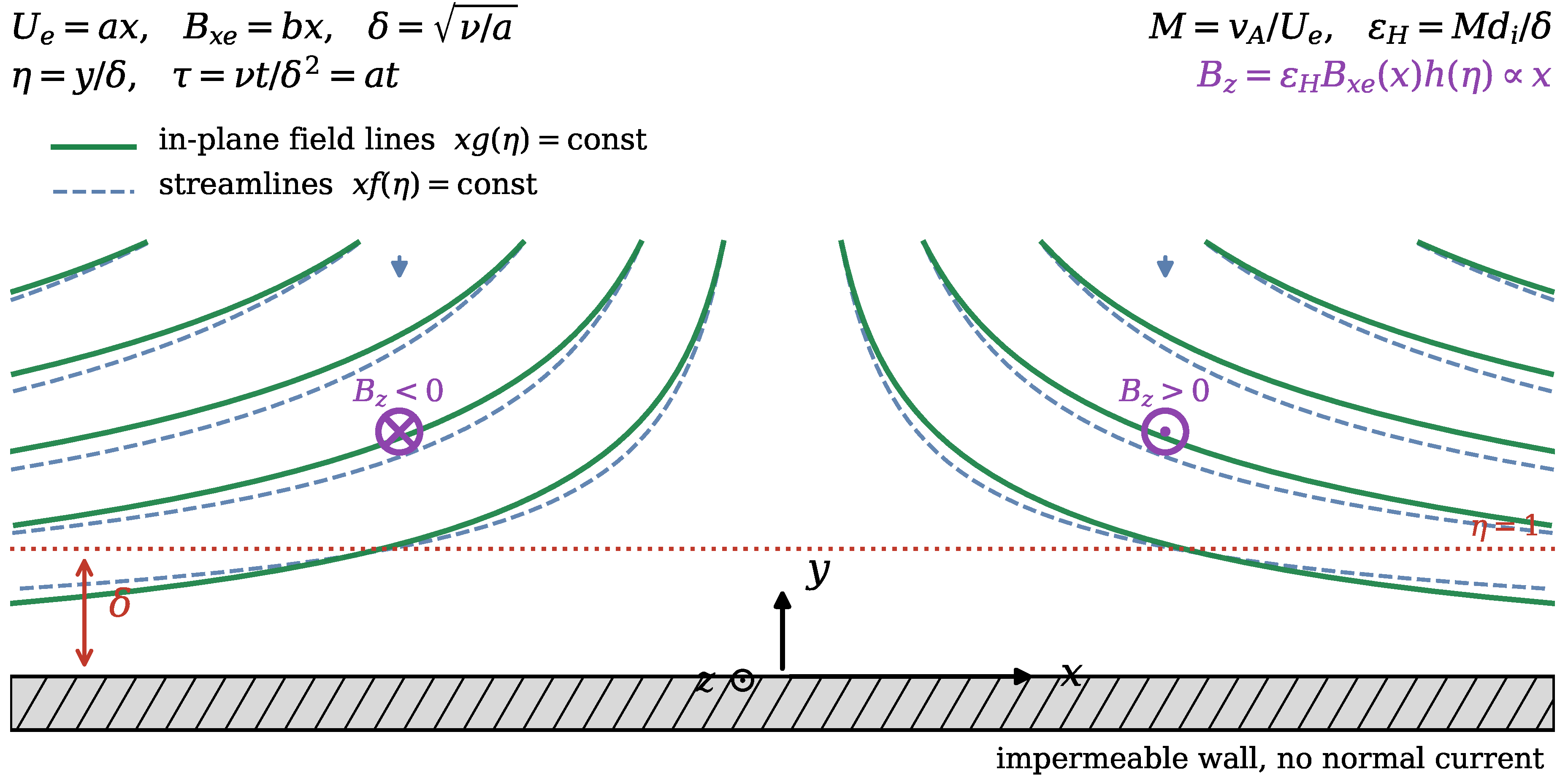
Figure 1. Geometry of the exactly self-similar (Class B) two-fluid boundary layer. Green curves are in-plane magnetic field lines x g ( η ) = const and dashed blue curves are streamlines x f ( η ) = const , both computed from the solution at M 2 = 0.3 , P m = 5 , ε H = 0.6 ; their separation is the magnetic boundary layer. The Hall-generated out-of-plane field B z = ε H B x e ( x ) h ( η ) x is antisymmetric about the stagnation line, forming the two-lobe (quadrupolar) structure marked ⊗/⊙.
Preprints 229960 g001
Figure 2. Steady Class-B base state. (a) Velocity profile f = u x / U e and (b) magnetic profile g = B x / B x e for several Alfvén numbers at P m = 1 . (c) Effect of the magnetic Prandtl number at M 2 = 0.3 .
Preprints 229960 g002
Figure 3. Hall-generated out-of-plane fields at leading order, independent of ε H . (a) h = B z / ( ε H B x e ) and (b) w = u z / ( ε H M 2 U e ) for several M 2 at P m = 1 ; (c) dependence of h on P m at M 2 = 0.3 .
Preprints 229960 g003
Figure 4. (a) Out-of-plane field B z x h ( η ) in the physical plane with in-plane field lines x g ( η ) = const superposed, showing the two-lobe Hall structure. (b) Normalized current densities: J z g η η (solid) and the Hall current J x h η (dashed), which reverses across the layer.
Preprints 229960 g004
Figure 5. (a) Departure of the wall stress and wall tangential field from their Hall-free values versus ε H at M 2 = 0.3 , P m = 1 . Solid lines have slope 2, confirming the predicted O ( ε H 2 ) back-reaction. (b) Continuation to finite ε H , where the reduced system remains exact: the wall field g ( 0 ) decreases steeply and reverses sign, and the quadrupole amplitude peaks near ε H 1 .
Preprints 229960 g005
Figure 6. Dual-temperature structure at M 2 = 0.3 , P m = 1 , ε H = 0.5 , Pr i = 1 , Pr e = 0.7 , with θ w = 0 so that all heating is internal. (a) Ion and (b) electron temperature profiles for several equipartition parameters Γ . (c) Ratio of integrated temperature excesses, approaching unity in the strongly coupled limit.
Preprints 229960 g006
Figure 7. Blasius-type (Class A) layer at leading order. (a) Velocity profiles; (b) universal Hall profile h ( η ) from the first-order system (58); (c) downstream decay ε H x 1 / 2 defining the leading-edge Hall region x x H of Equation (61).
Preprints 229960 g007
Figure 8. Class-A system with the O ( ε H 2 ) feedback retained, M 2 = 0.3 , P m = 1 . (a) Quadrupole profile, essentially ε H -independent up to ε H 0.4 and distorting beyond ε H 0.8 . (b) | h ( 0 ) | (green, left axis) is machine zero at ε H = 0 , verifying the divergence-form identity of Sec. 5 C, and grows once the O ( ε H 2 ) feedback breaks it; f ( 0 ) (blue, right axis) is nearly insensitive to ε H . (c) Downstream evolution of the quadrupole amplitude (quasi-static evaluation) against the O ( ε H ) prediction.
Preprints 229960 g008
Figure 9. Unsteady Class-B evolution from an impulsive (Rayleigh) start at M 2 = 0.3 , P m = 1 , ε H = 0.5 , Γ = 1 . (a) Velocity profiles at successive τ , converging on the steady similarity solution (dashed). (b) Growth and saturation of the Hall field h ( η , τ ) . (c) Wall stress and peak quadrupole amplitude versus τ ; dotted lines are the independently computed steady similarity values.
Preprints 229960 g009
Figure 10. Linear stability of the Class-B similarity states. (a) Spectra in the complex plane at M 2 = 0.3 , P m = 1 for three values of ε H ; all eigenvalues lie in the left half-plane. (b) Leading decay rate versus M 2 , vanishing linearly at the Alfvénic point as 1.36 ( 1 M 2 ) (dashed); the value at M 2 = 0 is exactly 1 , the analytically predicted displacement mode. (c) The three least-damped modes versus ε H : filled circles are real eigenvalues, open squares complex pairs. Near ε H 0.4 two real modes collide and relaxation becomes oscillatory (shaded).
Preprints 229960 g010
Figure 11. (a) Leading stability eigenfunction at M 2 = 0.3 , P m = 1 , ε H = 0 , normalized to unit maximum. The dominant component G tends to a constant at large η , identifying the mode as the magnetic displacement mode of Equation (71). (b) Leading eigenfunction at ε H = 0.5 , where the eigenvalue is complex: all four components are comparable and oscillatory, the whistler mode. (c) Effect of wall transpiration at ε H = 0.5 : the quadrupole amplitude responds far more strongly than the in-plane wall quantities.
Preprints 229960 g011
Figure 12. Thermal parameter study at M 2 = 0.3 , P m = 1 , ε H = 0.5 , θ w = 0 unless stated. (a) Ion (solid) and electron (dashed) temperature profiles for several Prandtl numbers with the species decoupled, Γ = 0 ; the ion excess dominates because the viscous source exceeds the Ohmic source at these parameters. (b) Wall heat flux to each species versus Γ : equipartition transfers heat from ions to electrons while the total is nearly conserved. (c) Hall heating partition, Equation (109), crossing unity near M 2 0.7 at P m = 1 .
Preprints 229960 g012
Table 2. Orders of magnitude in the boundary layer. ϵ = δ / L , ε H = M d i / δ , M = v A / U e .
Quantity Scale Relative order
u x U e 1
u y ϵ U e ϵ
B x B x e 1
B y ϵ B x e ϵ
B z ε H B x e ε H
u z ε H M 2 U e ε H M 2
J z B x e / μ 0 δ 1
J x ε H B x e / μ 0 δ ε H
J y ϵ ε H B x e / μ 0 δ ϵ ε H
Hall term in Equation (29) ε H 2
J y B z in Equation (23) ε H 2
Table 3. Steady Class-B similarity solutions at ε H = 0 . f ( 0 ) is the wall stress, g ( 0 ) = B x ( 0 ) / B x e the wall tangential field, α and β the viscous and magnetic displacement constants (predicted equal by Equation (72)), and max | h | , max | w | the quadrupole amplitudes.
M 2 P m f ( 0 ) g ( 0 ) α β max | h |
0.0 0.5 1.232588 0.676196 0.647900 0.647900 0.08868
0.0 1.0 1.232588 0.607950 0.647900 0.647900 0.14315
0.0 2.0 1.232588 0.537057 0.647900 0.647900 0.21709
0.1 1.0 1.178128 0.595312 0.699602 0.699602 0.15065
0.3 0.5 1.073318 0.634699 0.855213 0.855213 0.10867
0.3 1.0 1.054956 0.564698 0.839372 0.839372 0.16977
0.3 2.0 1.041246 0.494317 0.823716 0.823716 0.24842
0.5 1.0 0.904554 0.523006 1.068670 1.068670 0.19846
0.7 1.0 0.706677 0.459380 1.533259 1.533252 0.25104
0.9 1.0 0.394843 0.330920 3.170062 3.162032 0.38310
Table 4. Quantitative consistency checks.
Check Expected Obtained
Hiemenz f ( 0 ) 1.232588 1.232588
Hiemenz α 0.647900 0.647900
Blasius f ( 0 ) 0.469600 0.469600
Blasius displacement 1.216782 1.216781
β α 0 < 10 6
h ( 0 ) , Class A, ε H = 0 0 2 × 10 13
Back-reaction exponent 2 2.00
σ 1 at M 2 = 0 1 1.00000000
σ 1 vs. PDE rate equal 0.6 % apart
Rayleigh limit of Equation (45) 0 identically 0
Table 5. Benchmark values for the steady Class-B system. Pr i = Pr e = 1 , Γ = 0 , θ w = 1 (thermal quantities not listed).
M 2 P m ε H f ( 0 ) g ( 0 ) α max | h |
0.0 1.0 0.00 1.23258766 0.60795000 0.64790047 0.14315286
0.3 1.0 0.00 1.05495560 0.56469774 0.83937196 0.16976539
0.3 1.0 0.50 1.05013409 0.55024365 0.83191809 0.17884095
0.3 1.0 1.00 1.03371081 0.50040332 0.84551198 0.20051443
0.5 1.0 0.00 0.90455441 0.52300626 1.06867021 0.19845741
0.3 0.5 0.00 1.07331767 0.63469887 0.85521254 0.10866563
0.3 2.0 0.00 1.04124610 0.49431709 0.82371591 0.24842004
0.6 1.0 0.50 0.80068293 0.47563844 1.23281557 0.23475889
Table 6. Dimensionless groups from Braginskii transport, with δ = ν L / U . HT: Hall thruster channel ( n = 10 18 m 3 , B = 150 G, T e = 20 eV, Xe, L = 2.5 cm). MRX: laboratory reconnection ( n = 5 × 10 19 m 3 , B = 300 G, T = 10 eV, He, L = 10 cm). SOL: tokamak scrape-off layer ( n = 10 19 m 3 , B = 3 T, T = 30 eV, D, L = 1 cm). MP: magnetopause ( n = 2 × 10 7 m 3 , B = 30 nT, L = 10 3 km).
HT MRX SOL MP
d i (m) 2.6 6.4 × 10 2 1.0 × 10 1 5.1 × 10 4
δ (m) 5.0 × 10 3 1.3 × 10 2 9.3 × 10 6 3.3
M 1.68 1.54 293 1.46
ε H 8.8 × 10 2 7.5 3.2 × 10 6 2.3 × 10 4
P m 0.93 1.04 4.4 × 10 5 1.9
Pr i 0.369 0.225 0.225 0.225
Pr e 33 5.8 4.1 1.3
Γ 4.0 × 10 6 4.2 × 10 2 2.0 × 10 4 2.3 × 10 9
ω c i τ i 0.26 1.9 7.0 × 10 3 9.5 × 10 9
Re L 25 57 1.2 × 10 6 9.5 × 10 10
Disclaimer/Publisher’s Note: The statements, opinions and data contained in all publications are solely those of the individual author(s) and contributor(s) and not of MDPI and/or the editor(s). MDPI and/or the editor(s) disclaim responsibility for any injury to people or property resulting from any ideas, methods, instructions or products referred to in the content.
Copyright: This open access article is published under a Creative Commons CC BY 4.0 license, which permit the free download, distribution, and reuse, provided that the author and preprint are cited in any reuse.