

Submitted:
24 August 2026
Posted:
25 August 2026
You are already at the latest version
Abstract
As a common benign bone tumor, the pathological diagnosis of chondrogenic tumors needs to accurately analyze the calcification pattern of the cartilage matrix, key spatial topology information, and other important indicators. However, chondrogenic tumors is a rare disease, doctors lack sufficient reference data and experience in diagnosis. At the same time, complex spatial structural information also increases the difficulty of diagnosis, which leads to inconsistencies in the diagnosis’s results of different doctors. In contrast, with the development of technology, artificial intelligence (AI) with its fast, accurate, and robust characteristics can effectively improve the efficiency and accuracy of diagnosis. However, the application of AI in this field is still unrecognized, so it is urgent to develop a model that can help doctors in diagnosis to improve accuracy and efficiency. In this study, we propose XChondNet, an explainable spatial-context-aware synergistic deep feature fusion model for WSI-based chondrogenic tumor classification. The model proposes a fusion mechanism of pathological and positional features so that the model can effectively perceive spatial structural information and a parallel classifier mechanism based on potential coding, which can effectively solve the problem of class imbalance in chondrogenic tumors data. We evaluated the XChondNet model on our chondrogenic tumors dataset and the experimental results verified its effectiveness in the classification of the chondrogenic tumors subtype. In the test phase, compared to the other advanced models, the XChondNet model achieved state-of-the-art accuracy (ACC), area under the curve (AUC), F1 score and Recall rate. And the XChondNet model explicitly reflects the consistency with pathologists’ concerns, which improves the interpretability of AI.
Keywords:
feature fusion
; chondrogenic tumors
; digital pathology images
; tumor diagnosis
; parallel classifier mechanism
1. Introduction
Chondrogenic tumors is a relatively common benign bone tumor. However, there are many difficulties in diagnosis. First, it has a relatively low incidence compared to other bone tumors, such as osteochondroma accounting for 0.44(%) of all bone tumors [1]. As a result, clinicians have relatively little experience in diagnosis, making diagnosis difficult and prone to missed diagnosis or misdiagnosis. Secondly, the complex spatial structural information of the chondrogenic tumors leads to differences in evaluations among doctors. In addition, the limited number of experienced physicians has led to diagnostic delays and misdiagnosis in some cases. However, as technology advances, AI has been increasingly applied to WSI analysis, significantly improving pathological diagnostic performance. It has proven valuable in various tasks, including cancer subtype classification [2,3,4], tumor grading [5,6,7], prognosis analysis [8,9,10], gene mutation prediction [11,12,13]and image generation [14,15,16], improving markedly diagnostic efficiency and accuracy. Thus, AI provides new hope for solving the problem of chondrogenic tumors diagnosis, which can quickly and accurately identify pathological characteristics and provide strong support for doctors. Unlike many tumor classification tasks that mainly rely on local cellular morphology, chondrogenic tumor diagnosis requires the assessment of spatial tissue structures.
Figure 1 shows the lesion areas with spatial structural information for osteochondroma and subungual exostoses in the chondrogenic tumors subtype. Thus, capturing accurate spatial structural information is key to precise chondrogenic tumors diagnosis, but the current methods treat the internal area of the pathological image independently, without fully considering their spatial structural information in the original image and their relationship with each other.
To address this, we propose a XChondNet model for classifying chondrogenic tumors based on WSI, which provides a fusion mechanism of pathological and positional features, as well as a parallel classifier mechanism based on latent encoding. These effectively enable the model to perceive spatial structural information and solve data bias. The main contributions of this study can be summarized as follows:
- 1.
- As far as we know, we propose a robust pathological classification model for chondrogenic tumors for the first time.
- 2.
- Considering the pathological and positional characteristics of chondrogenic tumors, we propose a mechanism for fusing pathological and positional features, which effectively perceives spatial structural information.
- 3.
- Based on the uneven distribution of pathological data of chondrogenic tumors, we propose a parallel classifier mechanism.
- 4.
- The focus of XChondNet model is explicitly consistent with that of pathologists, enhancing AI transparency.
The structure of this paper is as follows: the Section 2 reviews the related works of pathological diagnosis in chondrogenic tumors and computational pathology, The Section 3 introduces the proposed method in detail, including the mechanism for fusing pathological and positional features, the parallel classifier mechanism and the Section 4 shows the experimental results and analysis, Finally, the Section 5 gives the conclusion.
2. Related Work
Due to morphological overlap and histological complexity, the diagnosis of enchondromas is challenging. In recent years, computational pathology and deep learning, particularly MIL-based methods, have shown promise in improving diagnostic accuracy. However, limitations remain in spatial structure modeling and data imbalance. This review summarizes relevant research from two perspectives: pathological diagnosis of enchondromas and computational pathology methods.
2.1. Pathological Diagnosis of Chondrogenic Tumors
Chondrogenic tumors comprise a heterogeneous group of lesions, including both benign and malignant tumors that typically affect bone tissue. Accurate diagnosis is crucial for developing personalized treatment plans and improving patient prognosis. However, the diagnosis of chondrogenic tumors remains challenging. Jesus-Garcia et al. [17] reported that although PET-CT can reflect metabolic activity, it cannot provide sufficiently clear evidence for distinguishing benign chondroma from chondrosarcoma, indicating the limitations of imaging examinations. Histopathology remains the gold standard for diagnosis, but it is also affected by morphological complexity. Wang et al. [18] discussed the diagnostic difficulty between low-grade chondrosarcoma and enchondroma, as both may show relatively benign chondrocyte morphology without obvious atypia or mitotic activity. Bansal et al. [19] further indicated that chondrogenic tumors need to be distinguished from non-chondrogenic lesions, such as synovial sarcoma, ectopic ossification, and calcified myositis, which may show similar matrix calcification or cell arrangement patterns.
Special histological subtypes also introduce diagnostic traps. Cates et al. [20] and Lan et al. [38] emphasized that chondroblastoma may be misdiagnosed as a malignant tumor because of its cellular polymorphism and nuclear groove characteristics. Schajowicz and Gallardo [21] reported that chondromyxoid fibroma, although benign and rare, often presents heterogeneous histological features such as myxoid matrix and pseudo-lobulated architecture, which may lead to diagnostic confusion. In addition, Bejnordi et al. [22] showed that differences in staining techniques may affect histopathological image analysis, and variability in pathologists’ experience may further influence diagnostic consistency.
With the development of artificial intelligence, deep learning methods have shown great potential in pathological image analysis. Lucas et al. [23] applied deep learning to automatic Gleason pattern classification, while Raees and Thomas [24], Wang et al. [25], and Zhang et al. [26] demonstrated the effectiveness of deep learning in medical image detection and classification tasks. These studies suggest that AI-based methods can provide consistent and efficient diagnostic support, reducing the influence of limited clinical experience and inter-observer variability. Therefore, deep learning has great potential to improve the diagnosis of chondrogenic tumors.
2.2. Computational Pathology
In recent years, the proposal and application of deep learning neural networks have greatly improved the performance of AI in medical prediction tasks, and with the continuous advancement of technology, significant improvements have also been made in the diagnosis and treatment of diseases such as cancer. This indicates the significant achievements made in the field of histopathology over the years of development.
In view of the excellent performance of convolutional neural networks (CNNs), many studies have used CNN-based methods or transfer learning techniques for histopathological image classification. De Matos et al. [27] segmented histopathological images into small patches, extracted features using Inception-V3, and combined SVM classifiers for patch screening and classification. Saxena et al. [28] used multiple pretrained CNN models as feature extractors for breast cancer histopathology diagnosis. Nazeri et al. [29] proposed a two-stage CNN framework, where the first stage extracted patch-level features and the second stage learned higher-level image representations for classification.
Due to the extremely high resolution of WSIs, multiple instance learning (MIL) has become a widely used framework for WSI-level classification. Carbonneau et al. [30] provided a comprehensive survey of MIL problem settings and applications. Ilse et al. [31] introduced attention-based deep MIL, enabling the model to learn the contribution of different instances to bag-level prediction. Lu et al. [3] proposed CLAM, which uses attention-based learning and clustering constraints to identify discriminative regions in whole-slide images. Li et al. [32] proposed DSMIL, which jointly models instance-level and bag-level representations through a dual-stream MIL framework. Shao et al. [33] introduced TransMIL by using Transformer-based correlation modeling among instances. Tang et al. [37] proposed MHIM-MIL to improve attention-based MIL through masked hard instance mining, and Tang et al. [35] further improved WSI classification through robust feature re-embedding. Xie et al. [36] proposed PHIM-MIL, which constructs hierarchical feature representations for WSI classification. These studies demonstrate the effectiveness of deep learning and MIL-based frameworks in computational pathology, but spatial structural information and data imbalance remain insufficiently explored for chondrogenic tumor diagnosis.
In summary, although deep learning models have achieved encouraging results in medical image analysis, especially in tissue pathology image classification, there are still limitations in dealing with the spatial structural information problems. Taking chondrogenic tumors classification as an example, tissue structure characteristics are crucial in diagnosis. For example, the diagnosis of osteochondroma requires attention to obvious pathological manifestations such as the periosteum, cartilage, and mature bone structures. And this model also needs to effectively address the challenge of an imbalanced dataset of chondrogenic tumors. However, existing technologies overlook these factors. Based on this, it is urgent to propose a suitable method for the chondrogenic tumors that can perceive spatial structural information and handle data imbalance.
3. Method
3.1. Notation and Problem Formulation
Given a whole-slide image (WSI), we represent it as a bag of image patches , where denotes the i-th patch and N is the number of patches in the WSI. The spatial coordinate of is denoted as , where and are the row and column coordinates, respectively. A pretrained pathological feature extractor maps each patch into a pathological feature vector . In this study, pathological features refer to the high-dimensional visual representations extracted from H&E-stained pathological image patches by a pretrained histopathology feature extractor. These features encode local tissue morphology, cellular arrangement, texture patterns, cartilage matrix characteristics, calcification-related structures, and other discriminative visual cues associated with chondrogenic tumor diagnosis. The positional encoding module maps into a positional feature vector . The fused patch representation is denoted as .
For slide-level classification, each WSI is associated with a slide-level label , where K denotes the number of tumor categories. In this study, , corresponding to OC, ED, CF, SE, CB, and CD. The goal of XChondNet is to learn a slide-level prediction from the patch-level fused representations .
3.2. Overview
The framework of the proposed model is shown in Figure 2. First, in the data acquisition stage, the tissue samples undergo decalcification, dehydration, transparency, wax immersion, H&E staining, sealing and microscopic observation for about 3 days to form the H&E stained sections we need. Due to the rare quantity of each category in the dataset, we annotated the corresponding regions of interest (ROI) through the professional pathologist from Tianjin hospital in China and obtained the ROI after processing the whole pathological section. In the data preprocessing stage, OTSU [39] algorithm is used to separate tissue regions. The positional information are recorded. Then the pathological features is extracted from the pathological image through the pre-trained model, and the position features are formed through the position coding module, and the pathological features is fused with the positional features. Finally, in the prediction stage, the multi-scale feature enhancement network and the parallel classifier mechanism are used to make predictions and generate heatmaps. The design of XChondNet is motivated by the pathological characteristics of chondrogenic tumors. Unlike many general WSI classification tasks that mainly rely on local cellular morphology, chondrogenic tumor diagnosis requires the assessment of spatial tissue organization, such as the arrangement of fibrous membrane, cartilage, and bone-related regions. Therefore, positional information is incorporated into pathological feature representation to help the model capture spatial structural cues. In addition, because some chondrogenic tumor subtypes are rare and the dataset is imbalanced, a parallel classifier mechanism is designed to enhance category-specific discrimination.
3.3. Data Preprocessing
After tissue segmentation by the OTSU algorithm, each WSI is divided into non-overlapping patches using a sliding-window strategy. The resulting WSI bag is represented as:
where denotes the i-th image patch, denotes its spatial coordinate, s is the patch size, and N is the number of patches in the WSI. This formulation keeps the pathological image patch and its corresponding spatial coordinate explicitly paired, which facilitates subsequent positional feature construction and feature fusion.
3.4. Mechanism of Fusion between Pathological Features and Positional Features
To capture the spatial structural information of chondrogenic tumors, XChondNet integrates pathological features and positional features at the patch level. This module consists of pathological feature extraction, positional feature construction, feature fusion, and multi-scale feature enhancement.
3.4.1. Extracting Pathological Features and Positional Features
For each patch , the pathological feature represents the morphology-related visual information extracted from the H&E-stained tissue region, including cell distribution, matrix texture, cartilage-related appearance, and ossification- or calcification-related patterns.
For each patch , a pretrained pathological feature extractor is used to obtain the patch-level pathological feature:
where denotes the pretrained pathological feature extractor and is the feature dimension.
To encode spatial information, the original coordinate is first normalized according to the spatial extent of the tissue region:
where is a small constant used to avoid division by zero.
The normalized coordinates are then transformed into high-dimensional positional embeddings through sinusoidal positional encoding. For each dimension t, the row-coordinate encoding is defined as:
and the column-coordinate encoding is defined similarly:
The final positional feature is obtained by concatenating the row and column positional embeddings:
where denotes the positional feature of the i-th patch.
3.4.2. Feature Fusion
The pathological feature and positional feature are concatenated and projected into a unified latent space:
The fused patch representations of all patches are denoted as:
3.4.3. Multi-scale Feature Enhancement Network
The multi-scale feature enhancement network is designed to strengthen discriminative patch representations and improve slide-level classification. It includes a gated attention module, an instance evaluation module, a region-aware weighting module, and a prototype-based contrastive regularization module.
3.4.3.1. Gated Attention Module.
Given the fused feature matrix , a gated attention mechanism is used to estimate category-aware patch importance:
where and denote the nonlinear feature branch and the gating branch, respectively, ⊙ denotes element-wise multiplication, and denotes the category-aware attention weights. The softmax operation is performed over the patch dimension for each class.
3.4.3.2. Instance Evaluation Module
To enhance instance-level discrimination, we select high-attention and low-attention patches according to the category-aware attention weights. For the ground-truth class , the positive and negative instance sets are defined as:
where is the number of selected instances. The selected instances are then used for instance-level supervision.
3.4.3.3. Region-aware Feature Weighting Module
A region-aware weight is further generated to describe the importance of each patch in the feature space:
The final slide-level representation for each category is obtained by combining category-aware attention and region-aware weights:
The category-specific slide representations are denoted as:
3.4.3.4. Prototype-based Contrastive Regularization Module
For prototype-based feature regularization, we define a learnable prototype matrix , where each row corresponds to a class prototype. The category-specific representations are first aggregated into a global slide representation:
The similarity between the slide-level representation and class prototypes is computed as:
where denotes L2 normalization, is the temperature parameter, and denotes the prototype similarity logits.
3.5. The Parallel Classifier Mechanism
Due to the rarity of chondrogenic tumors, the dataset shows obvious category imbalance. To reduce mutual interference among different categories, XChondNet adopts a parallel classifier mechanism, where each category is assigned an independent classifier. This design encourages each classifier to focus on category-specific discriminative features.
Given the category-specific representation , the logit of the k-th class is computed as:
where and are the parameters of the k-th classifier. The logits of all categories are collected as . The final slide-level probability is obtained by:
3.6. Attention-Based Interpretability Analysis
The interpretability of XChondNet is derived from its intrinsic category-aware attention mechanism. Specifically, patch-level attention scores are used to estimate the relative contribution of different tissue regions to the slide-level prediction, and these scores are mapped back to their original spatial positions to generate attention heatmaps.
Given the fused patch representation matrix , XChondNet first calculates the gated attention representation:
where ⊙ denotes element-wise multiplication, and denotes the sigmoid activation function. The category-aware attention weights are then obtained by:
where denotes the attention weight matrix, N is the number of patches, and K is the number of tumor categories. The softmax operation is performed along the patch dimension for each category, so that the attention weights reflect the relative importance of different patches for a specific class.
For the predicted class , the attention score of the i-th patch is defined as:
To generate the heatmap, the attention scores are normalized to the range of 0 to 1:
where is a small constant used to avoid division by zero. The normalized attention score is then assigned to the original spatial coordinate of the corresponding patch:
Finally, the attention map is converted into a color heatmap and overlaid on the original WSI. Regions with higher attention scores indicate tissue regions that contribute more strongly to the slide-level prediction, thereby providing visual evidence for the diagnostic decision of XChondNet.
3.7. Loss Function
The overall training objective consists of the slide-level classification loss, the instance-level loss, and the prototype contrastive loss:
The slide-level classification loss is defined as:
where is the one-hot slide-level label, and is the predicted probability distribution.
For instance-level supervision, the selected positive and negative instances are optimized using binary cross-entropy:
where denotes the set of selected instances, is the pseudo-label of the selected instance, and is the predicted probability of the instance classifier.
The prototype contrastive loss is defined as:
where denotes the prototype similarity logit for the k-th class.
4. Experiments
4.1. Data Acquisition
In this study, we used the H&E staining chondrogenic tumors dataset provided by Tianjin hospital in China, which is composed of uncompressed WSIs. The dataset was derived from archived samples of 228 patients with chondrogenic tumors from January 2017 to September 2024. The magnification of the image is 20 times, the corresponding pixel resolution is , and the size of each slice is different. Due to poor staining in some sections caused by their age, which affected image quality, we screened 264 samples.After screening, 139 samples were finally determined to be available for this study. The storage space requirement of the whole dataset is about 305GB, which covering six different types of chondrogenic tumors: osteochondroma(OC), enchondroma(ED), chondromyxoid fibroma(CF), subungual exostosis(SE), chondroblastoma(CB), and chondrosarcoma(CD). Examples of six subtypes of chondrogenic tumors lesions are shown in Figure 3.
In view of the limited number of samples in the dataset, we annotated the ROI in the WSIs by professional pathologists in Tianjin hospital, and extracted 1472 ROIs from them for experiments. To deal with the imbalance of categories in the dataset, and ensure the comprehensiveness of model training and the reliability of evaluation results, we used the 5-fold cross validation method to divide the dataset into the training set, the validation set and the test set. The ratio of each patient level was set as 8:1:1. In this process, we ensured that all samples of the same patient were assigned to the same subset. Taking the first fold cross validation as an example, we allocated 1147 ROIs for the training set, 162 ROIs for the validation set, and 163 ROIs for the test set. The specific division of the dataset is shown in Table 1.
4.2. Experimental Details
During training, XChondNet was optimized using the Adam optimizer with an initial learning rate of 0.001 and a weight decay of .The size of the small batch is 1. The classifier will verify the dataset every 200 epochs trained, and apply the early stop mechanism to finally test the test set. ACC, AUC, F1 score, Recall and Precision were used as experimental evaluation indicators. All experiments were performed on two NVIDIA RTX 3090 GPU computers.
4.3. Experimental Evaluation Indicators
This paper uses ACC, AUC, F1 score, Recall and Precision as evaluation indicators.
Accurate prediction of proportion image is called accuracy. It is indicated as follows:
The accuracy rate is measured by calculating the proportion of correct judgment of the model in all predictions, in which the true case (TP), the true negative case (TN), the false positive case (FP) and the false negative case (FN) are expressed by their abbreviations respectively.
AUC is an indicator calculated based on receiver operating characteristic curve. The ROC curve is drawn with the false positive rate (FPR) as the horizontal axis and the true positive rate (TPR) as the vertical axis. The value of AUC is between 0 and 1, indicating the ability of the model to distinguish between positive and negative samples at different thresholds. The closer the AUC is to 1, the better the performance of the model.
Recall rate refers to the proportion of the number of samples correctly predicted as positive by the model to the total number of actual positive samples.
Precision measures how accurate a model’s positive class predictions are.
This indicator can evaluate the overall validity value of the model.
4.4. Comparative Experiment
To validate the effectiveness of the XChondNet model, we extracted features using four different feature extractors (Conch, ResNet-50, PLIP and UNI). We then compared our approach with thirteen representative techniques: MIL, Max-MIL, Mean-MIL, Att-MIL, Gatt-MIL, CLAM-SB, CLAM-MB, AB-MIL, MHIM-MIL, TRANS-MIL, DS-MIL, DTFD-MIL, and RRT-MIL. All methods were implemented based on their official code and evaluated using a unified experimental setup. The average performance metrics were obtained using 5-fold cross-validation.
To make the comparison setting clearer, we briefly describe the compared MIL-based methods. MIL, Max-MIL, and Mean-MIL are conventional MIL baselines that aggregate instance-level information using standard pooling strategies. Att-MIL and AB-MIL introduce attention-based aggregation mechanisms to learn the contribution of different instances to bag-level prediction. Gatt-MIL further adopts a gated attention mechanism to enhance instance weighting. CLAM-SB and CLAM-MB introduce clustering-constrained attention learning for single-branch and multi-branch MIL classification, respectively. DSMIL models instance-level and bag-level representations jointly through a dual-stream design. TRANS-MIL introduces Transformer-based modeling to capture correlations among instances. MHIM-MIL improves attention-based MIL by masked hard instance mining, while DTFD-MIL and RRT-MIL are recent strong MIL methods designed to improve feature distillation and robust representation learning. These methods cover conventional pooling-based MIL, attention-based MIL, Transformer-based MIL, and recent robust MIL frameworks, providing a comprehensive comparison for evaluating XChondNet.
Table 2 summarizes the comparative performance of different MIL-based methods across four feature extractors. Conventional pooling-based approaches, such as Max-MIL, and Mean-MIL, exhibit relatively low accuracy and unstable recall, reflecting their limited ability to capture the complex structural information of chondrogenic tumors pathology. Advanced methods, including CLAM, TRANS-MIL, and DSMIL, achieve moderate improvements, but their performance remains inconsistent across feature extractors. In contrast, the proposed XChondNet consistently achieves the best or near best results in all metrics, with particularly notable gains in AUC and recall. This improvement validates the effectiveness of our pathological and positional feature fusion mechanism in perceiving spatial structural cues, while the parallel classifier strategy enhances robustness against data imbalance.
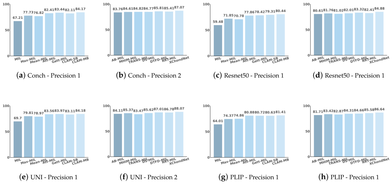
The precision visualizations in Figure 5 further confirm these findings. XChondNet maintains stable and superior accuracy. This stability indicates that the model’s attention aligns with clinically relevant regions. Taken together, these results demonstrate XChondNet’s consistent advantages over existing MIL frameworks, supporting its potential for practical application in pathology diagnosis. To further validate the statistical reliability of the comparative experiments, we conducted paired significance analysis on ACC between XChondNet and two strong MIL baselines, DTFD-MIL and RRT-MIL. These two methods were selected because they achieved the best or near-best performance among the compared MIL-based methods in Table 2. Specifically, the comparison was conducted across four feature extractors, including Conch, ResNet-50, UNI, and PLIP, resulting in eight paired comparisons. As shown in Figure 4, XChondNet consistently outperforms DTFD-MIL and RRT-MIL under different feature extractor settings. The average ACC of the two strong baselines is 85.16%, whereas XChondNet achieves an average ACC of 86.58%, corresponding to an average improvement of 1.42%. The paired significance analysis further confirms that this improvement is statistically significant, with a paired t-test result of and a Wilcoxon signed-rank test result of . These results indicate that the superiority of XChondNet is not only reflected in higher average performance, but is also statistically supported when compared with competitive MIL methods from the literature.
Figure 4.
Paired statistical significance analysis of ACC between XChondNet and two strong MIL baselines, DTFD-MIL and RRT-MIL. The comparison was conducted across four feature extractors, including Conch, ResNet-50, UNI, and PLIP.
Figure 4.
Paired statistical significance analysis of ACC between XChondNet and two strong MIL baselines, DTFD-MIL and RRT-MIL. The comparison was conducted across four feature extractors, including Conch, ResNet-50, UNI, and PLIP.
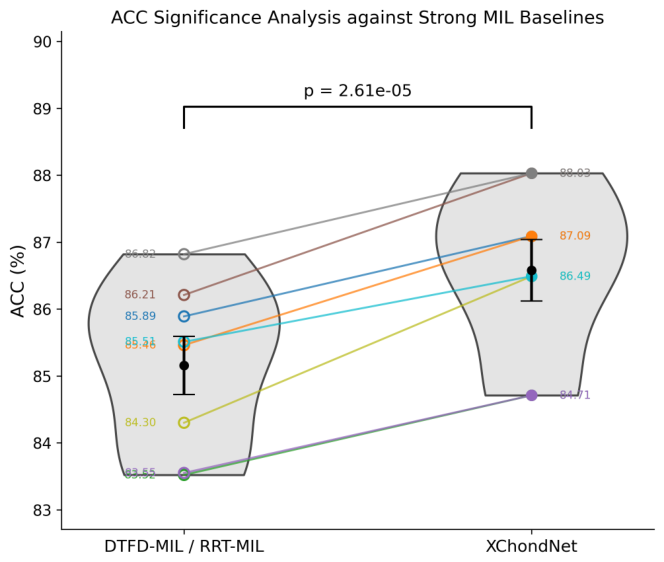
Figure 5.
Visualization of the precision performance in comparative experiments across the Conch, Resnet50, UNI and PLIP feature extractor.
Figure 5.
Visualization of the precision performance in comparative experiments across the Conch, Resnet50, UNI and PLIP feature extractor.
4.5. Why We Choose the Mechanism of Fusing Pathological and Positional Features?
To further validate the contribution of each component, we conducted a set of ablation experiments. Here, w/o denotes “without.” Specifically, w/o position features removes the positional encoding branch and relies solely on pathological features; w/o intra-class attention discards the intra-class attention module; w/o inter-class attention eliminates the inter-class attention mechanism to break structural dependencies across classes; w/o prototype constraint drops the prototype-based regularization loss while keeping the rest unchanged.
For clarity, the following abbreviations are used in the ablation study: w/o pos denotes the removal of position features, i.e., the model relies solely on pathological features; w/o Intra indicates the elimination of the intra-class attention module; w/o Inter refers to the removal of the inter-class attention mechanism, thereby breaking structural dependencies across classes; and w/o Pro represents the exclusion of the prototype-based regularization constraint while keeping other components unchanged.
Table 3 summarizes the ablation study results, while Figure 6 further illustrates the precision evaluation metric across different settings. The complete model achieves the best performance in terms of ACC, AUC, F1, and Recall, confirming the effectiveness of the proposed design. Among the components, w/o pos leads to the most significant degradation, highlighting the critical role of spatial information in pathological representation of Chondrogenic tumors. w/o Intra demonstrates the necessity of modeling local dependencies among instances. In contrast, w/o Inter and w/o Pro causes relatively smaller reductions, but both still contribute to improving global structure modeling.
4.6. Why We Choose the Parallel Classifier Mechanism?
To assess the contribution of the parallel classifier mechanism, we performed an ablation study using features extracted from four different feature extractors. The full model was compared with variants w/o PC (without the parallel classifier), where each feature set was processed by a single classifier instead of parallel classifiers, while all other components remained unchanged. In the results table, ✓ indicates the presence of the parallel classifier mechanism, and ✗ indicates its absence.
The ablation results across the four feature extractors consistently demonstrate the effectiveness of the parallel classifier mechanism. As shown in Table 4 and Figure 7, removing this mechanism leads to a degradation across all evaluation metrics. In contrast, the full model with ✓ achieves consistently higher precision, recall, and AUC, indicating that parallel classifiers can better exploit the complementary information from multiple feature representations. These findings confirm that the parallel classifier mechanism enhances the discriminative capability of the proposed framework.
To further validate the reliability of the ablation results, we conducted paired statistical significance analysis on the ablation experiments. For the component ablation study, the full XChondNet was compared with its ablated variants under the same feature extractor settings, including the variants without positional features, intra-class attention, inter-class attention, and prototype constraint. As shown in Figure 8, XChondNet consistently achieved higher ACC values than the corresponding ablated variants across different feature extractors, and the improvement was statistically significant with a paired test result of . This indicates that the proposed positional modeling, intra-class attention, inter-class attention, and prototype constraint jointly contribute to more effective pathological feature representation.
For the parallel classifier ablation, we further compared XChondNet with and without the parallel classifier mechanism. The paired analysis across different feature extractors showed that introducing the parallel classifier led to consistent performance gains, with a statistically significant improvement of . This result demonstrates that the parallel classifier can enhance category-specific discrimination, which is particularly beneficial for chondrogenic tumor diagnosis with imbalanced subtype distributions.
4.7. Temporal Validation and Domain-Shift Analysis
To further evaluate the generalization ability of XChondNet and reduce the potential risk of overfitting caused by the limited dataset size, we conducted additional temporal validation and domain-shift robustness analyses. For temporal validation, all patients were split according to the chronological order of sample collection. Cases collected from 2017 to 2022 were used for training and validation, while cases collected from 2023 to 2024 were held out as an independent temporal test set. This setting is more challenging than random cross-validation because the test samples are temporally separated from the training data, thereby providing a more realistic evaluation of model robustness over time. Importantly, the temporal split was performed at the patient level to avoid information leakage.
As shown in Table 5, XChondNet maintained stable diagnostic performance on the temporally independent test set. Under the same UNI feature extractor and temporal split setting, XChondNet achieved an ACC of 86.82%, AUC of 97.23%, F1 score of 86.87%, and Recall of 86.76%. Compared with two strong MIL baselines, XChondNet outperformed DTFD-MIL by 1.35% in ACC and RRT-MIL by 0.89% in ACC. Similar improvements were also observed in F1 score and Recall. These results suggest that XChondNet can maintain relatively robust diagnostic performance on chronologically separated cases, indicating its potential temporal generalization ability.
In addition, we performed a domain-shift robustness analysis to evaluate whether XChondNet remains stable under different feature-domain settings. Specifically, different pathological feature extractors, including Conch, ResNet-50, UNI, and PLIP, were regarded as different feature-domain settings because they generate different representation spaces. To make the analysis more convincing, XChondNet was compared with two strong MIL baselines, DTFD-MIL and RRT-MIL, under the same feature-domain settings.
As shown in Table 6, XChondNet consistently achieved higher ACC than DTFD-MIL and RRT-MIL across all four feature-domain settings. Specifically, XChondNet obtained a mean ACC of 86.58%, outperforming DTFD-MIL and RRT-MIL, which achieved mean ACC values of 84.98% and 85.34%, respectively. The average ACC improvements over DTFD-MIL and RRT-MIL were 1.60% and 1.24%, respectively. These results indicate that the proposed framework is not overly dependent on a single feature extractor and can maintain robust diagnostic performance under different feature-domain conditions.
4.8. Statistical Analysis and Reliability Evaluation
To further support the reliability of the final comparison, we added a comprehensive statistical analysis, including confidence interval estimation, paired significance testing, bootstrap analysis, ROC confidence-band visualization, and per-class performance evaluation. Since DTFD-MIL and RRT-MIL achieved strong performance among the compared MIL methods, they were selected as representative baselines for comparison with XChondNet.
The confidence interval results in Table 7 show that XChondNet achieved the highest ACC, F1-score, and Recall among the compared methods. Although RRT-MIL obtained a slightly higher AUC, XChondNet showed better overall diagnostic performance with stable confidence intervals, supporting the reliability of the final comparison.
We further performed paired statistical significance tests to evaluate whether the ACC improvements of XChondNet over strong MIL baselines were statistically reliable. Specifically, Conch, ResNet-50, UNI, and PLIP were regarded as four paired feature-domain settings. XChondNet was compared with DTFD-MIL and RRT-MIL under the same feature extractor settings.
The significance analysis in Table 8 shows that XChondNet achieved consistent ACC improvements over DTFD-MIL and RRT-MIL across different feature-domain settings. Compared with DTFD-MIL and RRT-MIL, XChondNet improved the mean ACC by 1.60% and 1.25%, respectively. The paired t-test showed statistically significant improvements for both comparisons. When the two strong baselines were jointly considered, XChondNet achieved an average ACC improvement of 1.42%, with significant results in both the paired t-test () and the Wilcoxon signed-rank test (). These results indicate that the marginal ACC gains of XChondNet are statistically supported across different feature-domain settings.
To further estimate the uncertainty of the final performance, we performed bootstrap analysis for XChondNet under the UNI feature extractor. The test samples were repeatedly resampled with replacement, and the evaluation metrics were recalculated for each bootstrap sample. The 2.5th and 97.5th percentiles of the bootstrap distribution were used as the 95% confidence interval.
Table 9 shows that XChondNet achieved stable bootstrap confidence intervals across the main evaluation metrics. The ACC, F1-score, and Recall confidence intervals were centered around the observed values, while the AUC confidence interval remained at a high level. These results indicate that the final performance estimation of XChondNet is stable under bootstrap resampling.
In addition, we generated a bootstrap-based macro-average ROC confidence band to visualize the stability of the ROC curve under resampling. Figure 9 shows the ROC curve remained close to the upper-left region, and the confidence band was relatively narrow, indicating stable discrimination performance of XChondNet under bootstrap resampling.
We further conducted a per-class performance analysis to evaluate the diagnostic ability of XChondNet for each subtype of chondrogenic tumors. Precision, Recall, F1-score, and AUC were calculated for each class under the UNI feature extractor.

Table 10.
Per-class performance of XChondNet under the UNI feature extractor.
| Class | Precision(%) | Recall(%) | F1-score(%) | AUC(%) |
|---|---|---|---|---|
| OC | 89.95 | 88.70 | 89.32 | 98.21 |
| ED | 87.40 | 88.60 | 88.00 | 97.36 |
| CF | 87.90 | 87.24 | 87.57 | 97.48 |
| SE | 86.55 | 88.87 | 87.69 | 96.62 |
| CB | 90.20 | 89.10 | 89.65 | 98.07 |
| CD | 86.77 | 86.57 | 86.67 | 96.72 |
4.9. Interpreting Model Predictions through Attention Heatmaps
To intuitively explain the relative importance assigned by XChondNet to different tissue regions, we first calculated the non-normalized attention scores of all extracted patches in each slide. These scores were then converted into percentile scores and normalized to the range of 0 to 1. Next, the normalized attention scores were mapped to RGB colors using a diverging color map, where high-attention regions are represented in red and low-attention regions are represented in blue. Finally, the generated heatmap was superimposed on the original WSI with a transparency of 0.5, allowing the model-highlighted regions and the underlying morphological structures of the H&E-stained slide to be visualized simultaneously.
As shown in Figure 10, the heatmaps provide intuitive evidence that XChondNet can focus on diagnostically meaningful regions. The images in columns 1, 4, and 5 show heatmap visualizations of osteochondroma. Taking the first column as an example, the tumor presents a typical three-layer spatial structure, including the fibrous membrane, cartilage layer, and bone layer. The second column shows chondromyxoid fibroma, which is usually lobulated with dense perilobular cells and relatively low cellular density in the center. The third column shows subungual exostosis, which has certain histological similarity to osteochondroma and also presents a layered spatial structure, gradually transitioning from the peripheral fibrous layer composed of spindle cells to the germinative fibroblast layer, cartilage layer, and cartilage osteogenic layer. The high-attention regions of XChondNet showed clear spatial correspondence with the pathologist-annotated lesion regions, suggesting that the model can perceive important spatial structural information in chondrogenic tumors.
To further provide quantitative evidence beyond visual interpretation, we conducted an IoU-based overlap analysis between the model-generated heatmaps and pathologist-annotated ROIs. The heatmaps were normalized and binarized to obtain model-highlighted high-attention regions, while the pathologist-annotated ROIs were used as expert reference regions. The IoU values were used to evaluate the spatial consistency between model attention and expert annotation.
As shown in Figure 11, the model-highlighted regions showed substantial overlap with pathologist-annotated ROIs, with IoU values of 0.81 and 0.83 in the representative cases. These results indicate that the heatmaps generated by XChondNet are not only visually interpretable, but also quantitatively consistent with expert-defined diagnostic regions.
4.10. Computational Complexity and Hyperparameter Settings
To further evaluate the practical feasibility and reproducibility of XChondNet, we added computational complexity analysis and summarized the main hyperparameters used in the experiments. The computational cost was evaluated in terms of trainable parameters, inference time, and peak GPU memory usage. All measurements were conducted on an NVIDIA RTX 3090 GPU under the same experimental environment.
As shown in Table 11, XChondNet maintains acceptable computational cost during WSI-level inference. The reported inference time and GPU memory usage provide a practical reference for evaluating the deployment feasibility of the proposed method in computational pathology scenarios.
As shown in Table 12, the key experimental settings and training hyperparameters were explicitly reported to improve the reproducibility of XChondNet. These settings were kept consistent across different feature extractors and comparative experiments.
5. Conclusions
In this study, we successfully developed and validated the XChondNet model, designed for chondrogenic tumors diagnosis. By the mechanism for fusing pathological and positional features and the parallel classifier mechanism, the XChondNet model significantly improves the accuracy and reliability of chondrogenic tumors diagnosis. Experimental results show that the XChondNet model is effective on chondrogenic tumors datasets, providing a new approach for chondrogenic tumors auxiliary diagnosis. However, we recognize limitations such as differences in staining styles and limited samples. To overcome these, we plan to incorporate multimodal technology in future research to better explore spatial feature representation and enhance the model’s diagnostic efficiency. Concurrently, we aim to combine generation technology to mitigate sample insufficiency and further boost model performance. Integrating imaging and pathological slice generation technology can yield more information from limited patient samples, generate additional samples, and refine auxiliary diagnosis accuracy. In summary, the XChondNet model introduces a new solution to computational pathology. Despite existing limitations, we anticipate future enhancements and applications. We hope continuous technological progress and in-depth research will enable the XChondNet model to play an increasingly important role in chondrogenic tumors and other clinicopathological diagnoses.
Author Contributions
Conceptualization, S.X. and G.L.; methodology, S.X., Y.X. and G.L.; software, Y.X.; validation, Y.X., A.L. and J.Y.; formal analysis, Y.X. and J.Y.; investigation, Y.X. and A.L.; resources, A.L. and G.L.; data curation, Y.X. and A.L.; writing—original draft preparation, Y.X.; writing—review and editing, S.X., G.L. and J.Y.; visualization, Y.X.; supervision, S.X. and G.L.; project administration, G.L.; funding acquisition, S.X. and G.L. All authors have read and agreed to the published version of the manuscript.
Funding
This work was supported by the National Natural Science Foundation of China under Grant 62271345 and 62306211.
Institutional Review Board Statement
The study protocol was reviewed and approved by the Ethics Committee of Tianjin Hospital, Tianjin, China.
Data Availability Statement
The data are not publicly available due to privacy and ethical restrictions.
Conflicts of Interest
The authors declare no conflicts of interest.
References
- Gaumer, G. R.; Weinberg, D. S.; Collier, C. D.; Getty, P. J.; Liu, R. W. An osteological study on the prevalence of osteochondromas. Iowa Orthop. J. 2017, 37, 147. [Google Scholar] [PubMed]
- Campanella, G.; Hanna, M. G.; Geneslaw, L.; Miraflor, A.; Werneck Krauss Silva, V.; Busam, K. J.; Brogi, E.; Reuter, V. E.; Klimstra, D. S.; Fuchs, T. J. Clinical-grade computational pathology using weakly supervised deep learning on whole slide images. Nat. Med. 2019, 25(8), 1301–1309. [Google Scholar] [CrossRef] [PubMed]
- Lu, M. Y.; Williamson, D. F.K.; Chen, T. Y.; Chen, R. J.; Barbieri, M.; Mahmood, F. Data-efficient and weakly supervised computational pathology on whole-slide images. Nat. Biomed. Eng. 2021, 5(6), 555–570. [Google Scholar] [CrossRef] [PubMed]
- Zheng, Y.; Li, J.; Shi, J.; Xie, F.; Huai, J.; Cao, M.; Jiang, Z. Kernel attention transformer for histopathology whole slide image analysis and assistant cancer diagnosis. IEEE Trans. Med. Imaging 2023, 42(9), 2726–2739. [Google Scholar] [CrossRef] [PubMed]
- Raju, A.; Yao, J.; Haq, M. M.; Jonnagaddala, J.; Huang, J. Graph attention multi-instance learning for accurate colorectal cancer staging. Medical Image Computing and Computer Assisted Intervention–MICCAI 2020: 23rd International Conference, Lima, Peru, October 4–8, 2020; Proceedings, Part V 23 2020, pp. 529–539. [Google Scholar]
- Xu, J.; Lu, H.; Li, H.; Yan, C.; Wang, X.; Zang, M.; de Rooij, D. G.; Madabhushi, A.; Xu, E. Y. Computerized spermatogenesis staging (CSS) of mouse testis sections via quantitative histomorphological analysis. Med. Image Anal. 2021, 70, 101835. [Google Scholar] [CrossRef] [PubMed]
- Bulten, W.; Kartasalo, K.; Chen, P. C.; Ström, P.; Pinckaers, H.; Nagpal, K.; Cai, Y.; Steiner, D. F.; Van Boven, H.; Vink, R.; et al. Artificial intelligence for diagnosis and Gleason grading of prostate cancer: the PANDA challenge. Nat. Med. 2022, 28(1), 154–163. [Google Scholar] [CrossRef] [PubMed]
- Fu, Y.; Jung, A. W.; Torne, R. V.; Gonzalez, S.; Vöhringer, H.; Shmatko, A.; Yates, L. R.; Jimenez-Linan, M.; Moore, L.; Gerstung, M. Pan-cancer computational histopathology reveals mutations, tumor composition and prognosis. Nat. Cancer 2020, 1(8), 800–810. [Google Scholar] [CrossRef] [PubMed]
- Chen, R. J.; Lu, M. Y.; Wang, J.; Williamson, D. F.K.; Rodig, S. J.; Lindeman, N. I.; Mahmood, F. Pathomic fusion: an integrated framework for fusing histopathology and genomic features for cancer diagnosis and prognosis. IEEE Trans. Med. Imaging 2020, 41(4), 757–770. [Google Scholar]
- Chen, R. J.; Lu, M. Y.; Williamson, D. F.K.; Chen, T. Y.; Lipkova, J.; Noor, Z.; Shaban, M.; Shady, M.; Williams, M.; Joo, B.; et al. Pan-cancer integrative histology-genomic analysis via multimodal deep learning. Cancer Cell 2022, 40(8), 865–878. [Google Scholar] [CrossRef] [PubMed]
- Coudray, N.; Ocampo, P. S.; Sakellaropoulos, T.; Narula, N.; Snuderl, M.; Fenyö, D.; Moreira, A. L.; Razavian, N.; Tsirigos, A. Classification and mutation prediction from non–small cell lung cancer histopathology images using deep learning. Nat. Med. 2018, 24(10), 1559–1567. [Google Scholar] [CrossRef] [PubMed]
- Yamashita, R.; Long, J.; Longacre, T.; Peng, L.; Berry, G.; Martin, B.; Higgins, J.; Rubin, D. L.; Shen, J. Deep learning model for the prediction of microsatellite instability in colorectal cancer: a diagnostic study. Lancet Oncol. 2021, 22(1), 132–141. [Google Scholar] [CrossRef] [PubMed]
- Yan, R.; Shen, Y.; Zhang, X.; Xu, P.; Wang, J.; Li, J.; Ren, F.; Ye, D.; Zhou, S. K. Histopathological bladder cancer gene mutation prediction with hierarchical deep multiple-instance learning. Med. Image Anal. 2023, 87, 102824. [Google Scholar] [CrossRef] [PubMed]
- Lan, G.; Xiao, S.; Yang, J.; Wen, J.; Xi, M. Generative AI-based data completeness augmentation algorithm for data-driven smart healthcare. IEEE J. Biomed. Health Inform. 2023. [Google Scholar] [CrossRef] [PubMed]
- Lan, G.; Xiao, S.; Yang, J.; Wen, J. Generative model perception rectification algorithm for trade-off between diversity and quality. In Proceedings of the AAAI conference on artificial intelligence, 2024; pp. 13328–13336. [Google Scholar]
- Lan, G.; Xiao, S.; Yang, J.; Wen, J.; Lu, W.; Gao, X. Active learning inspired method in generative models. Expert Syst. With Appl. 2024, 249, 123582. [Google Scholar] [CrossRef]
- Jesus-Garcia, R.; Osawa, A.; Filippi, R. Z.; Viola, D. C. M.; Korukian, M.; de Carvalho Campos Neto, G.; Wagner, J. Is PET–CT an accurate method for the differential diagnosis between chondroma and chondrosarcoma? Springerplus 2016, 5, 1–10. [Google Scholar] [CrossRef] [PubMed]
- Wang, X.L.; De Beuckeleer, L.H.; De Schepper, A.M.A.; Van Marck, E. Low-grade chondrosarcoma vs enchondroma: challenges in diagnosis and management. Eur. Radiol. 2001, 11, 1054–1057. [Google Scholar] [CrossRef] [PubMed]
- Bansal, M.; Goldman, A. B.; DiCarlo, E. F.; McCormack, R. Soft tissue chondromas: diagnosis and differential diagnosis. Skelet. Radiol. 1993, 22, 309–315. [Google Scholar] [CrossRef] [PubMed]
- Cates, J. M.; Rosenberg, A. E.; O’Connell, J. X.; Nielsen, G. P. Chondroblastoma-like chondroma of soft tissue: an underrecognized variant and its differential diagnosis. Am. J. Surg. Pathol. 2001, 25(5), 661–666. [Google Scholar] [PubMed]
- Schajowicz, F.; Gallardo, H. Chondromyxoid fibroma (fibromyxoid chondroma) of bone: a clinico-pathological study of thirty-two cases. J. Bone Jt. Surg. Br. 1971, 53(2), 198–216. [Google Scholar]
- Bejnordi, B. E.; Litjens, G.; Timofeeva, N.; Otte-Höller, I.; Homeyer, A.; Karssemeijer, N.; Van Der Laak, J. A.W.M. Stain specific standardization of whole-slide histopathological images. IEEE Trans. Med. Imaging 2015, 35(2), 404–415. [Google Scholar] [CrossRef] [PubMed]
- Lucas, M.; Jansen, I.; Savci-Heijink, C. D.; Meijer, S. L.; de Boer, O. J.; van Leeuwen, T. G.; de Bruin, D. M.; Marquering, H. A. Deep learning for automatic Gleason pattern classification for grade group determination of prostate biopsies. Virchows Arch. 2019, 475, 77–83. [Google Scholar] [CrossRef] [PubMed]
- Raees, P.C. M.; Thomas, V. Automated detection of Alzheimer’s Disease using Deep Learning in MRI. Journal of Physics: Conference Series, 2021; p. 012024. [Google Scholar]
- Wang, G.; Li, W.; Ourselin, S.; Vercauteren, T. Automatic brain tumor segmentation using cascaded anisotropic convolutional neural networks. Brainlesion: Glioma, Multiple Sclerosis, Stroke and Traumatic Brain Injuries: Third International Workshop, BrainLes 2017, Held in Conjunction with MICCAI 2017 Revised Selected Papers 3 2018. 2017, 178–190. [Google Scholar] [CrossRef]
- Zhang, R.; Zheng, Y.; Mak, T. W. C.; Yu, R.; Wong, S. H.; Lau, J. Y.W.; Poon, C. C.Y. Automatic detection and classification of colorectal polyps by transferring low-level CNN features from nonmedical domain. IEEE J. Biomed. Health Inform. 2016, 21(1), 41–47. [Google Scholar] [CrossRef] [PubMed]
- De Matos, J.; Britto, A. d. S.; Oliveira, L. E.S.; Koerich, A. L. Double transfer learning for breast cancer histopathologic image classification. 2019 international joint conference on neural networks (IJCNN), 2019; pp. 1–8. [Google Scholar]
- Saxena, S.; Shukla, S.; Gyanchandani, M. Pre-trained convolutional neural networks as feature extractors for diagnosis of breast cancer using histopathology. Int. J. Imaging Syst. Technol. 2020, 30(3), 577–591. [Google Scholar] [CrossRef]
- Nazeri, K.; Aminpour, A.; Ebrahimi, M. Two-stage convolutional neural network for breast cancer histology image classification. Image Analysis and Recognition: 15th International Conference, ICIAR 2018 Proceedings 15 2018, Póvoa de Varzim, Portugal, June 27–29, 2018; pp. 717–726. [Google Scholar]
- Carbonneau, M.; Cheplygina, V.; Granger, E.; Gagnon, G. Multiple instance learning: A survey of problem characteristics and applications. Pattern Recognit. 2018, 77, 329–353. [Google Scholar] [CrossRef]
- Ilse, M.; Tomczak, J.; Welling, M. Attention-based deep multiple instance learning. International conference on machine learning, 2018; pp. 2127–2136. [Google Scholar]
- Li, B.; Li, Y.; Eliceiri, K. W. Dual-stream multiple instance learning network for whole slide image classification with self-supervised contrastive learning. In Proceedings of the IEEE/CVF conference on computer vision and pattern recognition, 2021; pp. 14318–14328. [Google Scholar]
- Shao, Z.; Bian, H.; Chen, Y.; Wang, Y.; Zhang, J.; Ji, X.; et al. Transmil: Transformer based correlated multiple instance learning for whole slide image classification. Adv. Neural Inf. Process. Syst. 2021, 34, 2136–2147. [Google Scholar]
- Vaswani, A.; Shazeer, N.; Parmar, N.; Uszkoreit, J.; Jones, L.; Gomez, A. N.; Kaiser; Polosukhin, I. Attention is all you need. Adv. Neural Inf. Process. Syst. 2017, 30. [Google Scholar]
- Tang, W.; Zhou, F.; Huang, S.; Zhu, X.; Zhang, Y.; Liu, B. Feature re-embedding: Towards foundation model-level performance in computational pathology. In Proceedings of the IEEE/CVF Conference on Computer Vision and Pattern Recognition, 2024; pp. 11343–11352. [Google Scholar]
- Xie, Y.; Liu, Z.; Zhao, J.; Ma, J. PHIM-MIL: Multiple instance learning with prototype similarity-guided feature fusion and hard instance mining for whole slide image classification. Inf. Fusion 2025, 117, 102847. [Google Scholar] [CrossRef]
- Tang, W.; Huang, S.; Zhang, X.; Zhou, F.; Zhang, Y.; Liu, B. Multiple instance learning framework with masked hard instance mining for whole slide image classification. In Proceedings of the IEEE/CVF International Conference on Computer Vision, 2023; pp. 4078–4087. [Google Scholar]
- Lan, G.; Xiao, S.; Wen, J.; Yang, J.; Lu, W.; Li, B.; Meng, Q.; Gao, X. A deep neural network optimization framework based on optimal transport bridge feature selection and sparse representation. IEEE Trans. Neural Netw. Learn. Syst. 2026, 1–14. [Google Scholar] [CrossRef] [PubMed]
- Otsu, N.; et al. A threshold selection method from gray-level histograms. Automatica 1975, 11(285-296), 23–27. [Google Scholar]
- Jin, K.; Zhang, Z.; Lan, G.; Xiao, S.; Yang, J. NTFold: Structure-Sensing Nucleotide Attention Learning for RNA Secondary Structure Prediction. Sensors 2026, 26(2), 688. [Google Scholar] [CrossRef] [PubMed]
Figure 1.
The case 1 and case 2 are osteochondromas, which are histologically characterized by a typical three-layered spatial structure, fibrous membrane, cartilage and bone. The case 3 and case 4 are subungual exostoses with histologic features ranging from the peripheral fibrous layer of spindle cells to the germinal active fibroblast layer and then to the cartilage and cartilage osteogenic layer.
Figure 1.
The case 1 and case 2 are osteochondromas, which are histologically characterized by a typical three-layered spatial structure, fibrous membrane, cartilage and bone. The case 3 and case 4 are subungual exostoses with histologic features ranging from the peripheral fibrous layer of spindle cells to the germinal active fibroblast layer and then to the cartilage and cartilage osteogenic layer.
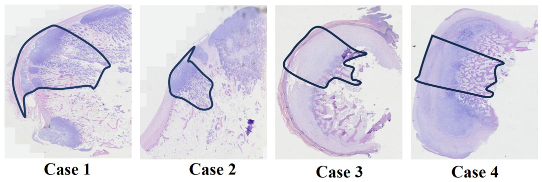
Figure 2.
Technical overview of the proposed XChondNet framework for chondrogenic tumor classification. The framework follows a pathology-driven design: tissue regions are first segmented from WSIs, patch-level pathological features and spatial positional features are then extracted and fused to model both local morphology and spatial tissue organization, and the multi-scale feature enhancement network further strengthens discriminative representations through attention modeling, prototype constraints, and contrastive learning. Finally, parallel classifiers are used to improve category-specific discrimination under imbalanced chondrogenic tumor data.
Figure 2.
Technical overview of the proposed XChondNet framework for chondrogenic tumor classification. The framework follows a pathology-driven design: tissue regions are first segmented from WSIs, patch-level pathological features and spatial positional features are then extracted and fused to model both local morphology and spatial tissue organization, and the multi-scale feature enhancement network further strengthens discriminative representations through attention modeling, prototype constraints, and contrastive learning. Finally, parallel classifiers are used to improve category-specific discrimination under imbalanced chondrogenic tumor data.
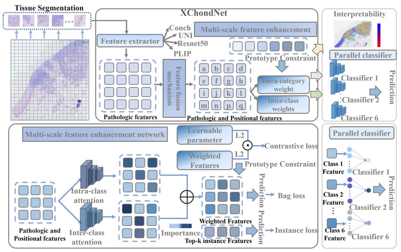
Figure 3.
Representative histopathological images of six categories of chondrogenic tumors tumors: (a) osteochondroma, (b) enchondroma, (c) chondromyxoid fibroma, (d) subungual exostosis, (e) chondroblastoma, and (f) chondrosarcoma.
Figure 3.
Representative histopathological images of six categories of chondrogenic tumors tumors: (a) osteochondroma, (b) enchondroma, (c) chondromyxoid fibroma, (d) subungual exostosis, (e) chondroblastoma, and (f) chondrosarcoma.
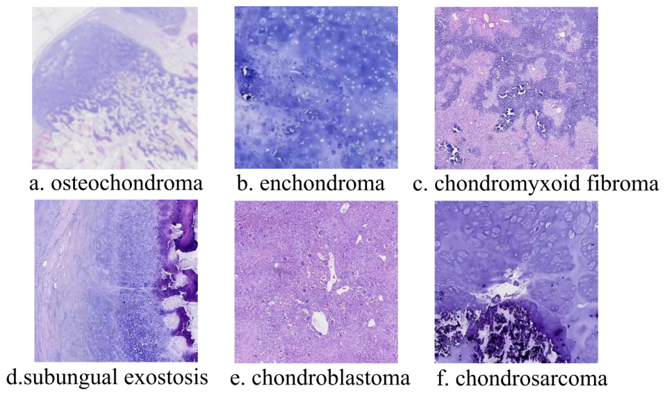
Figure 6.
Visualization of the precision performance in ablation experiments across the Conch, Resnet50, UNI and PLIP feature extractor.
Figure 6.
Visualization of the precision performance in ablation experiments across the Conch, Resnet50, UNI and PLIP feature extractor.
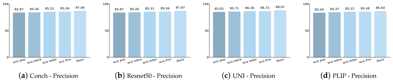
Figure 7.
Ablation experiment precision of the parallel classifier mechanism.
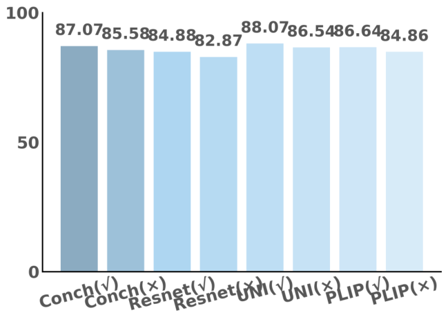
Figure 8.
Paired statistical significance analysis of the ablation experiments on ACC. The full XChondNet shows significant improvements over the ablated variants in the component ablation study, and the parallel classifier mechanism also brings statistically significant performance gains across different feature extractors.
Figure 8.
Paired statistical significance analysis of the ablation experiments on ACC. The full XChondNet shows significant improvements over the ablated variants in the component ablation study, and the parallel classifier mechanism also brings statistically significant performance gains across different feature extractors.
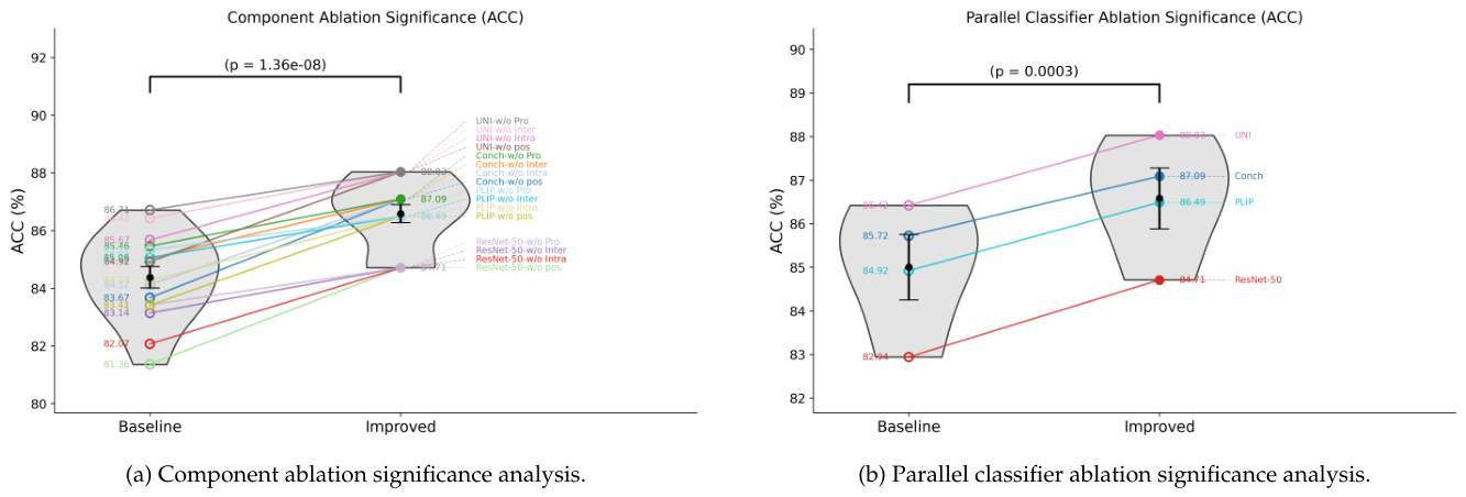
Figure 9.
Bootstrap-based macro-average ROC confidence band of XChondNet under the UNI feature extractor. The solid curve represents the mean macro-average ROC curve, and the shaded region indicates the 95% confidence band estimated by bootstrap resampling.
Figure 9.
Bootstrap-based macro-average ROC confidence band of XChondNet under the UNI feature extractor. The solid curve represents the mean macro-average ROC curve, and the shaded region indicates the 95% confidence band estimated by bootstrap resampling.
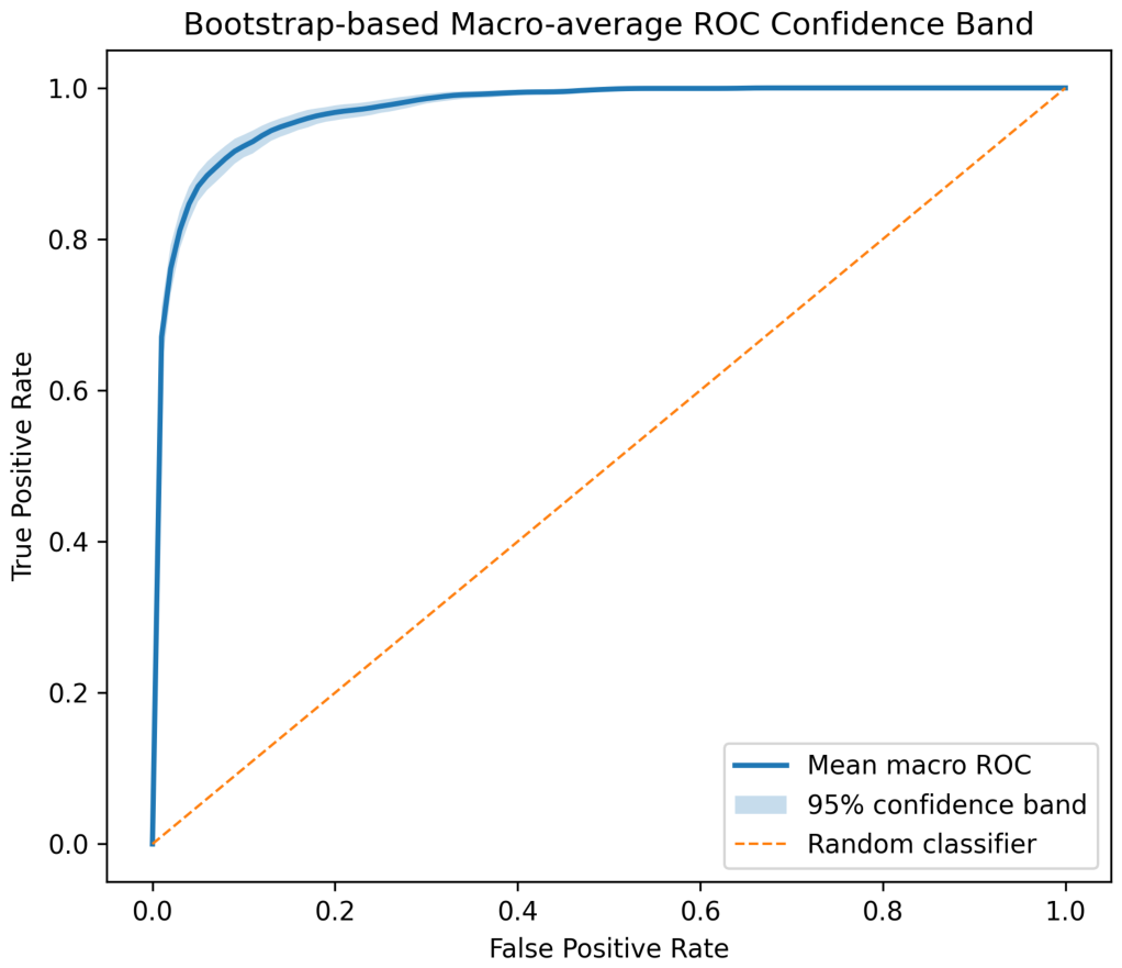
Figure 10.
Heatmap visualization and clinical consistency analysis of XChondNet on representative chondrogenic tumor cases. The top row shows the original pathological images, the middle row shows the pathologist-annotated lesion regions, and the bottom row shows the heatmap-based recognition results generated by XChondNet. This visualization is used to assess whether the model-highlighted regions are spatially consistent with clinically meaningful lesion areas identified by the pathologist.
Figure 10.
Heatmap visualization and clinical consistency analysis of XChondNet on representative chondrogenic tumor cases. The top row shows the original pathological images, the middle row shows the pathologist-annotated lesion regions, and the bottom row shows the heatmap-based recognition results generated by XChondNet. This visualization is used to assess whether the model-highlighted regions are spatially consistent with clinically meaningful lesion areas identified by the pathologist.
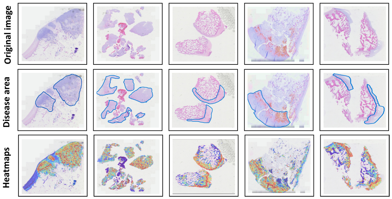
Figure 11.
Representative examples of IoU-based consistency analysis between XChondNet heatmaps and pathologist-annotated ROIs. The blue contours indicate the pathologist-annotated ROIs, and the heatmaps represent model-highlighted discriminative regions. The IoU values are 0.81 and 0.83, respectively.
Figure 11.
Representative examples of IoU-based consistency analysis between XChondNet heatmaps and pathologist-annotated ROIs. The blue contours indicate the pathologist-annotated ROIs, and the heatmaps represent model-highlighted discriminative regions. The IoU values are 0.81 and 0.83, respectively.
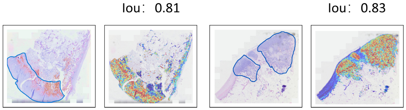
Table 1.
Pathological data type distribution and data division.
| Category | Data type | Data division | ||||
|---|---|---|---|---|---|---|
| WSI | ROI | Train | Valid | Test | ||
| OC | 31 | 295 | 235 | 30 | 30 | |
| ED | 17 | 159 | 117 | 17 | 25 | |
| CF | 39 | 507 | 412 | 61 | 34 | |
| SE | 15 | 107 | 76 | 17 | 14 | |
| CB | 15 | 216 | 168 | 21 | 27 | |
| CD | 22 | 188 | 139 | 16 | 33 | |
Table 2.
Comparative performance of different MIL-based methods on Conch, Resnet-50, UNI, and PLIP feature extractors. The best results are highlighted in bold. Evaluation metrics include ACC, AUC, F1 score, and Recall.
Table 2.
Comparative performance of different MIL-based methods on Conch, Resnet-50, UNI, and PLIP feature extractors. The best results are highlighted in bold. Evaluation metrics include ACC, AUC, F1 score, and Recall.
| Method | Conch | Resnet-50 | ||||||
|---|---|---|---|---|---|---|---|---|
| ACC(%) | AUC(%) | F1(%) | Recall(%) | ACC(%) | AUC(%) | F1(%) | Recall(%) | |
| MIL | 68.67±2.29 | 85.52±0.98 | 68.86±2.27 | 68.67±2.29 | 58.17±2.38 | 77.23±1.23 | 58.86±2.57 | 58.79±2.47 |
| Max-MIL | 77.39±2.13 | 92.12±1.11 | 77.86±2.12 | 77.47±2.11 | 71.27±2.46 | 88.39±1.44 | 71.83±2.19 | 71.82±2.13 |
| Mean-MIL | 76.89±3.07 | 93.67±1.80 | 76.48±2.98 | 76.26±3.03 | 70.47±2.47 | 87.98±1.83 | 70.67±2.31 | 70.66±2.42 |
| Att-MIL | 82.37±2.49 | 96.62±0.81 | 82.48±2.31 | 82.44±2.46 | 77.94±2.58 | 94.62±1.28 | 77.91±2.49 | 77.89±2.51 |
| Gatt-MIL | 83.14±1.94 | 97.02±1.12 | 83.46±1.89 | 83.48±1.91 | 79.18±2.04 | 95.06±1.23 | 78.48±2.18 | 78.66±2.24 |
| CLAM-SB | 82.07±2.34 | 96.04±0.96 | 82.24±2.14 | 82.03±2.38 | 79.66±2.67 | 94.51±0.61 | 79.46±2.81 | 79.83±2.88 |
| CLAM-MB | 83.83±2.23 | 96.83±0.94 | 84.01±2.02 | 83.77±2.13 | 80.25±2.20 | 94.18±0.65 | 80.29±2.10 | 80.22±2.14 |
| AB-MIL | 83.77±1.88 | 96.23±0.77 | 83.94±1.91 | 83.77±1.91 | 80.75±1.91 | 95.14±1.12 | 80.56±2.01 | 80.46±1.97 |
| MHIM-MIL | 84.65±1.86 | 97.09±0.20 | 84.80±1.47 | 84.65±1.86 | 81.23±1.97 | 95.22±1.37 | 81.86±1.82 | 81.33±1.91 |
| TRANS-MIL | 84.92±1.74 | 96.64±0.64 | 84.99±1.61 | 84.92±1.74 | 81.09±1.74 | 94.53±1.13 | 81.03±1.73 | 81.03±1.76 |
| DS-MIL | 84.78±1.40 | 97.23±0.20 | 84.94±1.30 | 84.78±1.40 | 82.04±1.12 | 95.88±0.89 | 82.00±1.07 | 81.96±1.04 |
| DTFD-MIL | 85.89±1.31 | 96.89±0.56 | 85.86±1.37 | 85.87±1.32 | 83.52±1.10 | 95.10±1.71 | 83.22±1.38 | 83.35±1.41 |
| RRT-MIL | 85.46±1.21 | 97.67±0.53 | 85.53±1.61 | 85.46±1.21 | 83.55±1.72 | 95.78±0.76 | 82.47±1.62 | 82.42±1.61 |
| XChondNet | 87.09±1.38 | 97.26±0.51 | 87.14±1.44 | 87.08±1.36 | 84.71±2.16 | 95.96±0.91 | 84.69±2.57 | 84.72±2.59 |
| Method | UNI | PLIP | ||||||
| ACC(%) | AUC(%) | F1(%) | Recall(%) | ACC(%) | AUC(%) | F1(%) | Recall(%) | |
| MIL | 69.21±2.08 | 86.41±1.72 | 69.63±2.21 | 69.67±2.31 | 64.27±2.91 | 82.23±1.64 | 63.76±2.62 | 63.77±2.61 |
| Max-MIL | 79.41±1.83 | 93.25±1.07 | 79.75±1.92 | 79.71±1.94 | 74.37±2.26 | 91.29±1.67 | 74.33±2.17 | 74.32±2.18 |
| Mean-MIL | 78.91±1.73 | 93.37±1.16 | 78.87±1.77 | 78.89±1.76 | 74.71±2.41 | 92.31±1.72 | 74.36±2.04 | 74.38±2.03 |
| Att-MIL | 83.47±2.17 | 96.53±0.97 | 83.46±2.11 | 83.44±2.12 | 80.74±2.46 | 95.27±1.09 | 80.91±2.38 | 80.96±2.41 |
| Gatt-MIL | 83.87±1.97 | 96.31±1.12 | 83.91±1.89 | 83.93±1.92 | 80.89±2.32 | 95.41±0.96 | 80.78±2.41 | 80.77±2.43 |
| CLAM-SB | 83.01±2.43 | 96.49±1.23 | 83.04±2.47 | 83.06±2.48 | 80.46±2.52 | 95.71±0.88 | 80.51±2.53 | 80.53±2.54 |
| CLAM-MB | 84.21±1.78 | 97.02±0.77 | 84.06±1.81 | 84.05±1.83 | 81.27±2.21 | 96.21±0.92 | 81.31±2.23 | 81.26±2.31 |
| AB-MIL | 84.01±1.66 | 96.89±0.87 | 84.07±1.95 | 84.08±1.98 | 81.79±1.98 | 96.41±0.88 | 81.81±1.93 | 81.86±1.89 |
| MHIM-MIL | 85.25±1.67 | 97.16±0.44 | 85.30±1.69 | 85.35±1.66 | 83.31±1.77 | 96.87±1.12 | 83.46±1.81 | 82.43±1.87 |
| TRANS-MIL | 83.82±1.94 | 96.44±1.14 | 83.89±1.97 | 83.87±1.91 | 82.78±1.81 | 95.53±0.87 | 82.83±1.79 | 82.84±1.82 |
| DS-MIL | 85.82±1.39 | 97.01±0.56 | 85.80±1.38 | 85.85±1.41 | 84.27±1.61 | 96.49±1.03 | 84.26±1.59 | 84.23±1.57 |
| DTFD-MIL | 86.21±0.97 | 96.96±0.71 | 86.30±1.03 | 86.34±1.06 | 84.30±1.87 | 96.38±1.11 | 84.36±1.84 | 84.43±1.77 |
| RRT-MIL | 86.82±0.83 | 97.81±0.41 | 86.93±0.74 | 86.88±0.76 | 85.51±1.63 | 96.21±0.67 | 85.53±1.67 | 85.56±1.71 |
| XChondNet | 88.03±0.97 | 97.41±0.84 | 88.14±1.02 | 88.18±1.01 | 86.49±1.94 | 96.35±0.84 | 86.63±1.87 | 86.49±1.91 |
Table 3.
Ablation results of the proposed model under different feature extractors (Conch, ResNet-50, UNI, and PLIP), evaluated by ACC, AUC, F1, and Recall. The best results are highlighted in bold.
Table 3.
Ablation results of the proposed model under different feature extractors (Conch, ResNet-50, UNI, and PLIP), evaluated by ACC, AUC, F1, and Recall. The best results are highlighted in bold.
| Method | Conch | Resnet-50 | ||||||
|---|---|---|---|---|---|---|---|---|
| ACC(%) | AUC(%) | F1(%) | Recall(%) | ACC(%) | AUC(%) | F1(%) | Recall(%) | |
| w/o pos | 83.67±2.12 | 95.32±0.98 | 83.72±2.21 | 83.61±2.19 | 81.36±2.84 | 94.72±1.12 | 81.41±2.93 | 81.28±2.89 |
| w/o Intra | 84.12±1.96 | 95.64±1.02 | 84.25±2.01 | 84.09±1.94 | 82.07±2.55 | 95.01±1.04 | 82.15±2.61 | 82.03±2.58 |
| w/o Inter | 85.03±1.77 | 96.21±0.89 | 85.11±1.82 | 85.07±1.85 | 83.14±2.33 | 95.32±0.97 | 83.19±2.41 | 83.11±2.39 |
| w/o Pro | 85.46±2.08 | 96.42±0.95 | 85.39±2.12 | 85.44±2.05 | 83.42±2.47 | 95.48±0.95 | 83.39±2.52 | 83.44±2.49 |
| Ours | 87.09±1.38 | 97.26±0.51 | 87.14±1.44 | 87.08±1.36 | 84.71±2.16 | 95.96±0.91 | 84.69±2.57 | 84.72±2.59 |
| Method | UNI | PLIP | ||||||
| ACC(%) | AUC(%) | F1(%) | Recall(%) | ACC(%) | AUC(%) | F1(%) | Recall(%) | |
| w/o pos | 84.92±1.62 | 95.86±1.07 | 85.01±1.71 | 84.97±1.69 | 83.41±2.45 | 94.92±1.03 | 83.56±2.52 | 83.39±2.48 |
| w/o Intra | 85.67±1.48 | 96.12±0.99 | 85.74±1.55 | 85.69±1.53 | 84.27±2.21 | 95.14±0.97 | 84.36±2.28 | 84.25±2.24 |
| w/o Inter | 86.42±1.25 | 96.58±0.91 | 86.49±1.31 | 86.44±1.29 | 85.06±2.08 | 95.63±0.91 | 85.19±2.13 | 85.11±2.12 |
| w/o Pro | 86.71±1.34 | 96.72±0.88 | 86.77±1.39 | 86.73±1.36 | 85.32±2.14 | 95.78±0.89 | 85.41±2.18 | 85.36±2.15 |
| Ours | 88.03±0.97 | 97.41±0.84 | 88.14±1.02 | 88.18±1.01 | 86.49±1.94 | 96.35±0.84 | 86.63±1.87 | 86.49±1.91 |
Table 4.
Ablation results of the proposed model about the parallel classifier mechanism under different feature extractors (Conch, ResNet-50, UNI, and PLIP), evaluated by ACC, AUC, F1, and Recall. The best results are highlighted in bold.
Table 4.
Ablation results of the proposed model about the parallel classifier mechanism under different feature extractors (Conch, ResNet-50, UNI, and PLIP), evaluated by ACC, AUC, F1, and Recall. The best results are highlighted in bold.
| Setting | Performance | |||
|---|---|---|---|---|
| ACC(%) | AUC(%) | F1 score(%) | Recall(%) | |
| Conch(✓) | 87.09±1.38 | 97.26±0.51 | 87.14±1.44 | 87.08±1.36 |
| Conch(✗) | 85.72±1.65 | 95.84±0.73 | 85.61±1.58 | 85.47±1.62 |
| Resnet50(✓) | 84.71±2.16 | 95.96±0.91 | 84.69±2.57 | 84.72±2.59 |
| Resnet50(✗) | 82.94±2.43 | 94.87±1.12 | 82.68±2.71 | 82.73±2.65 |
| UNI(✓) | 88.03±0.97 | 97.41±0.84 | 88.14±1.02 | 88.18±1.01 |
| UNI(✗) | 86.42±1.28 | 96.35±1.07 | 86.51±1.33 | 86.47±1.29 |
| PLIP(✓) | 86.49±1.94 | 96.35±0.84 | 86.63±1.87 | 86.49±1.91 |
| PLIP(✗) | 84.92±2.21 | 95.12±1.03 | 85.01±2.14 | 84.88±2.19 |
Table 5.
Temporal validation results on the chronologically separated test set. Cases collected from 2017 to 2022 were used for training and validation, while cases collected from 2023 to 2024 were held out as an independent temporal test set.
Table 5.
Temporal validation results on the chronologically separated test set. Cases collected from 2017 to 2022 were used for training and validation, while cases collected from 2023 to 2024 were held out as an independent temporal test set.
| Method | Feature Extractor | ACC(%) | AUC(%) | F1(%) | Recall(%) |
|---|---|---|---|---|---|
| DTFD-MIL | UNI | 85.47±0.46 | 95.87±0.82 | 85.42±1.69 | 85.38±1.41 |
| RRT-MIL | UNI | 85.93±0.66 | 97.12±0.75 | 85.90±0.68 | 85.83±0.62 |
| XChondNet | UNI | 86.82±1.01 | 97.23±0.99 | 86.87±1.41 | 86.76±1.38 |
Table 6.
Domain-shift robustness analysis under different feature-domain settings. ACC values are reported across four feature extractors.
Table 6.
Domain-shift robustness analysis under different feature-domain settings. ACC values are reported across four feature extractors.
| Method | Conch | ResNet-50 | UNI | PLIP | Mean ACC |
|---|---|---|---|---|---|
| DTFD-MIL | 85.89 | 83.52 | 86.21 | 84.30 | 84.98 |
| RRT-MIL | 85.46 | 83.55 | 86.82 | 85.51 | 85.34 |
| XChondNet | 87.09 | 84.71 | 88.03 | 86.49 | 86.58 |
Table 7.
Final comparison with 95% confidence intervals under the UNI feature extractor.
| Method | ACC(%) | AUC(%) | F1(%) | Recall(%) |
|---|---|---|---|---|
| DTFD-MIL | 86.21 [85.01, 87.41] | 96.96 [96.08, 97.84] | 86.30 [85.02, 87.58] | 86.34 [85.02, 87.66] |
| RRT-MIL | 86.82 [85.79, 87.85] | 97.81 [97.30, 98.32] | 86.93 [86.01, 87.85] | 86.88 [85.94, 87.82] |
| XChondNet | 88.03 [86.83, 89.23] | 97.41 [96.37, 98.45] | 88.14 [86.87, 89.41] | 88.18 [86.93, 89.43] |
Table 8.
Statistical significance analysis of ACC improvements between XChondNet and strong MIL baselines across four feature-domain settings.
Table 8.
Statistical significance analysis of ACC improvements between XChondNet and strong MIL baselines across four feature-domain settings.
| Comparison | Mean ACC Difference(%) | Paired t-test | Wilcoxon Test | Significance |
|---|---|---|---|---|
| XChondNet vs DTFD-MIL | 1.60 | ** | ||
| XChondNet vs RRT-MIL | 1.25 | ** | ||
| XChondNet vs DTFD-MIL and RRT-MIL | 1.42 | *** |
Table 9.
Bootstrap-based confidence intervals of XChondNet under the UNI feature extractor.
| Metric | Observed Value(%) | Bootstrap 95% CI(%) |
|---|---|---|
| ACC | 88.03 | [85.76, 90.18] |
| AUC | 97.41 | [96.23, 98.47] |
| F1-score | 88.14 | [85.92, 90.37] |
| Recall | 88.18 | [85.69, 90.44] |
Table 11.
Computational complexity analysis of XChondNet.
| Model | Params(M) | Inference Time(s/WSI) | GPU Memory(GB) |
|---|---|---|---|
| XChondNet | 2.61 | 7.94 | 7.92 |
Table 12.
Main hyperparameters used in XChondNet.
| Hyperparameter | Value |
|---|---|
| Magnification | 20× |
| Feature extractors | Conch, ResNet-50, UNI, PLIP |
| Feature dimension | 512 |
| Optimizer | Adam |
| Learning rate | 0.001 |
| Weight decay | |
| Batch size | 1 |
| Validation interval | Every 200 epochs |
| Early stopping | Yes |
| Evaluation protocol | 5-fold cross-validation |
| Train/Validation/Test split | 8:1:1 |
| Number of classes | 6 |
| GPU | NVIDIA RTX 3090 |
Disclaimer/Publisher’s Note: The statements, opinions and data contained in all publications are solely those of the individual author(s) and contributor(s) and not of MDPI and/or the editor(s). MDPI and/or the editor(s) disclaim responsibility for any injury to people or property resulting from any ideas, methods, instructions or products referred to in the content. |
© 2026 by the authors. Licensee MDPI, Basel, Switzerland. This article is an open access article distributed under the terms and conditions of the Creative Commons Attribution (CC BY) license (http://creativecommons.org/licenses/by/4.0/).
Copyright: This open access article is published under a Creative Commons CC BY 4.0 license, which permit the free download, distribution, and reuse, provided that the author and preprint are cited in any reuse.