

Submitted:
24 August 2026
Posted:
25 August 2026
You are already at the latest version
Abstract
Quantum algorithms have been proposed for most computational tasks in trading, but the resulting literature is not a single body of work with a single standard of evidence. This survey partitions it into strands with distinct foundations and assesses each against the strongest available evidence. Pricing and market-risk computation rest on quantum amplitude estimation and carry a proven quadratic advantage in inverse precision; circuit-level resource estimates place the requirement at roughly 8000 logical qubits and a logical clock rate of tens of megahertz, several orders of magnitude beyond demonstrated hardware, with joint estimation of prices and sensitivities the main lever that lowers it. Combinatorial formulations of portfolio selection, multi-period trading trajectories and arbitrage detection map onto quadratic unconstrained binary optimization and have the field’s most mature hardware demonstrations, but an extensive benchmark on 250 real-stock instances finds classical mixed-integer programming and tailored heuristics dominant. Quantum machine learning for return prediction has been substantially dequantized, and a controlled evaluation on cross-sectional equity returns attributes reported advantages to evaluation protocol rather than to the model. A fourth strand exploits entanglement for decision coordination under latency constraints, where the advantage follows from Bell’s theorem rather than a complexity assumption. We identify the classical-quantum interface, superquadratic structure, resource-estimate methodology, nonlocal-game design and adversarial benchmarking as the productive open directions.
Keywords:
quantum algorithms
; quantitative finance
; algorithmic trading
; amplitude estimation
; derivative pricing
; portfolio optimization
; dequantization
; quantum machine learning
; resource estimation
; quantum advantage
1. The Shape of the Field
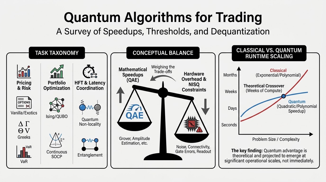
Trading is not one computational problem, and the quantum literature that claims to address it is not one body of work. It is three, with almost disjoint intellectual foundations and radically different evidentiary standards. The first is a pricing and risk literature built on quantum amplitude estimation, where the speedup is proven, the constant factors have been computed to circuit level, and the verdict is a hard resource threshold rather than an open question. The second is a combinatorial optimization literature (portfolio selection, multi-period trading trajectories, arbitrage cycles) where the quantum methods are heuristics with no proven advantage, the hardware demonstrations are the most mature in the field, and the honest benchmarks are unflattering. The third is a machine learning literature applying quantum kernels, variational circuits and generative models to return prediction and hedging, where the theoretical foundations have been actively eroded by dequantization results and the empirical claims are fragile under proper protocol. A fourth strand, small but conceptually distinct, uses entanglement not for speed at all but to coordinate decisions under latency constraints. Table 1 and Figure 1 summarise the resulting landscape. Appendix B documents the construction of that figure, the reported basis for every placement in it, and the arithmetic behind the crossover panel.
For someone entering from classical algorithms, the single most useful reorientation is this: in quantum finance, the interesting questions are almost never “is there an asymptotic speedup?” They are “what is the constant factor, what is the input model, and what does the classical competitor actually cost?” The field’s most valuable papers are the ones that answer those three questions in the same document. Herman et al. [1] is the standard entry point, a survey covering pricing, optimization and machine learning with explicit attention to caveats. Meanwhile Dalzell et al. [2] is the reference work for end-to-end complexity accounting across quantum applications generally, written in a modular form that lets you read the finance sections against the primitives they depend on. Two earlier surveys, Orús, Mugel & Lizaso [3] and Bouland et al. [4], are useful for the historical framing of what the field expected in 2019–2020, which is instructive to compare against what has since been established. Egger et al. [5] covers the same ground from an implementation perspective, and Gómez et al. [6] focuses specifically on derivatives pricing and value-at-risk.
2. Pricing and Risk
2.1. The Core Primitive
The pricing literature rests on a single algorithmic idea. Classical Monte Carlo estimates an expectation to additive error using samples; quantum amplitude estimation, introduced by Brassard et al. [20] as a generalization of Grover [21]’s search, does it with calls to a unitary that prepares the relevant superposition. Montanaro [22] made the general statement for Monte Carlo speedup precise, giving near-quadratic improvements for estimating expectations of bounded random variables and, importantly, quantifying the dependence on the variance rather than assuming boundedness. That quadratic factor is the whole of the advantage, and everything that follows in this section is about whether the overheads consume it.
The translation to finance was made concrete by Rebentrost et al. [23] for European options and generalized by Stamatopoulos et al. [24] to a broad class of payoffs including path-dependent and multi-asset instruments, with the crucial engineering contribution of a piecewise-linear payoff approximation that keeps the quantum arithmetic shallow. Ramos-Calderer et al. [25] developed a related unary-encoding approach that trades qubit count for circuit depth, a sensible trade on near-term hardware, though it forfeits the asymptotic advantage. Extensions to specific instrument classes followed: Kaneko et al. [26] handle local volatility models so that the pricing engine reproduces the observed implied volatility smile rather than a flat Black-Scholes surface, Miyamoto [27] attacks Bermudan options by combining amplitude estimation with Chebyshev interpolation of the continuation value, Alcazar et al. [28] address credit valuation adjustments, and Tang et al. [29] treat collateralized debt obligations.
A separate line replaces sampling with differential equations. An et al. [10] give a quantum multilevel Monte Carlo method for stochastic differential equations that improves the error dependence from to nearly in a setting where naive amplitude estimation struggles, and Alghassi et al. [30] formulate the Feynman-Kac representation variationally. González-Conde et al. [31] solve the pricing PDE directly using quantum linear-systems machinery, and Sakurai et al. [32] apply tensor-train methods to Fourier-based pricing. The latter is quantum-inspired rather than quantum, which makes it a competitor to the quantum proposals rather than an instance of them, and that framing matters for anyone assessing the field.
2.2. The Resource Threshold
The paper that changed the terms of debate is Chakrabarti et al. [7], which gave the first complete resource estimate for useful quantum derivative pricing. Their benchmark instruments are autocallables and target accrual redemption forwards, genuinely hard path-dependent exotics for which banks run large overnight Monte Carlo jobs. Rather than reporting an asymptotic advantage, they built the full circuit and counted. They also identified blocking obstacles in the then-standard approach and introduced a re-parameterization method combining pre-trained variational circuits with fault-tolerant execution to reduce the cost. The headline is that their benchmark cases require roughly 8k logical qubits at a T-depth of about 54 million, and, the number that matters, that reaching quantum advantage over classical Monte Carlo would demand a logical clock rate on the order of 50 MHz.
That is an extraordinary requirement. Current superconducting hardware operates physical gates in tens to hundreds of nanoseconds, and a logical operation under surface-code error correction costs many rounds of syndrome extraction, so logical clock rates are naturally in the kilohertz range. A 50 MHz logical rate is not an engineering increment away from anything demonstrated.
Two developments have moved the number. Stamatopoulos et al. [9] observed that the object a trading desk actually needs is not one price but the price plus its sensitivities, the greeks, and that quantum gradient estimation delivers a second quadratic advantage in the number of sensitivities. Combining the two speedups lowers the required logical clock rate from the 50 MHz of Chakrabarti et al. by a factor of roughly seven, to about 7 MHz, for four greeks. They further note that parallelizing across about 60 quantum processors would relax the per-device rate to roughly 100 kHz for the same overall runtime. This is the most important structural insight in the pricing literature: the advantage improves when you ask for a richer output object, because the classical cost of the richer object grows faster than the quantum cost. Stamatopoulos & Zeng [33] pursue the same logic into derivative-portfolio risk analysis.
The other development extends provability beyond the toy model. Herman et al. [34] note that end-to-end quantum speedups for pricing had been proven only for geometric Brownian motion, and extend them to models a desk would actually use (Cox-Ingersoll-Ross and a Heston stochastic-volatility variant) via a property they call fast-forwardability. For models lacking that property they introduce a quantum Milstein sampler resting on a new algorithm for sampling Lévy areas, which enables quantum multilevel Monte Carlo to retain a quadratic speedup for multidimensional correlated processes. They also report improved integration analysis that substantially reduces resource requirements for the models they treat. Hok & Leitao [35] and Guseynov et al. [36] contribute end-to-end pipelines for multi-asset and multidimensional pricing in the same spirit.
Set against these are results that subtract. Udvarnoki et al. [37] examine the practical advantage of quantum Monte Carlo option pricing and find the picture considerably less favorable once realistic error and depth constraints enter. Kaneko et al. [38] analyze the dimension dependence of quantum Monte Carlo integration, which matters because basket and multi-asset products are precisely where classical Monte Carlo is expensive and where one hopes the quantum advantage is largest.
2.3. State Preparation and Memory
Every result above assumes a unitary that loads the relevant probability distribution into amplitudes. This is where the field’s most instructive mistake lives, and it is worth understanding in detail because the same structure recurs across quantum algorithms generally.
Grover & Rudolph [39] gave a procedure for preparing states encoding efficiently integrable distributions, and it was cited for two decades as the enabling subroutine for quantum Monte Carlo in finance. Herbert [40] then showed that the procedure requires computing partial integrals of the target distribution, and that doing so classically is itself a Monte Carlo estimation of the same difficulty as the original problem. The speedup vanishes. This is not a constant-factor complaint; it is the observation that the assumed oracle secretly contains the task. Herbert [41] subsequently gave a construction that recovers the full quadratic advantage at minimal circuit depth without that circularity, which is why the current pricing literature is careful about its loading model.
The general problem has been attacked from several directions. Sanders et al. [42] give black-box state preparation that avoids expensive arithmetic; Marin-Sanchez et al. [43] develop approximate function loading with explicit accuracy-versus-depth trade-offs; Zoufal, Lucchi & Woerner [17] train a quantum generative adversarial network to learn a loading circuit from data, sidestepping analytic integrability; and Jumade & Sawaya [44] study data-loading cost specifically in the finance setting.
The related and more severe assumption is quantum random access memory. Algorithms that claim exponential advantage from reading classical data, including most quantum machine learning proposals and the linear-systems-based optimization methods discussed below, require the bucket-brigade QRAM of Giovannetti, Lloyd & Maccone [45]. Jaques & Rattew [46] survey and critique the construction, and the conclusion any algorithm designer should internalize is that QRAM is not a memory in the sense a computer architect means. Its cost model, error tolerance and hardware requirements are such that assuming it as a free oracle can invert the conclusion of a complexity analysis. Aaronson [47]’s earlier caution about the fine print of quantum machine learning, that input and output assumptions frequently carry the claimed advantage, remains the sharpest short statement of the problem.
2.4. Risk Analytics
Risk measurement is structurally the same computation as pricing with a different functional of the terminal distribution, and it inherits the same quadratic advantage. Woerner & Egger [8] gave the foundational treatment, showing how to estimate value-at-risk and conditional value-at-risk via amplitude estimation, and Egger et al. [48] applied the machinery to credit risk with an explicit uncertainty model. Extensions cover correlated exposures through copulas (Zhu et al. [49]) and neutral-atom implementations (Leclerc et al. [50]), and Veronelli et al. [51] recast credit risk analysis in the quantum singular value transformation framework of Gilyén et al. [52], which is the right modern language for these subroutines. Skarlatos et al. [53] address conditional-value-at-risk optimization via quantum subgradient estimation, and Kirke [54] and Schlütter et al. [55] treat risk-measure estimation and insurance-style applications. Aboussalah et al. [56] take a different angle, using quantum optimization on financial network structure to reduce systemic risk, closer to the combinatorial literature than to amplitude estimation.
Pricing and risk is the only part of quantum finance with a proven speedup on a problem institutions genuinely pay for, and simultaneously the part where we know most precisely how far away the hardware is. Both facts come from the same body of careful work.
3. Portfolio Selection and Execution
3.1. The QUBO Reduction
Discrete portfolio problems (select K assets from N, respect lot sizes, pay transaction costs across multiple rebalancing periods) map naturally onto quadratic unconstrained binary optimization, and thence onto Ising Hamiltonians via the catalogue in Lucas [57]. This reduction is why the optimization strand has the field’s most hardware-mature demonstrations: annealers accept QUBOs directly, and gate-based variational methods accept Ising Hamiltonians.
The founding application is Rosenberg et al. [13], which formulated the multi-period optimal trading trajectory problem, choosing a sequence of holdings that balances expected return, risk and transaction costs, as a QUBO and solved instances on a quantum annealer. It remains the canonical framing for execution-oriented quantum optimization, and it deserves particular attention from an algorithms reader because the multi-period structure is what distinguishes trading from static portfolio selection: the objective couples adjacent time slices through transaction costs, and it is that coupling which makes the problem combinatorially hard rather than a sequence of independent quadratic programs.
An extensive body of work follows. Venturelli & Kondratyev [58] applied reverse annealing; Phillipson & Bhatia [59] and Mugel et al. [60] ran dynamic portfolio optimization on real datasets with annealers and tensor-network methods; Brandhofer et al. [61] benchmarked gate-based variational approaches; Slate et al. [62] used quantum walk-based optimization; and Buonaiuto et al. [63] compiled best practices. On the algorithmic side, Barkoutsos et al. [64] improved variational optimization by replacing the expectation-value objective with a conditional-value-at-risk aggregation of measurement outcomes, a genuinely useful idea that has propagated well beyond finance. Separately, Gilliam, Woerner & Gonciulea [65] adapted Grover search to constrained polynomial binary optimization, giving a quadratic advantage in the search over feasible assignments. Egger, Mareček & Woerner [66] showed how to warm-start quantum optimization from a classical relaxation, and Schlütter et al. [55] extend that idea by restricting the search space to a compact Hilbert space around the continuous optimum, reducing qubit requirements and reporting improved performance against comparable techniques on a D-Wave Advantage device. Morapakula et al. [67] and Scursulim et al. [68] give recent variational treatments of constrained portfolio formulations.
3.2. The Benchmark Evidence
The decisive contribution here is negative and recent. Stopfer & Wagner [12] ran the extensive benchmark the literature had been missing: 250 real-stock instances with up to 1,000 assets, comparing quantum annealing and the quantum approximate optimization algorithm against classical mixed-integer programming, simulated annealing, steepest-descent local search, tabu search and a problem-tailored heuristic. They deliberately chose a volatility-minimizing formulation which they show is harder for classical solvers than return-maximizing or multi-objective variants; that is, they selected the variant most favorable to a quantum claim. Hardware limits confined the quantum runs to instances of at most 30 assets. Mixed-integer programming solved every instance to proven optimality in seconds, and the problem-tailored heuristic consistently beat the quantum approaches on solution quality at fixed runtime. Their conclusion is that room for quantum advantage on this problem is very limited.
For an algorithms researcher this should be unsurprising and it is worth being explicit about why. Portfolio selection with cardinality constraints is a mixed-integer quadratic program of a shape that four decades of branch-and-bound engineering handles well at the sizes institutions care about. The quantum methods on offer are unstructured heuristics with no performance guarantee, running on devices whose noise floor limits them to instances two orders of magnitude smaller than the classical frontier. There is no theoretical reason to expect them to win and no empirical evidence that they do. Abbas et al. [69] survey the broader challenges of quantum optimization and reach a compatible assessment; the constructive reading of that paper is that where quantum optimization might eventually contribute is in exploiting problem structure, not in generic QUBO solving.
It is also worth noting that the QUBO framing generated a genuinely valuable classical spinoff. Goto, Tatsumura & Dixon [70] introduced simulated bifurcation, a classical algorithm inspired by the dynamics of a network of nonlinear oscillators, which solves large Ising problems fast on conventional hardware; Steinhauer et al. [71] applied it directly to the optimal trading trajectory problem of Rosenberg et al. A parallel trend appears in tensor-network methods (e.g., Matrix Product States and PEPS), which serve both as classical benchmarks for pricing and optimization and as powerful quantum-inspired solvers in their own right [60,97]. This reinforces a pattern recurring throughout the field: the quantum formulation often provides the key conceptual breakthrough, while classical or quantum-inspired heuristics deliver the practical winning implementation.
3.3. Quantum Interior Point Methods
Continuous portfolio optimization is a second-order cone program, and here the quantum literature made a proper attempt at a provable speedup. Kerenidis & Prakash [72] and Kerenidis, Prakash & Szilágyi [73] developed quantum interior point methods, replacing the Newton-system solve at each iteration with the quantum linear-systems algorithm of Harrow, Hassidim & Lloyd [74] plus state tomography, and Kerenidis, Prakash & Szilágyi [75] extended this to second-order cone programming with portfolio optimization as the stated use case. Augustino et al. [76] treated the semidefinite case, and Apers & Gribling [77] give the current best analysis of quantum speedups for linear programming via interior point methods.
Then Dalzell et al. [11] did the end-to-end accounting, and this paper is a model of how to evaluate a quantum algorithm. They provide a complete circuit-level description from problem input to problem output, improve several implementation details, and count logical qubits and T-gate depth including constant factors, noting that the counts depend on instance-specific parameters such as the condition number of the internal linear systems, which they estimate by simulating small portfolio instances. Their conclusion is that large constant prefactors, poorly conditioned linear systems, and an unavoidable reliance on costly quantum state tomography mean that fundamental improvements to the method are needed before practical advantage is plausible. They are careful to say their instance sizes do not settle the asymptotic question, but the practical verdict is clear.
The tomography bottleneck generalizes and is worth stating as a design principle: quantum linear algebra produces a quantum state, while an optimizer needs a classical vector at every iteration, and extracting one costs a number of repetitions scaling with dimension and inverse precision. Any iterative algorithm that must read out its full state each round forfeits most of what quantum linear algebra offers. Rebentrost & Lloyd [78] give a broader treatment of quantum computational finance that situates this trade-off.
4. Prediction and Hedging
4.1. Dequantization
The original excitement about quantum machine learning in finance rested on exponential speedups for linear algebra on low-rank data. That foundation is largely gone. Tang [79] showed that the quantum recommendation-systems algorithm, then a flagship example, has a classical counterpart with only polynomially worse scaling, given sampling access analogous to the quantum input assumption. Chia et al. [80] generalized this into a framework that dequantizes a broad class of low-rank quantum machine learning algorithms, and Gilyén, Song & Tang [81] did the same for quantum linear regression. Sweke et al. [82] extended dequantization to supervised quantum machine learning models via random Fourier features. The pattern is consistent: where the quantum advantage came from low-rank structure plus a strong input model, a classical algorithm with the analogous input model recovers most of it.
Kernel methods survived longer. Schuld & Killoran [83] and Havlíček et al. [84] framed quantum circuits as feature maps into a Hilbert space where a classically intractable kernel becomes computable, which is a clean idea with a real complexity-theoretic separation for artificially constructed data. But Huang et al. [85] demonstrated that access to training data changes the picture substantially: classical models given the same data can match quantum models on many tasks where a naive analysis predicts separation, and Aaronson & Chia [86] explains the underlying reason at a conceptual level: exponential quantum speedups require unusual structure in the problem, and generic learning tasks on real-world data do not have it. Trainability is a second obstacle. McClean et al. [87] identified barren plateaus, where gradients vanish exponentially in system size; Cerezo et al. [88] showed the phenomenon is induced by cost-function locality; Cerezo et al. [89] survey variational algorithms broadly; and Cerezo et al. [90] pose the question that closes the loop, asking whether provable absence of barren plateaus implies the circuit is classically simulable, which would leave variational quantum machine learning with no regime that is both trainable and hard. Abbas et al. [91] offer the most substantive counterweight, using effective dimension and Fisher-information arguments to show that well-designed quantum neural networks can have favorable trainability and capacity.
4.2. The Empirical Record
Against that theoretical backdrop, the applied literature is extensive and mostly weak. Applications include credit and financial forecasting with quantum kernels (Thakkar et al. [92]), fraud detection with quantum feature selection (Grossi et al. [93] and Corli et al. [94]), quantum recurrent architectures for time series (Chen et al. [95]), Born-machine generative models of market data (Coyle et al. [96]), tensor-network prediction of market instability (Orús et al. [97]), and variational deep hedging (Cherrat et al. [18]), with Dechant et al. [98] providing a recent treatment of quantum policy learning. Zhuang et al. [99] and Khan et al. [100] survey quantum machine learning for finance and quantum-economics framings respectively.
The paper an algorithms researcher should read most carefully is Shen [16], because it is a properly controlled experiment and it dissects exactly how the field’s positive results arise. Testing quantum fidelity kernels and projected quantum kernels against a classical radial-basis-function control on Chinese A-share cross-sectional return prediction, with identical training subsamples, solver, and tuning budget so that only the kernel changes, the main evaluation over 170 walk-forward windows from 2012 to 2025 on a point-in-time universe finds no advantage: the fidelity kernel is statistically indistinguishable from its classical control, with an information-coefficient difference of at . A design crossing kernel type against training budget, extended to full windows of roughly 38,000 observations, shows quantum kernels matching but never beating equal-budget linear models, and after family-wise correction no pairwise difference among eleven models is significant, with point estimates favoring penalized linear regressions throughout. The paper then reconstructs the opposite conclusion on demand: a shorter 60-window evaluation on a universe screened using full-sample information makes the same quantum kernel appear dominant and significantly better than neural baselines. It also reports that the geometric difference between quantum and classical kernels, though large throughout, does not predict out-of-sample gains.
That last finding deserves emphasis, because the geometric difference is the quantity the theoretical literature offers as a diagnostic for when a quantum kernel should help. On real financial data it has no predictive relationship with realized performance. Combined with the look-ahead-bias mechanism the paper documents, the reasonable prior on any positive quantum machine learning result in finance is that it reflects evaluation protocol rather than a property of the model, a prior that anyone reviewing in this area should apply by default.
5. Arbitrage and Microstructure
Arbitrage detection is a cycle-search problem on a currency or asset graph, which admits a QUBO encoding and has attracted repeated hardware attention. Roy et al. [14] treat currency arbitrage on both annealers and gate-based devices, and Sharma et al. [101] give a related formulation. The status is the same as portfolio selection: real hardware runs on small instances, no advantage against classical cycle-detection, which is polynomial-time in the relevant formulations and therefore an awkward target for a heuristic quantum method. Lopena et al. [15] take a more interesting route, using Gaussian boson sampling to identify dense subgraphs for statistical-arbitrage asset clustering, interesting because it exploits a sampling primitive with a genuine hardness argument behind it rather than forcing the problem into a generic Ising form.
The strand that is conceptually distinct from everything above is Ding et al. [19], on quantum telepathy. The setting is decision coordination among parties who cannot communicate before acting, and the canonical reason in trading is latency: two venues separated such that light-speed delay exceeds the decision horizon. Entanglement lets the parties correlate their outputs beyond what any shared classical randomness permits, with the advantage guaranteed by Bell’s theorem rather than by a complexity assumption, and realizable on existing or near-term hardware. This is worth understanding precisely because it does not fit the speedup framework at all. There is no algorithm being accelerated; the resource is the correlation itself, and the gain is in the achievable joint strategy. Whether the specific high-frequency-trading application is economically meaningful is unresolved, since it requires entanglement distribution and maintenance between colocated venues, and the coordination benefit must exceed that cost. As an algorithm-design template it is the most novel idea in the trading literature, and the one least explored.
6. Hardware Constraints
The resource estimates above are denominated in logical qubits and logical clock rates, so the relevant hardware question is the cost of the logical layer. Preskill [102] named the current era and remains the clearest statement of what noisy intermediate-scale devices can and cannot do. Kim et al. [103] demonstrated useful expectation-value estimation at a scale beyond brute-force classical simulation using error mitigation rather than correction, an important result, though several of its instances were subsequently matched by improved classical tensor-network methods, which is itself instructive about how quickly the classical frontier moves. Google Quantum AI [104] demonstrated surface-code error correction operating below threshold, meaning logical error rates that improve as the code grows: the necessary precondition for the fault-tolerant regime all the pricing estimates assume.
For choosing what to work on, three analyses matter more than any individual hardware result. Babbush et al. [105] argue that quadratic speedups are unlikely to suffice for practical advantage once error-correction overhead is accounted for, and that the field should focus on problems with superquadratic gains, which, applied to finance, is an argument that the entire amplitude-estimation program sits in the wrong complexity class for early fault-tolerant machines. Hoefler, Häner & Troyer [106] make the complementary argument from the classical side: because classical computers process data at rates quantum devices will not approach for a long time, quantum advantage is plausible only for problems with small input and output and enormous compute in between. Derivative pricing fits that profile better than almost anything else in finance (a handful of model parameters in, a price and some sensitivities out, a vast expectation computed between), which is precisely why pricing rather than prediction is where the credible claims are. Aaronson & Chia [86] supplies the structural counterpart: exponential speedups need unusual problem structure, and market data does not obviously have any.
Architectural Trade-offs in Financial Hardware Realizations
The practical viability of these algorithmic strands depends heavily on the underlying physical modality. Superconducting processors offer gate speeds in the nanosecond regime, which is essential for pushing logical clock rates c closer to the megahertz targets demanded by amplitude-estimation pricing and risk analytics [7]. However, their planar nearest-neighbor connectivity imposes substantial routing overheads for dense, highly correlated systems such as multi-asset options or portfolio QUBOs. Conversely, neutral-atom and trapped-ion architectures provide superior qubit connectivity and longer coherence times—enabling shallower circuits for non-local payoffs and dynamic trading trajectories [18,50]—but suffer from lower physical clock rates (kilohertz regime). This architectural split implies that early fault-tolerant advantage in pricing will likely require high-rate superconducting platforms, whereas NISQ-era optimization and risk modeling may leverage the high connectivity of atomic systems.
7. Open Problems
For someone entering from classical algorithm design, the productive gaps are not where the volume of publication is.
- 1.
- Attack the state-preparation and readout interfaces rather than the algorithms between them. Herbert’s dequantization of the Grover-Rudolph loading assumption and the tomography bottleneck in quantum interior point methods are the same failure in two guises: the quantum core is fine and the classical-quantum boundary consumes the advantage. Progress on loading circuits with provable depth bounds for the distributions that actually arise in finance, and on optimization methods that avoid full state readout per iteration, would move more than another variational ansatz.
- 2.
- Look for superquadratic structure in financial problems. Following Babbush et al., the question is not how to shave constants off amplitude estimation but which financial computation has a quantum algorithm with better-than-quadratic gain. Candidates worth examining are high-dimensional PDE formulations where quantum linear algebra could in principle offer exponential advantage in dimension, and problems where the output is a scalar functional so that readout is cheap.
- 3.
- Take the resource-estimate methodology seriously as a research contribution. Chakrabarti et al. and Dalzell et al. changed what the field believes by counting carefully. Most application areas in quantum finance have not received that treatment, and doing it well is a substantial contribution that requires exactly the complexity-theoretic care an algorithms background provides.
- 4.
- Treat the non-speedup advantages as a separate design space. Quantum telepathy for latency-constrained coordination is the only proposal in this literature whose advantage is unconditional. The design space of nonlocal games with financial payoff structure is essentially unexplored, and it needs game theory and communication complexity rather than circuit optimization.
- 5.
- Build the negative results. Stopfer & Wagner and Shen are more valuable than most positive papers in their areas, and comparable benchmarks are missing for arbitrage detection, generative market modeling, and hedging. This is tractable, publishable work that the field needs.
The overall assessment: quantum algorithms for trading have one credible target with a proven speedup and a precisely known distance to viability, in derivatives pricing and market-risk computation, requiring fault-tolerant hardware with logical clock rates several orders of magnitude beyond anything demonstrated. Everything else is either a heuristic with no advantage over well-engineered classical methods, an approach whose theoretical foundation has been dequantized, or, in one case, a genuinely different kind of advantage that has barely been studied.
Funding
This research received no external funding.
Data Availability Statement
No new data were created in this study. All literature analysed is identified by DOI in the reference list. The figure and the accompanying landscape table were derived from the cited sources.
Conflicts of Interest
The author declares no conflicts of interest.
Abbreviations
The following abbreviations are used in this manuscript:
| CVaR | Conditional value-at-risk |
| GBS | Gaussian boson sampling |
| HHL | Harrow–Hassidim–Lloyd algorithm |
| NISQ | Noisy intermediate-scale quantum |
| QAOA | Quantum approximate optimization algorithm |
| QRAM | Quantum random access memory |
| QSVT | Quantum singular value transformation |
| QUBO | Quadratic unconstrained binary optimization |
| SOCP | Second-order cone program |
| SPDE | Stochastic partial differential equation |
| VaR | Value-at-risk |
| VQE | Variational quantum eigensolver |
Appendix A. A Plain-Language Guide to the Thirteen Trading Tasks
Table 1 groups the literature into thirteen tasks. This appendix explains what those tasks mean before any quantum method is introduced. In each case, the task is the financial problem to be solved; the quantum algorithm is only one possible tool for solving it.
- Derivative pricing (vanilla and exotic products). A derivative is a contract whose value depends on something else, such as a share price, an interest rate, or an exchange rate. Pricing means estimating what that contract is worth today by considering its possible future payoffs. A vanilla option has relatively simple rules, whereas an exotic product may depend on many assets, observation dates, barriers, or other conditions. The computational challenge is to examine enough plausible future market paths to obtain a reliable average value. Representative quantum treatments include Rebentrost et al. [23] and Stamatopoulos et al. [24].
- Credit and portfolio tail risk (VaR and CVaR). Risk managers need to know not only the average outcome of a portfolio, but also what could happen on a particularly bad day. Value-at-Risk (VaR) estimates a loss threshold that should be exceeded only with a chosen small probability. Conditional Value-at-Risk (CVaR) asks a more severe question: if that threshold is exceeded, how large is the average loss? Both tasks concentrate on the rare but costly tail of the distribution of possible outcomes. Quantum formulations of these measures are given by Woerner and Egger [8] and Egger et al. [48].
- Market risk and Greeks. The “Greeks” measure how the price of a derivative changes when one input changes. For example, delta measures sensitivity to the underlying asset price, while other Greeks capture sensitivity to volatility, time, or interest rates. A trading desk uses them to understand its exposures and to decide how much of another instrument to buy or sell as protection. The task is therefore to compute a price and several sensitivities quickly and consistently. Quantum gradient methods for this task are studied by Stamatopoulos et al. [9] and Stamatopoulos and Zeng [33].
- Path-dependent and SPDE pricing. Some contracts depend on the entire route followed by a market variable, not just on its final value. An Asian option, for example, may depend on an average price observed over many dates. Stochastic partial differential equations (SPDEs) describe still richer systems whose state changes across both time and other dimensions. The task is to value these products while keeping track of many linked sources of randomness and, often, a very large number of possible paths. Examples of quantum approaches are given by An et al. [10] and Alghassi et al. [30].
- Continuous portfolio selection (SOCP). Portfolio selection decides how to divide capital among available investments while balancing expected return, risk, and practical limits. In the continuous version, an allocation can take almost any fractional value: for example, 12.4% of the budget may be assigned to one asset. Second-order cone programming (SOCP) is a classical mathematical framework for expressing many such risk–return problems. The output is a set of portfolio weights that best satisfies the chosen objective and constraints. Quantum interior-point approaches and their practical resource requirements are treated by Kerenidis et al. [75] and Dalzell et al. [11].
- Discrete portfolio selection (QUBO). Real investment decisions are often not perfectly divisible. A manager may have to choose whole lots, select only a fixed number of assets, or decide whether each asset is included at all. These yes-or-no decisions make the problem combinatorial: the number of possible portfolios grows very quickly with the number of assets. A quadratic unconstrained binary optimization (QUBO) model encodes the choices as binary variables and assigns a cost to each combination. Hardware and benchmark studies include Mugel et al. [60] and Stopfer and Wagner [12].
- Optimal trading trajectory over multiple periods. Buying or selling a large position all at once can move the market against the trader. Splitting the order over time reduces that immediate impact, but waiting creates the risk that prices will change before the trade is completed. The task is to choose how much to trade at each time step so as to balance market impact, transaction costs, price risk, and any deadline. The result is a schedule, or trajectory, rather than a single buy-or-sell decision. The quantum-annealing formulation originates with Rosenberg et al. [13]; Steinhauer et al. [71] study a quantum-inspired solver for the same task.
- Currency cycle arbitrage. Exchange rates between several currencies may occasionally be mutually inconsistent. A sequence such as euros to dollars, dollars to yen, and yen back to euros could then return more euros than it started with after costs. Detecting such an opportunity means searching a network of currencies for a profitable closed cycle. In real markets the calculation must also account for bid–ask spreads, fees, limited liquidity, and the speed at which the quoted rates change. Roy et al. [14] formulate and benchmark quantum methods for this problem.
- Synthetic market-data generation. Researchers and financial institutions often need realistic data for testing models, but genuine market histories are limited and may be confidential. A synthetic-data generator creates new price series or scenarios that imitate selected properties of the real data without simply copying past observations. A useful generator must reproduce features such as volatility changes, extreme events, and relationships among assets. The generated scenarios can then be used for training, stress testing, or privacy-preserving experimentation. Quantum generative approaches are demonstrated by Zoufal et al. [17] and compared with classical models by Coyle et al. [96].
- Deep hedging. Hedging means taking offsetting positions to reduce the risk of a contract or portfolio. In simple textbook settings a formula may specify the hedge, but real markets include transaction costs, trading limits, and changing conditions. Deep hedging uses a learned decision policy to choose how the hedge should be adjusted as new information arrives. The objective is usually to control the remaining risk while avoiding excessive trading costs. A variational quantum implementation is presented by Cherrat et al. [18].
- Statistical arbitrage and asset clustering. Statistical arbitrage searches for groups of assets whose prices tend to move together and then looks for temporary departures from that usual relationship. Asset clustering is the preliminary task of finding those groups from a large network of correlations or other similarities. A trader might buy an asset that appears unusually cheap relative to its group and sell one that appears unusually expensive, expecting the gap to narrow. The difficulty is distinguishing a temporary deviation from a genuine change in the relationship. Quantum approaches to statistical arbitrage and clustering are developed by Zhuang et al. [99] and Lopena et al. [15].
- Return prediction and factor models. Return prediction estimates how an asset or a collection of assets may perform over a future period. Factor models relate those returns to common explanatory variables, such as broad market movements, company characteristics, or macroeconomic conditions. The practical goal may be to rank assets rather than to predict each return exactly. Because financial signals are weak and noisy, careful out-of-sample testing is essential to determine whether a model has learned a repeatable pattern rather than merely fitted the past. Financial forecasting applications and a controlled evaluation are provided by Thakkar et al. [92] and Shen [16], respectively.
- High-frequency-trading decision coordination. Some trading strategies require two or more computers at different locations to make related decisions within an extremely short time. The machines may share a plan in advance, but the speed of light can prevent them from communicating before they must act. The task is therefore to coordinate their choices under a strict no-communication deadline. In the quantum proposal discussed in this survey, pre-shared entanglement provides correlations that cannot be reproduced by shared classical randomness alone; the proposed benefit concerns coordination, not faster calculation of a conventional trading algorithm. This setting is examined by Ding et al. [19], with a related game-theoretic treatment by Khan et al. [100].
Appendix B. Construction and Evidence Base of Figure 1
This appendix documents how each element of Figure 1 was constructed, states the evidence behind every placement, and identifies what the figure does and does not claim. The intent is that a reader can reproduce or contest any single mark in it.
Appendix B.1. What Panel (a) Plots
Panel (a) is a dot chart on two deliberately different kinds of axis. The vertical axis is categorical: thirteen trading tasks, grouped into four bands by the strength of the speedup claim that the literature makes for them. The horizontal axis is a four-point ordinal maturity scale recording the strongest demonstration reported for that task anywhere in the works cited in the corresponding section of this survey:
- 1.
- Theory only — a complexity result, with no implementation of the algorithm on either simulated or physical hardware.
- 2.
- Classically simulated — the circuits were executed in a classical simulator, or the analysis is a circuit-level resource accounting calibrated against classically computed instances.
- 3.
- Small hardware demo — the circuits ran on a physical quantum processor, but at a problem size chosen to fit the device rather than to represent a realistic instance.
- 4.
- Real-instance hardware run — the algorithm ran on physical hardware on an instance drawn from real market data, at a size the authors present as meaningful for the application.
The distinction between levels 3 and 4 is the one that carries most of the interpretive weight, and it is a distinction about the instance, not about the device. A trapped-ion run on a 16-qubit hedging circuit and an annealer run on a 1000-asset portfolio are both real hardware; only the second is a real instance of the financial problem. Conflating them is the single most common way the maturity of this field is overstated.
Two grouping conventions should be read explicitly. First, the four vertical bands are ordered by the logical status of the speedup claim, not by its size: a proven quadratic improvement in inverse precision sits above a polynomial improvement whose constants are known to be prohibitive, which in turn sits above heuristics with no proven separation. Second, tasks within a band are ordered by maturity, so the visual gradient inside each band is meaningful while the vertical position across bands is not a continuous quantity.
Appendix B.2. Evidence for Each Placement
Table A1 gives, for every row of panel (a), the reported basis for its horizontal coordinate. The following notes record the judgement applied in each case, including the four placements where a naive reading of the abstract would give a different answer.

Table A1.
Evidence underlying the horizontal coordinate of Figure 1a. Each row records the strongest demonstration reported in the cited work and the specific claim on which the placement rests.
Table A1.
Evidence underlying the horizontal coordinate of Figure 1a. Each row records the strongest demonstration reported in the cited work and the specific claim on which the placement rests.
| Task | Placement | Reported basis | Ref. |
|---|---|---|---|
| Derivative pricing (vanilla/exotic) | Small hardware demo | gives the first complete resource estimates for useful quantum derivative pricing, reporting 8k logical qubits and a T-depth of 54 million for autocallable and TARF benchmarks | [7] |
| Credit / portfolio tail risk (VaR, CVaR) | Small hardware demo | prices a Treasury-bill exposure on real hardware via the IBM Q Experience | [8] |
| Market risk / Greeks | Classically simulated | establishes the quadratic advantage in the number of greeks and validates it by numerically simulating the gradient-estimation circuits | [9] |
| Path-dependent / SPDE pricing | Theory only | proves a quadratic speed-up for multilevel Monte Carlo applied to SDE models, with no hardware or simulated implementation reported | [10] |
| Portfolio selection (continuous, SOCP) | Classically simulated | performs an end-to-end resource analysis showing the implied run times are impractical for finance-scale problems | [11] |
| Portfolio selection (discrete, QUBO) | Real-instance hardware run | benchmarks 250 instances of up to 1,000 assets from actual stock data, noting quantum methods could be tested only up to 30 assets | [12] |
| Optimal trading trajectory (multi-period) | Real-instance hardware run | solves multi-period portfolio optimization on D-Wave’s annealer with transaction costs and market impact | [13] |
| Currency (cycle) arbitrage | Real-instance hardware run | benchmarks annealing and a gate-based variational method against Gurobi and tabu search on real currency exchange data | [14] |
| Synthetic market data generation | Small hardware demo | trains and loads distributions with qGANs and tests on actual IBM Q processors as well as in simulation | [17] |
| Deep hedging | Small hardware demo | implements policy-search and distributional actor-critic hedging models on a trapped-ion processor using circuits of up to 16 qubits | [18] |
| Statistical arbitrage / asset clustering | Classically simulated | maps S&P 500 residual correlations to GBS adjacency matrices and evaluates in simulation, including simulated loss regimes | [15] |
| Return prediction / factor models | Classically simulated | runs a controlled comparison over 170 walk-forward windows (2012–2025) in which the fidelity kernel is statistically indistinguishable from its RBF control | [16] |
| HFT decision coordination | Small hardware demo | frames latency-constrained coordination as a nonlocal game whose advantage follows from Bell’s theorem and is realizable on near-term hardware | [19] |
- Derivative pricing (vanilla/exotic) (Small hardware demo). Placed at small hardware demo because the pricing circuits themselves have been run on devices at reduced scale in the antecedent work [24], while the paper’s own contribution is a fault-tolerant resource estimate rather than an execution.
- Credit / portfolio tail risk (VaR, CVaR) (Small hardware demo). Placed at small hardware demo on the strength of the T-bill valuation executed on IBM Q hardware, at a qubit count far below any production risk system.
- Market risk / Greeks (Classically simulated). Placed at classically simulated: the greeks are recovered from numerical simulation of the gradient-estimation circuits, not from a device run.
- Path-dependent / SPDE pricing (Theory only). Placed at theory only: the contribution is a complexity result for quantum multilevel Monte Carlo, with worked financial applications but no implementation.
- Portfolio selection (continuous, SOCP) (Classically simulated). Placed at classically simulated: the analysis is a circuit-level accounting calibrated against classically computed instances, and its own conclusion is negative for finance-scale problems.
- Portfolio selection (discrete, QUBO) (Real-instance hardware run). Placed at real-instance hardware run: quantum annealing and QAOA were executed on instances drawn from the 250-instance real-stock set, though the paper reports that hardware limits confined those runs to at most 30 assets.
- Optimal trading trajectory (multi-period) (Real-instance hardware run). Placed at real-instance hardware run: the multi-period problem, including transaction costs and market impact, was solved on a physical annealer.
- Currency (cycle) arbitrage (Real-instance hardware run). Placed at real-instance hardware run: annealing and a gate-based variational method were run on instances built from real exchange rates and timed against Gurobi and tabu search.
- Synthetic market data generation (Small hardware demo). Placed at small hardware demo: the qGAN was trained and the learned distribution loaded on IBM Q processors at a qubit count of a few units.
- Deep hedging (Small hardware demo). Placed at small hardware demo: the hedging policies ran on a trapped-ion processor with circuits of up to 16 qubits, with device output agreeing with noiseless simulation.
- Statistical arbitrage / asset clustering (Classically simulated). Placed at classically simulated: the GBS clustering results, including the loss-regime analysis, come from simulation of the photonic sampler rather than from a photonic device.
- Return prediction / factor models (Classically simulated). Placed at classically simulated: the fidelity and projected kernels are evaluated by simulation, which is the appropriate protocol for the paper’s purpose of isolating the kernel as the only varying factor.
- HFT decision coordination (Small hardware demo). Placed at small hardware demo: entanglement distribution adequate for the relevant nonlocal games is within reach of current devices, and the paper argues the advantage is physically realizable on near-term hardware; no trading-scale deployment exists.
Four of these deserve emphasis, because they are placements where the maturity of the work is easy to misread in either direction. Deep hedging is frequently described as a simulation study, but the models were in fact executed on a trapped-ion processor, which makes it a hardware demonstration and not a simulated one. Conversely, Gaussian boson sampling for asset clustering and quantum kernels for return prediction are often presented as hardware results because their underlying primitives have device implementations elsewhere; the financial studies cited here are simulation studies, and placing them at level 3 would credit the trading application with hardware evidence it does not have. Synthetic data generation is placed at level 3 rather than level 4 because the qGAN did run on IBM Q processors, but on distributions of a few qubits rather than on a market-scale generator. In each case the placement follows what the cited paper reports performing, not what the algorithmic family is capable of in principle.
Appendix B.3. What Panel (b) Computes
Panel (b) makes the resource argument of Section 2.2 arithmetically explicit. It compares two wall-clock times as a function of the number of Monte Carlo samples N that a target accuracy demands.
The classical cost is taken as with ns per sample, which is an optimistic single-core figure for a path-generation and payoff evaluation loop and therefore a conservative choice: a faster classical baseline pushes the crossover further right, and a slower one is easy to defend but would flatter the quantum side. The quantum cost is taken as , where is the number of amplitude-estimation iterations implied by the quadratic advantage, logical gates is a nominal depth for one oracle call — state preparation, path evolution and payoff arithmetic — and c is the logical clock rate. Setting gives the crossover
which is the curve family plotted. At MHz this places ; at kHz it rises to roughly ; at kHz it exceeds , beyond any sample count a pricing desk would ever demand. The dashed line at one hour and the shaded band below it mark the region where a computation is feasible overnight, which is the operationally relevant regime for end-of-day risk.
Equation (A1) shows why the conclusion is robust: depends on the ratio squared, so an order of magnitude improvement in oracle depth or clock rate moves the threshold by two orders of magnitude in N, but the required N enters only as a square root of the cost. This is the quantitative content of the claim that constant factors, rather than asymptotics, decide the question. Both D and are order-of-magnitude choices; the qualitative conclusion — that a quadratic advantage in Monte Carlo requires both an enormous sample requirement and a megahertz-scale logical clock — is insensitive to either within an order of magnitude, which is precisely the sensitivity that Equation (A1) makes checkable.
Appendix B.4. Limitations of the Figure
Three limitations bound what the figure supports. First, it is not a systematic review: each placement reflects the strongest claim among the works cited in the corresponding section of this survey, and a task’s mark could move right if a demonstration outside that set is stronger. The figure is therefore a lower bound on maturity, not a census. Second, the maturity scale is ordinal and the spacing between its levels is not meaningful; the gap between simulation and hardware is not commensurable with the gap between a device demo and a real instance. Third, panel (b) models a single algorithmic pattern — amplitude estimation replacing plain Monte Carlo — and does not apply to the QUBO or machine-learning strands, where no proven scaling exists to substitute into Equation (A1). Its conclusion should not be read as a general statement about quantum advantage in finance, only as a statement about the strand where the speedup is provable and therefore where the arithmetic can be done at all.
References
- Herman, D.; Googin, C.; Liu, X.; Sun, Y.; Galda, A.; Safro, I.; Pistoia, M.; Alexeev, Y. Quantum computing for finance. Nat. Rev. Phys. 2023, 5, 450–465. [Google Scholar] [CrossRef]
- Dalzell, A.M.; McArdle, S.; Berta, M.; Bienias, P.; Chen, C.F.; Gilyén, A.; Hann, C.T.; Kastoryano, M.J.; Khabiboulline, E.T.; Kubica, A.; et al. Quantum algorithms: A survey of applications and end-to-end complexities. arXiv 2023, arXiv:2310.03011. [Google Scholar] [CrossRef]
- Orús, R.; Mugel, S.; Lizaso, E. Quantum computing for finance: Overview and prospects. Rev. Phys. 2019, 4, 100028. [Google Scholar] [CrossRef]
- Bouland, A.; van Dam, W.; Joorati, H.; Kerenidis, I.; Prakash, A. Prospects and challenges of quantum finance. arXiv 2020, arXiv:2011.06492. [Google Scholar] [CrossRef]
- Egger, D.J.; Gambella, C.; Marecek, J.; McFaddin, S.; Mevissen, M.; Raymond, R.; Simonetto, A.; Woerner, S.; Yndurain, E. Quantum Computing for Finance: State-of-the-Art and Future Prospects. IEEE Trans. Quantum Eng. 2020, 1, 1–24. [Google Scholar] [CrossRef]
- Gómez, A.; Leitao, Á.; Manzano, A.; Musso, D.; Nogueiras, M.R.; Ordóñez, G.; Vázquez, C. A Survey on Quantum Computational Finance for Derivatives Pricing and VaR. Arch. Comput. Methods Eng. 2022, 29, 4137–4163. [Google Scholar] [CrossRef]
- Chakrabarti, S.; Krishnakumar, R.; Mazzola, G.; Stamatopoulos, N.; Woerner, S.; Zeng, W.J. A Threshold for Quantum Advantage in Derivative Pricing. Quantum 2021, 5, 463. [Google Scholar] [CrossRef]
- Woerner, S.; Egger, D.J. Quantum risk analysis. npj Quantum Inf. 2019, 5, 15. [Google Scholar] [CrossRef]
- Stamatopoulos, N.; Mazzola, G.; Woerner, S.; Zeng, W.J. Towards Quantum Advantage in Financial Market Risk using Quantum Gradient Algorithms. Quantum 2022, 6, 770. [Google Scholar] [CrossRef]
- An, D.; Linden, N.; Liu, J.P.; Montanaro, A.; Shao, C.; Wang, J. Quantum-accelerated multilevel Monte Carlo methods for stochastic differential equations in mathematical finance. Quantum 2021, 5, 481. [Google Scholar] [CrossRef]
- Dalzell, A.M.; Clader, B.D.; Salton, G.; Berta, M.; Lin, C.Y.Y.; Bader, D.A.; Stamatopoulos, N.; Schuetz, M.J.A.; Brandão, F.G.S.L.; Katzgraber, H.G.; et al. End-To-End Resource Analysis for Quantum Interior-Point Methods and Portfolio Optimization. PRX Quantum 2023, 4, 040325. [Google Scholar] [CrossRef]
- Stopfer, E.; Wagner, F. Quantum Portfolio Optimization: An Extensive Benchmark. arXiv 2025, arXiv:2509.17876. [Google Scholar] [CrossRef]
- Rosenberg, G.; Haghnegahdar, P.; Goddard, P.; Carr, P.; Wu, K.; López de Prado, M. Solving the Optimal Trading Trajectory Problem Using a Quantum Annealer. IEEE J. Sel. Top. Signal Process. 2016, 10, 1053–1060. [Google Scholar] [CrossRef]
- Roy, S.K.; Rana, R.; Chandra, M.G.; Kumar, N.; Nambiar, M. Toward Quantum Enabled Solutions for Real-Time Currency Arbitrage in Financial Markets. arXiv 2025, arXiv:2509.09289. [Google Scholar] [CrossRef]
- Lopena, D.M.; Buguks, D.; Li, Z.; Mer, E.; Winston, S.H.; Yu, S.; Cucuringu, M.; Rajan, D.; Intallura, P.; Patel, R.B. Gaussian Boson Sampling for Asset Clustering in Statistical Arbitrage Portfolios. arXiv 2026, arXiv:2607.19279. [Google Scholar] [CrossRef]
- Shen, J. Quantum Kernels and the Cross-Section of Stock Returns: Anatomy of a Vanishing Advantage. arXiv 2026, arXiv:2607.20168. [Google Scholar] [CrossRef]
- Zoufal, C.; Lucchi, A.; Woerner, S. Quantum Generative Adversarial Networks for learning and loading random distributions. npj Quantum Inf. 2019, 5, 103. [Google Scholar] [CrossRef]
- Cherrat, E.A.; Raj, S.; Kerenidis, I.; Shekhar, A.; Wood, B.; Dee, J.; Chakrabarti, S.; Chen, R.; Herman, D.; Hu, S.; et al. Quantum Deep Hedging. Quantum 2023, 7, 1191. [Google Scholar] [CrossRef]
- Ding, D.; Xu, X. Quantum Telepathy: A Quantum Technology with Near-Term Applications. arXiv 2026, arXiv:2603.10883. [Google Scholar] [CrossRef]
- Brassard, G.; Høyer, P.; Mosca, M.; Tapp, A. Quantum amplitude amplification and estimation. In Contemporary Mathematics; American Mathematical Society, 2002; pp. 53–74. [Google Scholar] [CrossRef]
- Grover, L.K. A fast quantum mechanical algorithm for database search. In Proceedings of the twenty-eighth annual ACM symposium on Theory of computing - STOC ’96, 1996; ACM Press; pp. 212–219. [Google Scholar] [CrossRef]
- Montanaro, A. Quantum speedup of Monte Carlo methods. Proc. R. Soc. A. 2015, 471, 20150301. [Google Scholar] [CrossRef] [PubMed]
- Rebentrost, P.; Gupt, B.; Bromley, T.R. Quantum computational finance: Monte Carlo pricing of financial derivatives. Phys. Rev. A 2018, 98, 022321. [Google Scholar] [CrossRef]
- Stamatopoulos, N.; Egger, D.J.; Sun, Y.; Zoufal, C.; Iten, R.; Shen, N.; Woerner, S. Option Pricing using Quantum Computers. Quantum 2020, 4, 291. [Google Scholar] [CrossRef]
- Ramos-Calderer, S.; Pérez-Salinas, A.; García-Martín, D.; Bravo-Prieto, C.; Cortada, J.; Planagumà, J.; Latorre, J.I. Quantum unary approach to option pricing. Phys. Rev. A 2021, 103, 032414. [Google Scholar] [CrossRef]
- Kaneko, K.; Miyamoto, K.; Takeda, N.; Yoshino, K. Quantum pricing with a smile: implementation of local volatility model on quantum computer. EPJ Quantum Technol. 2022, 9, 7. [Google Scholar] [CrossRef]
- Miyamoto, K. Bermudan option pricing by quantum amplitude estimation and Chebyshev interpolation. EPJ Quantum Technol. 2022, 9, 3. [Google Scholar] [CrossRef]
- Alcazar, J.; Cadarso, A.; Katabarwa, A.; Mauri, M.; Peropadre, B.; Wang, G.; Cao, Y. Quantum algorithm for credit valuation adjustments. New J. Phys. 2022, 24, 023036. [Google Scholar] [CrossRef]
- Tang, H.; Pal, A.; Wang, T.-Y.; Qiao, L.-F.; Gao, J.; Jin, X.-M. Quantum computation for pricing the collateralized debt obligations. Quantum Eng. 2021, 3, e84. [Google Scholar] [CrossRef]
- Alghassi, H.; Deshmukh, A.; Ibrahim, N.; Robles, N.; Woerner, S.; Zoufal, C. A variational quantum algorithm for the Feynman-Kac formula. Quantum 2022, 6, 730. [Google Scholar] [CrossRef]
- Gonzalez-Conde, J.; Watts, T.W.; Rodriguez-Grasa, P.; Sanz, M. Efficient quantum amplitude encoding of polynomial functions. Quantum 2024, 8, 1297. [Google Scholar] [CrossRef]
- Sakurai, R.; Takahashi, H.; Miyamoto, K. Learning Parameter Dependence for Fourier-Based Option Pricing with Tensor Trains. Mathematics 2025, 13, 1828. [Google Scholar] [CrossRef]
- Stamatopoulos, N.; Zeng, W.J. Derivative Pricing using Quantum Signal Processing. Quantum 2024, 8, 1322. [Google Scholar] [CrossRef]
- Herman, D.; Sun, Y.; Liu, J.P.; Pistoia, M.; Che, C.; Otter, R.; Chakrabarti, S.; Harrow, A. Quantum Speedups for Derivative Pricing Beyond Black-Scholes. arXiv 2026, arXiv:2602.03725. [Google Scholar] [CrossRef]
- Hok, J.; Leitao, Á. Quantum computing for multidimensional option pricing: End-to-end pipeline. arXiv 2026, arXiv:2601.04049. [Google Scholar] [CrossRef]
- Guseynov, N.; Liu, N.; Pun, C.S.; Vaidya, T. End-to-End PDE-Based Quantum Algorithms for Multi-Asset Option Pricing under Local and Stochastic Volatility. arXiv 2026, arXiv:2605.26610. [Google Scholar] [CrossRef]
- Udvarnoki, Z.; Fáth, G.; Fogarasi, N. Quantum advantage of Monte Carlo option pricing. J. Phys. Commun. 2023, 7, 055001. [Google Scholar] [CrossRef]
- Kaneko, K.; Miyamoto, K.; Takeda, N.; Yoshino, K. Quantum speedup of Monte Carlo integration with respect to the number of dimensions and its application to finance. Quantum Inf. Process 2021, 20, 185. [Google Scholar] [CrossRef]
- Grover, L.; Rudolph, T. Creating superpositions that correspond to efficiently integrable probability distributions. arXiv 2002, arXiv:quant. [Google Scholar] [CrossRef]
- Herbert, S. No quantum speedup with Grover-Rudolph state preparation for quantum Monte Carlo integration. Phys. Rev. E 2021, 103, 063302. [Google Scholar] [CrossRef] [PubMed]
- Herbert, S. Quantum Monte Carlo Integration: The Full Advantage in Minimal Circuit Depth. Quantum 2022, 6, 823. [Google Scholar] [CrossRef]
- Sanders, Y.R.; Low, G.H.; Scherer, A.; Berry, D.W. Black-Box Quantum State Preparation without Arithmetic. Phys. Rev. Lett. 2019, 122, 020502. [Google Scholar] [CrossRef] [PubMed]
- Marin-Sanchez, G.; Gonzalez-Conde, J.; Sanz, M. Quantum algorithms for approximate function loading. Phys. Rev. Res. 2023, 5, 033114. [Google Scholar] [CrossRef]
- Jumade, R.; Sawaya, N.P. Data is often loadable in short depth: Quantum circuits from tensor networks for finance, images, fluids, and proteins. arXiv 2023, arXiv:2309.13108. [Google Scholar] [CrossRef]
- Giovannetti, V.; Lloyd, S.; Maccone, L. Quantum Random Access Memory. Phys. Rev. Lett. 2008, 100, 160501. [Google Scholar] [CrossRef] [PubMed]
- Jaques, S.; Rattew, A.G. QRAM: A Survey and Critique. Quantum 2025, 9, 1922. [Google Scholar] [CrossRef]
- Aaronson, S. Read the fine print. Nat. Phys. 2015, 11, 291–293. [Google Scholar] [CrossRef]
- Egger, D.J.; Garcia Gutierrez, R.; Mestre, J.C.; Woerner, S. Credit Risk Analysis Using Quantum Computers. IEEE Trans. Comput. 2021, 70, 2136–2145. [Google Scholar] [CrossRef]
- Zhu, D.; Shen, W.; Giani, A.; Ray-Majumder, S.; Neculaes, B.; Johri, S. Copula-based risk aggregation with trapped ion quantum computers. Sci. Rep. 2023, 13, 18511. [Google Scholar] [CrossRef] [PubMed]
- Leclerc, L.; Ortiz-Gutiérrez, L.; Grijalva, S.; Albrecht, B.; Cline, J.R.K.; Elfving, V.E.; Signoles, A.; Henriet, L.; Del Bimbo, G.; Sheikh, U.A.; et al. Financial risk management on a neutral atom quantum processor. Phys. Rev. Res. 2023, 5, 043117. [Google Scholar] [CrossRef]
- Veronelli, D.; Cibrario, F.; Dri, E.; Zaffaroni, V.; Ranieri, G.; Corbelletto, D.; Montrucchio, B. Implementing Credit Risk Analysis with Quantum Singular Value Transformation. In 2025 IEEE International Conference on Quantum Computing and Engineering (QCE); IEEE, 2025; pp. 2228–2237. [Google Scholar] [CrossRef]
- Gilyén, A.; Su, Y.; Low, G.H.; Wiebe, N. Quantum singular value transformation and beyond: exponential improvements for quantum matrix arithmetics. In Proceedings of the 51st Annual ACM SIGACT Symposium on Theory of Computing, 2019; ACM; pp. 193–204. [Google Scholar] [CrossRef]
- Skarlatos, V.; Konofaos, N. Quantum Subgradient Estimation for Conditional Value-at-Risk Optimization. arXiv 2025, arXiv:2510.04736. [Google Scholar] [CrossRef]
- Kirke, A. Quantum Amplitude Estimation for Catastrophe Insurance Tail-Risk Pricing: Empirical Convergence and NISQ Noise Analysis. arXiv 2026, arXiv:2603.15664. [Google Scholar] [CrossRef]
- Schlütter, S.; Maras, T.; Dotterweich, A.; Piatkowski, N. Hot-Starting Quantum Portfolio Optimization. arXiv 2025, arXiv:2510.11153. [Google Scholar] [CrossRef]
- Aboussalah, A.M.; Chi, C.; Lee, C.G. Quantum computing reduces systemic risk in financial networks. Sci. Rep. 2023, 13, 3990. [Google Scholar] [CrossRef] [PubMed]
- Lucas, A. Ising formulations of many NP problems. Front. Phys. 2014, 2, 5. [Google Scholar] [CrossRef]
- Venturelli, D.; Kondratyev, A. Reverse quantum annealing approach to portfolio optimization problems. Quantum Mach. Intell. 2019, 1, 17–30. [Google Scholar] [CrossRef]
- Phillipson, F.; Bhatia, H.S. Portfolio Optimisation Using the D-Wave Quantum Annealer. In Lecture Notes in Computer Science; Springer International Publishing, 2021; pp. 45–59. [Google Scholar] [CrossRef]
- Mugel, S.; Kuchkovsky, C.; Sánchez, E.; Fernández-Lorenzo, S.; Luis-Hita, J.; Lizaso, E.; Orús, R. Dynamic portfolio optimization with real datasets using quantum processors and quantum-inspired tensor networks. Phys. Rev. Res. 2022, 4, 013006. [Google Scholar] [CrossRef]
- Brandhofer, S.; Braun, D.; Dehn, V.; Hellstern, G.; Hüls, M.; Ji, Y.; Polian, I.; Bhatia, A.S.; Wellens, T. Benchmarking the performance of portfolio optimization with QAOA. Quantum Inf. Process 2022, 22, 25. [Google Scholar] [CrossRef]
- Slate, N.; Matwiejew, E.; Marsh, S.; Wang, J.B. Quantum walk-based portfolio optimisation. Quantum 2021, 5, 513. [Google Scholar] [CrossRef]
- Buonaiuto, G.; Gargiulo, F.; De Pietro, G.; Esposito, M.; Pota, M. Best practices for portfolio optimization by quantum computing, experimented on real quantum devices. Sci. Rep. 2023, 13, 19434. [Google Scholar] [CrossRef] [PubMed]
- Barkoutsos, P.K.; Nannicini, G.; Robert, A.; Tavernelli, I.; Woerner, S. Improving Variational Quantum Optimization using CVaR. Quantum 2020, 4, 256. [Google Scholar] [CrossRef]
- Gilliam, A.; Woerner, S.; Gonciulea, C. Grover Adaptive Search for Constrained Polynomial Binary Optimization. Quantum 2021, 5, 428. [Google Scholar] [CrossRef]
- Egger, D.J.; Mareček, J.; Woerner, S. Warm-starting quantum optimization. Quantum 2021, 5, 479. [Google Scholar] [CrossRef]
- Morapakula, S.N.; Deshpande, S.; Yata, R.; Ubale, R.; Wad, U.; Ikeda, K. End-to-End Portfolio Optimization with Hybrid Quantum Annealing. Adv. Quantum Tech 2025, 9, e00753. [Google Scholar] [CrossRef]
- Scursulim, J.V.S.; Langeloh, G.M.; Beltran, V.L.; Brito, S. Multiclass portfolio optimization via variational quantum Eigensolver with Dicke state ansatz. Sci. Rep. 2026, 16, 6208. [Google Scholar] [CrossRef] [PubMed]
- Abbas, A.; Ambainis, A.; Augustino, B.; Bärtschi, A.; Buhrman, H.; Coffrin, C.; Cortiana, G.; Dunjko, V.; Egger, D.J.; Elmegreen, B.G.; et al. Challenges and opportunities in quantum optimization. Nat. Rev. Phys. 2024, 6, 718–735. [Google Scholar] [CrossRef]
- Goto, H.; Tatsumura, K.; Dixon, A.R. Combinatorial optimization by simulating adiabatic bifurcations in nonlinear Hamiltonian systems. Sci. Adv. 2019, 5, eaav2372. [Google Scholar] [CrossRef] [PubMed]
- Steinhauer, K.; Fukadai, T.; Yoshida, S. Solving the Optimal Trading Trajectory Problem Using Simulated Bifurcation. arXiv 2020, arXiv:2009.08412. [Google Scholar] [CrossRef]
- Kerenidis, I.; Prakash, A. A Quantum Interior Point Method for LPs and SDPs. ACM Trans. Quantum Comput. 2020, 1, 1–32. [Google Scholar] [CrossRef]
- Kerenidis, I.; Prakash, A.; Szilágyi, D. Quantum Algorithms for Portfolio Optimization. In Proceedings of the 1st ACM Conference on Advances in Financial Technologies, 2019; ACM; pp. 147–155. [Google Scholar] [CrossRef]
- Harrow, A.W.; Hassidim, A.; Lloyd, S. Quantum Algorithm for Linear Systems of Equations. Phys. Rev. Lett. 2009, 103, 150502. [Google Scholar] [CrossRef] [PubMed]
- Kerenidis, I.; Prakash, A.; Szilágyi, D. Quantum algorithms for Second-Order Cone Programming and Support Vector Machines. Quantum 2021, 5, 427. [Google Scholar] [CrossRef]
- Augustino, B.; Nannicini, G.; Terlaky, T.; Zuluaga, L.F. Quantum Interior Point Methods for Semidefinite Optimization. arXiv;Quantum 7 2021, arXiv:2112.06025, 1110. [Google Scholar] [CrossRef]
- Apers, S.; Gribling, S. Quantum Speedups for Linear Programming via Interior Point Methods. SIAM J. Comput. 2026, 55, 93–134. [Google Scholar] [CrossRef]
- Rebentrost, P.; Lloyd, S. Quantum Computational Finance: Quantum Algorithm for Portfolio Optimization. Künstl Intell. 2024, 38, 327–338. [Google Scholar] [CrossRef]
- Tang, E. A quantum-inspired classical algorithm for recommendation systems. In Proceedings of the 51st Annual ACM SIGACT Symposium on Theory of Computing, 2019; ACM; pp. 217–228. [Google Scholar] [CrossRef]
- Chia, N.H.; Gilyén, A.P.; Li, T.; Lin, H.H.; Tang, E.; Wang, C. Sampling-based Sublinear Low-rank Matrix Arithmetic Framework for Dequantizing Quantum Machine Learning. J. ACM 2022, 69, 1–72. [Google Scholar] [CrossRef]
- Gilyén, A.; Song, Z.; Tang, E. An improved quantum-inspired algorithm for linear regression. Quantum 2022, 6, 754. [Google Scholar] [CrossRef]
- Sweke, R.; Recio-Armengol, E.; Jerbi, S.; Gil-Fuster, E.; Fuller, B.; Eisert, J.; Meyer, J.J. Potential and limitations of random Fourier features for dequantizing quantum machine learning. Quantum 2025, 9, 1640. [Google Scholar] [CrossRef]
- Schuld, M.; Killoran, N. Quantum Machine Learning in Feature Hilbert Spaces. Phys. Rev. Lett. 2019, 122, 040504. [Google Scholar] [CrossRef] [PubMed]
- Havlíček, V.; Córcoles, A.D.; Temme, K.; Harrow, A.W.; Kandala, A.; Chow, J.M.; Gambetta, J.M. Supervised learning with quantum-enhanced feature spaces. Nature 2019, 567, 209–212. [Google Scholar] [CrossRef] [PubMed]
- Huang, H.Y.; Broughton, M.; Mohseni, M.; Babbush, R.; Boixo, S.; Neven, H.; McClean, J.R. Power of data in quantum machine learning. Nat. Commun. 2021, 12, 2631. [Google Scholar] [CrossRef] [PubMed]
- Aaronson, S. How Much Structure Is Needed for Huge Quantum Speedups? arXiv 2022, arXiv:2209.06930. [Google Scholar] [CrossRef]
- McClean, J.R.; Boixo, S.; Smelyanskiy, V.N.; Babbush, R.; Neven, H. Barren plateaus in quantum neural network training landscapes. Nat. Commun. 2018, 9, 4812. [Google Scholar] [CrossRef] [PubMed]
- Cerezo, M.; Sone, A.; Volkoff, T.; Cincio, L.; Coles, P.J. Cost function dependent barren plateaus in shallow parametrized quantum circuits. Nat. Commun. 2021, 12, 1791. [Google Scholar] [CrossRef] [PubMed]
- Cerezo, M.; Arrasmith, A.; Babbush, R.; Benjamin, S.C.; Endo, S.; Fujii, K.; McClean, J.R.; Mitarai, K.; Yuan, X.; Cincio, L.; et al. Variational quantum algorithms. Nat. Rev. Phys. 2021, 3, 625–644. [Google Scholar] [CrossRef]
- Cerezo, M.; Larocca, M.; García-Martín, D.; Diaz, N.L.; Braccia, P.; Fontana, E.; Rudolph, M.S.; Bermejo, P.; Ijaz, A.; Thanasilp, S.; et al. Does provable absence of barren plateaus imply classical simulability? Nat. Commun. 2025, 16, 7907. [Google Scholar] [CrossRef] [PubMed]
- Abbas, A.; Sutter, D.; Zoufal, C.; Lucchi, A.; Figalli, A.; Woerner, S. The power of quantum neural networks. Nat. Comput Sci. 2021, 1, 403–409. [Google Scholar] [CrossRef] [PubMed]
- Thakkar, S.; Kazdaghli, S.; Mathur, N.; Kerenidis, I.; Ferreira–Martins, A.J.; Brito, S. Improved financial forecasting via quantum machine learning. Quantum Mach. Intell. 2024, 6, 27. [Google Scholar] [CrossRef]
- Grossi, M.; Ibrahim, N.; Radescu, V.; Loredo, R.; Voigt, K.; von Altrock, C.; Rudnik, A. Mixed Quantum–Classical Method for Fraud Detection With Quantum Feature Selection. IEEE Trans. Quantum Eng. 2022, 3, 1–12. [Google Scholar] [CrossRef]
- Corli, S.; Moro, L.; Dragoni, D.; Dispenza, M.; Prati, E. Quantum machine learning algorithms for anomaly detection: A review. Future Gener. Comput. Syst. 2025, 166, 107632. [Google Scholar] [CrossRef]
- Chen, S.Y.C.; Yoo, S.; Fang, Y.L.L. Quantum Long Short-Term Memory. In ICASSP 2022 - 2022 IEEE International Conference on Acoustics, Speech and Signal Processing (ICASSP); IEEE, 2022; pp. 8622–8626. [Google Scholar] [CrossRef]
- Coyle, B.; Henderson, M.; Chan Jin Le, J.; Kumar, N.; Paini, M.; Kashefi, E. Quantum versus classical generative modelling in finance. Quantum Sci. Technol. 2021, 6, 024013. [Google Scholar] [CrossRef]
- Orús, R.; Mugel, S.; Lizaso, E. Forecasting financial crashes with quantum computing. Phys. Rev. A 2019, 99, 060301. [Google Scholar] [CrossRef]
- Dechant, D.; Schwander, E.; van Drooge, L.; Moussa, C.; Garlaschelli, D.; Dunjko, V.; Tura, J. Quantum generative modeling for financial time series with temporal correlations. Mach. Learn. Sci. Technol. 2026, 7, 015027. [Google Scholar] [CrossRef]
- Zhuang, X.N.; Chen, Z.Y.; Wu, Y.C.; Guo, G.P. Quantum computational quantitative trading: high-frequency statistical arbitrage algorithm. New J. Phys. 2022, 24, 073036. [Google Scholar] [CrossRef]
- Khan, F.S.; Linke, N.M.; Than, A.T.; Baron, D. Quantum Advantage in Trading: A Game-Theoretic Approach. Quantum Econ. Financ. 2025, 2, 40–51. [Google Scholar] [CrossRef]
- Sharma, S.; Venkatesh, S.M.; Kachroo, P. Toward Quantum Utility in Finance: A Robust Data-Driven Algorithm for Asset Clustering. In Communications in Computer and Information Science; Springer Nature Switzerland, 2026; pp. 14–22. [Google Scholar] [CrossRef]
- Preskill, J. Quantum Computing in the NISQ era and beyond. Quantum 2018, 2, 79. [Google Scholar] [CrossRef]
- Kim, Y.; Eddins, A.; Anand, S.; Wei, K.X.; van den Berg, E.; Rosenblatt, S.; Nayfeh, H.; Wu, Y.; Zaletel, M.; Temme, K.; et al. Evidence for the utility of quantum computing before fault tolerance. Nature 2023, 618, 500–505. [Google Scholar] [CrossRef] [PubMed]
- Acharya, R.; Abanin, D.A.; Aghababaie-Beni, L.; Aleiner, I.; Andersen, T.I.; Ansmann, M.; Arute, F.; Arya, K.; Asfaw, A.; Astrakhantsev, N.; et al. Quantum error correction below the surface code threshold. Nature 2024, 638, 920–926. [Google Scholar] [CrossRef] [PubMed]
- Babbush, R.; McClean, J.R.; Newman, M.; Gidney, C.; Boixo, S.; Neven, H. Focus beyond Quadratic Speedups for Error-Corrected Quantum Advantage. PRX Quantum 2021, 2, 010103. [Google Scholar] [CrossRef]
- Hoefler, T.; Häner, T.; Troyer, M. Disentangling Hype from Practicality: On Realistically Achieving Quantum Advantage. Commun. ACM 2023, 66, 82–87. [Google Scholar] [CrossRef]
Figure 1.
Landscape of quantum algorithms for trading. (a) Each task in the surveyed literature placed at the strongest demonstration reported for it, grouped by the strength of the underlying speedup claim. The inverse relationship is the field’s central tension: tasks with a provable quadratic speedup (amplitude-estimation pricing and risk) have only small hardware demonstrations, while tasks with real-instance hardware runs (QUBO portfolio selection, trading trajectories, currency arbitrage) have no proven advantage. Placement reflects the strongest claim in the papers cited in the corresponding section, not a systematic scoring of all publications. (b) Crossover analysis for a quadratic Monte Carlo speedup. Classical cost is taken as N samples at 1 ns each; quantum cost as amplitude-estimation steps at an oracle depth of logical gates, swept over logical clock rates. The crossover sits near at a 10 MHz logical clock and moves beyond any plausible problem size at kilohertz rates, which is the arithmetic behind the resource thresholds in Section 2.2. Oracle depth and classical sample cost are order-of-magnitude choices; the qualitative conclusion is insensitive to both within an order of magnitude.
Figure 1.
Landscape of quantum algorithms for trading. (a) Each task in the surveyed literature placed at the strongest demonstration reported for it, grouped by the strength of the underlying speedup claim. The inverse relationship is the field’s central tension: tasks with a provable quadratic speedup (amplitude-estimation pricing and risk) have only small hardware demonstrations, while tasks with real-instance hardware runs (QUBO portfolio selection, trading trajectories, currency arbitrage) have no proven advantage. Placement reflects the strongest claim in the papers cited in the corresponding section, not a systematic scoring of all publications. (b) Crossover analysis for a quadratic Monte Carlo speedup. Classical cost is taken as N samples at 1 ns each; quantum cost as amplitude-estimation steps at an oracle depth of logical gates, swept over logical clock rates. The crossover sits near at a 10 MHz logical clock and moves beyond any plausible problem size at kilohertz rates, which is the arithmetic behind the resource thresholds in Section 2.2. Oracle depth and classical sample cost are order-of-magnitude choices; the qualitative conclusion is insensitive to both within an order of magnitude.
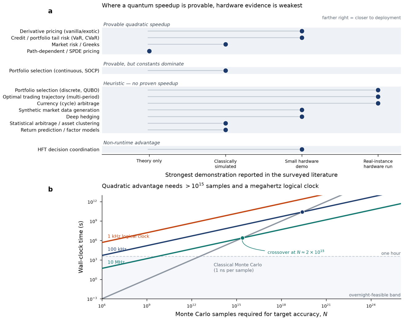
Table 1.
Trading tasks addressed in the quantum literature, with the strongest speedup claim and the strongest demonstration reported for each. Maturity reflects the cited work rather than a systematic scoring of all publications in each area; Appendix B gives the reported basis for each placement.
Table 1.
Trading tasks addressed in the quantum literature, with the strongest speedup claim and the strongest demonstration reported for each. Maturity reflects the cited work rather than a systematic scoring of all publications in each area; Appendix B gives the reported basis for each placement.
| Task | Algorithmic family | Speedup claim | Strongest demonstration | Ref. |
|---|---|---|---|---|
| Derivative pricing (vanilla/exotic) | Amplitude estimation | Quadratic in | Small hardware demo | [7] |
| Credit / portfolio tail risk (VaR, CVaR) | Amplitude estimation | Quadratic in | Small hardware demo | [8] |
| Market risk / Greeks | Amplitude estimation + gradient | Quadratic in and in #greeks | Classically simulated | [9] |
| Path-dependent / SPDE pricing | Quantum multilevel Monte Carlo | Theory only | [10] | |
| Portfolio selection (continuous, SOCP) | Quantum interior point | Polynomial, constants dominate | Classically simulated | [11] |
| Portfolio selection (discrete, QUBO) | Annealing / QAOA / VQE | Heuristic, none proven | Real-instance hardware run | [12] |
| Optimal trading trajectory (multi-period) | Annealing / QUBO | Heuristic, none proven | Real-instance hardware run | [13] |
| Currency (cycle) arbitrage | Annealing / QAOA | Heuristic, none proven | Real-instance hardware run | [14] |
| Synthetic market data generation | QGAN / Born machine | None proven | Small hardware demo | [17] |
| Deep hedging | Variational RL / policy | None proven | Small hardware demo | [18] |
| Statistical arbitrage / asset clustering | GBS, graph heuristics | Heuristic, none proven | Classically simulated | [15] |
| Return prediction / factor models | Quantum kernels, QNN | None; dequantized | Classically simulated | [16] |
| HFT decision coordination | Nonlocal games (entanglement) | Strategic, not runtime | Small hardware demo | [19] |
Disclaimer/Publisher’s Note: The statements, opinions and data contained in all publications are solely those of the individual author(s) and contributor(s) and not of MDPI and/or the editor(s). MDPI and/or the editor(s) disclaim responsibility for any injury to people or property resulting from any ideas, methods, instructions or products referred to in the content. |
© 2026 by the authors. Licensee MDPI, Basel, Switzerland. This article is an open access article distributed under the terms and conditions of the Creative Commons Attribution (CC BY) license.
Copyright: This open access article is published under a Creative Commons CC BY 4.0 license, which permit the free download, distribution, and reuse, provided that the author and preprint are cited in any reuse.