

Submitted:
21 August 2026
Posted:
21 August 2026
You are already at the latest version
Abstract
Steady compressible magnetohydrodynamic (MHD) boundary layers have been studied since the work of Rossow [32], Bleviss [3] and Bush [5]. What has not been developed is their unsteady similarity structure. This paper supplies it, by combining the Howarth--Dorodnitsyn transformation with the diffusion-time similarity ansatz of Sun [37], and in doing so uncovers a control mechanism that the steady literature did not isolate. Taking the applied field normal to the wall, B \( = B_0(x)\hat{e}_y \), makes the current solenoidal identically in two dimensions, so no auxiliary electrostatic problem arises. The external circuit is characterised by the classical load factor \( k = -E_z/(UB_0) \) [29,38]. The reduction yields a coupled pair of equations in \( (\eta,\tau) \) for the reduced stream function f and reduced total enthalpy g, governed by \( (a,b,c;\Theta,\mathrm{Pr},N,k) \) with \( N=\sigma B_0^2\delta^2/(C\mu_r) \) a squared Hartmann number. Our central structural result is that the load factor cancels identically from the momentum equation once the outer pressure field is treated consistently, and survives only in the enthalpy equation, where the combined Lorentz work and Joule dissipation reduce exactly to J\( \cdot\boldsymbol{E} \) \( =\sigma B_{0}^{2}kU\left(kU-u\right) \). The momentum source is \( N\omega(1-f_\eta) \) for every k; the enthalpy source is \( NE\,\omega\,k(k-f_\eta) \). Three consequences follow. (i) The linear Crocco integral survives the field only at k=0, where the classical \( g\equiv1 \) holds exactly despite an arbitrarily strong field, and at k=1, where it holds only for the cooled wall \( T_w/T_e = 2-\Theta \); for all other k no linear enthalpy--velocity relation exists. (ii) Because \( k(k-f_\eta) \) changes sign at \( f_\eta = k \), a boundary layer operating in generator mode extracts enthalpy near its outer edge. (iii) Consequently the load factor is a thermal-control parameter: sweeping k moves the adiabatic recovery factor from r=0.336 (a 44%reduction in adiabatic wall temperature relative to the field-free value at Me=4, N=4) through r=1 near \( k_*\simeq0.61 \) and on to thermal runaway, with an optimum cooling load factor \( k_{\rm opt}\simeq0.26 \) that is almost independent of N and is predicted analytically by \( k=f_\eta/2 \). The unsteady analysis gives three further results. The change of type of the reduced system is purely kinematic: both equations carry the same factor \( 1-c\tau f_\eta \), so \( \tau_{\rm crit}=1/c \) is independent of N, k, Mach number, Prandtl number and wall condition, while the thermal mode diverges beyond it a factor 1/Pr faster — confirmed by a \( 10^{44} \) disparity in computed divergences. Exact constancy of the compressibility parameter \( \Theta \) requires \( m=0 \) whereas unconditional well-posedness requires \( m\ge1 \), so the two are mutually exclusive. And for Pr=1 we derive and verify to seven digits the identity \( r = 2f_{\eta\eta}(0)Q-1 \) with \( Q=\int_{0}^{\infty}\exp\left[-\int_{0}^{\eta}f\right]d\eta \). Global solutions in the Williams--Rhyne chart connect the impulsive-start Rayleigh state to the steady state through the region forward marching cannot enter, and confirm that neither field nor compressibility is felt at the impulsive start.
Keywords:
unsteady compressible MHD boundary layers
; load-factor control
; similarity structure
; Howarth–Dorodnitsyn transformation
; enthalpy source
1. Introduction
1.1. Background and Prior Work
The boundary layer of an electrically conducting fluid in an applied magnetic field has a long history. In the incompressible case the Lorentz force enters the momentum balance as a linear Rayleigh-type drag and produces the Hartmann layer, with thickness and a characteristically full velocity profile [10,16,23,25,26,33]. Similarity solutions for magnetohydrodynamic (MHD) Falkner–Skan and stagnation-point flow were given by Neuringer and McIlroy [27] and have been extended in many directions since [1,8,28].
The compressible problem is also classical, and it is important to state clearly what is already known. Rossow [32] treated the conducting flat plate with a transverse field and recognised that the results depend on whether the field is fixed relative to the plate or to the fluid — the distinction that is formalised below as the load factor. Bleviss [3] analysed magnetogasdynamic Couette flow, and Bush [5] gave what is essentially the steady limit of the system studied here: compressible flat-plate boundary-layer flow with an applied magnetic field, including the coupling of Joule heating to the thermal field. Resler and Sears [29] set out the magneto-aerodynamic framework, including the accelerator/generator distinction. More recent work has addressed adverse pressure gradients and mass transfer [42,43], stability [7,40], rarefaction [22], the validity of the low- assumption for hypersonic control [11], and the rigorous well-posedness of the compressible MHD Prandtl system [18].
We therefore do not claim the steady effects of a magnetic field on a compressible boundary layer as new. That Joule dissipation raises the wall temperature, and that the transformed skin friction ceases to be Mach-independent once a field acts, are consequences that the 1957–1962 literature had the machinery to reach, and our steady computations should be read as recovering and quantifying them within a unified framework rather than discovering them.
1.2. What Is Missing, and What This Paper Adds
What that literature does not contain is the unsteady similarity structure. The unsteady compressible boundary layer has a rich theory of its own — the small-time Rayleigh–Stokes phase, the approach to the steady state, and Stewartson’s obstruction associated with the history terms [30,31,34,35,41] — and a similarity framework in diffusion-time variables has recently been given by Sun [37], building on Ma and Hui [24]. Applying that framework to a conducting fluid [14] exposes structure that the steady theory cannot see, because the obstruction, the relaxation behaviour and the history of the recovery factor are all intrinsically time-dependent.
Two reductions are combined here. The first casts the unsteady incompressible MHD problem in diffusion-time similarity form, in which the reduced momentum equation acquires a linear damping term and the unsteady terms group into , so that the coefficient can change sign. The second applies the same ansatz to the compressible problem after a Dorodnitsyn transformation. Their union is the subject of this paper.
Combining them also brings into focus a control parameter that the steady literature used but did not exploit systematically in a boundary-layer thermal context: the load factor k of the external circuit. Our main structural finding is that k cancels from the momentum equation and acts only on the enthalpy equation, which turns it into a clean thermal-control knob.
Contributions.
- 1.
- A closed unsteady master system (§Section 4) containing both parent problems as exact limits, with the field orientation chosen so that no electrostatic potential problem arises.
- 2.
- A load-factor decomposition theorem (§Section 3): the combined Lorentz work and Joule dissipation equal exactly; k cancels from momentum and survives only in the enthalpy source, whose sign structure permits net extraction of enthalpy from the layer.
- 3.
- A complete classification of magnetic Crocco integrals (§Section 6.1): survival only at (classical , exact for all and all N) and at (with the selected wall ).
- 4.
- A kinematic change-of-type theorem (§Section 5.1) with thermal amplification , and an incompatibility theorem (§Section 5.2) between exact similarity and unconditional well-posedness.
- 5.
- An exact recovery identity (§Section 6.3) and a load-factor map of the thermal state (§Section 8.3), including an optimum cooling load factor predicted analytically and confirmed numerically.
2. Formulation
2.1. Governing Equations and the Low- Approximation
Consider two-dimensional unsteady flow of a compressible, electrically conducting, calorically perfect gas over a wall at , with an external inviscid stream and edge conditions , , . Let be the electrical conductivity, the dynamic viscosity, k the thermal conductivity, the specific heat, and .
We work throughout at low magnetic Reynolds number,
which is the relevant regime for liquid metals, seeded combustion gases and moderately ionised hypersonic flows [25,38]. The induced magnetic field is then negligible compared with the applied field, the magnetic field is prescribed rather than solved for, and Ohm’s law in the quasi-static form reads
with and .
2.2. Orientation of the Applied Field
Two orientations are compatible with a two-dimensional boundary layer: a wall-normal field and a spanwise field . They are not equivalent, and the choice materially affects how much work is required to close the momentum equation.
Wall-normal field (adopted here).
With and , the motional electromotive force is , so the current is purely spanwise, with
Because nothing depends on z, the solenoidality condition reduces to , which is satisfied identically. No electrostatic potential problem arises: is set by the external circuit. Following standard magneto-aerodynamic practice [29,38] we parametrise that circuit by the load factor
whence the streamwise Lorentz force density is
Three cases are distinguished classically: is the short-circuited layer, in which no electric field is applied and the force opposes the motion everywhere; is generator operation; is the matched or unit-load condition, for which the free-stream current vanishes and the force acts only inside the layer, accelerating the retarded fluid; and is accelerator operation. Rossow’s distinction [32] between a field fixed to the plate and one fixed to the fluid is the special case versus . Much of the compressible literature [5,22] works at ; we retain general k throughout, because §Section 3 shows it to be the natural thermal-control parameter.
Spanwise field (for comparison).
With one finds , so the current has components in both x and y. Solenoidality is no longer automatic and one must solve subject to wall and far-field electrical boundary conditions. For perfectly insulating walls the net cross-stream current must vanish, and after elimination of the streamwise force reduces to the same functional form as (5) but with an orientation-dependent constant absorbed into the interaction parameter. Everything that follows therefore applies to both cases with N rescaled; we adopt the wall-normal field because it requires no auxiliary elliptic solve.
Remark 1.
The conductivity of a real gas depends strongly on temperature. Our baseline takes constant, appropriate to a liquid metal or a seeded gas at fixed ionisation fraction. A one-parameter generalisation is accommodated at no cost: every occurrence of ω below is replaced by (see Remark 4).
2.3. Boundary-Layer Equations with Electromagnetic Terms
At high Reynolds number the usual scaling gives , so across the layer. Evaluating the momentum equation at the edge, where , gives
so for the outer stream itself carries current and the pressure gradient is modified. Only at the matched condition is the ordinary compressible Bernoulli relation recovered unchanged. It is essential to retain (6); doing so produces the cancellation of Theorem 1. The equations are
where is the total enthalpy. Boundary conditions are at with either or , and , as .
3. The Load-Factor Decomposition Theorem
The two electromagnetic terms in () are usually carried separately, and the load factor is usually thought of as affecting both the momentum and the energy balance. Both impressions are misleading.
Theorem 1
(Load-factor decomposition). For any load factor k, with the outer pressure field determined consistently by (6):
- (i)
-
the total electromagnetic acceleration appearing in the momentum equation iswhich isindependent of k;
- (ii)
-
the total electromagnetic contribution to the total-enthalpy equation iswhich does depend on k, and changes sign across the layer at .
Proof. (i) From (6), . Adding and dividing by ,
The terms in k cancel identically: the current carried by the outer stream contributes a streamwise pressure gradient that exactly offsets its own contribution to the force inside the layer.
(ii) With and , and , so
which equals . The factor vanishes at and changes sign there. □
This is the organising result of the paper. The physical reading is that is the rate at which the external circuit delivers power to the fluid, and the load factor controls that delivery without altering the mechanical problem at all. Three regimes follow.
Corollary 1
(Short-circuited layer, ). When no electric field is applied, : the Lorentz force extracts mechanical energy at exactly the rate at which Joule dissipation returns it as heat, and the total-enthalpy equation is untouched by the field even though the momentum equation is not.
Corollary 2
(Generator operation, ). The source is positive where , i.e. in the inner part of the layer, andnegativewhere , i.e. in the outer part. The layer therefore delivers net electrical power to the circuit over part of its thickness, and its enthalpy is correspondingly depressed. §Section 8.3 shows this to be a large effect.
Corollary 3
(Matched and accelerator operation, ). For we have throughout, so everywhere: the layer acts as a distributed motor and heater simultaneously. At , .
4. Similarity Reduction and the Master System
4.1. Dorodnitsyn Variables
Introduce the Howarth–Dorodnitsyn normal coordinate and the Chapman–Rubesin approximation [6],
with reference state and C the Chapman–Rubesin constant. Since across the layer, exactly. Defining the compressible stream function through and V the transformed normal velocity, (7)–() become
Note that both the pressure-gradient term and the electromagnetic terms acquire the same temperature weighting: every body-force-like term in a compressible boundary layer is multiplied by the local density ratio (equivalently ). This is the single structural statement from which everything below follows.
4.2. Diffusion-Time Similarity Ansatz
Let be a diffusion length scale and set
so that . With and define
and the reduced static temperature
The geometric coefficients are
and the magnetic interaction parameter is
a squared Hartmann number built on the diffusion thickness. Since , an equivalent form is , which may be evaluated anywhere across the layer.
4.3. The Master System
Carrying out the reduction yields the coupled pair

with given by (17). Boundary conditions for a stationary wall beneath a stream are
together with either (isothermal) or, for an adiabatic wall, .
Remark 2
(Parent problems recovered). Setting gives , , , and (Section 4.3) collapses to the incompressible unsteady MHD equation . Setting recovers the unsteady compressible system exactly. The joint system contains both.
Remark 3
(Structure of the source). By Theorem 1 the electromagnetic terms in (Section 4.3)–(Section 4.3) are
so that is common to every circuit while carries all the k-dependence. Only at are the two proportional, ; this is the lever used in §Section 6.1. At the enthalpy source vanishes identically.
Remark 4
(Temperature-dependent conductivity). If then and the substitution in carries every result below through unchanged in form. The baseline is used in all computations.
4.4. Admissible Similarity Families
Similarity requires a, b, c, N, and to be independent of x. For a power-law stream with
the definitions (18) give the standard Falkner–Skan gauge
Constancy of N requires , hence
uniform only at the plane stagnation point . Constancy of requires a constant edge Mach number, which for an isentropic outer flow with holds exactly only for . These two requirements pull in opposite directions, a tension made precise in §Section 5.2.
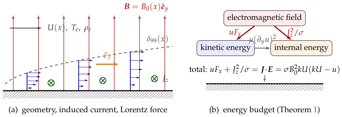
Figure 1.
Configuration and energy pathways. (a) A wall-normal applied field drives a purely spanwise current , where is the load factor of the external circuit. Because identically in two dimensions, no electrostatic potential problem arises. The matched condition is drawn: the current then vanishes in the free stream and the Lorentz force is positive, accelerating the retarded fluid and producing the characteristically full Hartmann profile. (b) The two electromagnetic channels sum exactly to the power delivered by the circuit, shown here for . By Theorem 1 the load factor cancels from the momentum balance and governs only this energy exchange, which reverses sign over the outer layer when and vanishes identically at .
Figure 1.
Configuration and energy pathways. (a) A wall-normal applied field drives a purely spanwise current , where is the load factor of the external circuit. Because identically in two dimensions, no electrostatic potential problem arises. The matched condition is drawn: the current then vanishes in the free stream and the Lorentz force is positive, accelerating the retarded fluid and producing the characteristically full Hartmann profile. (b) The two electromagnetic channels sum exactly to the power delivered by the circuit, shown here for . By Theorem 1 the load factor cancels from the momentum balance and governs only this energy exchange, which reverses sign over the outer layer when and vanishes identically at .
5. Structural Consequences
5.1. Change of Type Is Purely Kinematic
Both equations carry the same coefficient
Theorem 2
(Kinematic threshold). The master system is well posed as an initial-value problem in τ so long as throughout the layer. Since with at the edge, the first loss of parabolicity occurs at the boundary-layer edge at
independently of N, , , the wall thermal condition and the conductivity law. For , i.e. , the threshold is never reached and the march is unconditionally well posed.
Proof.
The threshold is determined solely by the sign of the coefficient of the -derivative, which is in both equations. Neither N nor , E, nor the boundary data appear in that coefficient. The supremum of over the layer is 1, attained as . □
Although the threshold is untouched, the severity of the ill-posedness is not.
Proposition 1
(Thermal amplification). Linearising about a state with and inserting a short-wave disturbance into the principal parts gives
For a gas with the thermal field is the more violently ill posed of the two, diverging a factor faster; for air, .
This is confirmed dramatically in §Section 8.4: past the threshold the wall shear reaches while the wall heat flux reaches .
Remark 5.
Theorem 2 corrects a natural expectation. One might suppose that a strong magnetic field, which suppresses the velocity defect and makes the profile fuller, would postpone the change of type. It does not: because the fieldraises throughout the interior, points inside the layer reach earlierthan they otherwise would. The field does not move the first crossing (which occurs at the edge, where regardless), but it makes the ill-posed region invade the interior faster.
5.2. An Incompatibility Theorem
Theorem 3
(No free lunch). Within the power-law family (23), exact constancy of the compressibility parameter Θ and unconditional well-posedness of the τ-march cannot hold simultaneously.
Proof.
Exact constancy of requires a constant edge Mach number. For an isentropic outer flow driven by , the edge temperature satisfies , so is constant only if U is, i.e. . By (23), gives and hence . Conversely, unconditional well-posedness requires , i.e. , for which U varies and cannot be constant. The two sets are disjoint. □
The practical consequence is that one must choose. The flat plate is the only exactly similar compressible member, and it is precisely the case in which Stewartson’s obstruction at appears; the stagnation point marches forever but requires the local-similarity interpretation for . We exploit both: §Section 8.5 uses for clean transients, and §Section 8.6 uses a global chart to solve despite the obstruction. Physically, requiring from (24) adds a third constraint, uniform field being admissible only at .
6. Exact Solutions and Integrals
6.1. The Magnetic Crocco Integral
Write both transport equations with the common operator
noting that reproduces exactly the non-source terms of (Section 4.3). At the dissipation term in (Section 4.3) vanishes and the pair reads
Theorem 4
(Classification of magnetic Crocco integrals). Let and , and let . Then solves (Section 4.3) for all τ if and only if the load factor takes one of two values:
- (a)
-
, with , giving theclassicalintegralvalid for arbitrarily strong fields and compatible with the adiabatic wall at rest;
- (b)
-
, with , givingwhich is compatible only with theisothermalwallrequiring ( for air).
For every other load factor no linear enthalpy–velocity relation exists.
Proof.
Since is linear and , substituting gives when . Requiring therefore demands
Cancelling , the polynomials and in must agree identically. Matching the coefficient of gives , and matching the constant term gives . Hence , so . For , and ; the far-field condition gives . For , and , whence using . □
Case (a) is striking and easy to overlook. At the magnetic field alters the velocity profile substantially — our computations give rising from at to at — yet the total enthalpy remains exactly uniform, , so that at the adiabatic wall recovers precisely the free-stream stagnation temperature and , just as in a non-conducting gas. We verify this to machine precision ( to double precision at ). The classical Crocco result is thus not destroyed by a magnetic field; it is destroyed by the applied electric field, and only when .
Two consequences are worth stating. First, when (33) holds the system decouples: g is known algebraically in terms of , and (Section 4.3) becomes a single closed PDE
an exact unsteady compressible MHD solution family for arbitrary N, and . Second, at the circuit selects the wall temperature. Without a field any linear Crocco relation is admissible and the adiabatic case is the celebrated one; at unit load factor only the single cooled wall (34) survives, and the adiabatic wall — which satisfies and hence would require — is not compatible. That incompatibility is the first sign of the effect developed in §Section 6.3.
6.2. Small-Time Limit and the Recovery Factor
As the diffusion terms are while , b and N terms are , so the field is not felt at leading order. With the momentum equation reduces to , giving the impulsive-start Rayleigh solution . Writing , the enthalpy equation reduces to a remarkably compact form.
Proposition 2.
At leading order as ,
with . For an adiabatic wall at rest, , and the quadrature evaluates in closed form to
for the recovery factor defined by .
Proof.
Substituting into the leading-order enthalpy balance and using collapses the dissipation terms to , giving (37). Integrating with ,
Polar substitution , over gives the double integral as . Using and produces (38); the factors of cancel identically, so is independent of Mach number. □
Two points follow. Expression (38) coincides with the value known for the impulsively moved plate in a gas at rest, so the same closed form governs the opposite configuration treated here. And, by Proposition 2, is independent of N: however strong the field, the recovery factor begins its history at the field-free value, for . Everything the field does to r, it does later. Our computations give (Table 7), a check on the global solver.
6.3. An Exact Steady Identity at
Theorem 5
(Recovery identity). For the steady flat plate (, , ) at unit load factor , with and an adiabatic wall at rest,
and whenever , so that .
Proof.
The steady momentum equation gives , so the energy equation becomes . Setting yields , whose solutions are spanned by 1 and , . Hence . The condition gives ; the adiabatic condition with gives . Evaluating at where gives , which is (39); the recovery factor follows from and .
For the inequality, integrate to get . Using ,
and the double integral is strictly positive because and . Hence with . □
At the identity degenerates gracefully: the Blasius relation gives exactly, so , recovering the classical result. Our computations return at and reproduce (39) to six decimal places for all N and tested (Table 4).
Corollary 4
(Adiabatic walls are singular in MHD). Because Joule dissipation is a volumetric source that an adiabatic wall cannot reject, the wall enthalpy must rise until convection alone removes the deposited power. Combining with the Hartmann estimate and gives the self-consistent strong-field balance and : the adiabatic wall temperature grows without bound with field strength. The constant-property assumptions underlying the model fail long before this limit, but the trend is real and is the dominant design consideration for MHD flow-control surfaces.
7. Numerical Method
Three solvers are used, each validated against the other two where they overlap.
- (i)
-
Steady two-point boundary-value solver.The steady limit of (Section 4.3)–(Section 4.3),is written as a five-dimensional first-order system (eliminating from the dissipation term) and solved by collocation with adaptive mesh refinement to a tolerance of . Solutions are continued in N from , each solution seeding the next; without continuation the solver readily jumps to spurious branches with at moderate N, and all results reported here were checked for pointwise positivity of .
- (ii)
-
Unsteady marching solver.Equations (Section 4.3)–(Section 4.3) are marched in using second-order backward differentiation (implicit Euler on the first step) and second-order central differences in , with Picard sweeps and tridiagonal solves alternating between and g to a tolerance of . The adiabatic wall condition is imposed with a ghost node, preserving second-order accuracy. The march is started at from the leading-order similarity state of §Section 6.2, obtained by solving (37) to machine precision; the resulting start-up error is verified by , which returns on and on .
- (iii)
-
Williams–Rhyne global solver.For the march is obstructed at . We therefore adopt the Williams–Rhyne chart [41]in which both and are characteristic, so that the whole history is obtained as one boundary-value problem in the strip with no marching at all. The transformed system iswith , , , and . Both and vanish at and . The limits are carried automatically: at one obtains , i.e. ; at , , , and the steady system (40) is recovered under , . The discrete residual on a grid () is driven below by a Newton–Krylov iteration with LGMRES inner solves, continued in N.
Cross-validation.
Table 1 collects checks against independently known values. The agreement with both parent theories is to five or six significant figures throughout.
The Hartmann-asymptote entry deserves a word: the incompressible strong-field expansion predicts , which for , , gives , matched to seven digits. This is a stringent test of the momentum discretisation in the regime where the Hartmann layer is thinnest.
8. Results
Throughout, and unless stated otherwise.
8.1. Steady Structure and the Loss of Mach-independence
Figure 2 and Table 2 present the central steady result. In the absence of a field the transformed flat-plate momentum equation is exactly Blasius, independent of : this Mach-independence in the Dorodnitsyn plane is one of the most useful features of classical compressible boundary-layer theory. The magnetic field destroys it.
The reason is structural. In the transformed momentum equation the Lorentz term is , and is not unity in a compressible gas. The sign of the effect is set by a competition, which explains the non-monotonic behaviour in Fig. Figure 2(c):
- Weak field. The force acts across the whole layer, where ranges from at the wall to (at ) at the edge. The layer-averaged is therefore below unity, the effective Lorentz force is weaker than in an incompressible fluid at the same N, and the wall shear falls below its incompressible value.
- Strong field. The force concentrates in a Hartmann layer at the wall, where ; moreover Joule dissipation raises the interior temperature substantially. The peak of grows from at to , and at , 25 and 100 (with rising from to ). The effective force is now stronger than incompressible and the shear exceeds it.
The crossover occurs near . The strong-field prefactor in Fig. Figure 2(d) makes the mechanism quantitative: it converges to at , confirming the incompressible asymptote, but to , and at , 4, 6, tracking the growth of rather than the wall value . In words:
Joule heat lightens the gas; a lighter gas feels a larger Lorentz acceleration per unit mass; a larger acceleration steepens the wall shear, which increases the current defect and hence the Joule heat.
This positive feedback loop has no counterpart in constant-density MHD, where by construction. It is the essential new mechanism of the joint problem.
8.2. Recovery Factors Above Unity
For a non-conducting gas the adiabatic-wall recovery factor is bounded by simple classical values: for the steady flat plate, and exactly at , the statement that an adiabatic wall recovers the free-stream stagnation temperature and no more. Joule dissipation breaks this bound, because it injects energy that did not come from the kinetic energy of the stream.
Figure 3.
Recovery factor of the steady adiabatic flat plate. (a) r against N for ; the inset resolves the crossing of near . (b) Verification of the exact identity of Theorem 5: thick pale curves are , open symbols are r computed directly from the wall temperature; the two agree to six decimals. (c) r against at : the black curve is the small-time closed form (38), the dashed curve the classical steady , and the coloured curves the steady values at increasing N. (d) The resulting adiabatic wall temperature (logarithmic scale); dotted lines mark the field-free values, exceeded by an order of magnitude by .
Figure 3.
Recovery factor of the steady adiabatic flat plate. (a) r against N for ; the inset resolves the crossing of near . (b) Verification of the exact identity of Theorem 5: thick pale curves are , open symbols are r computed directly from the wall temperature; the two agree to six decimals. (c) r against at : the black curve is the small-time closed form (38), the dashed curve the classical steady , and the coloured curves the steady values at increasing N. (d) The resulting adiabatic wall temperature (logarithmic scale); dotted lines mark the field-free values, exceeded by an order of magnitude by .
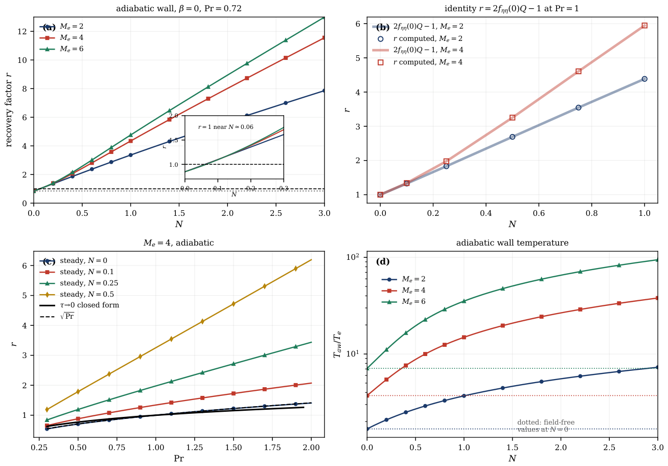
Table 3 shows r passing through unity near for every Mach number, and reaching an order of magnitude by . The corresponding adiabatic wall temperatures are severe: at and the wall sits at 35 times the edge static temperature, against without a field. Since r is defined against the stagnation-temperature rise, values mean literally that the surface is hotter than the stagnation temperature of the oncoming stream—an outcome impossible in non-conducting aerodynamics and controlled entirely by the interaction parameter.
Table 4 verifies Theorem 5 numerically. The agreement between the geometric quantity , computed from the momentum solution alone, and the thermodynamic quantity r, computed from the wall temperature, is to six decimal places over the whole range.

Table 4.
Verification of the exact identity of Theorem 5; steady flat plate, , adiabatic wall.
| N | Q | r (direct) | ||||
|---|---|---|---|---|---|---|
| 2 | ||||||
| 2 | ||||||
| 2 | ||||||
| 2 | ||||||
| 4 | ||||||
| 4 | ||||||
| 4 | ||||||
| 4 |
8.3. Load-factor Control of the Thermal State
Theorem 1 says the load factor is a pure thermal actuator: it leaves the momentum problem untouched and acts only on the enthalpy source. Figure 4 and Table 5 map the consequence.
Four features stand out.
The optimum is analytically predictable.
The enthalpy source is, at each station, minimised over k at , i.e. at . Since sweeps across the layer, a single load factor cannot be optimal everywhere, and the best compromise should lie near half the layer-averaged velocity ratio, i.e. –. The computed optima are – across a sixteen-fold range of N (Table 5), in good agreement, and the near-invariance of with N follows because enters the criterion but N does not.
The cooling is large.
At the adiabatic wall temperature falls from without a field to at . Since sets the equilibrium load on a thermal protection system, a reduction is of direct engineering interest, and it is achieved not by removing heat but by converting part of the layer’s enthalpy into electrical power delivered to the external circuit — the boundary layer operating as a distributed generator. This is the practically useful face of Corollary 2.
The heating and cooling regimes are separated sharply.
The crossing occurs at –, drifting slowly downward with N. Below the wall is cooler than the stagnation temperature; above it, hotter. Note that : the matched condition , which much of the compressible MHD literature adopts by default, sits well inside the heating regime and is close to the worst case rather than a neutral choice.
There is a runaway boundary.
Beyond no steady solution with throughout could be continued, and contracts from at to at . This is the finite-k expression of the adiabatic singularity noted after Theorem 5: an adiabatic wall cannot reject volumetric heat, so beyond a critical delivery rate the balance between Joule deposition and convective removal cannot be struck. We do not claim is a sharp turning point of the exact problem — resolving that would require arclength continuation — only that our continuation fails there and that the failure moves systematically with N.
8.4. The Change of Type, Numerically
Figure 5 tests the theory directly. Below the threshold the solutions are grid-converged: at the wall shear agrees to six significant figures on meshes of 1600, 3200 and 6400 points. Above it the solutions diverge at mesh-dependent times, the finer meshes surviving slightly longer—the signature of an ill-posed problem rather than a coding error, since refinement does not converge but merely postpones. The threshold itself is insensitive to N and : repeating the experiment at , gives the same , confirming Theorem 2. The disparity between panels (a) and (b) confirms Proposition 1: with the thermal growth rate exceeds the momentum growth rate by a factor , which compounded over the post-threshold interval produces the enormous separation observed.
8.5. Transients at the Stagnation Point
Figure 6 uses the stagnation point, where makes the march unconditionally well posed, to display complete transients. Three features are worth noting.
First, all wall-shear histories collapse onto at small , independently of N: the field is not felt until , as predicted in §Section 6.2. Second, the shear is non-monotonic: it undershoots its steady value before recovering, a feature inherited from the non-magnetic stagnation transient and amplified by the field. Third, and most important, the approach to the steady state is now controlled by the thermal field rather than the momentum field.
Table 6 makes this quantitative. In the incompressible problem the magnetic field monotonically accelerates the approach to the steady state, with , because magnetic damping adds a relaxation rate to viscous diffusion. Here the behaviour is non-monotonic: first rises, peaking near at more than twice its field-free value, before falling again at large N. The explanation is that an adiabatic wall must accumulate the Joule heat until convection can balance it, and that thermal accumulation is slow. At small N the extra heat load grows faster than the magnetic damping rate and the system takes longer to equilibrate; at large N the Hartmann damping eventually dominates and the classical acceleration returns. In compressible MHD it is thermal, not momentum, relaxation that sets the settling time over a wide intermediate range of field strengths—a point of direct practical relevance for pulsed or switched magnetic actuation.
8.6. Global Histories in the Williams–Rhyne Chart
The flat plate is the only exactly similar compressible member of the family (Theorem 3) and is precisely the case forward marching cannot complete. Figure 7 and Table 7 give the global solutions.
The table isolates the paper’s two main numerical claims in a single place. The column is constant at (against the exact , a discretisation error) for every N and , confirming that neither field nor compressibility is felt at the impulsive start. The column is likewise constant at against the closed form . At the other end, is identical for when —Mach-independence—but differs by between and at and by at . Meanwhile crosses unity between and , consistent with the steady computation of Table 3.
Table 7.
Williams–Rhyne global solutions, , adiabatic wall, ; is the impulsive start and the steady state. Note that and are independent of both N and , and that is Mach-independent at only.
Table 7.
Williams–Rhyne global solutions, , adiabatic wall, ; is the impulsive start and the steady state. Note that and are independent of both N and , and that is Mach-independent at only.
| N | |||||
|---|---|---|---|---|---|
| 0 | — | — | |||
| 0 | — | — | |||
| 0 | — | — | |||
| 2 | |||||
| 2 | |||||
| 2 | |||||
| 2 | |||||
| 2 | |||||
| 4 | |||||
| 4 | |||||
| 4 | |||||
| 4 |
Panel (a) of Fig. Figure 7 deserves particular attention: it maps over the whole strip and shows that a substantial part of the physically relevant history—everything to the right of the heavy contour, which the vertical dotted line at first touches—is inaccessible to any forward-marching scheme, however refined. The global chart obtains it as an ordinary boundary-value problem.
9. Discussion and Limitations
What is new, and what is not.
We separate these carefully. The steady effects of §Section 8.1–§Section 8.2 — loss of Mach-independence of the transformed skin friction, and Joule-driven wall heating — lie within reach of the classical steady analyses of Rossow [32] and Bush [5], and we present them as recovered and quantified within a unified framework, not as discoveries. Their value here is that the same solver reproduces both parent limits to six figures, which underwrites the unsteady results.
What we believe to be new is: (i) the load-factor decomposition (Theorem 1), namely that k cancels from momentum once the outer pressure field is treated consistently and survives only in the enthalpy source; (ii) the resulting classification of magnetic Crocco integrals into exactly two admissible load factors (Theorem 4), including the exact survival of at under arbitrarily strong fields; (iii) the load-factor map of the thermal state with its analytically predicted optimum (§Section 8.3); (iv) the kinematic change-of-type theorem with its thermal amplification (§Section 5.1); (v) the incompatibility theorem (§Section 5.2); and (vi) the recovery identity (§Section 6.3). Items (iv)–(vi) have no steady analogue at all. Underlying the compressible–magnetic coupling throughout is that the Lorentz acceleration per unit mass carries a factor T, so a temperature field partly generated by the field feeds back into the momentum balance.
Range of validity.
The results rest on four approximations. (a) Low . The induced field is neglected; for the field must be solved for and the closure (4) fails. (b) Constant σ and Chapman–Rubesin C. This is the weakest assumption, and it is weakest precisely where we push hardest: at –6 the gas conducts because it is hot, and then varies by orders of magnitude across the layer. Remark 4 shows how a power law is absorbed without changing the form of any result, and since the feedback loop of §Section 8.1 would strengthen; but the quantitative values at should be read as indicative of trend, not as predictions. A fully coupled ionisation model is the obvious next step. (b′) Prescribed load factor. We treat k as an externally imposed constant. A real electrode arrangement fixes the terminal voltage, not k pointwise, and end effects near electrode edges are outside the boundary-layer framework. (c) Laminar flow. At the interaction parameters where , the combination of strong wall heating and a Hartmann-thinned layer would in practice interact with transition; the field is known to be stabilising, but the laminar assumption is a genuine restriction. (d) The adiabatic idealisation. As the corollary to Theorem 5 shows, an adiabatic wall with volumetric heating is a singular limit whose temperature grows without bound with N. Real surfaces radiate and conduct; the adiabatic results should be read as an upper envelope, valuable because they bound the thermal load, not as a prediction of attainable wall temperature.
Relation to prior work.
The incompressible limit reproduces the known unsteady MHD reduction including its change of type and Hartmann asymptote; the field-free limit reproduces the unsteady compressible theory including the Crocco integral, the recovery factor (38) and the Williams–Rhyne structure. The contribution here is the coupling and its consequences, of which Theorem 1 (the exact source), Theorem 4 (the selected wall) and Theorem 5 (the recovery identity) are the analytical core.
10. Conclusions
We have formulated and solved the unsteady compressible MHD boundary layer at low magnetic Reynolds number, with a wall-normal applied field chosen so that the current is solenoidal identically, and with the external circuit characterised by its load factor k.
- 1.
- Load-factor decomposition. Once the outer pressure field is determined consistently, k cancels identically from the momentum equation and survives only in the enthalpy equation, where the combined Lorentz work and Joule dissipation reduce exactly to (Theorem 1). The momentum source is for every circuit; the enthalpy source is , which changes sign at .
- 2.
- Two admissible Crocco integrals, and no others. A linear enthalpy–velocity relation survives only at , where the classical holds exactly for arbitrarily strong fields, and at , where it holds only for the cooled wall (Theorem 4). The classical Crocco result is destroyed not by the magnetic field but by the applied electric field.
- 3.
- The load factor is a thermal actuator. Sweeping k moves the adiabatic recovery factor from — a reduction in adiabatic wall temperature at , — through near and on to thermal runaway beyond . The optimum cooling load factor is nearly independent of N and is predicted by the pointwise criterion . The matched condition commonly adopted in the literature lies well inside the heating regime.
- 4.
- The change of type is purely kinematic. Both equations share the factor , so is independent of N, k, , and wall condition (Theorem 2), while the thermal mode diverges beyond it a factor faster (Proposition 1), confirmed by a disparity in computed divergences.
- 5.
- Exact similarity and unconditional well-posedness are incompatible within the admissible family (Theorem 3).
- 6.
- An exact recovery identity holds at , (Theorem 5) and is verified to six decimals.
- 7.
- Steady effects recovered. The loss of Mach-independence of transformed flat-plate skin friction ( at , at ) and Joule-driven wall heating are quantified within the same framework; these are consistent with, rather than additional to, the classical steady literature.
Natural extensions include a temperature-dependent conductivity coupled to an ionisation model; three-dimensional and swept configurations, where the spanwise orientation requires the electrostatic problem to be solved; finite- effects; arclength continuation to resolve the structure of the runaway boundary ; and the stability of these profiles, where the competition between Hartmann stabilisation [23,40] and the strongly modified thermal layer identified here — which the load factor can make either hotter or cooler than the field-free case — seems likely to be delicate [7].
Author Contributions
Bo Hua Sun: Conceptualization, Methodology, Formulations, Formal analysis, Funding acquisition, Investigation, Writing- Original draft preparation, Writing- Reviewing and Editing and all relevant works.
Data Availability Statement
Availability of data: The data supporting the findings of this study are available from the corresponding author upon reasonable request.
Acknowledgments
My investigations into the boundary layers started from my tenure as a professor at the Cape Peninsula University of Technology (CPUT), South Africa. I am profoundly grateful to CPUT for granting me complete academic autonomy to advance this research agenda. This vital institutional support laid the foundation for the principal conclusions presented in this manuscript. I also extend my deepest gratitude to former Vice-Chancellor (now Chancellor) Prof. Brian Figaji, and former Deputy Vice-Chancellors Prof. J. A. Tromp and Prof. Anthony Staak, for their generous support and endorsement. Further academic support was provided by Xi’an University of Architecture and Technology (XAUAT) and the Beijing Institute of Nanoenergy and Nanosystems (BINN), Chinese Academy of Sciences. I sincerely thank former XAUAT President Prof. Xiao-Jun Liu and current President Prof. Xiang-Mo Zhao, along with BINN Founding Director Prof. Zhong Lin Wang, for their unwavering encouragement and invaluable resource support throughout this study.
Conflicts of Interest
The authors declare that there are no competing financial interests.
References
- Abbasbandy, S.; Hayat, T. Solution of the MHD Falkner–Skan flow by homotopy analysis method. Commun. Nonlinear Sci. Numer. Simul. 2009, 14, 3591–3598. [Google Scholar] [CrossRef]
- Blasius, H. Grenzschichten in Flüssigkeiten mit kleiner Reibung. Z. Math. Phys. 1908, 56, 1–37. [Google Scholar]
- Bleviss, Z. O. Magnetogasdynamics of hypersonic Couette flow. J. Aero/Space Sci. 1958, 25(10), 601–615. [Google Scholar] [CrossRef]
- Bush, W. B. Magnetohydrodynamic-hypersonic flow past a blunt body. J. Aero/Space Sci. 1958, 25(11), 685–690. [Google Scholar] [CrossRef]
- Bush, W. B. Compressible flat-plate boundary-layer flow with an applied magnetic field. J. Aerosp. Sci. 1960, 27(1), 49–58. [Google Scholar] [CrossRef]
- Chapman, D. R.; Rubesin, M. W. Temperature and velocity profiles in the compressible laminar boundary layer with arbitrary distribution of surface temperature. J. Aeronaut. Sci. 1949, 16, 547–565. [Google Scholar] [CrossRef]
- Cheng, F.; Zhong, X.; Gogineni, S.; Kimmel, R. L. Magnetic-field effects on second-mode instability of a weakly ionized Mach 4.5 boundary layer. Phys. Fluids 2003, 15, 2020–2040. [Google Scholar] [CrossRef]
- Chiam, T. C. Hydromagnetic flow over a surface stretching with a power-law velocity. Int. J. Eng. Sci. 1995, 33, 429–435. [Google Scholar] [CrossRef]
- Crocco, L. Sulla trasmissione del calore da una lamina piana a un fluido scorrente ad alta velocità. L’Aerotecnica 1932, 12, 181–197. [Google Scholar]
- P. A. Davidson, <italic>An Introduction to Magnetohydrodynamics</italic>, Cambridge University Press, 2001.
- Study on validity of the low-magnetic-Reynolds-number assumption for hypersonic magnetohydrodynamic control. AIAA J. 2023. [CrossRef]
- Dorodnitsyn, A. A. Boundary layer in a compressible gas. Prikl. Mat. Mekh. 1942, 6, 449–486. [Google Scholar]
- Falkner, V. M.; Skan, S. W. Some approximate solutions of the boundary layer equations. Philos. Mag. 1931, 12, 865–896. [Google Scholar] [CrossRef]
- Fu, J.-Y.; Ni, M.-J.; Zhang, N.-M. Theoretical analysis for non-linear effects of magnetic fields on unsteady boundary layer flows. arXiv 2025, arXiv:2504.06576. [Google Scholar]
- Hall, M. G. The boundary layer over an impulsively started flat plate. Proc. R. Soc. Lond. A 1969, 310, 401–414. [Google Scholar] [CrossRef]
- Hartmann, J. Hg-dynamics I: theory of the laminar flow of an electrically conductive liquid in a homogeneous magnetic field. K. Dan. Vidensk. Selsk. Mat. Fys. Medd. 1937, 15, 1–28. [Google Scholar]
- Howarth, L. Concerning the effect of compressibility on laminar boundary layers and their separation. Proc. R. Soc. Lond. A 1948, 194, 16–42. [Google Scholar] [CrossRef]
- Huang, Y.; Liu, C.-J.; Yang, T. Local-in-time well-posedness for compressible MHD boundary layer. J. Differ. Equ. 2019, arXiv:1803.06681266, 2978–3013. [Google Scholar] [CrossRef]
- Illingworth, C. R. Steady flow in the laminar boundary layer of a gas. Proc. R. Soc. Lond. A 1949, 199, 533–558. [Google Scholar] [CrossRef]
- Kemp, N. H.; Petschek, H. E. Two-dimensional incompressible magnetohydrodynamic flow across an elliptic solenoid. J. Fluid Mech. 1958, 4, 553–584. [Google Scholar] [CrossRef]
- Lees, L. Laminar heat transfer over blunt-nosed bodies at hypersonic flight speeds. Jet. Propuls. 1956, 26, 259–269. [Google Scholar] [CrossRef]
- Compressible magnetohydrodynamic flat plate boundary layer flow with slightly rarefied effects. Eur. J. Mech. B/Fluids 2025. [CrossRef]
- Lock, R. C. The stability of the flow of an electrically conducting fluid between parallel planes under a transverse magnetic field. Proc. R. Soc. Lond. A 1955, 233, 105–125. [Google Scholar] [CrossRef]
- Ma, P. K. H.; Hui, W. H. Similarity solutions of the two-dimensional unsteady boundary-layer equations. J. Fluid Mech. 1990, 216, 537–559. [Google Scholar] [CrossRef]
- Moreau, R. Magnetohydrodynamics; Kluwer, 1990. [Google Scholar]
- Müller, U.; Bühler, L. Magnetofluiddynamics in Channels and Containers; Springer: Berlin, 2001. [Google Scholar]
- Neuringer, J. L.; McIlroy, W. Incompressible two-dimensional stagnation-point flow of an electrically conducting viscous fluid in the presence of a magnetic field. J. Aero/Space Sci. 1958, 25, 194–198. [Google Scholar] [CrossRef]
- Parand, K.; Rezaei, A. R.; Ghaderi, S. M. An approximate solution of the MHD Falkner–Skan flow by Hermite functions pseudospectral method. Commun. Nonlinear Sci. Numer. Simul. 2011, 16, 274–283. [Google Scholar] [CrossRef]
- Resler, E. L.; Sears, W. R. The prospects for magneto-aerodynamics. J. Aeronaut. Sci. 1958, 25, 235–245, 258. [Google Scholar] [CrossRef]
- Rhyne, T. B. The unsteady laminar boundary layer on a semi-infinite flat plate. PhD thesis, North Carolina State University, 1968. [Google Scholar]
- Riley, N. Unsteady laminar boundary layers. SIAM Rev. 1975, 17, 274–297. [Google Scholar] [CrossRef]
- Rossow, V. J. On flow of electrically conducting fluids over a flat plate in the presence of a transverse magnetic field. NACA Report 1358. 1957.
- Shercliff, J. A. A Textbook of Magnetohydrodynamics; Pergamon Press, 1965. [Google Scholar]
- Stewartson, K. On the impulsive motion of a flat plate in a viscous fluid. Q. J. Mech. Appl. Math. 1951, 4, 182–198. [Google Scholar] [CrossRef]
- Stewartson, K. The theory of unsteady laminar boundary layers. Adv. Appl. Mech. 1960, 6, 1–37. [Google Scholar] [CrossRef]
- Stewartson, K. The Theory of Laminar Boundary Layers in Compressible Fluids; Oxford University Press, 1964. [Google Scholar]
- Sun, B. H. Similarity solutions of a class of unsteady laminar boundary layer. Phys. Fluids 2024, 36, 083616. [Google Scholar] [CrossRef]
- Sutton, G. W.; Sherman, A. Engineering Magnetohydrodynamics; McGraw-Hill, 1965. [Google Scholar]
- Van Driest, E. R. NACA TN 2597; Investigation of laminar boundary layer in compressible fluids using the Crocco method. 1952.
- Watanabe, T. Magnetohydrodynamic stability of boundary layers along a flat plate in the presence of a transverse magnetic field. ZAMM 1978, 58, 555–560. [Google Scholar] [CrossRef]
- Williams, J. C., III; Rhyne, T. B. Boundary layers near a stagnation point of an impulsively started flow. SIAM J. Appl. Math. 1980, 38, 215–224. [Google Scholar]
- Xenos, M.; Kafoussias, N.; Karahalios, G. Magnetohydrodynamic compressible laminar boundary-layer adiabatic flow with adverse pressure gradient and continuous or localized mass transfer. Can. J. Phys. 2001, 79, 1247–1263. [Google Scholar] [CrossRef]
- Xenos, M.; Kafoussias, N. MHD compressible turbulent boundary-layer flow with adverse pressure gradient. Acta Mech. 2005, 180, 91–107. [Google Scholar] [CrossRef]
Figure 2.
Steady compressible MHD boundary layer, , isothermal wall , . (a) Velocity profiles at : the Lorentz force progressively fills the profile, collapsing it onto a Hartmann layer of thickness . (b) Static temperature: Joule dissipation builds an interior maximum that grows from at to at , with the peak migrating towards the wall as the current concentrates there. (c) Departure of the wall shear from its incompressible value. At the departure is identically zero for every Mach number; it becomes non-zero as soon as , dips about negative near , changes sign near and rises to by . (d) The strong-field friction prefactor , which tends to 1 in the incompressible limit but to values above 1 when the gas is compressible.
Figure 2.
Steady compressible MHD boundary layer, , isothermal wall , . (a) Velocity profiles at : the Lorentz force progressively fills the profile, collapsing it onto a Hartmann layer of thickness . (b) Static temperature: Joule dissipation builds an interior maximum that grows from at to at , with the peak migrating towards the wall as the current concentrates there. (c) Departure of the wall shear from its incompressible value. At the departure is identically zero for every Mach number; it becomes non-zero as soon as , dips about negative near , changes sign near and rises to by . (d) The strong-field friction prefactor , which tends to 1 in the incompressible limit but to values above 1 when the gas is compressible.
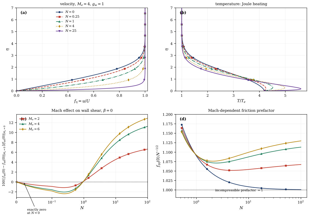
Figure 4.
The load factor as a thermal-control parameter; steady flat plate (), , , adiabatic wall. (a) Recovery factor against k; stars mark the minima. The shaded band is the cooling regime . All curves pass through a common neighbourhood near , and all fall below the field-free for . (b) The corresponding adiabatic wall temperature, which at , falls to against the field-free — a reduction. (c) The shape of the enthalpy source : identically zero at (Corollary 1), negative over the outer layer for (Corollary 2), and positive throughout for (Corollary 3). (d) Regime boundaries against N: the optimum cooling load factor is nearly independent of N, while the runaway boundary contracts sharply.
Figure 4.
The load factor as a thermal-control parameter; steady flat plate (), , , adiabatic wall. (a) Recovery factor against k; stars mark the minima. The shaded band is the cooling regime . All curves pass through a common neighbourhood near , and all fall below the field-free for . (b) The corresponding adiabatic wall temperature, which at , falls to against the field-free — a reduction. (c) The shape of the enthalpy source : identically zero at (Corollary 1), negative over the outer layer for (Corollary 2), and positive throughout for (Corollary 3). (d) Regime boundaries against N: the optimum cooling load factor is nearly independent of N, while the runaway boundary contracts sharply.
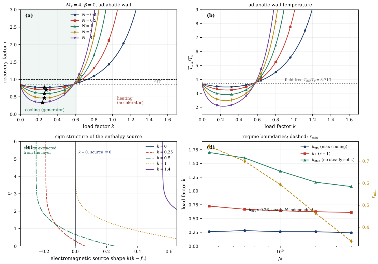
Figure 5.
Numerical confirmation of Theorem 2 and Proposition 1 for (, ), , . (a) Wall shear on four meshes: grid-converged to six figures before , mesh-dependent divergence immediately after. (b) Wall heat flux on the same meshes, reaching where the shear reaches : the thermal mode is the more violently ill posed, as predicted. (c) The parabolicity parameter , whose maximum reaches 1 at at the boundary-layer edge. (d) For () the same solver marches without difficulty on all meshes.
Figure 5.
Numerical confirmation of Theorem 2 and Proposition 1 for (, ), , . (a) Wall shear on four meshes: grid-converged to six figures before , mesh-dependent divergence immediately after. (b) Wall heat flux on the same meshes, reaching where the shear reaches : the thermal mode is the more violently ill posed, as predicted. (c) The parabolicity parameter , whose maximum reaches 1 at at the boundary-layer edge. (d) For () the same solver marches without difficulty on all meshes.
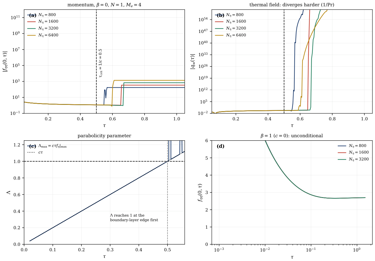
Figure 6.
Transients at the plane stagnation point (, unconditionally well posed), adiabatic wall, . (a) Velocity profiles at , , showing the transient overshoot characteristic of impulsively started stagnation flow. (b) Static temperature: the adiabatic wall accumulates Joule heat, rising from to nearly 9. (c) Wall shear histories, collapsing onto the Rayleigh law at small regardless of N. (d) The recovery factor, which begins at the field-independent value of Eq. (38) and migrates upward through for all .
Figure 6.
Transients at the plane stagnation point (, unconditionally well posed), adiabatic wall, . (a) Velocity profiles at , , showing the transient overshoot characteristic of impulsively started stagnation flow. (b) Static temperature: the adiabatic wall accumulates Joule heat, rising from to nearly 9. (c) Wall shear histories, collapsing onto the Rayleigh law at small regardless of N. (d) The recovery factor, which begins at the field-independent value of Eq. (38) and migrates upward through for all .
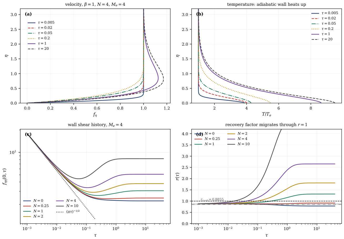
Figure 7.
Global solutions of the flat-plate problem (, ), adiabatic wall, , obtained as boundary-value problems in the Williams–Rhyne strip. (a) The parabolicity parameter in the plane; forward marching cannot enter the region right of the heavy contour, which the global chart traverses without difficulty. (b) Wall shear from the impulsive-start value to the steady state. (c) Recovery factor across the entire history, migrating from the field-independent value towards steady values that exceed unity for . (d) Solid curves () for are indistinguishable, confirming Mach-independence; dashed curves () separate clearly.
Figure 7.
Global solutions of the flat-plate problem (, ), adiabatic wall, , obtained as boundary-value problems in the Williams–Rhyne strip. (a) The parabolicity parameter in the plane; forward marching cannot enter the region right of the heavy contour, which the global chart traverses without difficulty. (b) Wall shear from the impulsive-start value to the steady state. (c) Recovery factor across the entire history, migrating from the field-independent value towards steady values that exceed unity for . (d) Solid curves () for are indistinguishable, confirming Mach-independence; dashed curves () separate clearly.
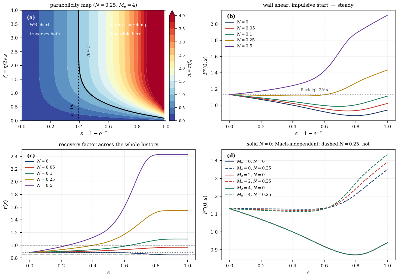
Table 1.
Validation of the three solvers against independently known results.
| Quantity | Condition | Computed | Reference |
|---|---|---|---|
| , , any | (Blasius–Dorodnitsyn) | ||
| , , | identical | ||
| , , | |||
| , , | (Falkner–Skan) | ||
| , , | (Hartmann asymptote) | ||
| unsteady march → steady, | (BVP solver) | ||
| WR chart, , | |||
| WR chart, any N, any | (Eq. (38)) | ||
| steady, , | 1 (Theorem 5) |
Table 2.
Wall shear for the steady flat plate (), isothermal wall , . The row is Mach-independent to all digits shown; every other row is not.
Table 2.
Wall shear for the steady flat plate (), isothermal wall , . The row is Mach-independent to all digits shown; every other row is not.
| N | spread | ||||
|---|---|---|---|---|---|
| 0 | |||||
| 1 | |||||
| 4 | |||||
| 25 | |||||
| 100 |
Table 3.
Adiabatic recovery factor r and wall temperature ratio for the steady flat plate, .
| r | ||||||
|---|---|---|---|---|---|---|
| N | ||||||
Table 5.
Load-factor map of the steady adiabatic flat plate, , . is the load factor of maximum cooling, that at which , and the largest load factor admitting a steady solution. The field-free values are and .
Table 5.
Load-factor map of the steady adiabatic flat plate, , . is the load factor of maximum cooling, that at which , and the largest load factor admitting a steady solution. The field-free values are and .
| N | at | |||||
|---|---|---|---|---|---|---|
Table 6.
Relaxation time (last at which differs from its steady value by more than ), , adiabatic wall, .
Table 6.
Relaxation time (last at which differs from its steady value by more than ), , adiabatic wall, .
| N | 0 | 1 | 2 | 4 | 10 | |
|---|---|---|---|---|---|---|
| () |
Disclaimer/Publisher’s Note: The statements, opinions and data contained in all publications are solely those of the individual author(s) and contributor(s) and not of MDPI and/or the editor(s). MDPI and/or the editor(s) disclaim responsibility for any injury to people or property resulting from any ideas, methods, instructions or products referred to in the content. |
© 2026 by the authors. Licensee MDPI, Basel, Switzerland. This article is an open access article distributed under the terms and conditions of the Creative Commons Attribution (CC BY) license (http://creativecommons.org/licenses/by/4.0/).
Copyright: This open access article is published under a Creative Commons CC BY 4.0 license, which permit the free download, distribution, and reuse, provided that the author and preprint are cited in any reuse.