
Submitted:
20 August 2026
Posted:
21 August 2026
You are already at the latest version
Abstract
A recent 2026 paper by Courbin and Maeder have demonstrated that the Hubble tension can be resolved within the Scale Invariant Vacuum (SIV) paradigm but they didn’t demonstrate that the CMB spectra would be correctly reproduced. In this paper, an equivalent but physically different idea using time Re-parameterization Invariant Scaling Symmetry (RISS) is utilized to build a model that resolves the Hubble tension without introducing new particles or fields. Here the Hubble tension is recognized to be due to difference in the unit of time during the decoupling and the current era since the corresponding gravitational potentials are different. This is justified by considering the SIV-like scaling factor using Newtonian gauge to define \( \lambda=N/N_0=\sqrt{(1+2\Psi)}/N_0 \). Then by introducing specific λ(a) a new gauge independent background reformulation is achieved since now λ depends on the expansion scale factor a that can be viewed as a specific time parametrization for the evolution of the Universe. The key is an epoch-dependent rescaling of the Hubble function \( H_{new}=\xi(a)^{-1}H_{std}(a) \). Finally, after adjustments to the main cosmology parameters one can reproduce the original LCDM CMB spectrum within less than a few percent for the individual ClTT values. The values of the new cosmology parameters are \( h=0.755, \Omega_m =0.248, \omega_b=\Omega_b h^2=0.0225, A_s=2.07\times10^{-9}, n_s=0.968,\tau_{rei}=0.0489 \).
Keywords:
cosmology
; Hubble tension
; CMB
; reparametrization
; weyl geometry
; dirac cosmology
MSC: 98.80.-k; 98.70.Vc; 98.80.Es; 95.36.+x; 04.50.Kd; 04.50.+h
1. Introduction
The Hubble Tension: The value of the Hubble constant determined via CMB processes during the decoupling epoch is different from the value seen at the current epoch . The ratio of the Planck predicted km/s/Mpc to the locally observed km/s/Mpc is 0.93 [1,2]. Initially this differences were considered a tension since it was a few discrepancy. However, with the improvement of the experimental uncertainties now it has become a problem at more than 5 discrepancy [3,4]. Even more, it has be identified as 6 difference but is also resolved within the Scale Invariant Vacuum (SIV) paradigm by modification to the Hubble function [5]. While the temperature () and the value of the Hubble expansion at decoupling are almost the same for SIV and LCDM ( see Figure 4 in [5]), the value of z at decoupling is different for the two models ( and ) as well as the value of is now 0.2 for SIV instead of 0.31 as for LCDM.
FFAT Scaling Symmetry Idea: The idea of rescaling suggested a possible resolution by looking into its impact on the Free-fall, Amplitude, and Thomson (FFAT) scaling [6] (see (2) for the currently adopted version). Subsequently, a study of various surrogate dark processes and matter components have been studied in details by [7,8]. The problem with such constant rescaling adjustment is that if it was present during the decoupling epoch it would manifest itself in the Thomson scattering today as well. It seems that a way out would be if the scaling is time dependent so that now but during the decoupling epoch it could have been different so it could affect the relevant processes and place its fingerprint as a different accordingly.
The Scale Invariant Vacuum (SIV) Idea: Within the SIV paradigm [9,10], there is an overall conformal factor that now is ; thus, there will be no effect on current measurements but in the past it could induce modifications. If one is to consider only time rescaling then one may have where is a time reparametrization factor. Since this is happening during the matter dominated epoch then one can use the corresponding functional form for within SIV given in dimensionless time with and to determine . The Big-Bang within SIV is happening near . Which for 5% and 30% gives 0.37 and 0.66 for . By setting , which is way too late than what is usually expected, and by using , one gets that seems to be at odds with the conventional matter content. However, when SIV is carefully applied, as shown in [5] one can first determine the for the SIV model, and then by looking at the one can show that one can arrive at within SIV that agrees with the local observations. Here the SIV framework is used but the above argument will be refined by implementing and subsequent modifications to that resolves the Hubble tension and shows that the CMB spectra can be properly recovered. The current framework also provides a physical interpretation of the scaling function within the RISS paradigm.
Reparametrization Invariant Scaling Symmetry (RISS) resolution: The RISS idea is very similar to the SIV framework mathematically [10,11,12], but differs in the freedom of choosing a time parametrization for the description of a physical process. Thus, has to be finalized given the process under consideration and the physical situation. For the discussion here, Cosmology and the CMB, will be related to the lapse function see Section 4. The physical situation is an evolving gravitational potential of the universe that at recombination is bigger than at the current epoch. Evolving gravitational potential is a key component in modern CMB computer codes (see Figure 1). However, one can understand such decrease towards its current value simply by looking at the gravitational potential within a homogeneous spherical mass/energy distribution. If R is the radius of the causally connected part of the Universe with total mass/energy M within R then one has – as the Universe expands R grows, but G and M stay the same within the usual view point. Thus, the gravitational potential decreases as the Universe expands! This effectively modifies the unit of time. The current resolution of the Hubble tension is related to such time unit adjustment between and as discussed in Section 4 and further validated by subsequent CMB calculations as demonstrated in Figure 3.
2. Key Expressions in Cosmology
Consider the Hubble function related to the expansion factor a, and the conformal time given by:
In the above expressions, t is considered to be the cosmic time, as such the proper time for the evolution of the Universe, when utilizing the FLRW cosmology. However, later t will be a time coordinate used by an observer, while the proper time for the evolution of the Universe will be denoted by with .
Dimensional considerations show that time-dependent re-scaling of units by satisfies re-parametrization invariance! Such rescaling can be generated by the change of the time unit, which induces change in the distance unit to maintain constant speed of light.
The rescaling of the Hubble function is related to the FLRW equations that define the background cosmology:
By using , these equations can be written in the standard form containing term. If time is introduced by integrating the relationship then scaling is naturally induced upon and can be used to induce changes in the units or it can be related to introducing a lapse function then for
To retain the speed of light unaltered then one has to either rescale the scale-factor or the spacial units to obtain a conformally equivalent metric . Thus, by re-scaling the unit of time () and keeping the speed of light fixed then one also should rescale the distance unit resulting in the rescaling of k, which has inverses distance units – usually Mpc−1 for cosmology considerations. Alternatively, one can consider a Weyl transformation only for N and a for a fixed coordinate system with fixed units. The first of these symmetries, related to units change, is obvious in the CMB equations [6,7,8] except for the term that is related to . While the second transformation does not affect the conformal time and many of the related terms. However, a special attention and discussion is needed for and .
Note that the time reparametrization may be broken in the second equation (3) related to the pressures since . This suggests considering to be related to a dark substance, which can be identified as pressure component . As such it can be related to early dark energy. Such terms appear upon generalization of the FLRW equations to reparametrization invariant form as part of the scale-invariant cosmology equations [10,11,12].
Let’s now consider the Weyl transformation along with ; one can think of it as , without change in the spacial units, as proxy to changing the lapse function N. Note that this is actually when related to the units rescaling discussed earlier (2). Such Weyl transformation does not affect the conformal time and k and keeps the equations almost invariant as well, but one has to look closely at the and terms. These terms are invariant upon constant rescaling, since , same for and due to the [T−2] units in G that offset the change , but for time-dependent one must revisit the FLRW equations. For time-dependent change, one has for :
thus, no change for the usual constant rescaling. However, if one defines then should be in proper time parametrization where must be constant. So, one should consider to be where is the proper time parametrization!
Let’s look at and other observables. Note that the Thomson opacity in conformal time is given by but it is in proper time, otherwise it is . Since the photon visibility function is with optical depth:
therefore, in proper time but in conformal time, as mentioned already. However, it should be in proper time for the description of the relevant processes. Therefore, here the view is to consider . This shows that is invariant even for time-dependent rescaling.
3. Symmetry Extended Cosmology
The idea of Scale Invariant Cosmology has been discussed by Eddington, Dirac, Canuto et al, and further pushed by Buvie and Maeder [14,15,16,17] within the context of cosmology and astrophysics. The theory is often and easily mistaken for some type of Jordan-Brain-Dike conformal theory due to the absence of clear delimitation of what is the physical meaning of the conformal factor , which within SIV is taken to be dependent only on time due to homogeneity of space [9,10]. The corresponding FLRW equations for flat (zero with ) have the form:
The above equations can be derived from the standard FLRW equations either by time-dependent units rescaling and/(or only) rescaling of the expansion scale factor . The rescaling is coming from the Weyl transformations of the metric since enters the Einstein equations via ; that is, a Weyl transformations where rescaling by comes from the time rescaling along with to induce space rescaling. The choice of within the Scale Invariant Vacuum paradigm removes the Einstein cosmological constant that restores scale invariance of the vacuum by making the last two terms in (4) and the last tree terms in () cancel each-other. That is, it is often considered with . While the other key relation is essential in turning terms into for the cancellation of the last last tree terms in (). This way the dark energy problem is resolved within the SIV paradigm. See the Appendix for more details.
For our purpose here one needs to undo the time evolving unit of time due to the gravitational potential. That is, to construct reparametrization invariant symmetric FLRW cosmology one can apply general conformal Weyl transformation1. This is practically a re-scaling of the space expansion factor along with change in the lapse function , which is effectively a time parametrization change but with no change to the unit of time nor the coordinates.
Such transformation can be undone by time-dependent change of units due to modification of the unit of second, induced by the change in the gravitational potential. Since both are conformal transformations the speed of light is unaffected. However, the freedom of reparametrization of a process (RISS), just like the freedom of choosing a coordinate system, makes the meaning of clear and justifies its dependence only on time.
That is, the changes are , along with:
Doing such calculations explicitly in the RISS/SIV framework is hard and requires the development of specialized codes. However, one can circumvent this problem by utilizing the time-dependent units rescaling to remove the subsequent changes induced previously using . Since units wise , and are effectively unchanged because everywhere a is usually accompanied by dimension-full extra factor. Thus, the only change that stays after these two transformations is . This is used later to define rigorously a-dependent rescaling of H as in () using (1). Next, it can be shown that such minimal change can point towards the resolution of the Hubble tension upon the proper construction of that at this point is to be identified with . Unlike SIV where a specific expression for is derived that guarantees constant and G, which may not be appropriate for the BBN epoch as discussed in [18], RISS does not have a definite functional form for but allows for alternatives depending on the process to be studied. In the rest of the paper this freedom is explored to choose using SIV guidance since the fraction of the time for the BBN and until the decoupling is negligible compared to the age of the Universe Gyr.
4. Resolving the Hubble Tension
The CMB spectrum can be computed in the Newtonian gauge:
where and are gravitational potentials, see [19,20,21]. Clearly the conformal time is different from the proper time and the lapse enters the expression for the Hubble function.
Here, t is a coordinate time, while the proper time now and during decoupling are given by with t near now, and similarly near decoupling. Therefore, by identifying the LHS with what the decoupling processes are experiencing in the early universe with and the RHS with what the current observation are seeing, one has:
The ratio, as a function of k is shown in Figure 1 where the potentials and are during decoupling epoch and current epoch . The potentials and are generated using CLASSy run for standard LCDM [22] since this is the more popular CMB code and therefore experienced researchers could easily validated this results; however, one can reproduce them using the CMBquick [23] as well. For Mpc−1 one can clearly see the ratio , suggesting at decoupling .
The value for agrees with the CMB deduced value and the observed local Hubble constant. Since the local measurements of the Hubble constant suggest km/s/Mpc [2,3], while the CMB based Planck value is [1,3]. The presence of lapse function N that increases as one goes back in time suggests utilization of an SIV like conformal factor . The choice to be considered is inspired by the way SIV time t is matched to standard time : with and for the SIV time and Gyr and for the standard time [1,10,21]. For the current study one defines by using which gives 2:
here, x will be chosen to produce at that is needed to match . Other choices of have been explored as well, for example SIV inspired for the matter dominated epoch (see the footnote), but the results were not sensitive enough to the specific form, as long as the corresponding has the desired properties. This is to be expected since the key idea is that at is the physically important property as long as and stay near one. The current choice of provides simple meaning for x since , with and now, this gives which is related to the ratio of the two values of the Hubble constant.
The main approach here is to apply to this why one will modify and then to undo much of the changes by using units rescaling with . The reason to undo the change by units rescaling is to make use of the symmetry and to assess the validity of the idea using readily available public codes. Doing calculations using the RISS/SIV framework is hard and requires the development of specialized codes. However, one can circumvent this problem by utilizing the time-dependent units rescaling to remove the subsequent changes induced previously by . In doing so, units wise , and are effectively unchanged since everywhere a is accompanied by dimension-full extra factor. For example, for ), where is the current size of the Universe; this way one has . This is also seen from where the effect of the Weyl transformation via has been indicated explicitly along with the units change . Since as discussed in Section 2 most of the CMB expressions are unaffected by the time-dependent units rescaling and only time dependent quantities with derivatives as in H will be affected.
Next, it can be shown that such minimal change points further towards the resolution of the Hubble tension upon the proper construction of and value that is to be identified with during decoupling. For the next demonstration, first the publicly available Mathematic code CMBquick [23] was utilized and then the results were validated and further improved by using CLASSy [22]. The changes are to allow runs with modified Hubble function ():
The above expressions define rigorously a-dependent rescaling of H as in (), while the density dependent expressions that do not involve time derivatives are unaffected as already pointed out in Section 3. This allows standard computer codes to be easily modified and utilized. Although the Newtonian gauge was initially used to understand the problem and to justify the need for and its value at decoupling, but once such choice is made as in (8), the subsequent considerations are gauge independent.
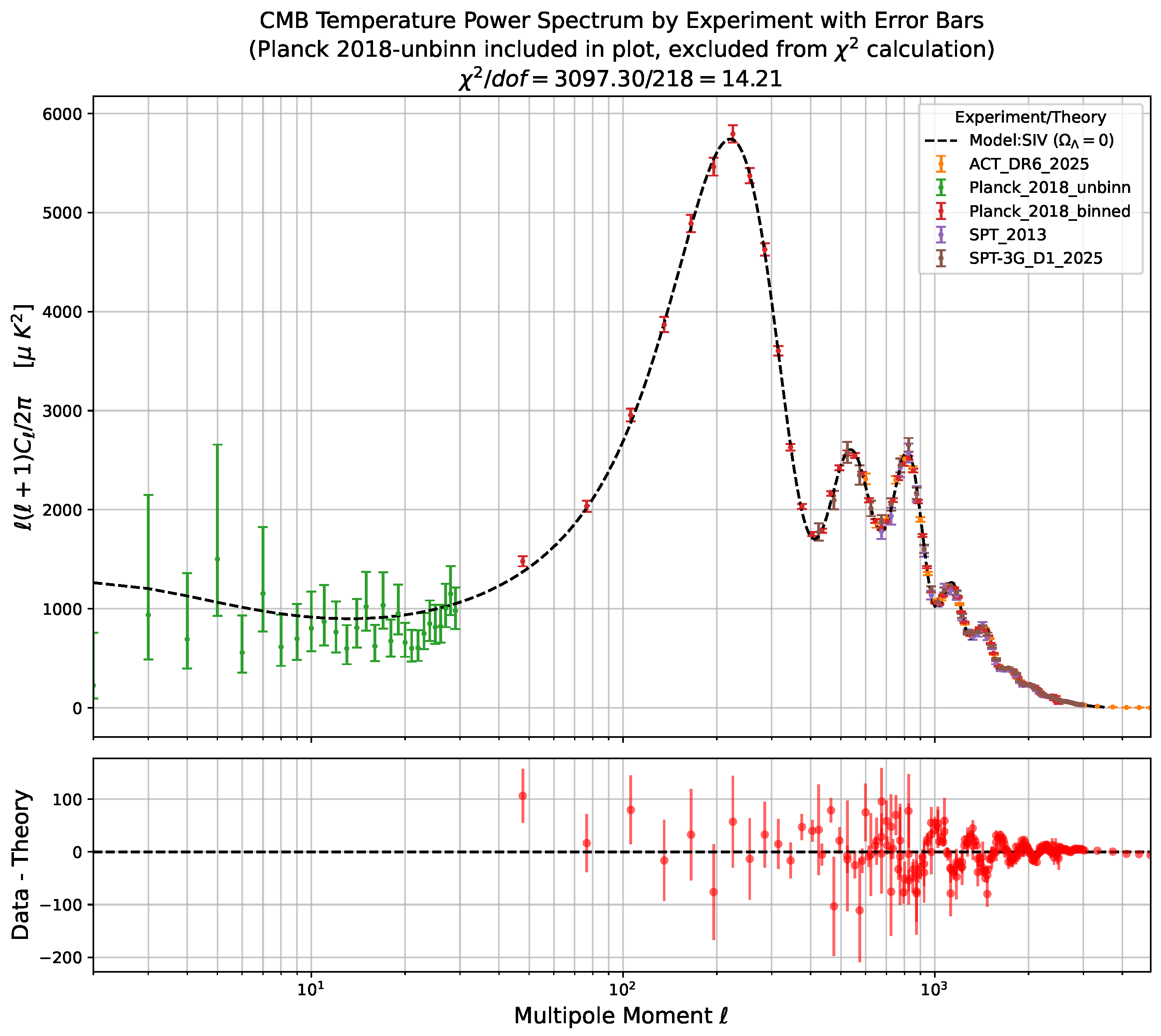
When the Hubble function is modified according to the discussion leading to (8) and (). The differences between and are very hard to be demonstrated graphically since is very small deviation from 1. As a result, having in the early universe, at radiation-matter equilibrium epoch and during decoupling implies that most of the other CMB properties such as TE/EE spectra, CMB lensing, and BAO should be reproduced as well while broader late-time expansion history will be guaranteed by the correct local . Upon using one observes shift of the CMB spectra to the right of the original un-modified standard LCDM spectra, then by adjusting only h from to the graph moves back to the left and almost overlaps with the original CMB spectra that traditionally predicts km/s/Mpc but now the results in km/s/Mpc instead. Starting with CMBQuick by using a consecutive search along each of the seven main cosmological parameters, , and SIV and h demonstrated U-shape landscape for each one; this way a set of adjusted cosmological parameters can be found and now the difference from the original LCDM CMB spectra is mostly less than a few percents. Finally, these parameters were used as a starting point for Pawell search method utilizing CASSy. As it can be seen in Figure 2 the difference from the LCDM is less then a present for most of . The corresponding CMB TT-spectra is shown in Figure 3 . The new model /dof=16.9 when the value for the LCDM is , while for the EE-spectra (not shown) the value is 6.64 for both, and for the TE-spectra (not shown) they are 9.06 and 9.25. Not shown here, but the results for the EE and TE spectra agree well with observation and MCMC type runs are now in progress too.
While there is a growing body of data, LCDM is still the simplest model that describes well the CMB. By finding alternative models that can do as well as LCDM by comparing -spectra guarantees such models to be well positioned to compete with LCDM. The calculation presents arrives at such cosmological parameters only by comparing but then the result is compared to other data sets found in the [24]. The original data sets indicated in this study on Figure 3 are: Planck 2018 [25] ACT DR6 2025 [26] SPT-3GD1 2025 [27] SPTpol 2017 [28] BICEP2/Keck 2015 [29]. Modern data processing is elaborate in how to add various data sets and how to estimate systematic and foreground errors [30]. Here I use the data to visualize how the theory compares to observation, the model parameters are derived by minimizing the deviation from the LCDM that results in a few percent differences Figure 2 . In particular, the specific datasets used for visualization here are hosted at the NASA LAMBDA archive as sources for the figures presented there. That is, the TT power spectrum plot data sources at [24]. For more context on the historical measurements and data sets see [31].
5. Discussion and Conclusions
The presented resolution of the Hubble tension does not require any new physics or fields, just a minor adjustment to the time parametrization due to the difference in gravitational potential that influences the length of the second over the evolution of the universe. As one would expect, higher energy density in the early universe results in increasing towards the past with respect to the current time t, as seen from the correspondence to from Figure 1.
Thus, according to (6), is well justified and the value of during the recombination is supported by the ration computed from the output of the CLASSy as sown in Figure 1. All of these supports the idea that the difference in gravitational potential, as seen from their ratios, is causing the Hubble tension as seen in (7).
Furthermore, unlike SIV where one cannot explain the meaning of , RISS clearly points to the difference between proper time and conformal time and the violation of their usual relation, according to (6) and utilizes a process as described to Section for testing and implementing the idea. That is, unlike the SIV theory prescribes a specific form , the RISS paradigm is more relaxed about the choice of that can pave the way towards determining the value of the cosmological constant and the phenomenon of dark matter as outlined in [10,11,12]. As such it will requires the development of specialized codes if the research is to fully comply with the SIV framework. However, here an alternative RISS approach of using has been utilized, based on the discussion in Section 3 and the derivation of the a-dependent rescaling of into ().
The present formalism has been implemented and visualized in Figure 3 and has resulted in resolution of the Hubble tension as demonstrated and explained in the previous sections. That is, as previously discussed in Section 2 epoch-dependent units rescaling symmetry has been already demonstrated. The effect of Weyl type time-reparametrization followed by its inverse epoch-dependent units rescaling affects only the time derivatives of a: that is, only H as defined by (10), but not its dependent relation (). Thus, the use of at the background level propagates to the corresponding background dynamics, perturbation treatment and observables remain consistent since the rescaling factor remains close to one near the epoch of decoupling.
In conclusion, the main idea presented here is that the discrepancy between the CMB-inferred and locally measured values of can be understood without introducing new particles or fields, but rather through a reinterpretation of the rate of change of the time variable entering the cosmological description as influenced by the differences in the overall gravitational potential during the decoupling and the current epoch.
Data Availability Statement
There are no new data associated with this article. However, the data underlying this article will be shared upon reasonable request to the corresponding author. The datasets used in this study could be provided by the corresponding author from one of the following platforms: GitHub repo, Kaggle dataset, or shared Google Drive upon reasonable request.
Acknowledgments
This research did not receive any specific grant from funding agencies in the public, commercial, or not-for-profit sectors. The author is grateful to his wife and daughters for their understanding and family support during the various stages of the research presented, and to Prof. Andre Maeder for the many years of fruitful and joyful explorations of the SIV paradigm.
Appendix A. Supplementary Materials
This supplementary sections for the paper includes:
CMB Related Equations
CMB Observables
Scale Invariant Cosmology
Figures A1 and A2
Time-Dependent Units
Appendix CMB Related Equations
Appendix CMB Observables
The photon source function [8] is given by
where is the photon visibility function, while is the photon monopole (intrinsic temperature), and are the gravitational potentials (metric perturbations), baryon velocity. Here is the Sachs-Wolfe effect, then Doppler terms , the last term describes the Integrated Sachs-Wolfe effect modulated by the exponential function of the optical depth . Upon adding polarization terms one has [13]:
Everything is in conformal time, thus invariant upon constant rescaling when integrated with . The co-moving distance is related to the conformal time that is used in the photon transfer function calculations with Bessel functions:
Appendix Scale Invariant Cosmology
The idea of Scale Invariant Cosmology has been discussed by Eddington, Dirac, Canuto et al, and further pushed by Buvie and Maeder [14,32,33,34] within the context of cosmology and astrophysics. The theory is often and easily mistaken for some type of Jordan-Brain-Dike conformal theory due to the absence of clear delimitation of what is the physical meaning of the conformal factor , which within SIV is taken to be dependent only on time due to homogeneity of space [9,10]. The corresponding FLRW equations for flat (corresponding to zero with ) have the form:
The above equations can be derived from the standard FLRW equations either by time-dependent time rescaling and/(or only) rescaling of the expansion scale factor . The rescaling is coming from the Weyl transformations of the metric since enters the Einstein equations via or via Weyl transformations as discussed earlier where rescaling by comes from the time rescaling along with to induce space rescaling. For constant one arrives back at the standard FLRW equations for the expansion scale factor and the Hubble function , for flat, homogeneous, and isotropic universe in the presence of a cosmological constant . In this case, there are usually only two equations - one related to energy-density balance and another related to the rate of change of H and the pressure content of the Universe:
By using , these equations can be written in an alternative form:
Furthermore, by considering different substances with equation of state , where for radiation one has , for matter and for the Einstein cosmological constant with . Then can be part of the energy density and pressure .
Notably, in the spirit of how the cosmological constant can be identified as substance with positive energy-density by inspecting (A12) and (). While the term may be identified also as substance but with a negative energy-density. Similarly, by inspection of (A9) and () , 3 can be related to negative energy-density but with ; now is a time-dependent substance because of , and is substance. However, let’s not take this route for now but instead let us look at what happens upon the symmetry transformations discussed earlier within the SIV gauge choice. The SIV choice of removes the corresponding and terms from the equations and therefore restores the scale invariance of the cosmological equations. Thus, determines via the SIV equations:
Appendix Figures A1 and A2
Figure A1.
The graphs depict the TT-spectra for with y-axis in units of and l on the x-axis. The solid blue line is the standard best LCDM model with corresponding to the Planck , the dashed green is the run using with that results in and the for transformation. The dotted red curve is using but with corresponding to the Local . The bottom shows the deviation of the doted red curve from the blue LCDM curve.
Figure A1.
The graphs depict the TT-spectra for with y-axis in units of and l on the x-axis. The solid blue line is the standard best LCDM model with corresponding to the Planck , the dashed green is the run using with that results in and the for transformation. The dotted red curve is using but with corresponding to the Local . The bottom shows the deviation of the doted red curve from the blue LCDM curve.
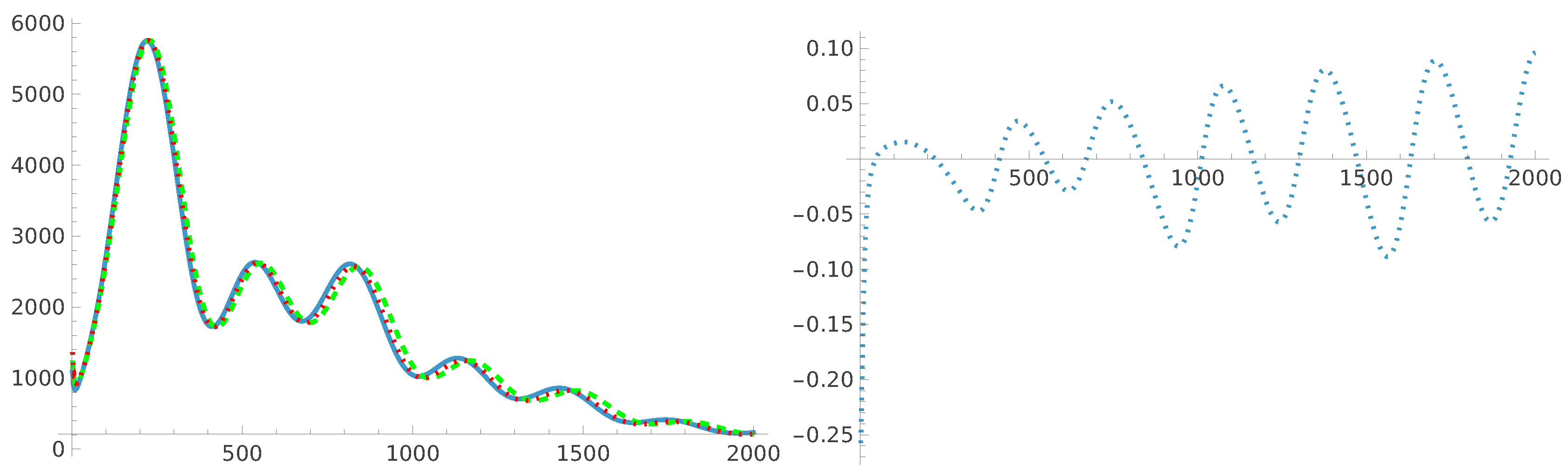
Figure A2.
The top graph shows the a-dependence of the “SIV” time t, , and the H scaling factor based on (8); that is, that results in and the for transformation. The bottom graph shows the deviation utilizing the adjusted cosmological parameters, that were fitted using to get close to the standard LCDM TT-spectra for ; the x-axis is l as usual. The new cosmology parameters that reproduce the LCDM TT-spectra for within less than a few percent for individual are and . The model parameter results in and for the transformation.
Figure A2.
The top graph shows the a-dependence of the “SIV” time t, , and the H scaling factor based on (8); that is, that results in and the for transformation. The bottom graph shows the deviation utilizing the adjusted cosmological parameters, that were fitted using to get close to the standard LCDM TT-spectra for ; the x-axis is l as usual. The new cosmology parameters that reproduce the LCDM TT-spectra for within less than a few percent for individual are and . The model parameter results in and for the transformation.
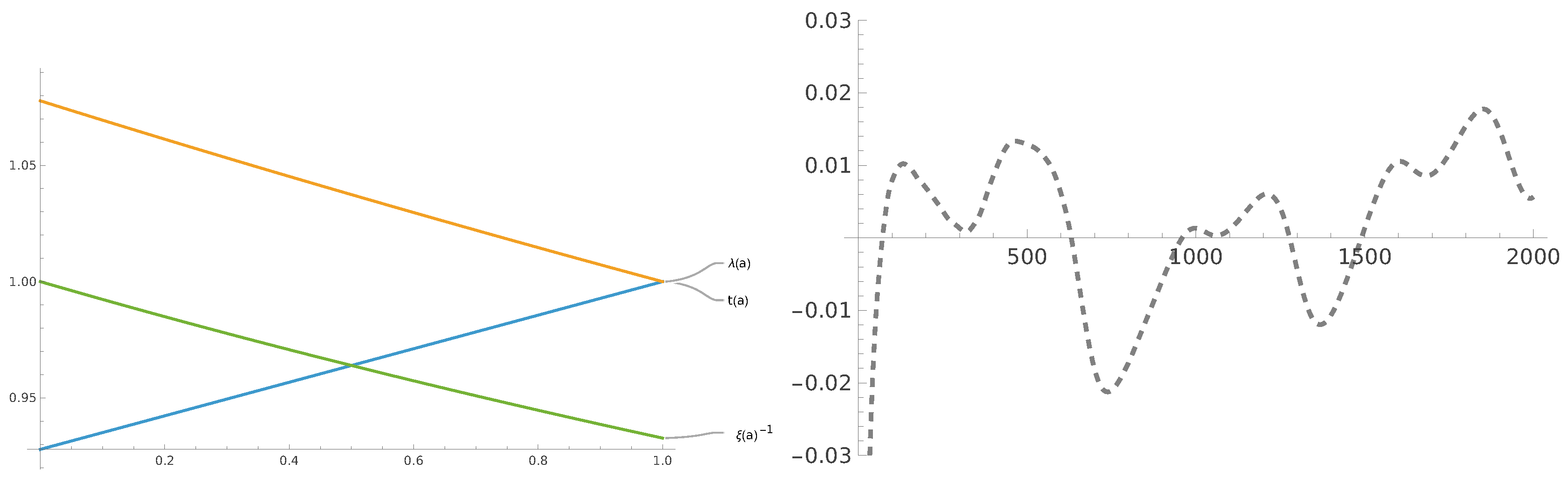
Appendix Time-Dependent Units
The above considerations brings us to the rules for how affects space and time () but does not tells us anything about energy. So one still has a freedom to choose the unit of energy. There are at least three possibilities: (1) one can fix the unit of mass using etalon just as it has been done in the past with the old unit of kilogram. In modern days it may be done using electron mass by measuring the mass to charge ratio of the electron; (2) one can adopt the modern definition of kilogram using fixed value for ℏ just as it is done for the unit of distance by using fixed value of the speed of light; (3) another alternative is to keep the Newton’s gravitational constant G fixed. The Scale Invariant Vacuum (SIV) gauge is taking this approach. One way to justify such choice is that within EGR constant G and c imply constant value of the cosmological constant which is the appropriate choice for studying large scale cosmological processes. When this is done, masses and the constant ℏ are subject to change by a factor , () but since at such scales, except for processes related to quantum gravity, then one can neglect A process where ℏ is important but is irrelevant is the BBN. This has been shown in recent study pointing to potential resolution of the primordial lithium-7 problem that indicates partially broken SIV symmetry in favor of the more adequate RISS paradigm [11,12,18]. Unlike SIV where a specific expression for is derived that guarantees constant , RISS does not have a definite functional form for but allows for alternatives depending on the process to be studied.
References
- Kamionkowski, M.; Riess, A.G. The Hubble Tension and Early Dark Energy. Annu. Rev. Nucl. Part. Sci. 2023, arXiv:astro73, 153–180. [Google Scholar] [CrossRef]
- Tdcosmo Collaboration; Birrer, S.; Buckley-Geer, E.J.; Cappellari, M.; Courbin, F.; Dux, F.; Fassnacht, C.D.; Frieman, J.A.; Galan, A.; Gilman, D.; et al. TDCOSMO 2025: Cosmological constraints from strong lensing time delays. Astron. Astrophys. 2025, arXiv:astro704, A63. [Google Scholar] [CrossRef]
- Abdalla, E.; Abellán, G.F.; Aboubrahim, A.; Agnello, A.; Akarsu, Ö.; Akrami, Y.; Alestas, G.; Aloni, D.; Amendola, L.; Anchordoqui, L.A.; et al. Cosmology intertwined: A review of the particle physics, astrophysics, and cosmology associated with the cosmological tensions and anomalies. J. High Energy Astrophys. 2022, arXiv:astro34, 49–211. [Google Scholar] [CrossRef]
- Wang, B.; López-Corredoira, M.; Wei, J.J. The Hubble tension survey: A statistical analysis of the 2012-2022 measurements. Mon. Not. R. Astron. Soc. 2024, arXiv:astro527, 7692–7700. [Google Scholar] [CrossRef]
- Courbin, F.; Maeder, A. The Hubble Tension in Light of the Symmetry of Scale Invariance. Symmetry 2026, 18. [Google Scholar] [CrossRef]
- Cyr-Racine, F.Y.; Ge, F.; Knox, L. Symmetry of Cosmological Observables, a Mirror World Dark Sector, and the Hubble Constant. Phys. Rev. Lett. 2022, arXiv:astro128, 201301. [Google Scholar] [CrossRef]
- Ge, F.; Cyr-Racine, F.Y.; Knox, L. Scaling transformations and the origins of light relics constraints from cosmic microwave background observations. Phys. Rev. D. 2023, arXiv:astro107, 023517. [Google Scholar] [CrossRef]
- Greene, K.L.; Cyr-Racine, F.Y. Thomson scattering: one rate to rule them all. J. Cosmol. Astropart. Phys. 2023, arXiv:astro2023, 065. [Google Scholar] [CrossRef]
- Maeder, A. An Alternative to the ΛCDM Model: The Case of Scale Invariance. Astrophys. J. 2017, arXiv:astro834, 194. [Google Scholar] [CrossRef]
- Gueorguiev, V.G.; Maeder, A. Elucidating the Dark Energy and Dark Matter Phenomena Within the Scale-Invariant Vacuum (SIV) Paradigm. Universe 2025, arXiv:astro11, 48. [Google Scholar] [CrossRef]
- Gueorguiev, V.G. Reparametrization Invariant Scaling Symmetry and the Value of the Einstein Cosmological Constant ΛE. In Proceedings of the Journal of Physics Conference Series. IOP; Journal of Physics Conference Series; 2024; Vol. 2910, p. 012014. [Google Scholar] [CrossRef]
- Gueorguiev, V.G. Reparametrization Invariance and Its Relation to the Dark Matter Phenomenon. In Proceedings of the Journal of Physics Conference Series. IOP; Journal of Physics Conference Series; 2025; Vol. 3002, p. 012003. [Google Scholar] [CrossRef]
- Tarsitano, F.; Schmitt, U.; Refregier, A.; Fluri, J.; Sgier, R.; Nicola, A.; Herbel, J.; Amara, A.; Kacprzak, T.; Heisenberg, L. Predicting cosmological observables with PyCosmo. Astron. Comput. 2021, 36, 100484. [Google Scholar] [CrossRef]
- Eddington, A.S. The mathematical theory of relativity, 2nd edition ed.; Cambridge University Press, 1923; p. 284. [Google Scholar]
- Dirac, P.A.M. Long Range Forces and Broken Symmetries. Proc. R. Soc. Lond. Ser. A 1973, 333, 403–418. [Google Scholar] [CrossRef]
- Canuto, V.; Adams, P.J.; Hsieh, S.H.; Tsiang, E. Scale-covariant theory of gravitation and astrophysical applications. Phys. Rev. D. 1977, 16, 1643–1663. [Google Scholar] [CrossRef]
- Bouvier, P.; Maeder, A. Consistency of Weyl’s Geometry as a Framework for Gravitation. Astrophys. Space Sci. 1978, 54, 497–508. [Google Scholar] [CrossRef]
- Gueorguiev, V.G. Scale-invariant vacuum guided resolution of the 7Li BBN problem. Astron. Astrophys. 2025, arXiv:nucl702, L5. [Google Scholar] [CrossRef]
- Ma, C.P.; Bertschinger, E. Cosmological Perturbation Theory in the Synchronous and Conformal Newtonian Gauges. Astrophys. J. 1995, arXiv:astro455, 7. [Google Scholar] [CrossRef]
- Hu, W.; Dodelson, S. Cosmic Microwave Background Anisotropies. Annu. Rev. Astron. Astrophys. 2002, 40, 171–216, Available online: arXiv:astro-ph/astro-ph/0110414. [Google Scholar] [CrossRef]
- Hu, W. Lecture Notes on CMB Theory: From Nucleosynthesis to Recombination. arXiv 2008, arXiv:0802.3688. [Google Scholar] [CrossRef]
- Blas, D.; Lesgourgues, J.; Tram, T. The Cosmic Linear Anisotropy Solving System (CLASS). Part II: Approximation schemes. J. Cosmol. Astropart. Phys. 2011, arXiv:astro2011, 034. [Google Scholar] [CrossRef]
- Pitrou, C. CMBquick: Spectrum and Bispectrum of Cosmic Microwave Background (CMB). Astrophysics Source Code Library, record ascl:1109.009. 2011. Available online: https://www2.iap.fr/users/pitrou/cmbquick.htm.
- NASA LAMBDA Archive. TT Power Spectrum Plot Data Sources. 2026. [Google Scholar] [PubMed]
- Planck Collaboration; Aghanim, N.; Akrami, Y.; Ashdown, M.; Aumont, J.; Baccigalupi, C.; Ballardini, M.; Banday, A.J.; Barreiro, R.B.; Bartolo, N.; et al. Planck 2018 results. VI. Cosmological parameters. Astron. Astrophys. 2020, arXiv:astro641, A6. [Google Scholar] [CrossRef]
- Louis, T.; La Posta, A.; Atkins, Z.; Jense, H.T.; Abril-Cabezas, I.; Addison, G.E.; Ade, P.A.R.; Aiola, S.; Alford, T.; Alonso, D.; et al. The Atacama Cosmology Telescope: DR6 power spectra, likelihoods and ΛCDM parameters. J. Cosmol. Astropart. Phys. 2025, arXiv:astro2025, 062. [Google Scholar] [CrossRef]
- Camphuis, E.; Quan, W.; Balkenhol, L.; Khalife, A.R.; Ge, F.; Guidi, F.; Huang, N.; Lynch, G.P.; Omori, Y.; Trendafilova, C.; et al. SPT-3G D1: CMB temperature and polarization power spectra and cosmology from 2019 and 2020 observations of the SPT-3G main field. Phys. Rev. D. 2026, arXiv:astro113, 083504. [Google Scholar] [CrossRef]
- Henning, J.W.; Sayre, J.T.; Reichardt, C.L.; Ade, P.A.R.; Anderson, A.J.; Austermann, J.E.; Beall, J.A.; Bender, A.N.; Benson, B.A.; Bleem, L.E.; et al. Measurements of the Temperature and E-mode Polarization of the CMB from 500 Square Degrees of SPTpol Data. Astrophys. J. 2018, arXiv:astro852, 97. [Google Scholar] [CrossRef]
- BICEP2/Keck Collaboration; Planck Collaboration; Ade, P.A.R.; Aghanim, N.; Ahmed, Z.; Aikin, R.W.; Alexander, K.D.; Arnaud, M.; Aumont, J.; Baccigalupi, C.; et al. Joint Analysis of BICEP2/Keck Array and Planck Data. Phys. Rev. Lett. 2015, 114, 101301, Available online: arXiv:astro-ph.CO/1502.00612. [Google Scholar] [CrossRef]
- Jense, H.T.; Viña, M.; Calabrese, E.; Hill, J.C. Choice of Planck CMB likelihood in cosmological analyses. Phys. Rev. D. 2026, arXiv:astro113, 043551. [Google Scholar] [CrossRef]
- NASA LAMBDA Archive. Hubble Constant History. 2026. [Google Scholar] [CrossRef]
- Dirac, P.A.M. Long Range Forces and Broken Symmetries. Proc. R. Soc. Lond. Ser. A 1973, 333, 403–418. [Google Scholar] [CrossRef]
- Canuto, V.; Adams, P.J.; Hsieh, S.H.; Tsiang, E. Scale-covariant theory of gravitation and astrophysical applications. Phys. Rev. D. 1977, 16, 1643–1663. [Google Scholar] [CrossRef]
- Bouvier, P.; Maeder, A. Consistency of Weyl’s Geometry as a Framework for Gravitation. Astrophys. Space Sci. 1978, 54, 497–508. [Google Scholar] [CrossRef]
- Maeder, A.; Gueorguiev, V.G. Action Principle for Scale Invariance and Applications (Part I). Symmetry 2023, arXiv:math15, 1966. [Google Scholar] [CrossRef]
- Gueorguiev, V.G.; Maeder, A. The Scale-Invariant Vacuum Paradigm: Main Results and Current Progress Review (Part II). Symmetry 2024, arXiv:gr16, 657. [Google Scholar] [CrossRef]
| 1 | Here I deviate from the traditional use of in the SIV literature and use instead. |
| 2 | |
| 3 | Here the use of as the time component of the connexion vector is preferred instead of k to avoid confusion with the wave number k used in the CMB related equations related to various quantities (). |
Figure 1.
The ratios of during decoupling and current epoch . Values taken from CLASSy run for standard LCDM. The cosmology parameters used are . The above trends has been reproduced using the CMBquick as well.
Figure 1.
The ratios of during decoupling and current epoch . Values taken from CLASSy run for standard LCDM. The cosmology parameters used are . The above trends has been reproduced using the CMBquick as well.
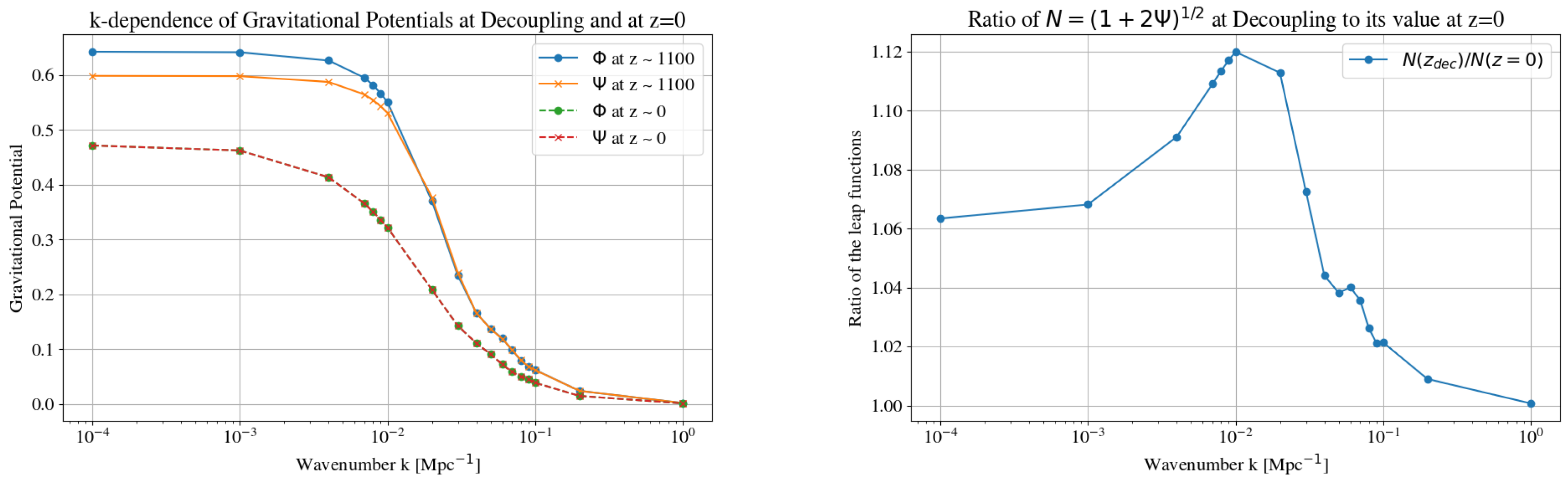
Figure 2.
The graph shows the deviation utilizing the adjusted cosmological parameters, that were fitted using to get close to the standard LCDM TT-spectra for ; the x-axis is l as usual. The new cosmology parameters that reproduce the LCDM TT-spectra for within less than a few percent for individual are and . The model parameter results in and for the transformation.
Figure 2.
The graph shows the deviation utilizing the adjusted cosmological parameters, that were fitted using to get close to the standard LCDM TT-spectra for ; the x-axis is l as usual. The new cosmology parameters that reproduce the LCDM TT-spectra for within less than a few percent for individual are and . The model parameter results in and for the transformation.
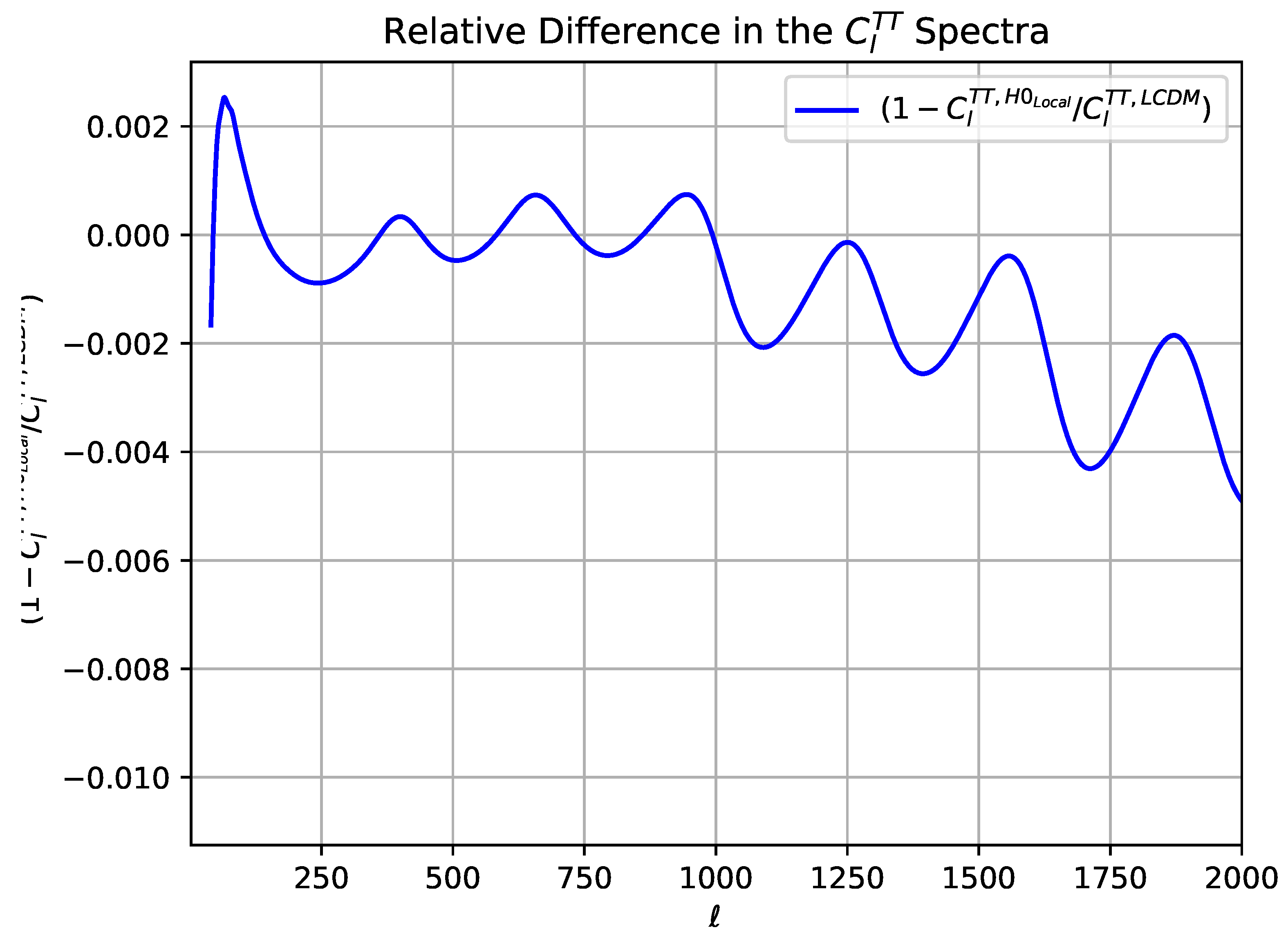
Figure 3.
Current model results as compared to the observational data on the CMB. Here . The is computed for the range of ℓ as shown on the graph but excludes the binned low-ℓ shown in green. The model /dof=14.21 compared to the value of for the LCDM, while for the EE-spectra (not shown) the value is 6.44 versus 6.64 for LCDM, and for the TE-spectra (not shown) is 9.25 for both.
Figure 3.
Current model results as compared to the observational data on the CMB. Here . The is computed for the range of ℓ as shown on the graph but excludes the binned low-ℓ shown in green. The model /dof=14.21 compared to the value of for the LCDM, while for the EE-spectra (not shown) the value is 6.44 versus 6.64 for LCDM, and for the TE-spectra (not shown) is 9.25 for both.
Disclaimer/Publisher’s Note: The statements, opinions and data contained in all publications are solely those of the individual author(s) and contributor(s) and not of MDPI and/or the editor(s). MDPI and/or the editor(s) disclaim responsibility for any injury to people or property resulting from any ideas, methods, instructions or products referred to in the content. |
© 2026 by the authors. Licensee MDPI, Basel, Switzerland. This article is an open access article distributed under the terms and conditions of the Creative Commons Attribution (CC BY) license (http://creativecommons.org/licenses/by/4.0/).
Copyright: This open access article is published under a Creative Commons CC BY 4.0 license, which permit the free download, distribution, and reuse, provided that the author and preprint are cited in any reuse.