

Submitted:
20 August 2026
Posted:
21 August 2026
You are already at the latest version
Abstract
The diffusion-time similarity transformation introduced by Sun [Phys. Fluids 36, 083616 (2024)] reduces the two-dimensional unsteady boundary layer equations to a single partial differential equation in the two variables η = y/δ(x) and τ = νt/δ2(x). We extend the reduction to an electrically conducting fluid at low magnetic Reynolds number and show that the reduced problem changes type. Grouping the time-derivative terms reveals that the coefficient of the highest mixed derivative is 1 − Λ with Λ = cτfη, so that a frozen-coefficient analysis gives the growth rate λ = −k2/(1 − Λ): marching forwards in the diffusion time is parabolic only where Λ < 1 and backward-parabolic beyond. For a power-law outer stream U = Cxm we find Λ = (1 − m)ut/x, so the threshold coincides with the Stewartson starting-front criterion t = x/u for a flat plate. Integrating the constancy conditions rather than postulating a profile shows that the admissible flows comprise exactly three families—power-law, exponential and uniform—the exponential one being missed by the usual ansatz. Constancy of the magnetic interaction parameter is a separate condition, B0δ = const, so a uniform applied field is admissible only where the layer does not grow—that is, only at a stagnation point. The reduction is unconditionally well posed for m ≥ 1 and, for m < 1, must be integrated backwards in τ beyond τ = 1/c, which corresponds to marching downstream. A second-order implicit scheme confirms the threshold sharply: for c = 2 the wall shear is grid-converged to six figures up to τ = 0.45 on four successive meshes and diverges non-monotonically in the mesh beyond τ = 0.5. We further derive the two-term strong-field expansion fηη(0) ≃ M1/2 + (a/12 + 2b/3)M−1/2 for the magnetic interaction parameter M, which reproduces published spectral benchmarks to eight significant figures and fixes the prefactor of the √M friction law at unity.
Keywords:
diffusion-time similarity transformation
; unsteady boundary-layer equations
; low magnetic Reynolds number
; Stewartson starting-front criterion
; magnetic interaction parameter
1. Introduction
The diffusion-time similarity transformation proposed by Sun [1] reduces the two-dimensional unsteady laminar boundary layer equations from three independent variables to two. Writing the stream function as with and , the streamwise coordinate is eliminated entirely provided the coefficients of the reduced equation are constant, and a single two-dimensional problem then describes the flow at every station. This is a partial reduction rather than a reduction to an ordinary differential equation: the symmetry algebra of the unsteady boundary layer equations, classified by Ma and Hui [2], is too small to permit the latter for a general outer stream. The construction has since been applied to conducting fluids by Fu, Ni and Zhang [3], who obtained closed-form approximations for stagnation and converging flows under a spanwise field.
The reduction raises a question that does not arise for the classical steady similarity variables, and that appears not to have been addressed. Because depends on x through , surfaces of constant are not in general transverse to the direction along which the parabolic boundary layer equations propagate information. One should therefore ask whether the reduced equation may be integrated as an initial-value problem in at all. We show below that it may not: the equation changes type at a critical value of that depends on the outer-flow exponent, and beyond that value forward marching is ill posed in the sense of Hadamard.
The threshold turns out to have a transparent physical meaning. For a power-law outer stream the parabolicity parameter reduces to , so that for a flat plate the reduced problem is well posed precisely in the region that has not yet been reached by the starting front propagating from the leading edge. This is the same region in which Stewartson’s small-time solution [4] holds, recovered here from the type of the transformed equation rather than from a matched asymptotic expansion. For accelerated outer flows, , the obstruction is absent and the march is unconditionally well posed; the stagnation-point case is distinguished twice over, since it is also the only case in which a spatially uniform applied magnetic field is compatible with similarity.
We work throughout with an electrically conducting fluid at low magnetic Reynolds number, , the regime relevant to liquid metals in ducts, moulds and fusion blankets [5,6]. The induced field is then negligible and the electromagnetic problem reduces to the quasi-static determination of the electric potential. The magnetic case is of interest here not only for its own sake but because the Lorentz force provides an independent control on the velocity profile: it alters , hence , hence the location of the threshold, and it supplies a second verification route through the strong-field asymptotics developed in Sec. Section 4.3.
The paper is organised as follows. Section 2 sets out the governing equations, the quasi-static closure of the Lorentz force, and the similarity reduction, together with the conditions under which the coefficients are constant. Section 3 contains the central result: the parabolicity condition, its physical interpretation, and the consequences for the marching direction. Section 4 collects the limiting solutions used for verification, including the two-term strong-field expansion. Section 5 describes the numerical scheme and its verification, and Sec. Section 6 reports the numerical test of the threshold and its physical consequences.
2. Formulation and Similarity Reduction
2.1. Governing Equations and the Lorentz Closure
Consider the two-dimensional unsteady flow of an incompressible, viscous, electrically conducting fluid past a plane wall, with a magnetic field applied normal to the wall (Figure 1). At low the current follows from Ohm’s law for a moving conductor, , with .
The force involves two successive cross products, and it is worth writing both out. The motional term is
so the wall-normal velocity does not contribute and the induced current is purely spanwise, . This spanwise current then crosses the wall-normal field a second time, and since , the force is directed along the wall:
A spanwise current in a wall-normal field therefore produces a streamwise force; this is the mechanism responsible for the Hartmann layer [16]. Note that the result depends on , so reversing the field direction, , leaves (2) unchanged once is reversed with it.
The value of in (2) is fixed by the electrical boundary conditions. Applying the outer-flow momentum balance at the edge of the layer,
shows that the short-circuited choice , which gives , is incompatible with a steady outer stream: with it requires . It is admissible only if the free stream is allowed to decay as , which destroys the separability the reduction requires. We therefore take , so that the current vanishes in the outer stream and
in agreement with the closure used by Chiam [7] and Parand et al. [8]. Under the boundary layer approximation the governing equations are then
with at , as , and an impulsive start for .
Remark 1
(Why a wall-normal field). The alternative orientation is a spanwise field , for which lies in the plane of the flow. The streamwise force is then , which for reduces to : thesameexpression as (4). The two orientations therefore give identical momentum equations, and differ only in the electrostatic problem that must be solved to obtain them.
That difference is the reason for the present choice. With the motional term (1) is purely spanwise, so in two dimensions holds identically: no potential is induced, and is fixed by the external circuit alone. With , by contrast, in general, ϕ must be obtained from a Poisson problem, and for an insulating wall the potential contributes a further half of the total force, doubling the effective coefficient [3]. The wall-normal orientation is thus the one for which the two-dimensional low- problem closes without an auxiliary electrostatic equation; all results below carry over to the spanwise case under .
2.2. The Diffusion-Time Transformation
Introducing the stream function , , Eqs. (5) and (6) collapse to
and we apply the transformation of Ref. [1],
The derivatives of the new variables are , , and , whence
Setting recovers the equation of Ref. [1], and the form (12) agrees with that of Ref. [3] under the correspondence . The boundary conditions become
Remark 2.
Had the short-circuited closure been used, the magnetic term in (12) would read . Evaluating the equation as , where and all derivatives vanish, then leaves the residual , so no solution satisfying (14) exists for . With (4) the same limit gives identically. This compatibility check is worth performing on any similarity formulation of a damped boundary layer.
2.3. Complete Determination of the Admissible Flows
Equation (12) is a genuine two-variable reduction if and only if a, b, c and M are independent of x. Rather than postulate a form for U and and verify constancy afterwards, we take constancy as the defining condition and integrate the resulting system, which determines the admissible flows completely.
Writing , the definitions (13) of b and c are two first-order ordinary differential equations for the pair ,
while a is not independent, since
The requirement is therefore simply that the Hartmann number formed with the local layer thickness be the same at every station; the applied field must scale inversely with the layer it damps. This statement is independent of the solution of (15) and holds for every case below.
Lemma 1
(Admissible outer flows). The system (15) with b, c constant admits exactly three families, distinguished by the value of .
(A) : power-law flows.Dividing the two equations of (15) gives , whence ; substituting back and integrating yields , that is
with and
Constancy of M then requires, by (17), .
(B) , : exponential flows.Here , , and , so that (15) gives and
with for constant M.
(C) : uniform flows.Then U and δ are both constant, , and is uniform. This is the degenerate case of Sec. Section 4.2.
Three points deserve emphasis. First, family (A) contains a virtual origin that the usual statement of the similarity conditions suppresses; it is a genuine free parameter, and for the flat plate (, U const) it appears as , the familiar leading-edge offset.
Second, family (B) is not a power law and is not reached by the ansatz , which degenerates when . It is nevertheless an exact similarity family: an exponentially accelerating outer stream over an exponentially thinning layer, with an exponentially strengthening field. Its coefficients satisfy identically, so by the criterion of Sec. Section 3 an accelerating member (, hence , ) is unconditionally well posed, while a decelerating one () is conditional. For this family the parabolicity parameter takes the particularly simple form .
Third, the residual freedom in K within family (A) is a gauge choice for , not additional physics. We fix it by the Falkner–Skan convention , so that
3. Change of Type and Well-Posedness
3.1. The Parabolicity Condition
The terms of (12) containing -derivatives may be grouped as
so that the coefficient multiplying the highest mixed derivative is not unity but , where
This single observation determines the character of the reduced problem.
Lemma 2
(Parabolicity condition). Let f solve (12) and consider a short-wave perturbation with at frozen coefficients. Retaining the highest derivative on each side, the principal balance is , whence
Forward evolution in τ is therefore parabolic and well posed where , and backward-parabolic—hence ill posed as an initial-value problem in increasing τ—where .
Because , with equality attained only in the free stream, the critical condition is met first, and simultaneously across the whole outer part of the layer, at
For , that is for , one has everywhere and the forward march is unconditionally well posed. Equation (24) also shows that the effective diffusivity in is , so that the approach to the threshold is accompanied by a progressive stiffening of the problem even before the type changes.
3.2. Physical Interpretation: The Starting Front
For a flat plate, , the condition is exactly : the reduction may be marched forwards in precisely in the region that has not yet been reached by the starting front propagating downstream from the leading edge. This is the classical criterion delimiting the validity of Stewartson’s small-time solution for the impulsively started plate [4], obtained here from the type of the transformed equation rather than from a matched asymptotic expansion. The last column of Table 1 lists for each case; decelerated flows reach the threshold sooner than the flat plate, and accelerated flows with never reach it. For the exponential family (B) of Lemma 1 the same parameter is , so that an accelerating exponential stream is well posed for all .
The magnetic field enters this criterion indirectly but not negligibly. Since the Lorentz force makes the profile fuller, raising at fixed , it raises throughout the layer and therefore brings the interior of the layer to the threshold earlier, even though itself, fixed by the free stream, is unchanged.
3.3. The Correct Marching Direction
The loss of well-posedness for is not a defect of the reduction but a statement about the direction in which information travels. At fixed t, decreasing corresponds to increasing x. The region is therefore the already-established region near the leading edge, and there the boundary layer equations are parabolic in x with the marching direction downstream, that is, towards decreasing . The properly posed formulation for and is thus a terminal-value problem, integrated backwards in from the steady Falkner–Skan state at , and (24) with gives decay rather than growth in that direction. Attempting instead to march forwards through produces the grid-dependent divergence documented in Sec. Section 6.
Two consequences follow. First, any statement about the transient of a decelerated or zero-pressure-gradient layer obtained by forward marching in beyond is not supported by the equation. Second, the stagnation-point case is the natural setting for unsteady computations within this framework, being both unconditionally well posed and compatible with a uniform applied field.
3.4. Relation to the Group-Theoretic Classification
It is worth locating this obstruction within the Lie-group classification of similarity reductions of the unsteady boundary layer equations given by Ma and Hui [2]. Their analysis shows that the symmetry algebra of the unsteady equations admits only a small number of families of invariant solutions, distinguished by the dependence of the free stream on x and t; it is too small to reduce the general problem to an ordinary differential equation. The transformation (8) is a partial reduction that sidesteps this by eliminating x at the cost of constraining U and . The obstruction identified above is the further, and to our knowledge previously unremarked, price of that construction: because depends on x, the level surfaces of cross the characteristic surfaces of the original parabolic system, and the reduced problem inherits a change of type at the crossing. A characterisation of this obstruction directly in terms of the characteristic surfaces of the unreduced system would be a natural extension of Ref. [2].
4. Limiting Solutions
Three limits of (12) admit closed-form or classical results. The first two are known and are recorded here because they supply the initial condition and the verification cases for the numerical scheme; the third is derived below and appears to be new.
4.1. Steady Limit
4.2. Small-Time Limit
As the physical layer thickness is much smaller than , so , and are , while , and are all . The leading balance is
which is exact for all in the degenerate case . With and this is subject to , , , whose solution is the MHD Rayleigh–Stokes profile of Chang and Yen [15],
with wall shear
4.3. Strong-Field Expansion
For the velocity defect is confined to a Hartmann layer of thickness . Introducing and with , Eq. (27) becomes
At leading order with , , giving
Writing and ,
whose bounded solution with is
Since , the wall shear is
and the integral thicknesses satisfy , , so that the shape factor tends to the value of a purely exponential profile,
Equation (35) confirms the friction scaling reported in Ref. [3] and fixes its prefactor: the leading coefficient is exactly unity in the present normalisation, whereas the closed-form estimate of Ref. [3] gives . The discrepancy originates in the near-wall Taylor truncation of and used there, which preserves the exponent but not the coefficient. The accuracy of (35) is assessed against independent spectral data in Sec. Section 6.
5. Numerical Method and Verification
The steady problem (27) is solved by fourth-order collocation with residual-based mesh adaptation, tolerance , and truncation length ; selected cases were reproduced by shooting with an eighth-order Runge–Kutta integrator and a secant iteration on , the two agreeing to twelve significant figures for . For the scheme returns for the flat plate and for plane stagnation flow, and the separation eigenvalue , reproducing the classical values [11,13] to better than .
For the unsteady problem we take as the primary unknown on a uniform grid , , recovering f by cumulative trapezoidal quadrature. Since the solution spans several decades of , we march in , so that and (12) reads
Spatial derivatives use second-order central differences and the BDF2 formula, with implicit Euler on the first step. The quadratic term is treated by Newton linearisation and the non-local couplings through f and by Picard iteration, so each iterate requires only a tridiagonal solve; iteration stops when successive iterates differ by less than , typically after three to six sweeps. The scheme is fully implicit and imposes no stability restriction on within the well-posed region —a point of some importance for the test in Sec. Section 6, since it means that any divergence observed there cannot be attributed to a step-size restriction. The initial condition at is (29).
Three verification tests were performed. First, with the computed solution is compared with (29); Figure 2(a) shows the relative error in the wall shear for –25, below for and largest at the earliest times, where the layer thickness is resolved by only a few cells. Second, Table 2 and Figure 2(b) report a refinement study with spatial and temporal resolution varied independently; the observed spatial order is , , , over four refinements. Third, for the value of obtained by marching to agrees with the independently computed solution of (27) to at , at and at , the degradation reflecting the thinning of the Hartmann layer at fixed h.
6. Results
6.1. Test of the Strong-Field Expansion
Table 3 compares the computed wall shear with the independent spectral results of Ref. [8] and with the expansion (35), for a strongly decelerated () and an accelerated () outer flow. Agreement between the present computation and the published values is to seven or eight significant figures across four decades in M, which validates the solver; the interest here is the last two columns. The two-term expansion is accurate to already at and to better than at , and the convergence is consistent with the predicted remainder: between and at the relative error falls by a factor of 16, against the factor of 8 expected from the remainder alone and 32 from a naive estimate.
Figure 3 shows the accompanying prediction for the integral quantities. The wall shear follows and the displacement thickness , and the shape factor collapses onto from above, reaching at for every b examined. The last result gives a compact diagnostic: since H is bounded below by 2 and takes values near for Blasius flow, the departure of H from 2 measures how far the magnetic field is from having taken over the momentum balance entirely.
6.2. Numerical Test of the Parabolicity Threshold
Table 4 and Figure 4 test Lemma 2 directly. For the flat plate, and (25) predicts . On four successive meshes spanning a factor of eight in h, the computed wall shear at , and agrees to six significant figures, with differences decreasing as ; the solution below the threshold is thus fully grid-converged.
Beyond the behaviour changes qualitatively. The computed values diverge, and—this is the essential point—they diverge differently on each mesh, non-monotonically in N: at the four grids return , , and . Refinement does not restore convergence, and the coarsest grid is not the worst. This is precisely what (24) predicts for : the amplification rate is proportional to and hence unbounded as , so the outcome is governed by whatever short-wave content the particular mesh admits. Because the scheme is fully implicit, the divergence cannot be attributed to a time-step restriction.
Figure 4(b) shows the complementary case. For , 2 and 3, all of which have , the march proceeds smoothly over five decades in and converges to the respective steady values. The short-time behaviour is common to all cases, as it must be, since as irrespective of the sign of c; the histories separate only once .
6.3. The Unconditionally Well-Posed Case
For the reduction is well posed for all , and the complete transient may be computed. Figure 5 shows the evolution from the Rayleigh–Stokes state to the steady MHD stagnation-point profile: at the computed profile is indistinguishable from (29), and by the steady state has essentially been attained.
Figure 6(a) shows that at small all wall-shear histories collapse onto the field-free Rayleigh singularity , since the magnetic term is while the diffusive terms are ; the field is felt only once . Thereafter each curve relaxes to its own plateau. Defining the relaxation time as the value of beyond which remains within of its steady value, we obtain
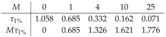
The product tends to a constant near , so that at strong field: the magnetic damping time replaces the viscous diffusion time as the controlling timescale, and the field accelerates the approach to the steady state as well as altering the state itself.
Figure 6(c) shows the shape factor. Every case starts from the value of the error-function profile, independently of M, and relaxes monotonically to its steady value— at , at , at —approaching the limit (36). The monotonicity indicates that the profile becomes fuller throughout the transient, with no intermediate overshoot.
7. Conclusions
We have extended the diffusion-time similarity reduction of Sun [1] to the unsteady boundary layer of a conducting fluid at low magnetic Reynolds number and examined the type of the reduced equation. The main conclusions are the following.
The reduced problem changes type. Grouping the time-derivative terms shows that the coefficient of the highest mixed derivative is with , and a frozen-coefficient analysis gives the growth rate . Forward marching in the diffusion time is therefore well posed only where , and for the threshold is reached at .
The threshold is the starting front. For a power-law outer stream , so the condition is, for a flat plate, exactly . The restriction on the reduction thus coincides with the classical criterion delimiting Stewartson’s small-time solution, recovered here from the type of the equation rather than from a matched expansion. Since decreasing corresponds to increasing x, the correct formulation beyond the threshold is a terminal-value problem integrated backwards in , which is downstream marching.
Numerical experiment confirms the threshold sharply. For the wall shear is grid-converged to six figures up to on four meshes and diverges non-monotonically in the mesh beyond , over eighty orders of magnitude, despite a fully implicit scheme. For () the march is unconditionally stable, and the stagnation-point case is doubly distinguished, being also the only case compatible with a uniform applied field.
A two-term strong-field expansion, , reproduces independent spectral benchmarks to eight significant figures and fixes the prefactor of the friction law at unity, in place of the obtained in Ref. [3] from a near-wall truncation. In the same limit and , and the relaxation time of the transient scales as .
Finally, a formulation point of general applicability: the quasi-static Lorentz force must be closed as if the outer stream is steady, so that it enters the reduced equation as . The alternative closure leaves a residual in the free stream and admits no solution satisfying (Remark 2).
Two extensions suggest themselves. The first is to solve the terminal-value problem for and so close the flat-plate transient within the similarity framework, which would permit a direct quantitative comparison with Stewartson’s matched asymptotic solution across . The second is to characterise the change of type directly in terms of the characteristic surfaces of the unreduced system, within the group-theoretic setting of Ref. [2].
References
- Sun, B. H. Similarity solutions of a class of unsteady laminar boundary layer. Phys. Fluids 2024, 36, 083616. [Google Scholar] [CrossRef]
- Ma, P. K. H.; Hui, W. H. Similarity solutions of the two-dimensional unsteady boundary-layer equations. J. Fluid Mech. 1990, 216, 537–559. [Google Scholar] [CrossRef]
- Fu, J.-Y.; Ni, M.-J.; Zhang, N.-M. Theoretical analysis for non-linear effects of magnetic fields on unsteady boundary layer flows. arXiv 2025, arXiv:2504.06576. [Google Scholar]
- Stewartson, K. On the impulsive motion of a flat plate in a viscous fluid. Q. J. Mech. Appl. Math. 1951, 4, 182–198. [Google Scholar] [CrossRef]
- P. A. Davidson, An Introduction to Magnetohydrodynamics; Cambridge University Press: Cambridge, 2001.
- Müller, U.; Bühler, L. Magnetofluiddynamics in Channels and Containers; Springer: Berlin, 2001. [Google Scholar]
- Chiam, T. C. Hydromagnetic flow over a surface stretching with a power-law velocity. Int. J. Eng. Sci. 1995, 33, 429–435. [Google Scholar] [CrossRef]
- Parand, K.; Rezaei, A. R.; Ghaderi, S. M. An approximate solution of the MHD Falkner–Skan flow by Hermite functions pseudospectral method. Commun. Nonlinear Sci. Numer. Simul. 2011, 16, 274–283. [Google Scholar] [CrossRef]
- Abbasbandy, S.; Hayat, T. Solution of the MHD Falkner–Skan flow by homotopy analysis method. Commun. Nonlinear Sci. Numer. Simul. 2009, 14, 3591–3598. [Google Scholar] [CrossRef]
- Falkner, V. M.; Skan, S. W. Some approximate solutions of the boundary layer equations. Philos. Mag. 1931, 12, 865–896. [Google Scholar] [CrossRef]
- Hartree, D. R. On an equation occurring in Falkner and Skan’s approximate treatment of the equations of the boundary layer. Proc. Camb. Philos. Soc. 1937, 33, 223–239. [Google Scholar] [CrossRef]
- Stewartson, K. Further solutions of the Falkner–Skan equation. Proc. Camb. Philos. Soc. 1954, 50, 454–465. [Google Scholar] [CrossRef]
- Smith, A. M. O. Improved solutions of the Falkner and Skan boundary-layer equation. J. Aeronaut. Sci. 1954, 21, 1–18. [Google Scholar]
- Asaithambi, N. S. A numerical method for the solution of the Falkner–Skan equation. Appl. Math. Comput. 1997, 81, 259–264. [Google Scholar] [CrossRef]
- Chang, C. C.; Yen, J. T. Rayleigh’s problem in magnetohydrodynamics. Phys. Fluids 1959, 2, 393–403. [Google Scholar] [CrossRef]
- Hartmann, J. Hg-dynamics I: Theory of the laminar flow of an electrically conductive liquid in a homogeneous magnetic field. K. Dan. Vidensk. Selsk. Mat. Fys. Medd. 1937, 15(6), 1–28. [Google Scholar]
- Rossow, V. J. On flow of electrically conducting fluids over a flat plate in the presence of a transverse magnetic field. NACA Report 1358. 1958.
- Riley, N. Unsteady laminar boundary layers. SIAM Rev. 1975, 17, 274–297. [Google Scholar] [CrossRef]
- D. P. Telionis, Unsteady Viscous Flows; Springer: New York, 1981.
- Schlichting, H.; Gersten, K. Boundary-Layer Theory, 9th ed.; Springer: Berlin, 2017. [Google Scholar]
- Takhar, H. S.; Nath, G. Similarity solution of unsteady boundary layer equations with a magnetic field. Meccanica 1997, 32, 157–163. [Google Scholar] [CrossRef]
- Fang, T. G.; Wang, F. J.; Gao, B. Unsteady magnetohydrodynamic stagnation point flow—closed-form analytical solutions. Appl. Math. Mech. 2019, 40, 449–464. [Google Scholar] [CrossRef]
Figure 1.
Configuration. A power-law outer stream flows over a plane wall in the presence of a wall-normal magnetic field with . The induced current (circle, directed out of the page) crosses to give a streamwise Lorentz force opposing the motion of the fluid relative to the free stream.
Figure 1.
Configuration. A power-law outer stream flows over a plane wall in the presence of a wall-normal magnetic field with . The induced current (circle, directed out of the page) crosses to give a streamwise Lorentz force opposing the motion of the fluid relative to the free stream.
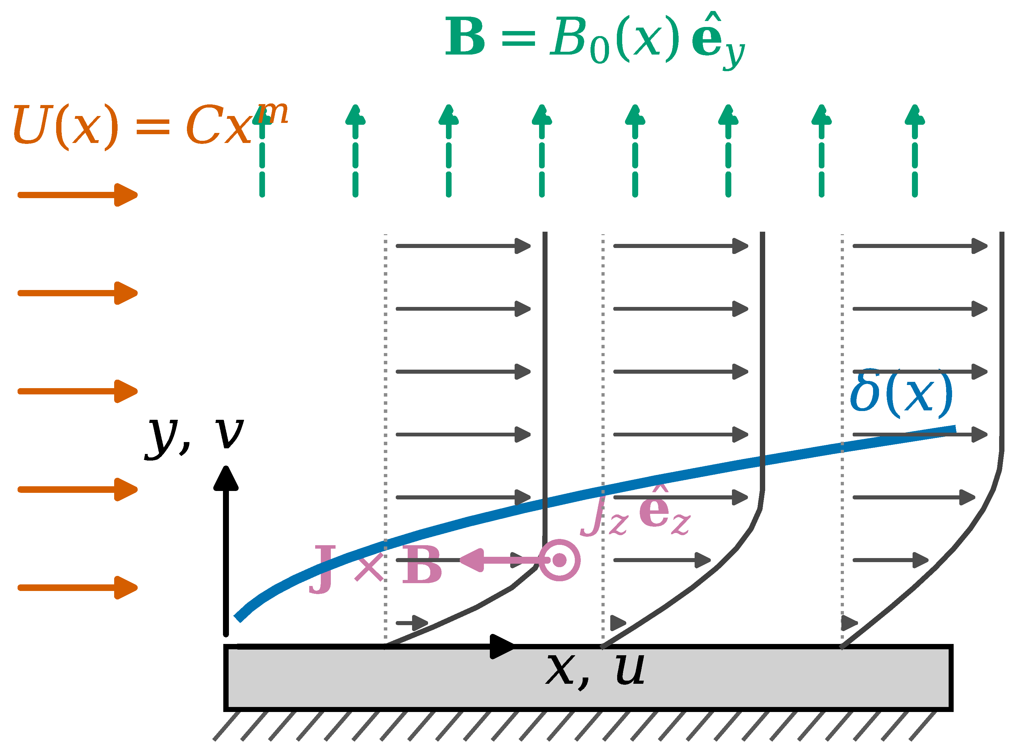
Figure 2.
Verification of the unsteady solver. (a) Relative error of the computed wall shear with respect to the exact result (30) for . (b) Independent spatial and temporal refinement at , ; both sequences follow the second-order reference slope until the temporal errors reach the spatial error floor.
Figure 2.
Verification of the unsteady solver. (a) Relative error of the computed wall shear with respect to the exact result (30) for . (b) Independent spatial and temporal refinement at , ; both sequences follow the second-order reference slope until the temporal errors reach the spatial error floor.
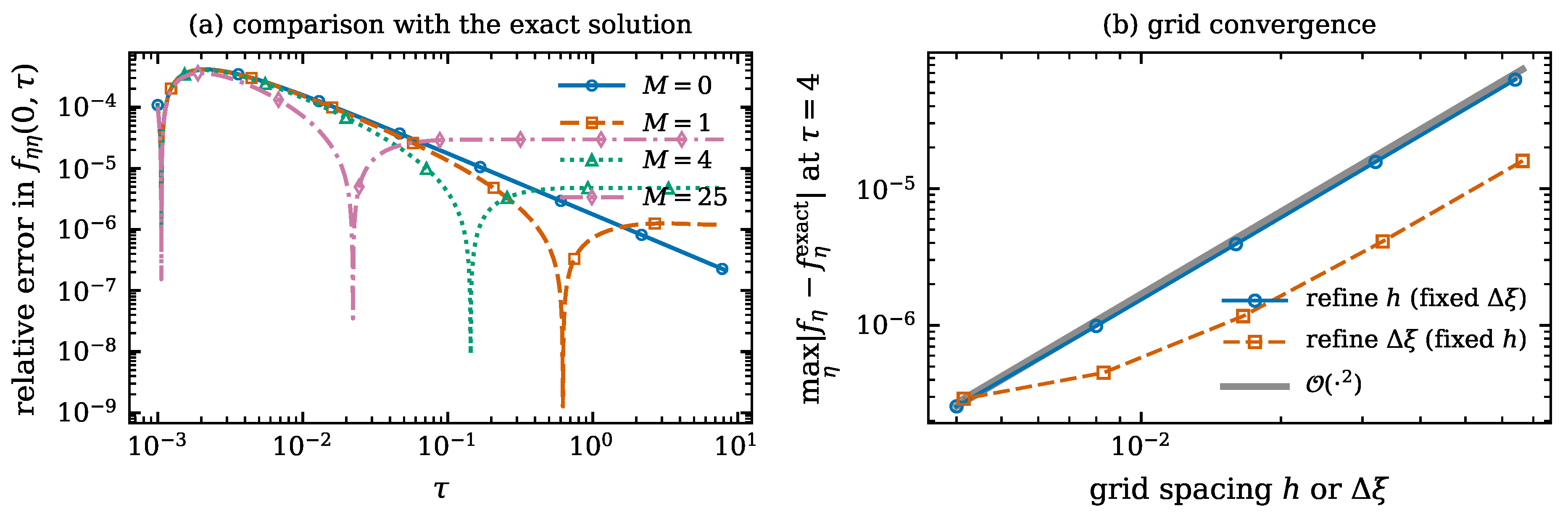
Figure 3.
Global steady quantities against M for several pressure-gradient parameters b, tested against the strong-field expansion of Sec. Section 4.3. (a) Wall shear, approaching ; (b) displacement thickness, approaching ; (c) shape factor, approaching the value of Eq. (36).
Figure 3.
Global steady quantities against M for several pressure-gradient parameters b, tested against the strong-field expansion of Sec. Section 4.3. (a) Wall shear, approaching ; (b) displacement thickness, approaching ; (c) shape factor, approaching the value of Eq. (36).
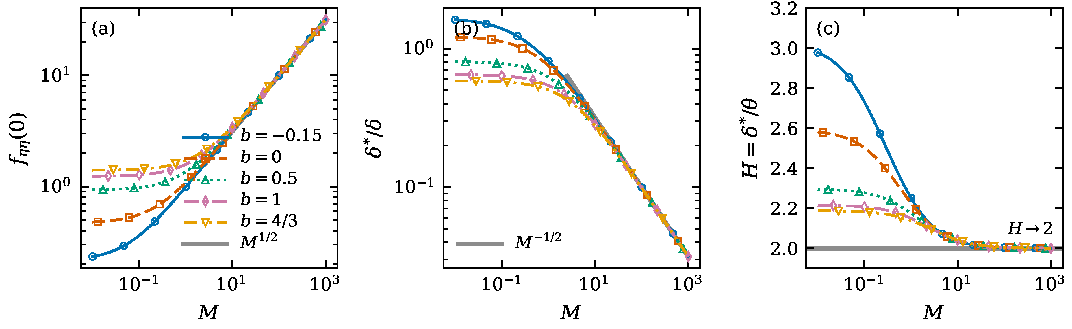
Figure 4.
(a) Forward marching for a flat plate (, ) on three grids. The curves are indistinguishable for and diverge beyond it, with an onset and growth rate that depend on the mesh. (b) Wall-shear histories at for several m; the cases () march to the steady state without difficulty, whereas the case can be continued only to .
Figure 4.
(a) Forward marching for a flat plate (, ) on three grids. The curves are indistinguishable for and diverge beyond it, with an onset and growth rate that depend on the mesh. (b) Wall-shear histories at for several m; the cases () march to the steady state without difficulty, whereas the case can be continued only to .
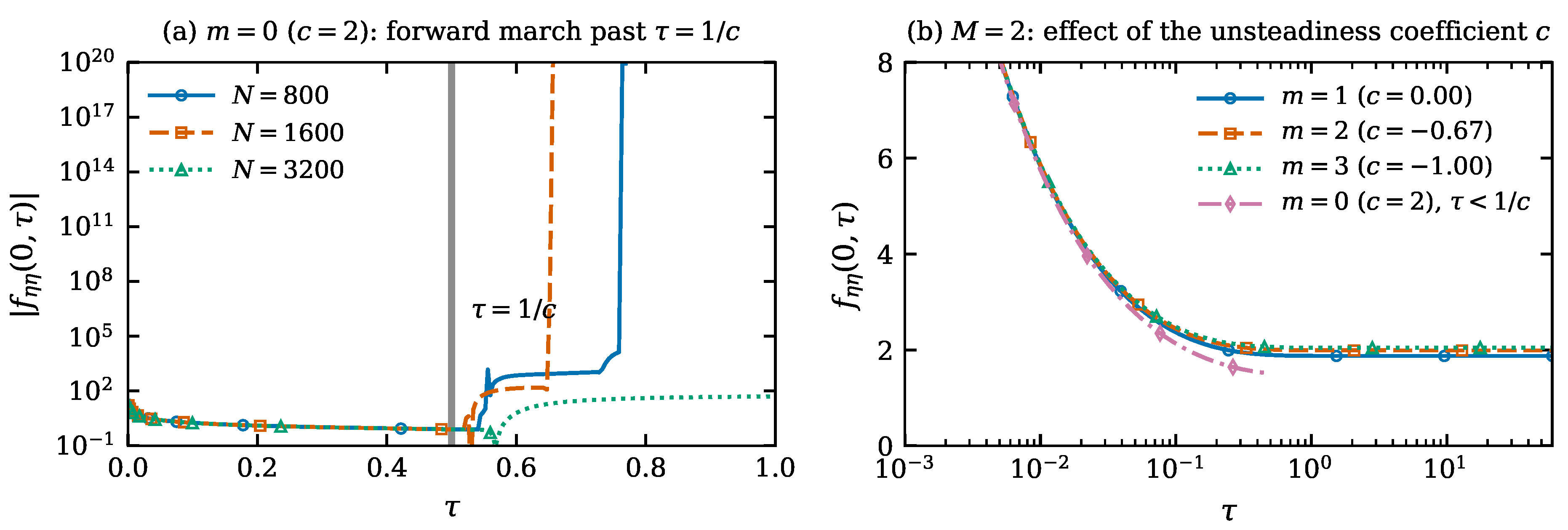
Figure 5.
Evolution of the velocity profile for plane stagnation-point flow (, , ) at (a) and (b) . The grey dashed curve is the exact small-time profile (29) at ; the heavy grey curve is the steady solution of (27). Every curve is identified by colour, dash pattern and marker together, so that all panels remain legible in monochrome.
Figure 5.
Evolution of the velocity profile for plane stagnation-point flow (, , ) at (a) and (b) . The grey dashed curve is the exact small-time profile (29) at ; the heavy grey curve is the steady solution of (27). Every curve is identified by colour, dash pattern and marker together, so that all panels remain legible in monochrome.
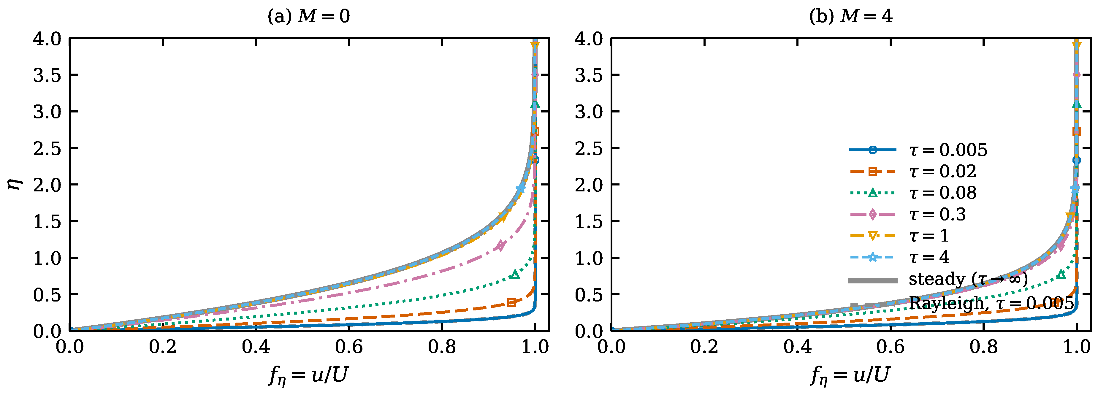
Figure 6.
Unsteady stagnation-point flow (, ). (a) Wall shear against diffusion time; the two heavy grey curves are the exact small-time solution (30) for and . (b) Wall shear normalised by its steady value. (c) Shape factor, starting from the Rayleigh value and relaxing to the steady value.
Figure 6.
Unsteady stagnation-point flow (, ). (a) Wall shear against diffusion time; the two heavy grey curves are the exact small-time solution (30) for and . (b) Wall shear normalised by its steady value. (c) Shape factor, starting from the Rayleigh value and relaxing to the steady value.
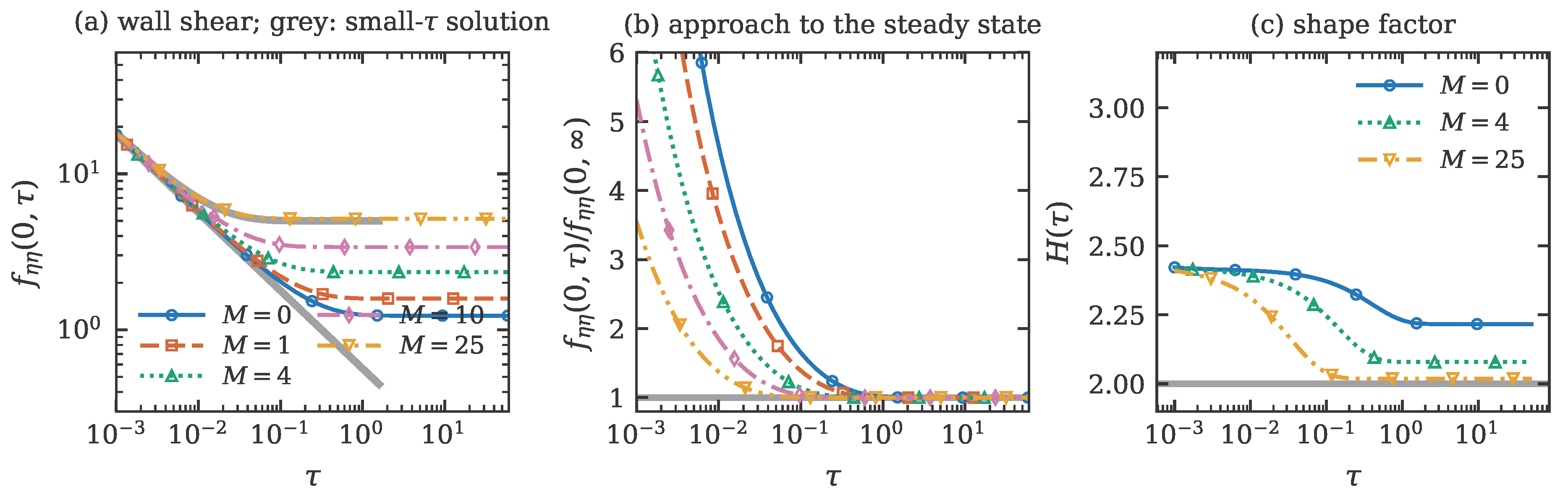

Table 1.
Similarity coefficients in the gauge (21) () for representative outer flows, with the field distribution required for constant M and the character of the forward -march established in Sec. Section 3. The threshold applies when . Upper block: power-law family (A) of Lemma 1, for which ; the first row is incipient separation of the non-magnetic layer. Lower block: exponential family (B), for which .
Table 1.
Similarity coefficients in the gauge (21) () for representative outer flows, with the field distribution required for constant M and the character of the forward -march established in Sec. Section 3. The threshold applies when . Upper block: power-law family (A) of Lemma 1, for which ; the first row is incipient separation of the non-magnetic layer. Lower block: exponential family (B), for which .
| flow | m | b | c | type of -march | ||
|---|---|---|---|---|---|---|
| decelerated wedge | conditional | |||||
| flat plate | 0 | 0 | 2 | conditional | ||
| wedge, | conditional | |||||
| wedge, | 1 | conditional | ||||
| plane stagnation point | 1 | 1 | 0 | const | unconditional | — |
| accelerated | 2 | unconditional | — | |||
| accelerated | 3 | x | unconditional | — | ||
| family (B): , , | ||||||
| accelerating | — | unconditional | — | |||
| decelerating | — | conditional | ||||
Table 2.
Grid convergence of the unsteady solver against the exact solution (29) with and , measured as at . Spatial and temporal resolution are refined independently; the temporal sequence saturates once it reaches the spatial error floor of .
Table 2.
Grid convergence of the unsteady solver against the exact solution (29) with and , measured as at . Spatial and temporal resolution are refined independently; the temporal sequence saturates once it reaches the spatial error floor of .
| spatial refinement (4000 steps in ) | temporal refinement () | |||||
|---|---|---|---|---|---|---|
| h | error | order | error | order | ||
| 0.064 | — | 0.0664 | — | |||
| 0.032 | 2.00 | 0.0332 | 1.95 | |||
| 0.016 | 2.00 | 0.0166 | 1.82 | |||
| 0.008 | 1.99 | 0.0083 | 1.38 | |||
| 0.004 | 1.95 | 0.0041 | 0.63 | |||
Table 3.
Wall shear of the MHD Falkner–Skan equation compared with the Hermite pseudospectral results of Parand et al. [8] and the finite-difference values of Asaithambi [14] (their parameter satisfies ), together with the two-term expansion (35) and its relative error.
| M | present | Ref. [8] | Eq. (35) | rel. error of (35) | |
|---|---|---|---|---|---|
| , | |||||
| 5 | 25 | 4.60075228 | 4.60075494 | 4.6166667 | |
| 10 | 100 | 9.80646300 | 9.80646420 | 9.8083333 | |
| 15 | 225 | 14.87167401 | 14.87167484 | 14.8722222 | |
| 20 | 400 | 19.90393626 | 19.90393701 | 19.9041667 | |
| 50 | 2500 | 49.96165198 | 49.96165233 | 49.9616667 | |
| , | |||||
| 5 | 25 | 5.19095980 | 5.19095945 | 5.1944444 | |
| 10 | 100 | 10.09677575 | 10.09677545 | 10.0972222 | |
| 50 | 2500 | 50.01944084 | 50.01944071 | 50.0194444 | |
| 100 | 10000 | 100.00972177 | 100.00972170 | 100.0097222 | |
Table 4.
Forward -marching for a flat plate (, , , ), for which Lemma 2 predicts . Below the threshold the wall shear is grid-converged to six figures; above it the computed values are not merely inaccurate but vary non-monotonically over eighty orders of magnitude as the mesh is refined, which is the signature of an ill-posed problem rather than of discretisation error. All runs use and 1000 steps in .
Table 4.
Forward -marching for a flat plate (, , , ), for which Lemma 2 predicts . Below the threshold the wall shear is grid-converged to six figures; above it the computed values are not merely inaccurate but vary non-monotonically over eighty orders of magnitude as the mesh is refined, which is the signature of an ill-posed problem rather than of discretisation error. All runs use and 1000 steps in .
| : | : | |||||
|---|---|---|---|---|---|---|
| N | h | |||||
| 800 | 0.01750 | 1.261691 | 0.953711 | 0.841087 | ||
| 1600 | 0.00875 | 1.261598 | 0.953669 | 0.841058 | ||
| 3200 | 0.00438 | 1.261574 | 0.953658 | 0.841050 | ||
| 6400 | 0.00219 | 1.261568 | 0.953656 | 0.841048 | ||
Disclaimer/Publisher’s Note: The statements, opinions and data contained in all publications are solely those of the individual author(s) and contributor(s) and not of MDPI and/or the editor(s). MDPI and/or the editor(s) disclaim responsibility for any injury to people or property resulting from any ideas, methods, instructions or products referred to in the content. |
© 2026 by the authors. Licensee MDPI, Basel, Switzerland. This article is an open access article distributed under the terms and conditions of the Creative Commons Attribution (CC BY) license (http://creativecommons.org/licenses/by/4.0/).
Copyright: This open access article is published under a Creative Commons CC BY 4.0 license, which permit the free download, distribution, and reuse, provided that the author and preprint are cited in any reuse.