

Submitted:
20 August 2026
Posted:
20 August 2026
You are already at the latest version
Abstract
Tropical Amazonian forests serve as critical carbon reservoirs, although their storage capacity varies significantly depending on the topographic, hydrologic, and successional heterogeneity of the landscape. This study quantified aboveground biomass (AGB) and carbon stocks across four vegetation units in the Tacshitea sector, Sierra del Divisor Na-tional Park (Peru): semi-dense flooded forest (Z1), hill forest (Z2), hill forest associated with secondary growth (Z3), and Mauritia flexuosa palm forest (Z4). We established 100 plots of 20 × 20 m (1 ha per zone), assessing all individuals with diameter at breast height (DBH) ≥ 10 cm using allometric equations validated for Amazonian ecosystems. A total of 2,363 individuals belonging to 158 species from 41 families were recorded. AGB varied sig-nificantly among vegetation units (Kruskal-Wallis, p < 0.001), with the highest values in Z1 (414.09 Mg ha⁻¹; 194.62 Mg C ha⁻¹) and Z2 (332.01 Mg ha⁻¹; 156.05 Mg C ha⁻¹), whereas Z3 and Z4 recorded substantially lower values (145.27–153.18 Mg ha⁻¹; 68.28–71.99 Mg C ha⁻¹). The Fabaceae family dominated carbon storage at the landscape scale (33.82%). Floristic diversity showed positive but weak associations with carbon storage (R² = 0.045–0.056), and this relationship lost significance when controlling for spatial structure using linear mixed-effects models (p = 0.409), indicating that structural attributes—particularly basal area and wood density—are more robust predictors of storage capacity than taxo-nomic richness per se. Beta diversity analysis revealed that floristic differentiation among zones was dominated by species turnover, explaining 26.5% of the variation by vege-tation unit (PERMANOVA, F = 11.55; p = 0.001). These results support the relevance of Sierra del Divisor National Park as a priority carbon sink in the western Peruvian Amazon and underscore the necessity of conservation strategies that integrate the structural heterogeneity of the forest mosaic.
Keywords:
biomass estimation
; carbon sequestration
; non-destructive sampling
; western Amazonia
; wood density
1. Introduction
Tropical forests, which cover 7–10% of Earth's land surface, represent the biome with the highest primary productivity and regulate the major biogeochemical cycles [1]. These ecosystems function as important carbon reservoirs, storing approximately 25% of terrestrial carbon in their aboveground and belowground biomass and soil horizons [2]. Furthermore, they contribute to climate system regulation through annual sequestration of 1.0–1.4 peta-grams of carbon, which attenuates global warming [3]. However, the Amazon basin shows progressive weakening in its carbon sink capacity, associated with increased tree mortality linked to climatic anomalies and landscape fragmentation, compromising ecosystem resilience [4].
Sierra del Divisor National Park (SDNP) stands as the third most extensive protected area in Peruvian Amazonia, encompassing 1,354,485 hectares distributed across the regions of Ucayali and Loreto [5]. Its volcanic mountain massifs exceed 900 meters, constituting the headwaters of ten major river basins [6]. The landscape hydrology of these ecosystems delineates seasonally inundated territories encompassing blackwater floodplain systems (tahuampas) associated with adjacent mountainous massifs, as well as extensive peatland networks characterized by organic substrates undergoing slow decomposition that exceed 5 m in depth, functioning as substantial belowground carbon reservoirs [5,7]. The pronounced topographic and hydrological heterogeneity inherent to these systems drives marked spatial variability in canopy structure and wood density — two critical biophysical attributes that directly govern the distribution of aboveground biomass across landscape scales [8].
Understanding variation in biomass storage capacity is fundamental, given that forest ecosystems span a continuum of successional states shaped by both natural landscape heterogeneity and post-disturbance regeneration dynamics. These processes collectively determine the structural complexity of forest stands and their capacity to accumulate and retain carbon over time [9]. In this context, empirically derived allometric models represent the methodological standard for estimating aboveground biomass at the individual tree level, offering a non-destructive approach that preserves stand structural integrity while enabling robust carbon quantification across ecologically diverse forest types [10,11].
To evaluate the role of the SDNP in the global carbon cycle this study quantified aboveground biomass and carbon stocks across four structurally distinct vegetation units within the Tacshitea sector, employing non-destructive allometric methods. Three working hypotheses were formulated to guide the analysis: (H1) aboveground biomass and carbon stocks differ significantly among vegetation units, with hill forests exhibiting greater storage capacity attributable to their higher structural complexity; (H2) hill forests associated with secondary successional dynamics present lower carbon density relative to mature forests, reflecting differences in stand development stage; and (H3) floristic diversity and canopy structural attributes are positively associated with aboveground biomass and carbon storage capacity across vegetation units.
2. Materials and Methods
2.1. Study Area
Sierra del Divisor National Park (SDNP), established in 2015, encompasses 1,354,485 ha in the departments of Ucayali and Loreto. It was created to protect a representative sample of the steep mountain region within the Amazonian humid tropical forest, with elevations near 1,000 m.a.s.l. This hill system, of volcanic origin, harbors a complex network of river basins that drain toward the Ucayali River in Peru and the Yuruá River in Brazil [5,12]. Among its principal functions are the protection of biological, geomorphological, and cultural diversity of indigenous peoples in situations of isolation and initial contact (PIACI), such as the Isconahua, Mayoruna, and Kapanawa peoples.
SDNP plays a key role in transboundary ecological connectivity, integrating a binational biological corridor of more than three million hectares [5]. Geologically, it constitutes one of the oldest formations in Amazonia, with landscapes of high geomorphological heterogeneity and difficult access, which has favored ecological integrity [13] and the presence of endemic and restricted-distribution species [14].
According to Holdridge's (1947) classification [15], SDNP corresponds to Tropical Humid Forest (bh-T), with annual precipitation of 1,600–2,000 mm, seasonality between October and April, and mean temperature of 25 °C [16,17].
Fieldwork was conducted between March and October 2025 at the Tacshitea Control and Surveillance Post (PCP) (7°53'54.39"S, 74°29'55.68"W; Figure 1), located on the banks of the river of the same name, a water body that potentially contributes to floristic differentiation patterns in western Amazonia [18,19]. Authorized anthropogenic activities in the area are restricted to scientific research and controlled ecotourism, safeguarding the subsistence rights of local communities [5].
2.2. Field Sampling
One hundred plots of 20 × 20 m (0.04 ha each) were established and distributed across four sampling zones in the Tacshitea sector (25 plots per zone; 1 ha sampled per zone), representative of the environmental heterogeneity of the area: semi-dense flooded forest (Z1), hill forest (Z2), hill forest associated with secondary growth (Z3), and palm forest dominated by Mauritia flexuosa (Z4). Selection was based on their physiographic, hydrological, floristic, and structural differences.
Plots were established with a minimum spacing of 40 m between them to reduce local spatial dependence, and zones were separated by at least 1,200 m. Biomass, carbon, and structural attribute values are presented standardized per hectare to facilitate comparisons; however, plots should be interpreted as spatial subsamples within each vegetation unit, not as independent geographical replicates. Therefore, statistical comparisons describe differences among the evaluated units in the Tacshitea sector and are not intended to be extrapolated to the entire SDNP.
The four zones encompass a gradient of ecological conditions, successional states, and hydrological regimes (Figure 2). Z1 (blackwater floodplain) and Z4 (palm swamp) correspond to hydromorphic systems with recurrent flooding; Z2 is a mature terra firme formation; and Z3 represents a secondary forest whose original disturbance is associated with subsistence agriculture (cassava, plantain, citrus) abandoned approximately ten years before sampling, allowing evaluation of structural recovery and post-disturbance carbon accumulation. Low recent human intervention in Z1 and Z4 is partly due to their difficult accessibility and flooding regime.
In each plot, all tree, shrub, and palm individuals with DBH ≥ 10 cm were evaluated, recording DBH and total height estimated with a SUUNTO clinometer [20]. Botanical samples were collected for taxonomic identification by a specialist using specialized literature and comparison with herbarium specimens [21]. Nomenclature was standardized with Plants of the World Online (POWO; https://powo.science.kew.org) and family classification followed the Angiosperm Phylogeny Website (APG; https://www.mobot.org/mobot/research/apweb/).
2.3. Calculation of AGB and Carbon Stock
To quantify aboveground biomass (AGB) and estimate carbon stocks, an empirical methodological approach based on dendrometric dimensions was followed using allometric equations validated for Amazonian ecosystems.
For each tree individual, basal area (BA) was calculated from diameter at breast height (DBH) using the following equation:
BA = (π × DBH²)/4000
Wood volume (V) was estimated by integrating basal area, total height (H), and a form factor of 0.7, according to the methodology proposed by Brown (1997) [22]:
V = BA × H × 0.7
Aboveground biomass (AGB) of woody plants was calculated by multiplying volume by wood-specific gravity (ρ), diameter at breast height (DBH), and total height (H) [10]:
AGB = (0.0673 * (ρ * (DBH²) * H) ^0.976)/1000
Wood density (ρ) for each taxon was assigned using the Global Wood Density Database [23].
For AGB estimation in palms (family Arecaceae), specific allometric models developed by Goodman et al. (2013) were applied [24].
Total carbon content was estimated by multiplying total aboveground biomass (Mg) by a carbon conversion factor (CF) of 0.47, as recommended by the IPCC [25] for tropical forests. Results were expressed as carbon stocks (Mg ha⁻¹).
2.4. Data Analysis
Forest structure was characterized by using descriptive statistics (mean ± SD) at the plot level. To evaluate differences among vegetation units, the Kruskal-Wallis test was employed, given that data did not meet the assumptions of normality (Shapiro-Wilk) or homogeneity of variances (Levene), followed by pairwise comparisons using Dunn's post-hoc test with Bonferroni correction. Results should be interpreted as comparisons among the units evaluated in the Tacshitea sector, without extrapolation to the entire SDNP. Basal area, aboveground biomass, and carbon values were expressed per hectare (1 ha sampled per zone).
Vertical stratification was evaluated using the Pretzsch index, a modification of the Shannon index applied to altitudinal structure. Individuals were classified into three strata according to the maximum height recorded per zone (Figure 3): upper (80–100%), middle (50–80%), and lower (0–50%) [26,27].
Floristic composition was assessed using the Importance Value Index (IVI) [28]. Alpha diversity was estimated using Shannon's (H′), Simpson's (1 − D), Pielou's evenness (J′), Fisher's α, and Margalef (DMg) indices. Species richness was compared among zones using rarefaction curves and abundance-based interpolation/extrapolation (q = 0). Asymptotic richness was estimated with Chao1, and sampling completeness was calculated as the ratio of observed to estimated richness using the iNEXT package [29].
Beta diversity was quantified using Bray–Curtis, Jaccard, and Sørensen indices. Sørensen dissimilarity was partitioned into turnover (Simpson dissimilarity) and nestedness components following Baselga (2010) [30] using the betapart package [31]. A SIMPER analysis [32] identified the species contributing most to compositional dissimilarity among zone pairs. All analyses and figures were produced in R v4.6.0 [33] using the tidyverse [34], vegan [35], iNEXT, betapart, and dunn.test packages.
3. Results
3.1. Floristic Composition and Diversity
3.1.1. Floristic Composition and Importance Value Index (IVI)
Global IVI identified Inga edulis as the species with the highest relative importance (25.9), followed by Jacaranda copaia (17.3), Ocotea obovata (15.4), Bauhinia brachycalyx (13.9), Pouteria caimito (13.4), and Aniba hostmanniana (12.9), concentrating the highest values among the 20 taxa with the greatest IVI recorded (Figure 4).
IVI by zone revealed differences in dominant composition among sampling units (Figure 5). In Z1, Bauhinia brachycalyx dominated (34.93), followed by Dialium guianense (18.03) and Mauritia flexuosa (16.66). In Z2, Jacaranda copaia stood out (43.5), while in Z3 and Z4 the dominant species was Ocotea obovata (IVI = 31.52 and 40.51, respectively). Inga edulis ranked among the species with highest IVI in three zones: Z2 (36.7), Z3 (30.45), and Z4 (36.66).
3.1.2. Alpha Diversity
A total of 2,363 individuals (DBH ≥ 10 cm) belonging to 41 families and 158 species were recorded (Table 1). Z1 presented the highest richness (99 spp.), followed by Z3 (73), Z2 (59), and Z4 (39). The best-represented families were Fabaceae (35.5%), Lauraceae (25.6%), and Arecaceae (9.8%).
Alpha diversity indices showed differences among zones (Table 2). Z1 recorded the highest values for Shannon (H' = 3.636), Simpson (1-D = 0.946), Fisher (α = 34.492), and Margalef (DMg = 15.427), with 574 individuals. Z3 presented H' = 3.425 and 1-D = 0.939 (503 ind.); Z2, H' = 3.209 and 1-D = 0.938 (628 ind.); and Z4, despite concentrating the highest abundance (658 ind.), recorded the lowest diversity (H' = 2.759; 1-D = 0.903). Pielou's evenness (J') ranged between 0.753 (Z4) and 0.798 (Z3).
Rarefaction curves confirmed the gradient Z1 > Z3 > Z2 > Z4 (Figure 6). Chao1 estimators projected 133.7, 104.9, 68.8, and 45.1 species for Z1, Z3, Z2, and Z4, respectively. Sampling completeness was higher in Z4 (86.4%) and Z2 (85.7%), while Z1 (74.0%) and Z3 (69.6%) did not reach the asymptote by the end of the sampling effort.
3.1.3. Diversity and Floristic Differentiation
Baselga's (2010) [30] partitioning showed that floristic dissimilarity among zones was dominated by species turnover (Figure 7). The Z1–Z3(βSørensen ≈ 0.64) and Z1–Z4 (βSørensen ≈ 0.62) comparisons presented the highest values of total dissimilarity; in both cases turnover was the predominant component, although Z1–Z4 also showed a contribution from nestedness. The Z3–Z4 comparison recorded the lowest total dissimilarity and the highest relative contribution of nestednes.
Classic indices confirmed the marked floristic differentiation (Table 3), with Z1–Z3 being the most dissimilar pair (Jaccard = 0.7801; Bray-Curtis = 0.7493; Sørensen = 0.6395) and Z3–Z4 the most similar (Bray-Curtis = 0.6546; Jaccard = 0.4933; Sørensen = 0.6607).
SIMPER analysis (Figure 8) identified Ocotea obovata, Bauhinia brachycalyx, Inga edulis, Cecropia engleriana, Jacaranda copaia, and Mauritia flexuosa as the species with greatest contribution to floristic differences among zones. In comparisons with Z1, Jacaranda copaia and Bauhinia brachycalyx stood out; in comparisons with Z4, Ocotea obovata; and in Z3–Z4 the contributions were distributed without marked dominance.
PERMANOVA (Bray-Curtis) revealed significant differences in floristic composition among zones (F = 11.55; R² = 0.265; p = 0.001; Table 4). PERMDISP revealed heterogeneity in multivariate dispersion (F = 16.68; p = 0.001), attributable mainly to Z4, whose dispersion differed significantly from the other zones (p < 0.001), while Z1, Z2, and Z3 showed no differences among themselves (Appendix 2).
NMDS ordination (Bray-Curtis; stress = 0.271) showed partial separation of plots by zone (Figure 9). Although the stress value indicates limited two-dimensional representation, the pattern is consistent with compositional differences detected by PERMANOVA.
3.2. Forest Structure
3.2.1. Vertical Structure and Stratification
The Pretzsch index evidenced dominance of the lower stratum (0–50% of maximum height) in all zones (Figure 10; Kruskal-Wallis, p < 0.05). Z2 concentrated the highest proportion in this stratum (85.4%, N = 536; mean height = 15.5 ± 5.7 m), followed by Z1 (78.7%, N = 452; 11.9 ± 3.9 m).
In the middle stratum (50–80%), Z4 showed the highest representation (24.5%, N = 161; 20.7 ± 2.7 m), followed by Z3 (23.5%, N = 118; 21.4 ± 2.7 m). Z2 had the lowest participation at this level (14.3%, N = 90), although with individuals up to 39.5 m, evidencing marked discontinuity toward the canopy.
The upper stratum (80–100%) was underrepresented in all zones. Z2 recorded the lowest incidence (0.3%, N = 2) but the highest height values (51.5 ± 2.1 m; maximum 53 m). Z3 retained the highest relative proportion in the canopy (4.4%, N = 22; 30.2 ± 2.6 m), with more balanced structural dynamics. Mean heights in the lower stratum of Z3 (11.6 m) and Z4 (11.7 m) indicate more homogeneous regeneration structure compared to the vertical heterogeneity of Z1 and Z2.
Dunn's post-hoc tests (Table 5) revealed significant differences among zones in all three strata. For height, comparisons Z1–Z3 and Z1–Z4 (p < 0.001) stood out in the upper stratum. In the middle and lower strata, most comparisons for richness and abundance were significant (p < 0.05), particularly those involving Z3. Collectively, these results indicate differentiated vertical distribution among the four zones, with contrasting patterns in the composition of each stratum (Table 5).
3.2.2. Diameter and Height Distribution
Diameter distribution showed the inverted J pattern in all four zones, with the highest concentration in the 10–20 cm class (53.5–67.0% of total; Figure 11). In Z3 and Z4, more than 90% of individuals had DBH < 30 cm, while Z1 and Z2 showed greater representation in middle and high classes, including individuals > 80 cm DBH.
Height distribution showed concentration in the 12–19.9 m class in all zones (41.2–50.8%; Figure 12). Z1 presented the most balanced distribution between the 5–11.9 m classes (32.6%) and 12–19.9 m (43.7%). The 20–29.9 m classes were more represented in Z2 (28.0%) and Z1 (17.6%), and the ≥ 30 m class was most frequent in Z2 (8.8%).
3.2.3. Dasometric Variables
Dasometric variables showed consistent variation among zones (Table 6). Z1 and Z2 presented higher values of DBH (24.45 ± 20.82 and 23.2 ± 17.69 cm), height (14.56 ± 6.49 and 17.76 ± 7.74 m), basal area (46.45 and 41.96 m² ha⁻¹), and volume (739.66 and 637.36 m³ ha⁻¹) compared to Z3 and Z4, which recorded considerably lower and similar values between them (DBH ≈ 19 cm; volume < 265 m³ ha⁻¹).
Kruskal-Wallis and Dunn-Bonferroni tests confirmed significant differences among zones for all structural variables (Figure 13; Appendices 3, 4). DBH and basal area grouped Z1 and Z2 as statistically similar and superior to Z3 and Z4. Height in Z2 was significantly greater than all other zones, with no differences among Z1, Z3, and Z4. Volume followed a similar pattern, although with additional differences between Z1 and Z2, and between Z1 and Z4.
3.3. Aboveground Biomass and Carbon Storage
3.3.1. Biomass and Carbon by Zone
Aboveground biomass and carbon stocks showed clear variation among the evaluated vegetation units (Figure 14). At the hectare level, Zone 1 recorded the highest values for both biomass (414.09 Mg ha⁻¹) and carbon (194.62 Mg C ha⁻¹), followed by Zone 2, with 332.01 Mg ha⁻¹ of biomass and 156.05 Mg C ha⁻¹. In contrast, Zones 3 and 4 presented considerably lower values, with biomass between 145.27 and 153.18 Mg ha⁻¹ and carbon between 68.28 and 71.99 Mg C ha⁻¹, respectively.
At the individual level, biomass and carbon values show differences among zones, with higher mean values in Z1 and Z2 compared to Z3 and Z4 (Table 7). The variability of values within each zone is high across all units, with greater amplitude in Z1 and Z2.
3.3.2. Taxonomic Contribution to Carbon Storage
At the global level, Fabaceae dominated carbon storage (166.03 Mg C; 33.82%), followed by Lecythidaceae (13.11%), Lauraceae (9.03%), Arecaceae (6.97%), Sapotaceae (6.69%), Bignoniaceae (6.09%), and Malvaceae (5.20%). The remaining families contributed less than 4% individually (Figure 15).
Family contribution varied among zones (Figure 16). Fabaceae was the dominant family in all zones, although with different secondary composition: in Z1 it was accompanied by Lecythidaceae (23.59%), Malvaceae (12.04%), and Arecaceae (10.56%); in Z2, Bignoniaceae (17.82%) and Lauraceae (15.29%); in Z3, Lecythidaceae (22.08%), Lauraceae (15.18%), and Sapotaceae (14.99%); and in Z4, Arecaceae (18.39%), Lauraceae (16.74%), Urticaceae (12.13%), and Sapotaceae (10.46%).
3.3.3. Structural Distribution of Carbon
Individuals in the upper stratum (80–100%) recorded the highest individual carbon contributions (medians of 1.0–10.0 Mg C tree⁻¹ in Z1 and Z3), while those in the lower stratum (0–40%), despite dominating in abundance, presented medians < 0.1 Mg C (Figure 17).
Dunn's tests (Table 8) revealed significant differences in carbon stocks among zones in the middle and lower strata (p < 0.05 for most pairwise comparisons). The only exception was the Z3–Z4 comparison, which showed no significant differences in either stratum. In contrast, no significant differences were detected among zones in the upper stratum (p > 0.05 for all pairwise comparisons), suggesting a relatively homogeneous contribution of canopy trees to carbon storage.
3.4. Diversity–Structure–Carbon Relationships
Spearman's correlation matrix showed positive but low-magnitude relationships between diversity indices and carbon at the plot level (ρ = 0.13 for Shannon, Simpson, and richness; Table 9). Correlations among diversity metrics were, as expected, very high among themselves (ρ = 1.0).
Simple linear regression models indicated positive and significant associations between each diversity metric and carbon (Table 10): Shannon (β = 3.95; p = 0.034; R² = 0.045), Simpson (β = 81.34; p = 0.023; R² = 0.051), and richness (β = 0.066; p = 0.018; R² = 0.056). However, the low proportion of variance explained in all cases indicates limited predictive capacity at the plot level.
In the linear mixed model with zone as a random effect, the Shannon–carbon relationship remained positive but lost significance (p = 0.409; Table 11), suggesting that the spatial structure of sampling influences this association.
3.5. Zonal Distribution, Conservation Status, Ecological Importance, and Carbon Stock of Key Taxa
Taxa with the highest threat categories presented restricted distributions, low abundance and IVI, and modest carbon contributions (Table 12). Virola surinamensis (EN) was recorded only in Z2 (N = 2; IVI = 0.354; 0.066 Mg C); Dipteryx micrantha and Cinchona officinalis were limited to Z1, with IVI < 0.60 and contributions of 1.156 and 2.029 Mg C, respectively. Aniba perutilis stood out for the highest global IVI among the evaluated taxa (12.878), although with restricted distribution to Z2–Z3 and low carbon contribution (0.723 Mg C).
Taxa with the broadest distributional range showed more consistent carbon contributions. Platymiscium stipulare and Euterpe cf. edulis (both VU–IUCN) were present in all four zones (34 and 22 individuals, respectively); P. stipulare combined a relatively high IVI (5.605) with 9.365 Mg C total. Meanwhile, Ceiba pentandra, represented by a single individual in Z1, accumulated 19.146 Mg C—the highest individual value recorded—evidencing the influence of large individuals in carbon storage.
4. Discussion
4.1. Forest Structure and Carbon
Aboveground biomass showed marked variation among vegetation units. Primary forest zones recorded elevated stocks: Z1 with 414.09 Mg ha⁻¹ and basal area of 46.45 m² ha⁻¹, and Z2 with 332.01 Mg ha⁻¹ and 41.96 m² ha⁻¹ (Table 6; Figure 14), differences that may be associated with topography and local hydrological conditions [37,38]. In Z1, recurrent flooding could limit vertical development and promote compensatory lateral growth resulting in larger basal areas, while soil stability in Z2 would favor taller stems with greater vertically concentrated biomass [39].
At the taxonomic level, carbon storage exhibited an asymmetric distribution dominated by a few families. Fabaceae accounted for 33.82% of total carbon stocks (Figure 15), a pattern consistent with the Amazonian hyperdominance reported by ter Steege et al. (2013) [40]. The prominence of this family has been associated with functional traits such as nitrogen fixation and high wood density, which may confer competitive advantages in oligotrophic soils [41].
The composition analysis further evidences a decoupling between ecological importance and biomass retention capacity. Species with high numerical dominance, such as Bauhinia brachycalyx in Z1 (IVI = 34.93), do not constitute the largest carbon sinks in their unit; conversely, species with moderate IVI but high wood density, such as Eschweilera albiflora (0.86 g cm⁻³), accumulate substantial fractions of local biomass (88.73 Mg). At the individual scale, a single Ceiba pentandra specimen in Z1 stored 19.146 Mg C (Table 12). These results indicate that forest physical structure and woody functional traits determine carbon reserves more directly than species richness or abundance per se [42,43].
4.2. Species Richness and Carbon
Linear regression models (Table 10) showed a positive but low-magnitude association between diversity metrics and carbon at the plot scale. Although Shannon, Simpson, and richness were significant (R² = 0.045–0.056), the incorporation of vegetation unit as a random effect reduced Shannon's significance to p = 0.409 (Table 11), suggesting that spatially structured environmental variability conditions the diversity–carbon relationship. Consequently, taxonomic richness alone does not constitute a robust predictor of forest biomass storage, a result congruent with previous observations in neotropical forests [44].
Analysis among vegetation units confirms the absence of a direct relationship between diversity and biomass at landscape scale. Z1 concentrated the highest richness (99 spp.; Fisher's α = 34.492) and the largest biomass stock (414.09 Mg ha⁻¹), but this pattern was not replicated in other zones: Z3, with the second highest diversity (73 spp.; H' = 3.425), recorded the lowest biomass (145.27 Mg ha⁻¹), while Z2 accumulated a substantial stock (156.05 Mg C ha⁻¹) despite its lower richness (59 spp.; H' = 3.209). These results support the mass ratio hypothesis, according to which carbon capture depends on the attributes of the most abundant species and not on total richness [45,46].
This disconnection reflects the influence of forest history and growth strategies. In Z3, agricultural abandonment favored colonization by pioneer species such as Cecropia engleriana, which increase diversity (J' = 0.798) but whose low wood density (0.49 g cm⁻³) limits biomass accumulation [47]. Similarly, the high diversity of Z1 includes an important proportion of rare species (Figure 6) that, although contributing to ecosystem stability against climatic fluctuations [48], have marginal volumetric contribution compared to the small group of dominant species.
4.3. Vertical Stratification and Carbon
The Pretzsch index revealed an asymmetric vertical structure across all zones (Figure 10), with the lower stratum (0–50% of maximum height) containing the highest proportion of individuals, reaching 85.4% in Z2 and 78.7% in Z1. In contrast, the upper stratum (80–100%) was poorly represented in Z2 (0.3%), despite this zone exhibiting the tallest trees in the inventory (51.5 ± 2.1 m). This pattern may reflect the legacy of selective logging, which typically removes large canopy trees while leaving lower strata relatively unaffected [49,50].
At the individual level, the upper stratum functions as the principal carbon reservoir, with medians of 1.0–10.0 Mg C per tree in Z1 and Z3, compared to contributions below 0.1 Mg C in the lower stratum (Figure 17). The high stock of Z2 (156.05 Mg C ha⁻¹) despite its few emergent trees suggests structural compensation by the middle stratum (50–80%): its higher density closes the canopy, reduces direct radiation, and stabilizes the microclimate, preventing forest degradation and liana proliferation [51,52].
Carbon distribution among strata also reflected differences in environmental conditions across zones (Table 8). In the lower and middle strata, carbon stocks differed significantly among most zones (p < 0.05), with the exception of the Z3–Z4 comparison. This pattern suggests that local environmental factors, including hydrological conditions and successional status, may influence biomass accumulation in the understory [53]. In contrast, no significant differences were detected among zones in the upper stratum (p > 0.05), indicating a relatively consistent contribution of canopy and emergent trees to carbon storage across the study area. This result may reflect the ability of dominant trees to maintain high biomass accumulation despite variation in soil and hydrological conditions [54].
4.4. Species Turnover and Spatial Structure
Multivariate analysis evidences that floristic variation at landscape scale responds to continuous species turnover. PERMANOVA confirms significant differences in composition among zones (F = 11.55; p = 0.001; R² = 0.265; Table 4), and although NMDS ordination presents marginal stress (0.271), groups plots coherently with topographic, hydrological, and land-use history differences of each zone (Figure 9).
PERMDISP (Appendix 2) revealed heterogeneity in internal variability among zones (p = 0.001), with Z4 being the most internally homogeneous. Permanent flooding and consequent soil anoxia would act as a strict environmental filter, allowing only the establishment of tolerant taxa and homogenizing the community [55].
Beta diversity partitioning confirms that differences among zones are mainly due to turnover and not nestedness (Figure 7). High dissimilarity between Z1 and Z3 (βSørensen ≈ 0.64) reflects practically exclusive communities, product of opposite environmental regimes—recurrent flooding versus post-agricultural regeneration. Conversely, lower dissimilarity between Z3 and Z4, driven by nestedness, suggests that disturbed or water-stressed ecosystems function as impoverished versions of more complex forests [56].
Dissimilarity indices and SIMPER corroborate the existence of discrete biological barriers among zones (Table 3; Figure 8). Z1 presents the most singular composition (Bray-Curtis = 0.7493 versus Z3), with floristic identities defined by key species: Bauhinia brachycalyx in Z1, Jacaranda copaia in Z2, Cecropia engleriana in Z3, and Ocotea obovata in Z4. These gradients demonstrate that both spatial heterogeneity of the ecosystem and its biomass retention capacity depend on the replacement of these species in response to different levels of environmental stress [57].
4.5. Conservation Status, Ecological Importance, and Carbon
The comparison among threat status, dominance (IVI), and carbon storage indicates that these variables operate independently. The most threatened species typically present restricted distributions and scarce individuals, with minimal contributions to total biomass. Virola surinamensis (EN) was recorded exclusively in Z2 with two individuals (IVI = 0.354; 0.066 Mg C), and both Dipteryx micrantha and Cinchona officinalis (VU) were limited to Z1, contributing 1.156 and 2.029 Mg C, respectively. Although their impact on carbon is reduced, maintaining these populations is indispensable for preserving genetic diversity and ecosystem functioning [58].
Community dominance also does not guarantee high carbon retention. Aniba perutilis (VU) recorded the highest IVI of the subgroup (12.878) with consistent presence in Z2 and Z3 (N = 10), but accumulated only 0.723 Mg C. In contrast, Platymiscium stipulare (VU), with greater plasticity across the entire hydrological gradient (Z1–Z4; N = 34) and moderate IVI (5.605), accumulated 9.365 Mg C. These differences confirm that spatial dominance and efficiency in accumulating dense wood are independent ecological processes.
Greatest carbon retention falls on large emergent trees, regardless of their threat category. Ceiba pentandra (LC), with a single individual in Z1, stored 19.146 Mg C—the largest individual deposit in the study—despite moderate global IVI (4.111), confirming that tree diameter and physical structure determine sink capacity more than species abundance [59].
This independence among conservation, ecological dominance, and biomass demands a mixed management strategy in SDNP: strict protection of emergent trees and high wood-density species for climate mitigation, and preservation of habitat heterogeneity that sustains threatened species with low population density. Long-term ecosystem viability depends on joint application of both directives [60].
5. Conclusions
The present study confirms that Sierra del Divisor National Park functions as a critical carbon sink in western Amazonia, with differentiated storage according to vegetation units (414.09 Mg ha⁻¹ in flooded forest, 332.01 Mg ha⁻¹ in hill forest, versus 145–153 Mg ha⁻¹ in secondary and hydrophytic forest). Crucially, species richness constitutes a weak predictor of biomass storage (R² = 0.045–0.056), while structural attributes basal area, wood density, and large individuals operate as more robust determinants, a pattern that rejects the hypothesis that diversity and carbon co-vary directly. The family Fabaceae hyperdominates global storage (33.82%), and species turnover explains floristic differences among zones. To maximize climate mitigation potential, intangibility of emergent trees, preservation of environmental heterogeneity that sustains threatened species, and aDBHtive management of regenerated areas are required, thereby consolidating a conservation strategy that balances carbon sequestration and biodiversity objectives.
Author Contributions
Conceptualization, Fernando Pérez Grandez, Santiago Casas Luna, Franco Ángeles-Álvarez, Marco Carbajal-Bellido and Yakov Quinteros-Gómez; Methodology, Fernando Pérez Grandez, Santiago Casas Luna, Marcel La Rosa-Sánchez, Bruno Padilla-Torres, Jehoshua Macedo-Bedoya, Manuel Perez-Mozombite and Yakov Quinteros-Gómez; Software, Marcel La Rosa-Sánchez, Bruno Padilla-Torres, Doris Gómez-Ticerán, Olga Solano Dávila and Yakov Quinteros-Gómez; Validation, Fernando Pérez Grandez, Santiago Casas Luna, Marcel La Rosa-Sánchez, Bruno Padilla-Torres, Jehoshua Macedo-Bedoya, Fernando Camones-Gonzales, Abel Salinas-Inga, Franco Ángeles-Álvarez and Yakov Quinteros-Gómez; Formal analysis, Fernando Pérez Grandez, Santiago Casas Luna, Marcel La Rosa-Sánchez, Bruno Padilla-Torres, Jehoshua Macedo-Bedoya, Doris Gómez-Ticerán, Fernando Camones-Gonzales, Abel Salinas-Inga, Franco Ángeles-Álvarez, Marco Carbajal-Bellido, Olga Solano Dávila, Manuel Perez-Mozombite, Octavio Monroy-Vilchis, Martha Zarco-González and Yakov Quinteros-Gómez; Investigation, Fernando Pérez Grandez, Santiago Casas Luna, Marcel La Rosa-Sánchez, Bruno Padilla-Torres, Jehoshua Macedo-Bedoya, Doris Gómez-Ticerán, Fernando Camones-Gonzales, Abel Salinas-Inga, Franco Ángeles-Álvarez, Marco Carbajal-Bellido, Olga Solano Dávila, Manuel Perez-Mozombite, Octavio Monroy-Vilchis, Martha Zarco-González and Yakov Quinteros-Gómez; Resources, Fernando Pérez Grandez, Santiago Casas Luna, Jehoshua Macedo-Bedoya, Doris Gómez-Ticerán, Abel Salinas-Inga, Olga Solano Dávila and Yakov Quinteros-Gómez; Data curation, Fernando Pérez Grandez, Santiago Casas Luna, Marcel La Rosa-Sánchez, Bruno Padilla-Torres, Jehoshua Macedo-Bedoya, Doris Gómez-Ticerán, Abel Salinas-Inga, Marco Carbajal-Bellido, Olga Solano Dávila, Manuel Perez-Mozombite, Martha Zarco-González and Yakov Quinteros-Gómez; Writing – original draft, Fernando Pérez Grandez, Santiago Casas Luna, Marcel La Rosa-Sánchez, Bruno Padilla-Torres, Jehoshua Macedo-Bedoya, Doris Gómez-Ticerán, Fernando Camones-Gonzales, Abel Salinas-Inga, Franco Ángeles-Álvarez, Marco Carbajal-Bellido, Olga Solano Dávila, Manuel Perez-Mozombite, Octavio Monroy-Vilchis, Martha Zarco-González and Yakov Quinteros-Gómez; Writing – review & editing, Fernando Pérez Grandez, Santiago Casas Luna, Marcel La Rosa-Sánchez, Bruno Padilla-Torres, Jehoshua Macedo-Bedoya, Doris Gómez-Ticerán, Fernando Camones-Gonzales, Abel Salinas-Inga, Franco Ángeles-Álvarez, Marco Carbajal-Bellido, Olga Solano Dávila, Manuel Perez-Mozombite, Octavio Monroy-Vilchis, Martha Zarco-González and Yakov Quinteros-Gómez; Visualization, Yakov Quinteros-Gómez; Supervision, Yakov Quinteros-Gómez; Project administration, Fernando Pérez Grandez and Yakov Quinteros-Gómez; Funding acquisition, Yakov Quinteros-Gómez.
Funding
The author(s) disclosed receipt of the following financial support for the research, authorship, and/or publication of this article: This research was funded by PROCIENCIA under Contract Nº PE501087942-2024-PROCIENCIA, corresponding to the project: "Áreas Naturales Protegidas y su vulnerabilidad ante el cambio climático: almacenamiento de Carbon y conservación de los 3 grandes depredadores terrestres de Perú", under the 2024 Basic Research Projects Call.
Conflicts of Interest
The author(s) declared no conflicts of interest with respect to the research, authorship, and/or publication of this article.
Appendix A
Appendix A.1
List of recorded species, origin, growth habit, abundance across zones, wood density (derived from the Global Wood Density Database; Zanne et al., 2020), aboveground biomass, and carbon stocks (DBH ≥ 10 cm) across four study zones in the Tacshitea sector, Parque Nacional Sierra del Divisor. Origin: N = Native, I = Introduced. Habit: T = Tree, P = Palm, S = Shrub. Zones: Z1 = semi-dense flooded forest (tahuampa); Z2 = hill forest; Z3 = hill forest with secondary growth (purma); Z4 = hydromorphic forest (aguajal). *Palms biomass was estimated using species-specific allometric models (Goodman et al., 2013) independent of wood density values.
| Family | Origin | Stratum |
Wood Density (g cm-3) |
Biomass (Mg ha-1) |
Carbon Stock (Mg ha-1) |
||||
| Z1 | Z2 | Z3 | Z4 | ||||||
| Anacardiaceae | Anacardium giganteum Hancock ex Engl. | N | 0 | 1 | 0 | 0 | 0.45 | 0.020 | 0.010 |
| Spondias mombin L. | N | 2 | 0 | 0 | 0 | 0.39 | 0.337 | 0.158 | |
| Annonaceae | Duguetia hadrantha (Diels) R.E. Fr. | N | 1 | 0 | 0 | 0 | 0.72 | 0.144 | 0.067 |
| Duguetia quitarensis Benth. | N | 0 | 4 | 11 | 10 | 0.80 | 2.759 | 1.297 | |
| Guatteria chlorantha Diels | N | 12 | 0 | 0 | 0 | 0.54 | 4.031 | 1.894 | |
| Guatteria citriodora Ducke | N | 0 | 0 | 1 | 0 | 0.56 | 0.036 | 0.017 | |
| Guatteria guianensis (Aubl.) R.E. Fr. | N | 0 | 0 | 3 | 0 | 0.56 | 0.394 | 0.185 | |
| Guatteria modesta Diels | N | 9 | 11 | 22 | 51 | 0.54 | 19.166 | 9.008 | |
| Guatteria punctata (Aubl.) R.A. Howard | N | 0 | 0 | 7 | 0 | 0.56 | 0.320 | 0.150 | |
| Guatteria ramiflora (D.R. Simpson) Erkens & Maas | N | 0 | 0 | 5 | 0 | 0.56 | 0.942 | 0.443 | |
| Oxandra xylopioides Diels | N | 1 | 3 | 0 | 0 | 0.77 | 1.231 | 0.579 | |
| Unonopsis floribunda Diels | N | 3 | 0 | 0 | 0 | 0.42 | 0.203 | 0.095 | |
| Xylopia aromatica (Lam.) Mart. | N | 0 | 0 | 1 | 0 | 0.59 | 0.443 | 0.208 | |
| Apocynaceae | Aspidosperma parvifolium A.DC. | N | 0 | 9 | 0 | 0 | 0.78 | 7.063 | 3.319 |
| Couma macrocarpa Barb.Rodr. | N | 1 | 0 | 4 | 6 | 0.49 | 1.701 | 0.799 | |
| Himatanthus articulatus (Vahl) Woodson | N | 1 | 0 | 0 | 0 | 0.59 | 0.214 | 0.101 | |
| Araliaceae | Dendropanax tessmannii (Harms) Harms | N | 2 | 0 | 0 | 0 | 0.42 | 0.253 | 0.119 |
| Arecaceae | Astrocaryum murumuru Mart. | N | 21 | 0 | 0 | 0 | * | 4.676 | 2.198 |
| Attalea butyracea (Mutis ex L.f.) Wess.Boer | N | 4 | 0 | 0 | 0 | * | 1.435 | 0.675 | |
| Attalea phalerata Mart. ex Spreng. | N | 28 | 0 | 1 | 1 | * | 14.750 | 6.933 | |
| Euterpe edulis Mart. | N | 9 | 9 | 3 | 2 | * | 2.090 | 0.983 | |
| Iriartea deltoidea Ruiz & Pav. | N | 10 | 21 | 4 | 2 | * | 4.765 | 2.240 | |
| Mauritia flexuosa L.f. | N | 36 | 0 | 0 | 39 | * | 38.297 | 18.000 | |
| Oenocarpus bataua Mart. | N | 2 | 0 | 3 | 5 | * | 6.359 | 2.989 | |
| Socratea exorrhiza (Mart.) H.Wendl. | N | 1 | 0 | 0 | 6 | * | 0.424 | 0.199 | |
| Bignoniaceae | Jacaranda copaia (Aubl.) D.Don | N | 0 | 87 | 19 | 24 | 0.35 | 63.585 | 29.885 |
| Burseraceae | Dacryodes nitens Cuatrec. | N | 0 | 2 | 0 | 0 | 0.49 | 2.156 | 1.013 |
| Protium altsonii Sandwith | N | 1 | 1 | 0 | 0 | 0.68 | 0.215 | 0.101 | |
| Protium grandifolium Engl. | N | 0 | 34 | 11 | 9 | 0.64 | 16.043 | 7.540 | |
| Protium opacum Swart | N | 0 | 0 | 1 | 0 | 0.57 | 0.205 | 0.096 | |
| Tetragastris altissima (Aubl.) Swart | N | 0 | 0 | 1 | 0 | 0.72 | 0.324 | 0.152 | |
| Cannabaceae | Ampelocera edentula Kuhlm. | N | 0 | 1 | 0 | 0 | 0.70 | 0.620 | 0.291 |
| Capparaceae | Preslianthus pittieri (Standl.) Iltis & Cornejo | N | 1 | 0 | 0 | 0 | 0.50 | 0.066 | 0.031 |
| Caricaceae | Jacaratia spinosa (Aubl.) A.DC. | N | 3 | 0 | 0 | 0 | 0.27 | 0.117 | 0.055 |
| Celastraceae | Peritassa cf. huanucana (Loes.) A. C. Sm. | N | 2 | 0 | 0 | 0 | 0.71 | 0.663 | 0.311 |
| Clusiaceae | Garcinia madruno (Kunth) Hammel | N | 1 | 0 | 1 | 1 | 0.64 | 0.128 | 0.060 |
| Tovomita umbellata Benth. | N | 0 | 0 | 1 | 1 | 0.86 | 2.169 | 1.019 | |
| Combretaceae | Buchenavia grandis Ducke | N | 2 | 0 | 0 | 0 | 0.76 | 0.804 | 0.378 |
| Buchenavia tomentosa Eichler | N | 2 | 0 | 0 | 0 | 0.71 | 2.884 | 1.355 | |
| Terminalia catappa L. | I | 3 | 1 | 1 | 1 | 0.48 | 2.178 | 1.024 | |
| Cordiaceae | Cordia cymosa (Donn. Sm.) Standl. | N | 0 | 0 | 1 | 0 | 0.51 | 0.109 | 0.051 |
| Cordia nodosa Lam. | N | 1 | 0 | 0 | 0 | 0.41 | 0.078 | 0.037 | |
| Dichapetalaceae | Tapura guianensis Aubl. | N | 1 | 0 | 0 | 0 | 0.58 | 0.753 | 0.354 |
| Elaeocarpaceae | Sloanea guianensis (Aubl.) Benth. | N | 1 | 0 | 0 | 0 | 0.83 | 0.133 | 0.063 |
| Euphorbiaceae | Alchornea glandulosa Poepp. | N | 0 | 0 | 1 | 0 | 0.34 | 0.031 | 0.015 |
| Hevea brasiliensis (Willd. ex A.Juss.) Müll.Arg. | N | 6 | 1 | 0 | 0 | 0.49 | 7.580 | 3.563 | |
| Hura crepitans L. | N | 2 | 0 | 0 | 0 | 0.37 | 1.614 | 0.759 | |
| Sapium glandulosum (L.) Morong | N | 5 | 0 | 5 | 7 | 0.42 | 2.478 | 1.164 | |
| Fabaceae | Andira inermis (W.Wright) DC. | N | 4 | 3 | 4 | 3 | 0.66 | 11.616 | 5.459 |
| Bauhinia brachycalyx Ducke | N | 99 | 25 | 7 | 7 | 0.64 | 56.209 | 26.418 | |
| Bauhinia longifolia (Bong.) Steud. | N | 0 | 0 | 3 | 5 | 0.67 | 0.410 | 0.193 | |
| Dialium guianense (Aubl.) Sandwith | N | 35 | 0 | 2 | 3 | 0.89 | 36.683 | 17.241 | |
| Dipteryx micrantha Harms | N | 2 | 0 | 0 | 0 | 0.87 | 2.460 | 1.156 | |
| Enterolobium schomburgkii (Benth.) Benth. | N | 3 | 2 | 2 | 3 | 0.72 | 44.215 | 20.781 | |
| Hymenaea courbaril L. | N | 1 | 29 | 4 | 4 | 0.81 | 43.960 | 20.661 | |
| Inga alba (Sw.) Willd. | N | 2 | 0 | 0 | 0 | 0.64 | 0.272 | 0.128 | |
| Inga auristellae Harms | N | 0 | 0 | 10 | 0 | 0.58 | 0.847 | 0.398 | |
| Inga capitata Desv. | N | 0 | 5 | 0 | 0 | 0.59 | 0.805 | 0.378 | |
| Inga coruscans Humb. & Bonpl. ex Willd. | N | 0 | 0 | 4 | 0 | 0.72 | 0.314 | 0.148 | |
| Inga edulis Mart. | N | 32 | 60 | 64 | 104 | 0.59 | 120.795 | 56.774 | |
| Inga gracilifolia Ducke | N | 1 | 1 | 0 | 0 | 0.49 | 0.238 | 0.112 | |
| Inga tocacheana D. R. Simpson | N | 2 | 6 | 0 | 0 | 0.58 | 2.771 | 1.302 | |
| Macrolobium ischnocalyx Harms | N | 1 | 0 | 0 | 0 | 0.60 | 0.323 | 0.152 | |
| Macrolobium limbatum Spruce ex Benth. | N | 0 | 0 | 1 | 0 | 0.58 | 0.252 | 0.119 | |
| Ormosia coccinea (Aubl.) Jacks. | N | 0 | 0 | 1 | 1 | 0.63 | 3.246 | 1.525 | |
| Parkia igneiflora Ducke | N | 0 | 0 | 1 | 0 | 0.47 | 1.556 | 0.731 | |
| Platymiscium stipulare Benth. | N | 28 | 10 | 2 | 4 | 0.80 | 19.925 | 9.365 | |
| Schizolobium parahyba (Vell.) S.F.Blake | N | 12 | 0 | 0 | 0 | 0.35 | 6.321 | 2.971 | |
| Zygia vasquezii L. Rico | N | 1 | 0 | 0 | 0 | 0.81 | 0.040 | 0.019 | |
| Hypericaceae | Vismia baccifera (L.) Triana & Planch. | N | 1 | 0 | 3 | 6 | 0.43 | 1.446 | 0.680 |
| Lauraceae | Aniba hostmanniana (Nees) Mez | N | 9 | 42 | 34 | 57 | 0.62 | 38.790 | 18.231 |
| Aniba perutilis Hemsl. | N | 0 | 2 | 8 | 0 | 0.50 | 1.538 | 0.723 | |
| Aniba puchury-minor (Mart.) Mez | N | 0 | 3 | 8 | 0 | 0.53 | 0.754 | 0.354 | |
| Aniba taubertiana Mez | N | 0 | 0 | 3 | 0 | 0.67 | 0.649 | 0.305 | |
| Beilschmiedia aff. sulcata (Ruiz & Pav.) Kosterm. | N | 0 | 2 | 1 | 0 | 0.57 | 0.531 | 0.250 | |
| Endlicheria formosa A.C. Sm. | N | 1 | 0 | 0 | 0 | 0.42 | 0.117 | 0.055 | |
| Licaria armeniaca (Nees) Kosterm. | N | 0 | 7 | 0 | 0 | 0.55 | 3.656 | 1.718 | |
| Nectandra cf. turbacensis (Kunth) Nees | N | 0 | 2 | 0 | 0 | 0.54 | 0.944 | 0.444 | |
| Ocotea aciphylla (Nees) Mez | N | 4 | 54 | 0 | 0 | 0.51 | 24.106 | 11.330 | |
| Ocotea obovata (Ruiz & Pav.) Mez | N | 0 | 2 | 79 | 126 | 0.53 | 22.815 | 10.723 | |
| Ocotea splendens (Meisn.) Baill. | N | 0 | 1 | 3 | 0 | 0.45 | 0.452 | 0.212 | |
| Lecythidaceae | Cariniana estrellensis (Raddi) Kuntze | N | 0 | 0 | 2 | 1 | 0.64 | 23.779 | 11.176 |
| Couroupita guianensis Aubl. | N | 3 | 0 | 0 | 0 | 0.43 | 2.997 | 1.409 | |
| Eschweilera albiflora (DC.) Miers | N | 8 | 1 | 0 | 0 | 0.86 | 89.010 | 41.835 | |
| Eschweilera juruensis R.Knuth | N | 0 | 0 | 4 | 2 | 0.96 | 19.750 | 9.283 | |
| Gustavia macarenensis Philipson | N | 1 | 0 | 0 | 0 | 0.67 | 1.442 | 0.678 | |
| Linaceae | Hebepetalum humiriifolium (Planch.) Benth. | N | 0 | 0 | 1 | 0 | 0.88 | 0.180 | 0.085 |
| Malvaceae | Apeiba aspera Aubl. | N | 19 | 4 | 6 | 14 | 0.31 | 5.456 | 2.565 |
| Apeiba membranacea Spruce ex Benth. | N | 0 | 0 | 2 | 0 | 0.28 | 0.067 | 0.032 | |
| Cavanillesia umbellata Ruiz & Pav. | N | 3 | 0 | 1 | 0 | 0.15 | 0.215 | 0.101 | |
| Ceiba pentandra (L.) Gaertn. | N | 1 | 0 | 0 | 0 | 0.35 | 40.736 | 19.146 | |
| Guazuma ulmifolia Lam. | N | 1 | 0 | 0 | 0 | 0.51 | 0.052 | 0.024 | |
| Matisia ochrocalyx K. Schum. | N | 1 | 0 | 0 | 0 | 0.58 | 0.440 | 0.207 | |
| Pachira aquatica Aubl. | N | 0 | 1 | 2 | 4 | 0.63 | 0.684 | 0.322 | |
| Pachira insignis (Sw.) Sw. ex Savigny | N | 2 | 0 | 0 | 0 | 0.38 | 0.571 | 0.269 | |
| Phragmotheca mammosa W.S.Alverson | N | 1 | 0 | 0 | 0 | 0.50 | 0.296 | 0.139 | |
| Quararibea guianensis Aubl. | N | 2 | 0 | 0 | 0 | 0.58 | 0.144 | 0.068 | |
| Septotheca tessmannii Ulbr. | N | 2 | 0 | 0 | 0 | 0.59 | 1.825 | 0.858 | |
| Theobroma obovatum Klotzsch ex Bernoulli | N | 4 | 2 | 1 | 0 | 0.47 | 0.852 | 0.400 | |
| Theobroma speciosum Willd. ex Spreng. | N | 0 | 0 | 1 | 0 | 0.47 | 0.071 | 0.033 | |
| Theobroma sylvestre (Aubl.) Mart. | N | 2 | 14 | 4 | 0 | 0.67 | 2.897 | 1.361 | |
| Melastomataceae | Miconia longifolia (Aubl.) DC. | N | 0 | 1 | 0 | 0 | 0.75 | 0.045 | 0.021 |
| Mouriri myrtifolia Spruce ex Triana | N | 1 | 0 | 0 | 0 | 0.84 | 0.061 | 0.029 | |
| Meliaceae | Carapa aff. guianensis Aubl. | N | 2 | 0 | 0 | 0 | 0.53 | 0.190 | 0.089 |
| Guarea macrophylla M.Vahl | N | 2 | 0 | 0 | 0 | 0.65 | 0.562 | 0.264 | |
| Ruagea tomentosa Cuatrec. | N | 0 | 1 | 0 | 0 | 0.47 | 0.159 | 0.075 | |
| Trichilia micrantha Benth. | N | 1 | 0 | 0 | 0 | 0.64 | 0.076 | 0.036 | |
| Trichilia quadrijuga Kunth | N | 4 | 11 | 1 | 0 | 0.55 | 3.051 | 1.434 | |
| Metteniusaceae | Calatola costaricensis Standl. | N | 1 | 0 | 0 | 0 | 0.48 | 0.072 | 0.034 |
| Moraceae | Brosimum lactescens (S. Moore) C. C. Berg | N | 1 | 0 | 0 | 0 | 0.8 | 0.187 | 0.088 |
| Brosimum utile Oken | N | 1 | 0 | 0 | 0 | 0.43 | 0.023 | 0.011 | |
| Castilla ulei Warb. | N | 0 | 1 | 0 | 0 | 0.82 | 0.450 | 0.211 | |
| Ficus insipida Willd. | N | 1 | 1 | 1 | 2 | 0.38 | 6.948 | 3.265 | |
| Ficus pertusa L.fil. | N | 3 | 0 | 0 | 0 | 0.42 | 1.017 | 0.478 | |
| Naucleopsis ulei (Warb.) Ducke | N | 2 | 0 | 1 | 0 | 0.67 | 4.903 | 2.304 | |
| Perebea angustifolia (Poepp. & Endl.) C.C.Berg | N | 5 | 47 | 13 | 9 | 0.52 | 19.091 | 8.973 | |
| Perebea guianensis Aubl. | N | 2 | 0 | 0 | 0 | 0.56 | 0.802 | 0.377 | |
| Myristicaceae | Iryanthera paradoxa (Schwacke) Warb. | N | 1 | 2 | 0 | 0 | 0.60 | 1.065 | 0.501 |
| Iryanthera paraensis Huber | N | 0 | 6 | 1 | 1 | 0.65 | 3.609 | 1.696 | |
| Iryanthera ulei Warb. | N | 1 | 0 | 0 | 0 | 0.59 | 2.523 | 1.186 | |
| Otoba parvifolia (Markgr.) A.H. Gentry | N | 1 | 0 | 0 | 0 | 0.42 | 0.108 | 0.051 | |
| Virola calophylla (Spruce) Warb. | N | 11 | 0 | 0 | 0 | 0.47 | 2.008 | 0.944 | |
| Virola duckei A.C. Sm. | N | 0 | 1 | 0 | 0 | 0.47 | 0.130 | 0.061 | |
| Virola elongata (Benth.) Warb. | N | 5 | 2 | 0 | 0 | 0.52 | 2.171 | 1.020 | |
| Virola pavonis (A. DC.) A.C. Sm. | N | 1 | 0 | 0 | 0 | 0.61 | 0.262 | 0.123 | |
| Virola surinamensis (Rol. ex Rottb.) Warb. | N | 0 | 2 | 0 | 0 | 0.41 | 0.141 | 0.066 | |
| Myrtaceae | Myrcia bracteata (Rich.) DC. | N | 0 | 0 | 2 | 0 | 0.81 | 0.319 | 0.150 |
| Myrciaria floribunda (H.West ex Willd.) O.Berg | N | 2 | 0 | 0 | 0 | 0.79 | 0.521 | 0.245 | |
| Olacaceae | Heisteria acuminata (Bonpl.) Engl | N | 1 | 0 | 0 | 0 | 0.57 | 0.293 | 0.137 |
| Piperaceae | Piper reticulatum L. | N | 1 | 0 | 0 | 0 | 0.33 | 0.179 | 0.084 |
| Polygonaceae | Triplaris peruviana Fisch. & C.A.Mey. ex C.A.Mey. | N | 2 | 0 | 0 | 0 | 0.52 | 0.171 | 0.080 |
| Rubiaceae | Calycophyllum acreanum Ducke | N | 0 | 1 | 0 | 0 | 0.80 | 0.066 | 0.031 |
| Chimarrhis glabriflora Ducke | N | 0 | 2 | 0 | 0 | 0.71 | 1.203 | 0.565 | |
| Cinchona officinalis L. | N | 2 | 0 | 0 | 0 | 0.54 | 4.317 | 2.029 | |
| Duroia hirsuta (Poepp.) K. Schum. | N | 2 | 0 | 0 | 0 | 0.77 | 0.453 | 0.213 | |
| Hippotis triflora Ruiz & Pav. | N | 0 | 1 | 1 | 0 | 0.50 | 0.618 | 0.290 | |
| Ladenbergia graciliflora K. Schum. | N | 1 | 0 | 0 | 0 | 0.49 | 0.030 | 0.014 | |
| Ladenbergia macrocarpa (Vahl) Klotzsch | N | 0 | 2 | 0 | 0 | 0.49 | 0.308 | 0.145 | |
| Salicaceae | Casearia pitumba Sleumer | N | 0 | 0 | 1 | 0 | 0.73 | 0.158 | 0.074 |
| Hasseltia floribunda Kunth | N | 1 | 0 | 0 | 0 | 0.52 | 0.089 | 0.042 | |
| Sapindaceae | Cupania latifolia Kunth | N | 0 | 0 | 5 | 0 | 0.61 | 0.964 | 0.453 |
| Sapotaceae | Manilkara bidentata (A.DC.) A.Chev. | N | 4 | 0 | 0 | 0 | 0.87 | 1.533 | 0.721 |
| Pouteria caimito (Ruiz & Pav.) Radlk. | N | 21 | 45 | 31 | 37 | 0.80 | 65.967 | 31.005 | |
| Pouteria guianensis Aubl. | N | 0 | 0 | 3 | 0 | 1.01 | 0.252 | 0.119 | |
| Pouteria reticulata (Engl.) Eyma | N | 0 | 0 | 3 | 0 | 0.82 | 1.107 | 0.520 | |
| Pouteria torta subsp. glabra T.D. Penn. | N | 0 | 0 | 2 | 0 | 0.90 | 0.347 | 0.163 | |
| Pouteria trilocularis Cronquist | N | 0 | 2 | 4 | 0 | 0.67 | 0.649 | 0.305 | |
| Simaroubaceae | Simarouba amara Aubl. | N | 4 | 5 | 4 | 8 | 0.38 | 4.506 | 2.118 |
| Siparunaceae | Siparuna cuspidata (Tul.) A. DC. | N | 1 | 0 | 0 | 0 | 0.62 | 0.337 | 0.158 |
| Swartziaceae | Swartzia brachyrhachis var. peruviana R.S.Cowan | N | 2 | 11 | 3 | 4 | 0.90 | 15.425 | 7.250 |
| Urticaceae | Cecropia engleriana Snethl. | N | 1 | 9 | 27 | 69 | 0.49 | 28.574 | 13.430 |
| Cecropia membranacea Trecul | N | 0 | 0 | 14 | 0 | 0.36 | 2.415 | 1.135 | |
| Pourouma cecropiifolia Mart. | N | 0 | 6 | 10 | 18 | 0.36 | 4.164 | 1.957 | |
| Violaceae | Rinorea lindeniana (Tul.) Kuntze | N | 1 | 0 | 0 | 0 | 0.67 | 0.053 | 0.025 |
| Rinorea neglecta Sandwith | N | 1 | 0 | 0 | 0 | 0.67 | 0.028 | 0.013 | |
| Rinorea viridifolia Rusby | N | 19 | 6 | 2 | 0 | 0.52 | 2.349 | 1.104 | |
Appendix A.2. Pairwise Tests of Multivariate Dispersion (PERMDISP) Among Sampling Zones
| Comparison | diff | lwr | upr | p adj |
| Z2-Z1 | -0.0569 | -0.1209 | 0.0072 | 0.1005 |
| Z3-Z1 | -0.0155 | -0.0796 | 0.0486 | 0.9215 |
| Z4-Z1 | -0.1573 | -0.2214 | -0.0932 | 0 |
| Z3-Z2 | 0.0414 | -0.0227 | 0.1055 | 0.3353 |
| Z4-Z2 | -0.1004 | -0.1645 | -0.0363 | 0.0005 |
| Z4-Z3 | -0.1418 | -0.2059 | -0.0777 | 0 |
| Note. Tukey HSD test based on distances to group centroids. | ||||
Appendix A.3. Kruskal-Wallis Test Results for Dasometric Variables Between Zones
| Nivel | Variable (Unit) | N total | Median by Zone | χ² | df | p-valor | Sig. |
| Individual | DBH (cm) | 2363 | Z1=17.825; Z2=19.099; Z3=16.234; Z4=16.87 | 38.913 | 3 | 0 | *** |
| Individual | Height (m) | 2363 | Z1=14; Z2=16; Z3=14; Z4=14 | 85.555 | 3 | 0 | *** |
| Individual | Basal_Area (m²) | 2363 | Z1=0.025; Z2=0.029; Z3=0.021; Z4=0.022 | 38.852 | 3 | 0 | *** |
| Individual | Volume (m³) | 2363 | Z1=0.245; Z2=0.317; Z3=0.18; Z4=0.204 | 52.33 | 3 | 0 | *** |
| Individual | Biomass (Mg) | 2362 | Z1=0.159; Z2=0.178; Z3=0.102; Z4=0.109 | 64.076 | 3 | 0 | *** |
| Individual | Carbon (Mg C) | 2362 | Z1=0.075; Z2=0.084; Z3=0.048; Z4=0.051 | 64.076 | 3 | 0 | *** |
| Plot | Richness (spp Plot ⁻¹) | 100 | Z1=12; Z2=12; Z3=11; Z4=11 | 1.086 | 3 | 0.7805 | ns |
| Plot | Abundance (ind Plot ⁻¹) | 100 | Z1=22; Z2=24; Z3=20; Z4=27 | 7.462 | 3 | 0.0586 | ns |
| Plot | Biomass (Mg Plot ⁻¹) | 100 | Z1=8.504; Z2=10.275; Z3=3.561; Z4=4.611 | 25.809 | 3 | 0 | *** |
| Plot | Carbon (Mg C Plot ⁻¹) | 100 | Z1=3.997; Z2=4.829; Z3=1.674; Z4=2.167 | 25.809 | 3 | 0 | *** |
| Plot | AB (m² Plot ⁻¹) | 100 | Z1=1.346; Z2=1.251; Z3=0.753; Z4=0.759 | 23.069 | 3 | 0 | *** |
| Plot | Volume (m³ Plot ⁻¹) | 100 | Z1=15.784; Z2=19.392; Z3=6.516; Z4=8.542 | 29.398 | 3 | 0 | *** |
| Note. χ² = Kruskal-Wallis statistic; df = degrees of freedom. *** p < 0.001; ** p < 0.01; * p < 0.05; ns = not significant (α = 0.05). Individual-level variables: n per zone varies. Subplot-level: n = 25 per zone. | |||||||
Appendix A.4. Dunn Post-Hoc Test Results (Bonferroni Correction) for Significant Variables
| Level | Variable | Comparison | Z | Adjusted p-value | Significance |
| Individual | DBH | Z1 - Z2 | -0.293 | 1 | ns |
| Individual | DBH | Z1 - Z3 | 4.684 | 0 | *** |
| Individual | DBH | Z2 - Z3 | 5.064 | 0 | *** |
| Individual | DBH | Z1 - Z4 | 3.639 | 0.0008 | *** |
| Individual | DBH | Z2 - Z4 | 4.029 | 0.0002 | *** |
| Individual | DBH | Z3 - Z4 | -1.321 | 0.5595 | ns |
| Individual | Height | Z1 - Z2 | -7.504 | 0 | *** |
| Individual | Height | Z1 - Z3 | -0.445 | 1 | ns |
| Individual | Height | Z2 - Z3 | 6.788 | 0 | *** |
| Individual | Height | Z1 - Z4 | 0.196 | 1 | ns |
| Individual | Height | Z2 - Z4 | 7.967 | 0 | *** |
| Individual | Height | Z3 - Z4 | 0.647 | 1 | ns |
| Individual | Basal_Area | Z1 - Z2 | -0.323 | 1 | ns |
| Individual | Basal_Area | Z1 - Z3 | 4.651 | 0 | *** |
| Individual | Basal_Area | Z2 - Z3 | 5.058 | 0 | *** |
| Individual | Basal_Area | Z1 - Z4 | 3.64 | 0.0008 | *** |
| Individual | Basal_Area | Z2 - Z4 | 4.061 | 0.0001 | *** |
| Individual | Basal_Area | Z3 - Z4 | -1.286 | 0.5957 | ns |
| Individual | Volume | Z1 - Z2 | -2.758 | 0.0175 | * |
| Individual | Volume | Z1 - Z3 | 3.631 | 0.0008 | *** |
| Individual | Volume | Z2 - Z3 | 6.368 | 0 | *** |
| Individual | Volume | Z1 - Z4 | 2.872 | 0.0122 | * |
| Individual | Volume | Z2 - Z4 | 5.795 | 0 | *** |
| Individual | Volume | Z3 - Z4 | -0.975 | 0.9888 | ns |
| Individual | Biomass | Z1 - Z2 | -2.112 | 0.104 | ns |
| Individual | Biomass | Z1 - Z3 | 4.674 | 0 | *** |
| Individual | Biomass | Z2 - Z3 | 6.808 | 0 | *** |
| Individual | Biomass | Z1 - Z4 | 3.943 | 0.0002 | *** |
| Individual | Biomass | Z2 - Z4 | 6.221 | 0 | *** |
| Individual | Biomass | Z3 - Z4 | -1.018 | 0.9254 | ns |
| Individual | Carbon | Z1 - Z2 | -2.112 | 0.104 | ns |
| Individual | Carbon | Z1 - Z3 | 4.674 | 0 | *** |
| Individual | Carbon | Z2 - Z3 | 6.808 | 0 | *** |
| Individual | Carbon | Z1 - Z4 | 3.943 | 0.0002 | *** |
| Individual | Carbon | Z2 - Z4 | 6.221 | 0 | *** |
| Individual | Carbon | Z3 - Z4 | -1.018 | 0.9254 | ns |
| Plot | Biomass | Z1 - Z2 | -1.243 | 0.6416 | ns |
| Plot | Biomass | Z1 - Z3 | 2.954 | 0.0094 | ** |
| Plot | Biomass | Z2 - Z3 | 4.197 | 0.0001 | *** |
| Plot | Biomass | Z1 - Z4 | 2.764 | 0.0171 | * |
| Plot | Biomass | Z2 - Z4 | 4.007 | 0.0002 | *** |
| Plot | Biomass | Z3 - Z4 | -0.19 | 1 | ns |
| Plot | Carbon | Z1 - Z2 | -1.243 | 0.6416 | ns |
| Plot | Carbon | Z1 - Z3 | 2.954 | 0.0094 | ** |
| Plot | Carbon | Z2 - Z3 | 4.197 | 0.0001 | *** |
| Plot | Carbon | Z1 - Z4 | 2.764 | 0.0171 | * |
| Plot | Carbon | Z2 - Z4 | 4.007 | 0.0002 | *** |
| Plot | Carbon | Z3 - Z4 | -0.19 | 1 | ns |
| Plot | AB | Z1 - Z2 | -0.595 | 1 | ns |
| Plot | AB | Z1 - Z3 | 3.461 | 0.0016 | ** |
| Plot | AB | Z2 - Z3 | 4.056 | 0.0001 | *** |
| Plot | AB | Z1 - Z4 | 2.564 | 0.031 | * |
| Plot | AB | Z2 - Z4 | 3.159 | 0.0048 | ** |
| Plot | AB | Z3 - Z4 | -0.897 | 1 | ns |
| Plot | Volume | Z1 - Z2 | -1.37 | 0.5123 | ns |
| Plot | Volume | Z1 - Z3 | 3.154 | 0.0048 | ** |
| Plot | Volume | Z2 - Z3 | 4.524 | 0 | *** |
| Plot | Volume | Z1 - Z4 | 2.886 | 0.0117 | * |
| Plot | Volume | Z2 - Z4 | 4.256 | 0.0001 | *** |
| Plot | Volume | Z3 - Z4 | -0.268 | 1 | ns |
| Note. Only variables with significant Kruskal-Wallis are included. Z = standardized statistic; p adjusted = Bonferroni-corrected p-value. | |||||
Appendix A.5. Top 5 Species by Importance Value Index (IVI) per Zone with Biomass and Carbon Contribution
| Zone | Rank | Species | Family | IVI (300) | Biomass (Mg) | Carbon Stock (Mg C) |
| Z1 | 1 | Bauhinia brachycalyx | Fabaceae | 34.93 | 68.43 | 32.16 |
| 2 | Dialium guianense | Fabaceae | 18.03 | 47.5 | 22.32 | |
| 3 | Mauritia flexuosa | Arecaceae | 16.66 | 38.3 | 18 | |
| 4 | Attalea phalerata | Arecaceae | 14.98 | 14.75 | 6.93 | |
| 5 | Eschweilera albiflora | Lecythidaceae | 14.56 | 119.23 | 56.04 | |
| Z2 | 1 | Jacaranda copaia | Bignoniaceae | 43.5 | 77.49 | 36.42 |
| 2 | Inga edulis | Fabaceae | 36.7 | 152.89 | 71.86 | |
| 3 | Ocotea aciphylla | Lauraceae | 21.62 | 29.33 | 13.79 | |
| 4 | Pouteria caimito | Sapotaceae | 18.5 | 81.43 | 38.27 | |
| 5 | Hymenaea courbaril | Fabaceae | 17.51 | 55.34 | 26.01 | |
| Z3 | 1 | Ocotea obovata | Lauraceae | 31.52 | 26.52 | 12.46 |
| 2 | Inga edulis | Fabaceae | 30.45 | 152.89 | 71.86 | |
| 3 | Aniba hostmanniana | Lauraceae | 20.69 | 46.91 | 22.05 | |
| 4 | Pouteria caimito | Sapotaceae | 19.97 | 81.43 | 38.27 | |
| 5 | Cecropia engleriana | Urticaceae | 15.24 | 34.07 | 16.01 | |
| Z4 | 1 | Ocotea obovata | Lauraceae | 40.51 | 26.52 | 12.46 |
| 2 | Inga edulis Mart. | Fabaceae | 36.66 | 152.89 | 71.86 | |
| 3 | Cecropia engleriana | Urticaceae | 28.98 | 34.07 | 16.01 | |
| 4 | Mauritia flexuosa | Arecaceae | 25.55 | 38.3 | 18 | |
| 5 | Aniba hostmanniana | Lauraceae | 22.85 | 46.91 | 22.05 | |
| Note. IVI (300) = relative abundance + relative frequency + relative dominance. Biomass and carbon: cumulative totals across all zones. Species names in italics. | ||||||
References
- Malhi, Y.; Grace, J. Tropical forests and atmospheric carbon dioxide. Trends Ecol. Evol. 2000, 15, 332–337. [Google Scholar] [CrossRef]
- Saatchi, S. S.; Harris, N. L.; Brown, S.; Lefsky, M.; Mitchard, E. T.; Salas, W.; Zutta, B. R.; Buermann, W.; Lewis, S. L.; Hagen, S.; Petrova, S.; White, L.; Silman, M.; Morel, A. Benchmark map of forest carbon stocks in tropical regions across three continents. Proc. Natl. Acad. Sci. USA 2011, 108, 9899–9904. [Google Scholar] [CrossRef] [PubMed]
- Pan, Y.; Birdsey, R.A.; Fang, J.; Houghton, R.; Hayes, D.; et al. A large and persistent carbon sink in the world's forests. Science 2011, 333, 988–993. [Google Scholar] [CrossRef] [PubMed]
- Hubau, W.; Lewis, S. L.; Phillips, O. L.; Affum-Baffoe, K.; Beeckman, H.; Cuní-Sanchez, A.; Daniels, A. K.; Ewango, C. E. N.; Fauset, S.; Mukinzi, J. M.; Sheil, D.; Sonké, B.; Sullivan, M. J. P.; Sunderland, T. C. H.; Taedoumg, H.; Thomas, S. C.; White, L. J. T.; Abernethy, K. A.; Adu-Bredu, S.; Amani, C. A.; Zemagho, L.; et al. Asynchronous carbon sink saturation in African and Amazonian tropical forests. Nature 2020, 579, 80–87. [Google Scholar] [CrossRef] [PubMed]
- Servicio Nacional de Áreas Naturales Protegidas por el Estado (SERNANP). Plan Maestro del Parque Nacional Sierra del Divisor, periodo 2023–2027 (Resolución de Presidencia N.° 043-2023-SERNANP); Ministerio del Ambiente: Lima, Perú, 2023; Available online: https://www.gob.pe/institucion/sernanp/normas-legales/3869794-043-2023-sernanp.
- Antoine, P.-O.; Abello, M. A.; Adnet, S.; Altamirano Sierra, A. J.; Baby, P.; Billet, G.; Boivin, M.; Calderón, Y.; Candela, A.; Chabain, J.; Corfu, F.; Croft, D. A.; Ganerød, M.; Jaramillo, C.; Klaus, S.; Marivaux, L.; Navarrete, R. E.; Orliac, M. J.; Parra, F.; Salas-Gismondi, R.; et al. A 60-million-year Cenozoic history of western Amazonian ecosystems in Contamana, eastern Peru. Gondwana Res. Int. Geosci. J. 2016, 31, 30–59. [Google Scholar] [CrossRef]
- Draper, F. C.; Roucoux, K. H.; Lawson, I. T.; Mitchard, E. T. A.; Honorio Coronado, E. N.; Lähteenoja, O.; Torres Montenegro, L.; Valderrama Sandoval, E.; Zaráte, R.; Baker, T. R. The distribution and amount of carbon in the largest peatland complex in Amazonia. Environ. Res. Lett. 2014, 9, 124017. [Google Scholar] [CrossRef]
- Feldpausch, T. R.; Lloyd, J.; Lewis, S. L.; Brienen, R. J. W.; Gloor, M.; Monteagudo Mendoza, A.; Lopez-Gonzalez, G.; Banin, L.; Abu Salim, K.; Affum-Baffoe, K.; Alexiades, M.; Almeida, S.; Amaral, I.; Andrade, A.; Aragão, L. E. O. C.; Araujo Murakami, A.; Arets, E. J. M. M.; Arroyo, L.; Phillips, O. L.; et al. Tree height integrated into pantropical forest biomass estimates. Biogeosciences 2012, 9, 3381–3403. [Google Scholar] [CrossRef]
- Bax, V.; Francesconi, W.; Quintero, M. Spatial modeling of deforestation processes in the Central Peruvian Amazon. J. Nat. Conserv. 2016, 29, 79–88. [Google Scholar] [CrossRef]
- Chave, J.; Réjou-Méchain, M.; Búrquez, A.; Chidumayo, E.; Colgan, M. S.; Delitti, W. B. C.; Duque, A.; Eid, T.; Fearnside, P. M.; Goodman, R. C.; Henry, M.; Martínez-Yrízar, A.; Mugasha, W. A.; Muller-Landau, H. C.; Mencuccini, M.; Nelson, B. W.; Ngomanda, A.; Nogueira, E. M.; Ortiz-Malavassi, E.; Vieilledent, G.; et al. Improved allometric models to estimate the aboveground biomass of tropical trees. Glob. Change Biol. 2014, 20, 3177–3190. [Google Scholar] [CrossRef] [PubMed]
- Clark, D.A.; Brown, S.; Kicklighter, D.W.; Chambers, J.Q.; Thomlinson, J.R.; Ni, J. Measuring net primary production in forests: Concepts and field methods. Ecol. Appl. 2001, 11, 356–370. [Google Scholar] [CrossRef]
- Hoorn, C.; Wesselingh, F. P.; Ter Steege, H.; Bermudez, M. A.; Mora, A.; Sevink, J.; Sanmartín, I.; Sanchez-Meseguer, A.; Anderson, C. L.; Figueiredo, J. P.; Jaramillo, C.; Riff, D.; Negri, F. R.; Hooghiemstra, H.; Lundberg, J.; Stadler, T.; Särkinen, T.; Antonelli, A. Amazonia Through Time: Andean Uplift, Climate Change, Landscape Evolution, and Biodiversity. Science 2010, 330, 927–931. [Google Scholar] [CrossRef] [PubMed]
- Watson, J. E. M.; Evans, T.; Venter, O.; Williams, B.; Tulloch, A.; Stewart, C.; Thompson, I.; Ray, J. C.; Murray, K.; Salazar, A.; McAlpine, C.; Potapov, P.; Walston, J.; Robinson, J. G.; Painter, M.; Wilkie, D.; Filardi, C.; Laurance, W. F.; Houghton, R. A.; Lindenmayer, D.; et al. The exceptional value of intact forest ecosystems. Nat. Ecol. Evol. 2018, 2, 599–610. [Google Scholar] [CrossRef] [PubMed]
- Antonelli, A.; Zizka, A.; Carvalho, F. A.; Scharn, R.; Bacon, C. D.; Silvestro, D.; Condamine, F. L. Amazonia is the primary source of Neotropical biodiversity. Proc. Natl. Acad. Sci. 2018, 115, 6034–6039. [Google Scholar] [CrossRef] [PubMed]
- Holdridge, L. R. Determination of World Plant Formations From Simple Climatic Data. Science 1947, 105, 367–368. [Google Scholar] [CrossRef] [PubMed]
- Bardales, R.; Hyde, M.; Gallo, J.; Boron, V. National parks and conservation concessions: a comparison between mammal populations in two types of tropical protected areas in Ucayali, Peru. J. Trop. Ecol. 2023, 39, 1–7. [Google Scholar] [CrossRef]
- Salati, E.; Vose, P. B. Amazon Basin: A System in Equilibrium. Science 1984, 225, 129–138. [Google Scholar] [CrossRef] [PubMed]
- Gentry, A.; Ortiz, R. Patrones de composición florística en la Amazonia peruana. In Amazonia peruana, vegetación húmeda tropical en el llano subandino; Kalliola, R., Puhakka, M., Danjoy, W., Eds.; PAUT y ONERN: Lima, Perú, 1993; pp. 155–166. Available online: http://www.mobot.org/MOBOT/Research/curators/pdf/Gentry-Ortiz-1993.pdf.
- Rodrigues Bijos, N.; Ulysses Orlando Eugênio, C.; de Roure Bandeira Mello, T.; Ferreira de Souza, G.; Rodrigues Munhoz, C. B. Plant species composition, richness, and diversity in the palm swamps ( veredas ) of Central Brazil. Flora 2017, 236–237, 94–99. [Google Scholar] [CrossRef]
- Lamprecht, Hans. Silvicultura en los trópicos. Los ecosistemas forestales en los bosques tropicales y sus especies arbóreas. Posibilidades para un aprovechamiento sostenido [online]; GTZ. Deutsche Gesellschaft für Technische Zusammenarbeit: Eschborn, 1990; Available online: https://bibliotecadigital.infor.cl/handle/20.500.12220/1232.
- Curtis, J. T.; McIntosh, R. P. An upland forest continuum in the prairie-forest border region of Wisconsin. Ecology 1951, 32, 476–496. [Google Scholar] [CrossRef]
- Brown, S. Estimating Biomass and Biomass Change of Tropical Forests: A Primer. In FAO Forestry Paper 134; Food and Agriculture Organization: Rome, Italy, 1997. [Google Scholar]
- Zanne, A.E.; Lopez-Gonzalez, G.; Coomes, D.A.; Ilic, J.; Chave, J.; et al. Data from: Towards a worldwide wood economics spectrum [Dataset]. Dryad 2020. [Google Scholar] [CrossRef]
- Goodman, R.C.; Phillips, O.L.; Baker, T.R. Amazon palm biomass and allometry. For. Ecol. Manag. 2013. [Google Scholar] [CrossRef]
- IPCC. 2006 IPCC Guidelines for National Greenhouse Gas Inventories. In Agriculture, Forestry and Other Land Use; Intergovernmental Panel on Climate Change, IGES: Hayama, Japan, 2006; Volume 4. [Google Scholar]
- Aguirre Calderón, O. A. Índices para la caracterización de la estructura del estrato arbóreo de ecosistemas forestales. Rev. Cienc. For. En. México 2002, 27, 5–27. [Google Scholar]
- Pretzsch, H. Forest Dynamics, Growth and Yield: From Measurement to Model; Springer: Berlin, Germany, 2009. [Google Scholar] [CrossRef]
- Curtis, J. T.; McIntosh, R. P. An upland forest continuum in the prairie-forest border region of Wisconsin. Ecology 1951, 32, 476–496. [Google Scholar] [CrossRef]
- Chao, A.; Gotelli, N. J.; Hsieh, T. C.; Sander, E. L.; Ma, K. H.; Colwell, R. K.; Ellison, A. M. Rarefaction and extrapolation with Hill numbers: A framework for sampling and estimation in species diversity studies. Ecol. Monogr. 2014, 84, 45–67. [Google Scholar] [CrossRef]
- Baselga, A. Partitioning the turnover and nestedness components of beta diversity. Glob. Ecol. Biogeogr. 2010, 19, 134–143. [Google Scholar] [CrossRef]
- Baselga, A.; Orme, C. D. L. betapart: An R package for the study of beta diversity. Methods Ecol. Evol. 2012, 3, 808–812. [Google Scholar] [CrossRef]
- Clarke, K. R. Non-parametric multivariate analyses of changes in community structure. Aust. J. Ecol. 1993, 18, 117–143. [Google Scholar] [CrossRef]
- R Core Team. R: A Language and Environment for Statistical Computing; R Foundation for Statistical Computing: Vienna, Austria, 2026; Available online: https://www.r-project.org/.
- Wickham, H.; Averick, M.; Bryan, J.; Chang, W.; McGowan, L. D.; François, R.; Grolemund, G.; Hayes, A.; Henry, L.; Hester, J.; Kuhn, M.; Pedersen, T. L.; Miller, E.; Bache, S. M.; Müller, K.; Ooms, J.; Robinson, D.; Seidel, D. P.; Spinu, V.; Yutani, H.; et al. Welcome to the tidyverse. J. Open Source Softw. 2019, 4, 1686. [Google Scholar] [CrossRef]
- Oksanen, J.; Simpson, G.L.; Blanchet, F.G.; Kindt, R.; Weedon, J.; et al. vegan: Community Ecology Package, R package version 2.6-4. 2022. Available online: https://cran.r-project.org/package=vegan.
- Anderson, M. J. A new method for non-parametric multivariate analysis of variance. Austral Ecol. 2001, 26, 32–46. [Google Scholar] [CrossRef]
- de Castilho, C. V.; Magnusson, W. E.; De Araújo, R. N. O.; Luizão, R. C.; Luizão, F. J.; Lima, A. P.; Higuchi, N. Variation in aboveground tree live biomass in a central Amazonian Forest: Effects of soil and topography. For. Ecol. Manag. 2006, 234, 85–96. [Google Scholar] [CrossRef]
- Schietti, J.; Emilio, T.; Rennó, C. D.; Drucker, D. P.; Costa, F. R.; Nogueira, A.; Baccaro, F. B.; Figueiredo, F.; Castilho, C. V.; Kinupp, V.; Guillaumet, J.; Garcia, A. R. M.; Lima, A. P.; Magnusson, W. E. Vertical distance from drainage drives floristic composition changes in an Amazonian rainforest. Plant Ecol. Divers. 2013, 7, 241–253. [Google Scholar] [CrossRef]
- Baker, T.R.; Phillips, O.L.; Malhi, Y.; Almeida, S.; Arroyo, L.; Di Fiore, A.; Erwin, T.; Killeen, T.J.; Laurance, S.G.; Laurance, W.F.; Lewis, S.L.; Lloyd, J.; Monteagudo, A.; Neill, D.A.; Patiño, S.; Pitman, N.C.A.; M. Silva, J.N.; Vásquez Martínez, R. Variation in wood density determines spatial patterns in Amazonian forest biomass. Glob. Change Biol. 2004, 10, 545–562. [Google Scholar] [CrossRef]
- Ter Steege, H.; Pitman, N. C. A.; Sabatier, D.; Baraloto, C.; Salomão, R. P.; Guevara, J. E.; Phillips, O. L.; Castilho, C. V.; Magnusson, W. E.; Molino, J.; Monteagudo, A.; Vargas, P. N.; Montero, J. C.; Feldpausch, T. R.; Coronado, E. N. H.; Killeen, T. J.; Mostacedo, B.; Vasquez, R.; Assis, R. L.; Silman, M. R.; et al. Hyperdominance in the Amazonian Tree Flora. Science 2013, 342, 1243092. [Google Scholar] [CrossRef] [PubMed]
- de Souza, F. C.; Dexter, K. G.; Phillips, O. L.; Brienen, R. J. W.; Chave, J.; Galbraith, D. R.; Gonzalez, G. L.; Mendoza, A. M.; Pennington, R. T.; Poorter, L.; Alexiades, M.; Álvarez-Dávila, E.; Andrade, A.; Aragão, L. E.; Araujo-Murakami, A.; Arets, E. J. M. M.; C, G. A. A.; Baraloto, C.; Barroso, J. G.; Baker, T. R.; et al. Evolutionary heritage influences Amazon tree ecology. Proc. R. Soc. B Biol. Sci. 2016, 283, 20161587. [Google Scholar] [CrossRef] [PubMed]
- Slik, J. W. F.; Paoli, G.; McGuire, K.; Amaral, I.; Barroso, J.; Bastian, M.; Blanc, L.; Bongers, F.; Boundja, P.; Clark, C.; Collins, M.; Dauby, G.; Ding, Y.; Doucet, J.; Eler, E.; Ferreira, L.; Forshed, O.; Fredriksson, G.; Gillet, J.; Zweifel, N.; et al. Large trees drive forest aboveground biomass variation in moist lowland forests across the tropics. Glob. Ecol. Biogeogr. 2013b, 22, 1261–1271. [Google Scholar] [CrossRef]
- Yuan, Z.; Wang, S.; Ali, A.; Gazol, A.; Ruiz-Benito, P.; Wang, X.; Lin, F.; Ye, J.; Hao, Z.; Loreau, M. Aboveground carbon storage is driven by functional trait composition and stand structural attributes rather than biodiversity in temperate mixed forests recovering from disturbances. Ann. For. Sci. 2018, 75. [Google Scholar] [CrossRef]
- Finegan, B.; Peña-Claros, M.; De Oliveira, A.; Ascarrunz, N.; Bret-Harte, M. S.; Carreño-Rocabado, G.; Casanoves, F.; Díaz, S.; Velepucha, P. E.; Fernandez, F.; Licona, J. C.; Lorenzo, L.; Negret, B. S.; Vaz, M.; Poorter, L. Does functional trait diversity predict above-ground biomass and productivity of tropical forests? Testing three alternative hypotheses. J. Ecol. 2014, 103, 191–201. [Google Scholar] [CrossRef]
- Grime, J. P. Benefits of plant diversity to ecosystems: immediate, filter and founder effects. J. Ecol. 1998, 86, 902–910. [Google Scholar] [CrossRef]
- Prado-Junior, J. A.; Schiavini, I.; Vale, V. S.; Arantes, C. S.; Van Der Sande, M. T.; Lohbeck, M.; Poorter, L. Conservative species drive biomass productivity in tropical dry forests. J. Ecol. 2016, 104, 817–827. [Google Scholar] [CrossRef]
- Lohbeck, M.; Poorter, L.; Martínez-Ramos, M.; Bongers, F. Biomass is the main driver of changes in ecosystem process rates during tropical forest succession. Ecology 2014, 96, 1242–1252. [Google Scholar] [CrossRef] [PubMed]
- Mouillot, D.; Bellwood, D. R.; Baraloto, C.; Chave, J.; Galzin, R.; Harmelin-Vivien, M.; Kulbicki, M.; Lavergne, S.; Lavorel, S.; Mouquet, N.; Paine, C. E. T.; Renaud, J.; Thuiller, W. Rare Species Support Vulnerable Functions in High-Diversity Ecosystems. PLoS Biol. 2013, 11, e1001569. [Google Scholar] [CrossRef] [PubMed]
- Asner, G. P.; Knapp, D. E.; Broadbent, E. N.; Oliveira, P. J. C.; Keller, M.; Silva, J. N. Selective Logging in the Brazilian Amazon. Science 2005, 310, 480–482. [Google Scholar] [CrossRef] [PubMed]
- Longo, M.; Keller, M.; Santos, M. N.; Leitold, V.; Pinagé, E. R.; Baccini, A.; Saatchi, S.; Nogueira, E. M.; Batistella, M.; Morton, D. C. Aboveground biomass variability across intact and degraded forests in the Brazilian Amazon. Glob. Biogeochem. Cycles 2016, 30, 1639–1660. [Google Scholar] [CrossRef]
- Jucker, T.; Bouriaud, O.; Avacaritei, D.; Coomes, D. A. Stabilizing effects of diversity on aboveground wood production in forest ecosystems: linking patterns and processes. Ecol. Lett. 2014, 17, 1560–1569. [Google Scholar] [CrossRef] [PubMed]
- Rutishauser, E.; Hérault, B.; Baraloto, C.; Blanc, L.; Descroix, L.; Sotta, E. D.; Ferreira, J.; Kanashiro, M.; Mazzei, L.; D'Oliveira, M. V.; De Oliveira, L. C.; Peña-Claros, M.; Putz, F. E.; Ruschel, A. R.; Rodney, K.; Roopsind, A.; Shenkin, A.; Da Silva, K. E.; De Souza, C. R.; Sist, P.; et al. Rapid tree carbon stock recovery in managed Amazonian forests. Curr. Biol. 2015, 25, 2738. [Google Scholar] [CrossRef]
- Parolin, P. Submerged in darkness: adaptations to prolonged submergence by woody species of the Amazonian floodplains. Ann. Bot. 2008, 103, 359–376. [Google Scholar] [CrossRef] [PubMed]
- Malhi, Y.; Doughty, C. E.; Goldsmith, G. R.; Metcalfe, D. B.; Girardin, C. A. J.; Marthews, T. R.; Del Aguila-Pasquel, J.; Aragão, L. E.; Araujo-Murakami, A.; Brando, P.; Da Costa, A. C. L.; Silva-Espejo, J. E.; Amézquita, F. F.; Galbraith, D. R.; Quesada, C. A.; Rocha, W.; Salinas-Revilla, N.; Silvério, D.; Meir, P.; Phillips, O. L. The linkages between photosynthesis, productivity, growth and biomass in lowland Amazonian forests. Glob. Change Biol. 2015, 21, 2283–2295. [Google Scholar] [CrossRef] [PubMed]
- Parolin, P.; De Simone, O.; Haase, K.; Waldhoff, D.; Rottenberger, S.; Kuhn, U.; Kesselmeier, J.; Kleiss, B.; Schmidt, W.; Piedade, M.T.F.; Junk, W.J. Central Amazonian floodplain forests: Tree adaptations in a pulsing system. Bot. Rev. 2004, 70, 357–380. [Google Scholar] [CrossRef]
- Socolar, J. B.; Gilroy, J. J.; Kunin, W. E.; Edwards, D. P. How should Beta-Diversity inform biodiversity conservation? Trends Ecol. Evol. 2015, 31, 67–80. [Google Scholar] [CrossRef] [PubMed]
- Anderson, M. J.; Crist, T. O.; Chase, J. M.; Vellend, M.; Inouye, B. D.; Freestone, A. L.; Sanders, N. J.; Cornell, H. V.; Comita, L. S.; Davies, K. F.; Harrison, S. P.; Kraft, N. J. B.; Stegen, J. C.; Swenson, N. G. Navigating the multiple meanings of β diversity: a roadmap for the practicing ecologist. Ecol. Lett. 2010, 14, 19–28. [Google Scholar] [CrossRef] [PubMed]
- Putz, F. E.; Zuidema, P. A.; Synnott, T.; Peña-Claros, M.; Pinard, M. A.; Sheil, D.; Vanclay, J. K.; Sist, P.; Gourlet-Fleury, S.; Griscom, B.; Palmer, J.; Zagt, R. Sustaining conservation values in selectively logged tropical forests: the attained and the attainable. Conserv. Lett. 2012, 5, 296–303. [Google Scholar] [CrossRef]
- Lindenmayer, D. B.; Laurance, W. F.; Franklin, J. F. Global Decline in Large Old Trees. Science 2012, 338, 1305–1306. [Google Scholar] [CrossRef] [PubMed]
- Ricketts, T. H.; Soares-Filho, B.; Da Fonseca, G. A. B.; Nepstad, D.; Pfaff, A.; Petsonk, A.; Anderson, A.; Boucher, D.; Cattaneo, A.; Conte, M.; Creighton, K.; Linden, L.; Maretti, C.; Moutinho, P.; Ullman, R.; Victurine, R. Indigenous Lands, Protected Areas, and Slowing Climate Change. PLoS Biol. 2010, 8, e1000331. [Google Scholar] [CrossRef] [PubMed]
Figure 1.
Location of the study area in Sierra del Divisor National Park (Peru) and sampling zones in the Tacshitea sector: semi-dense flooded forest (Z1), hill forest (Z2), hill forest associated with secondary growth (Z3) and Mauritia flexuosa palm forest (Z4).
Figure 1.
Location of the study area in Sierra del Divisor National Park (Peru) and sampling zones in the Tacshitea sector: semi-dense flooded forest (Z1), hill forest (Z2), hill forest associated with secondary growth (Z3) and Mauritia flexuosa palm forest (Z4).
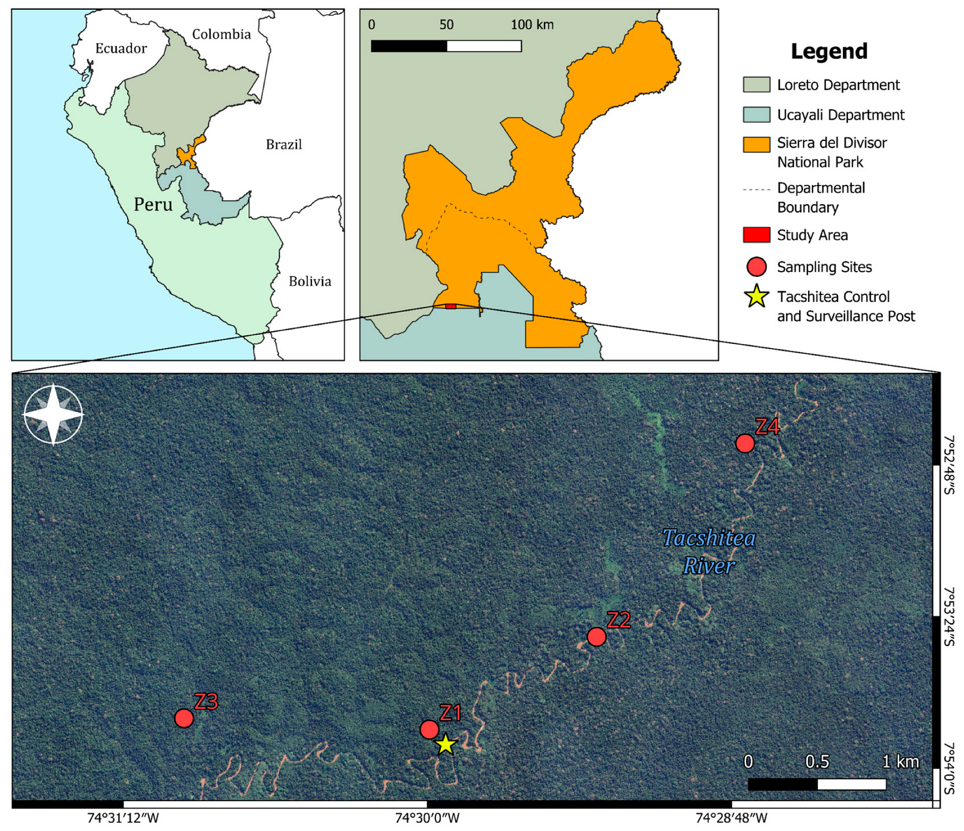
Figure 2.
Sampling zones in the Tacshitea sector: (a) semi-dense floodplain forest (Z1); (b) hillslope forest (Z2); (c) hillslope forest associated with secondary growth (Z3); (d) Mauritia flexuosa palm forest (Z4).
Figure 2.
Sampling zones in the Tacshitea sector: (a) semi-dense floodplain forest (Z1); (b) hillslope forest (Z2); (c) hillslope forest associated with secondary growth (Z3); (d) Mauritia flexuosa palm forest (Z4).
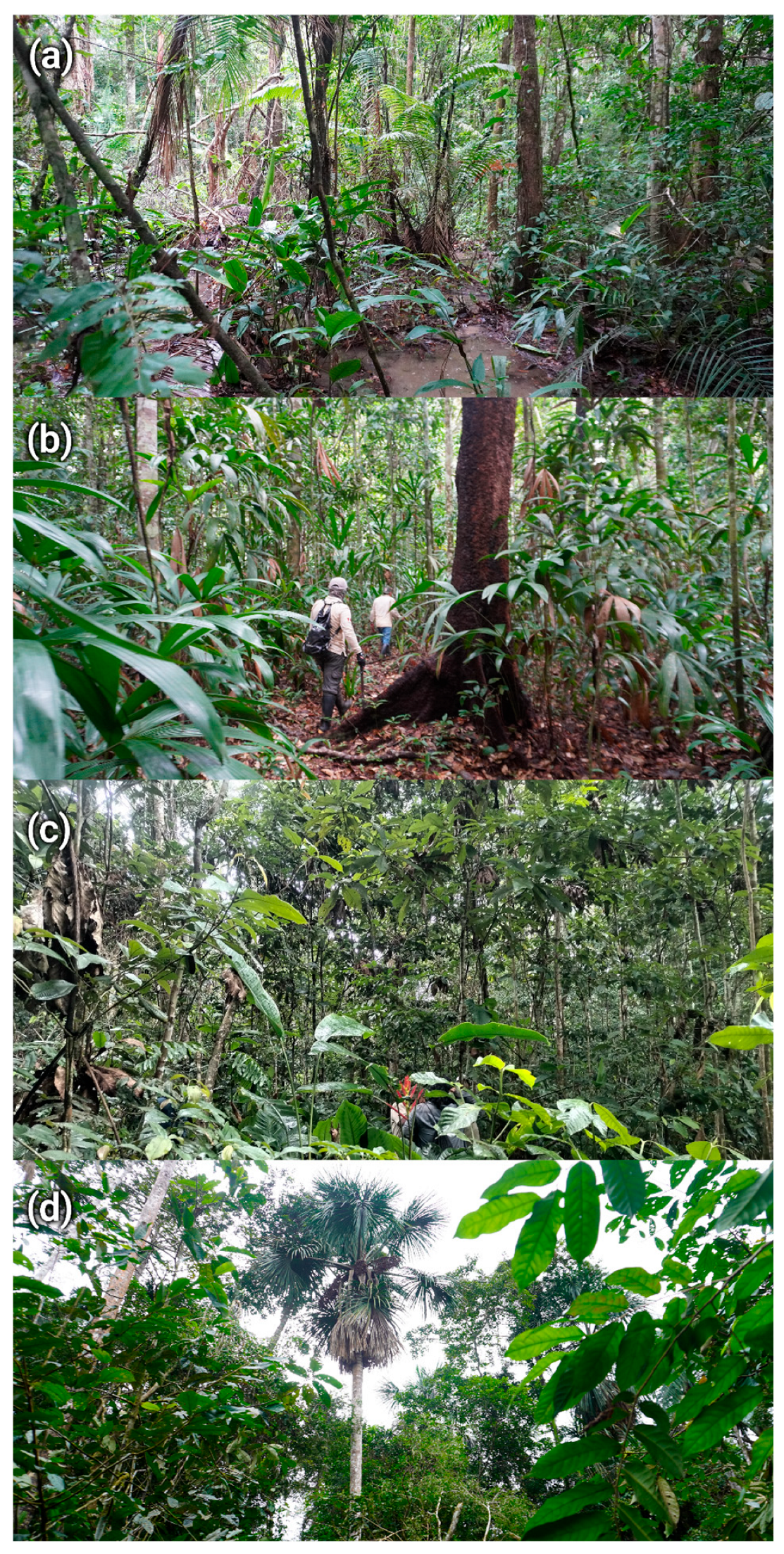
Figure 3.
Representation of vertical stratification in three levels. Own elaboration, based on Pretzsch (2009) [27].
Figure 3.
Representation of vertical stratification in three levels. Own elaboration, based on Pretzsch (2009) [27].
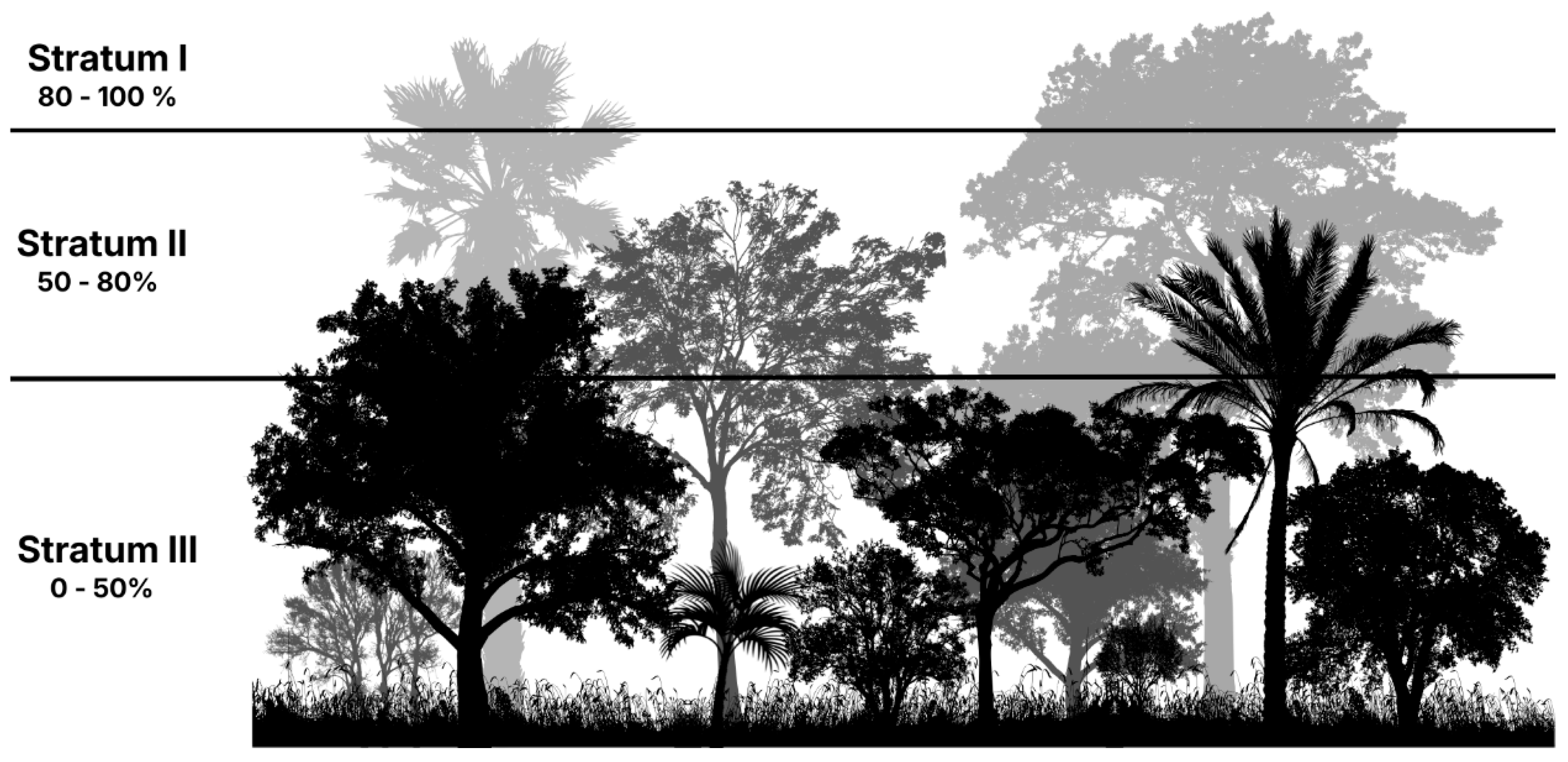
Figure 4.
Top 20 Species by Global Importance Value Index (IVI). IVI (300) = relative abundance + relative frequency + relative dominance. .
Figure 4.
Top 20 Species by Global Importance Value Index (IVI). IVI (300) = relative abundance + relative frequency + relative dominance. .
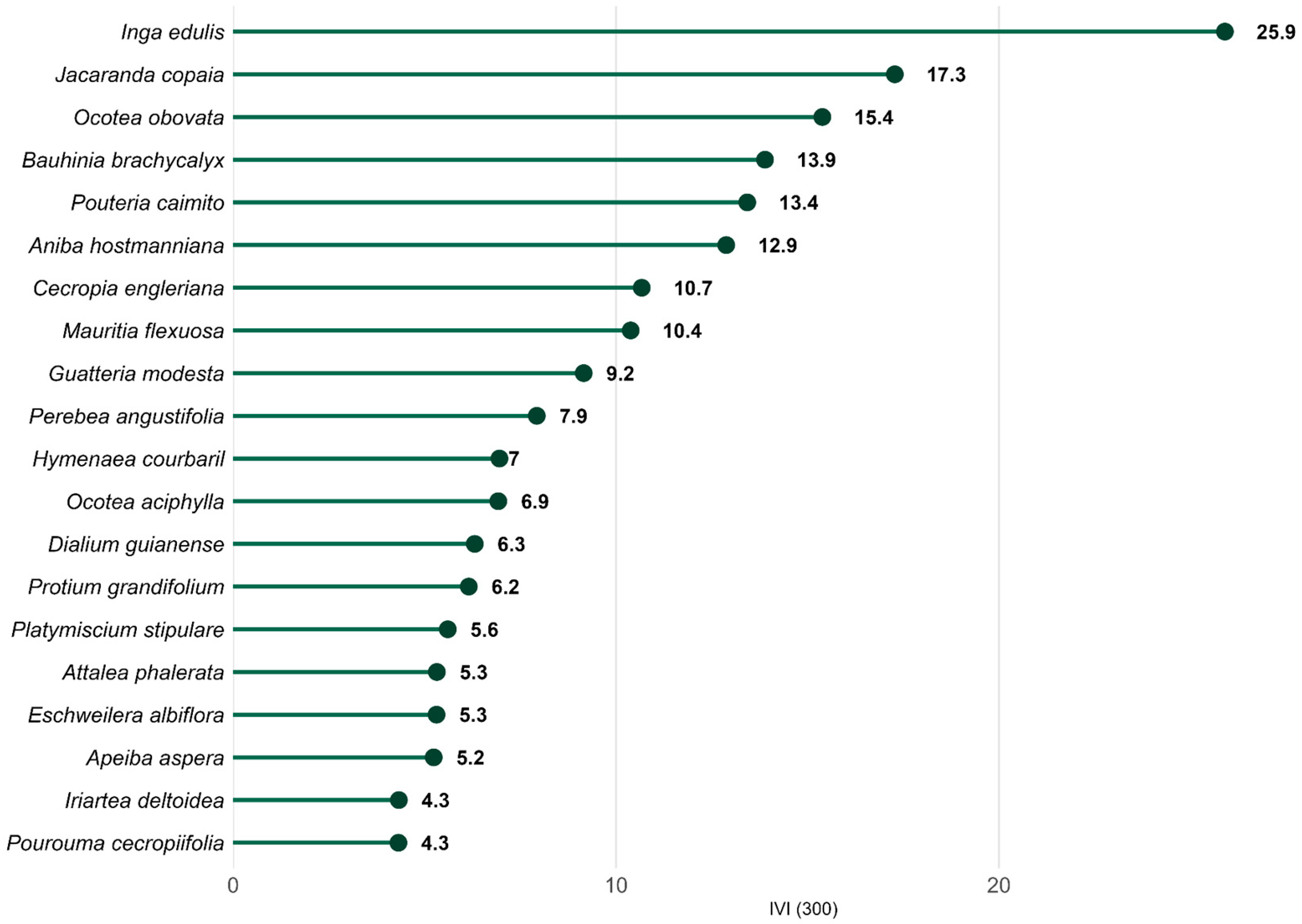
Figure 5.
Top 10 species by Importance Value Index (IVI) in each sampling zone. IVI (300) = relative abundance + relative frequency + relative dominance.
Figure 5.
Top 10 species by Importance Value Index (IVI) in each sampling zone. IVI (300) = relative abundance + relative frequency + relative dominance.
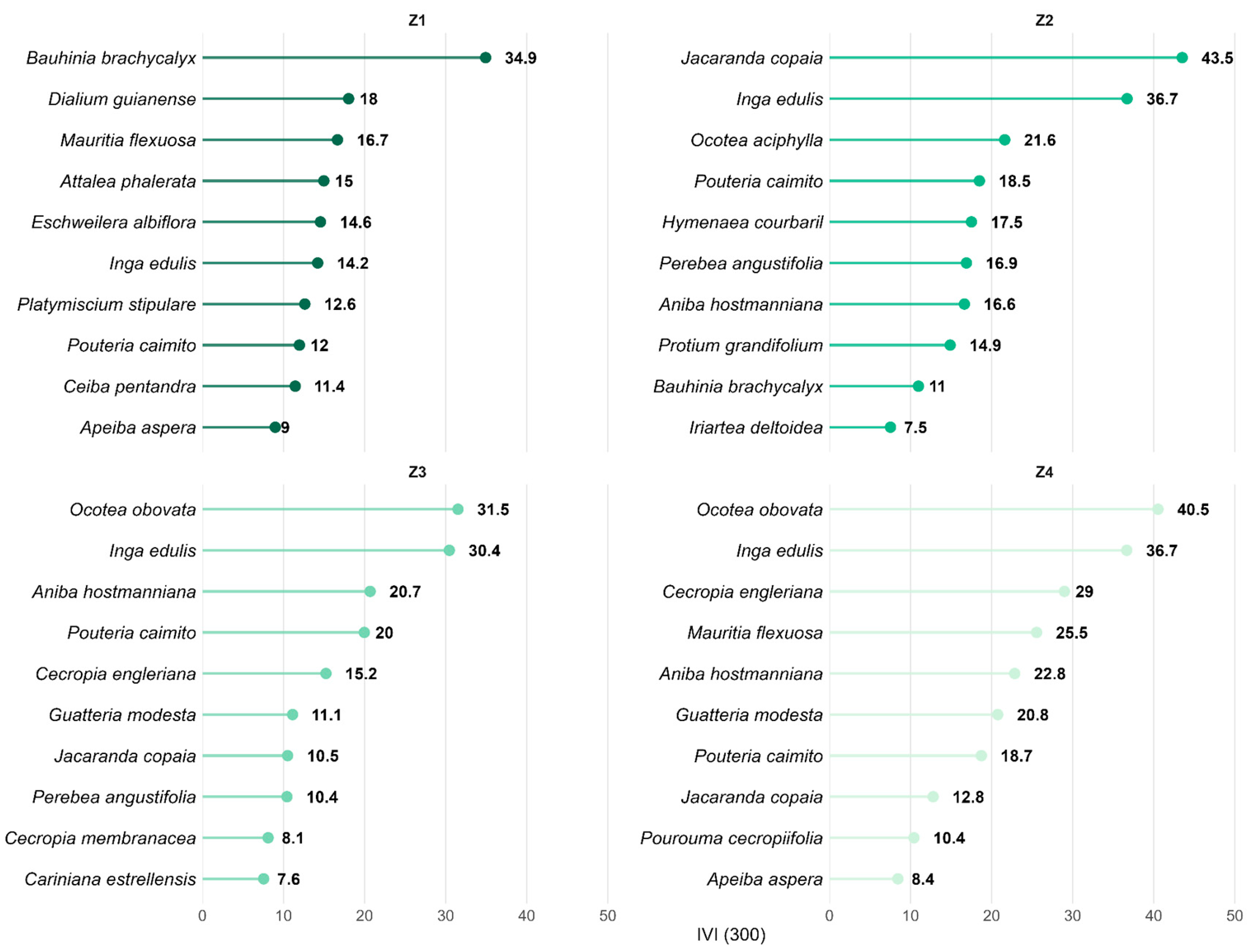
Figure 6.
Rarefaction and Interpolation/Extrapolation curves by zone based on species richness (q = 0). Solid lines represent rarefaction, dashed lines represent extrapolation, and circles indicate the observed sample size (n) for each zone, with shaded ribbons representing the 95% confidence interval.
Figure 6.
Rarefaction and Interpolation/Extrapolation curves by zone based on species richness (q = 0). Solid lines represent rarefaction, dashed lines represent extrapolation, and circles indicate the observed sample size (n) for each zone, with shaded ribbons representing the 95% confidence interval.
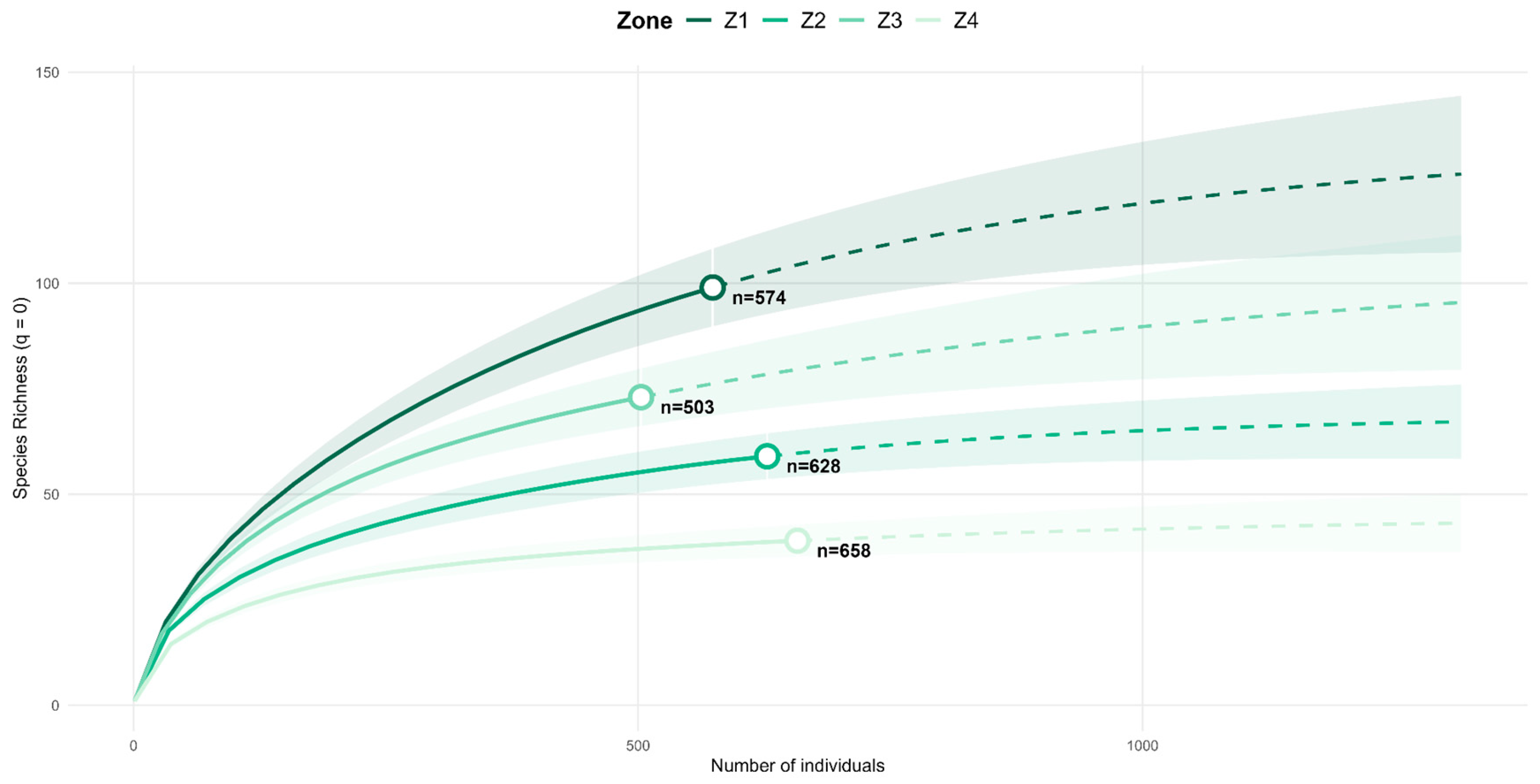
Figure 7.
Relationship between Turnover and Nestedness by pair of zones. Points represent the beta diversity components (Sørensen index) following Baselga (2010) [30]. Points toward the right indicate differences due to species turnover (Simpson index), while points upward indicate differences due to nestedness.
Figure 7.
Relationship between Turnover and Nestedness by pair of zones. Points represent the beta diversity components (Sørensen index) following Baselga (2010) [30]. Points toward the right indicate differences due to species turnover (Simpson index), while points upward indicate differences due to nestedness.
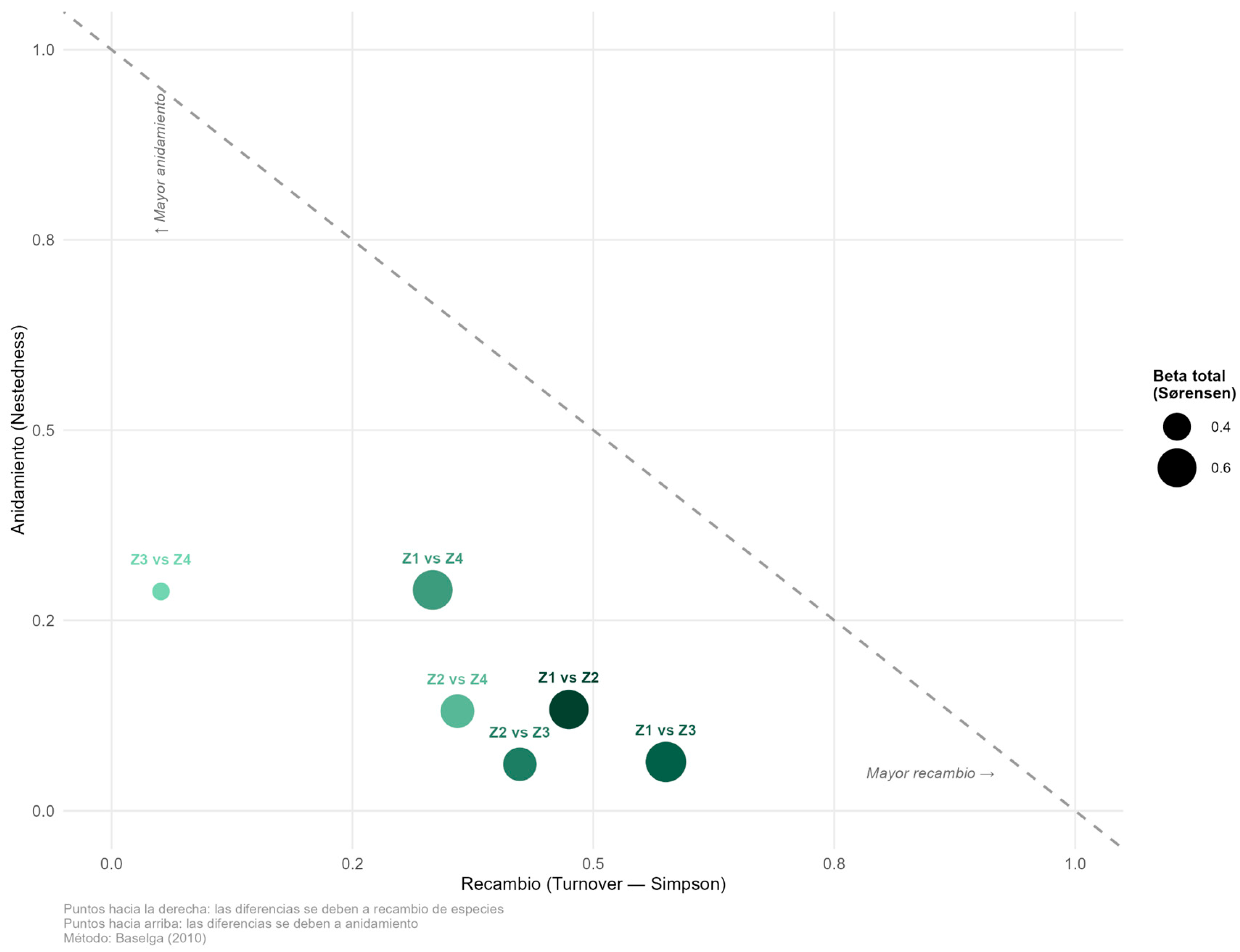
Figure 8.
SIMPER — Species contributing to differences between zones. The horizontal bar charts show the top 10 species by their average contribution to the Bray-Curtis dissimilarity for each pairwise comparison between zones (Z1 to Z4).
Figure 8.
SIMPER — Species contributing to differences between zones. The horizontal bar charts show the top 10 species by their average contribution to the Bray-Curtis dissimilarity for each pairwise comparison between zones (Z1 to Z4).
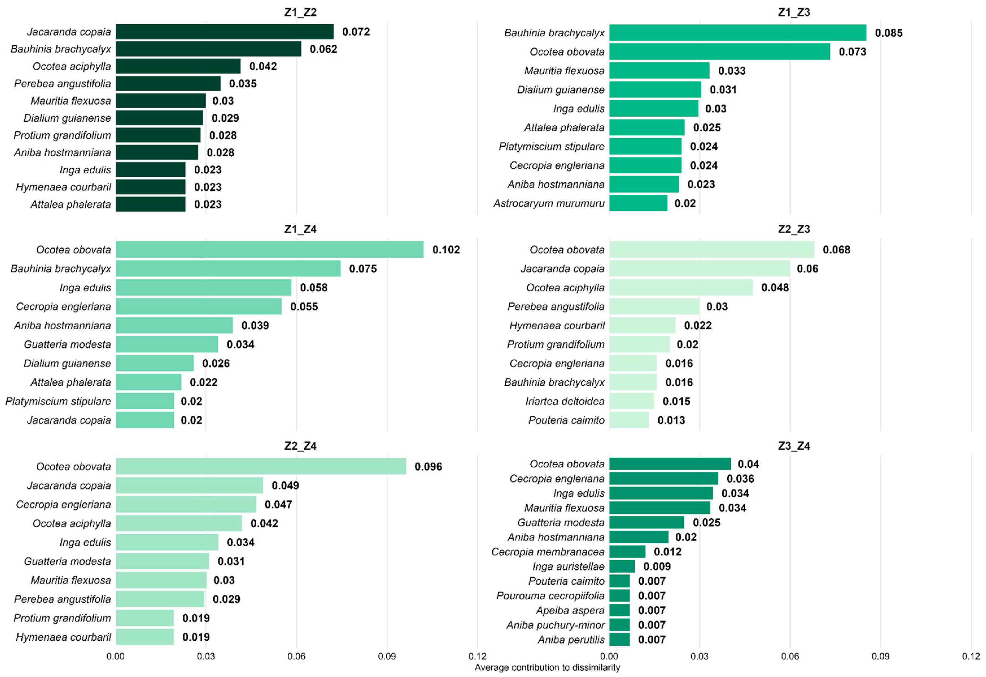
Figure 9.
Non-metric multidimensional scaling (NMDS) ordination of floristic composition among the four sampling zones based on Bray–Curtis dissimilarity. Each point represents a sampling plot, and shaded ellipses indicate the 95% confidence interval around group centroids. Stress = 0.271.
Figure 9.
Non-metric multidimensional scaling (NMDS) ordination of floristic composition among the four sampling zones based on Bray–Curtis dissimilarity. Each point represents a sampling plot, and shaded ellipses indicate the 95% confidence interval around group centroids. Stress = 0.271.
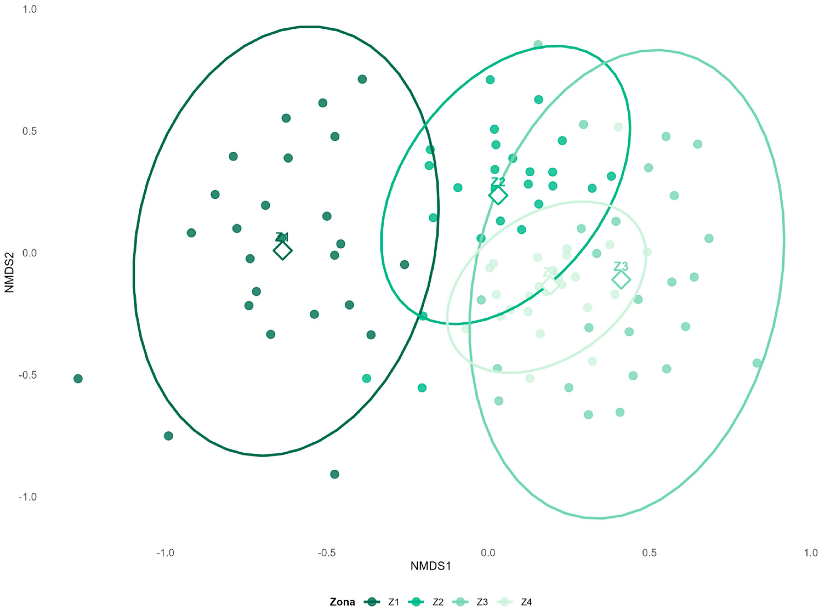
Figure 10.
Vertical structure of the sampling zones based on Pretzsch strata. The tallest tree in each zone was considered 100% of relative height, and individuals were classified into Low (0–50%), Medium (50–80%), and High (80–100%) strata. Numbers above the bars indicate abundance and relative frequency (%). ADBHted from Aguirre Calderón (2002) and Pretzsch (2009) [26,27].
Figure 10.
Vertical structure of the sampling zones based on Pretzsch strata. The tallest tree in each zone was considered 100% of relative height, and individuals were classified into Low (0–50%), Medium (50–80%), and High (80–100%) strata. Numbers above the bars indicate abundance and relative frequency (%). ADBHted from Aguirre Calderón (2002) and Pretzsch (2009) [26,27].
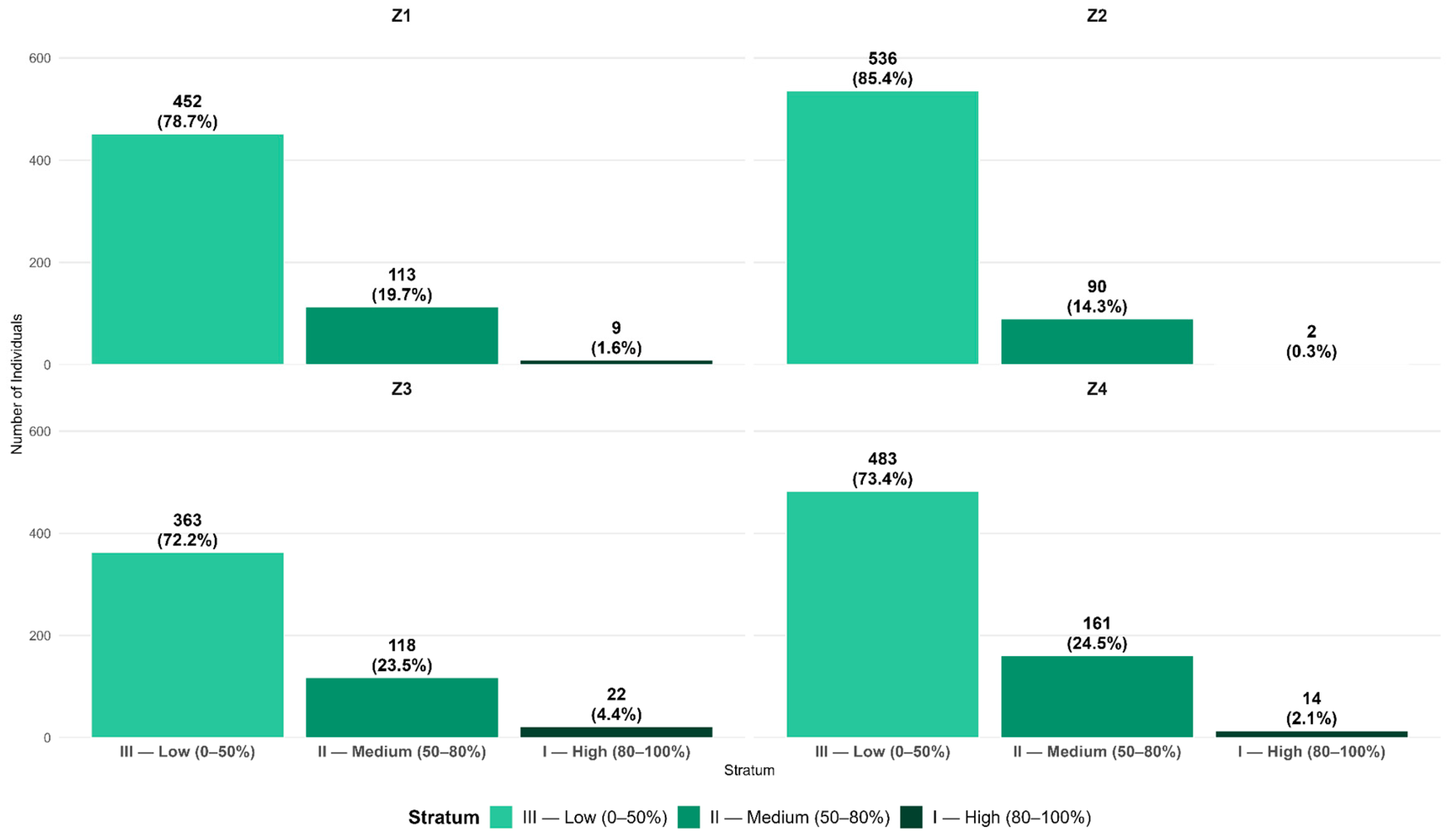
Figure 11.
Diameter class distribution by zone. Relative abundance (%) of individuals across 10-cm diameter at breast height (DBH) classes in the four sampling zones. Bars represent the percentage of individuals within each diameter class relative to the total number of individuals recorded in each zone.
Figure 11.
Diameter class distribution by zone. Relative abundance (%) of individuals across 10-cm diameter at breast height (DBH) classes in the four sampling zones. Bars represent the percentage of individuals within each diameter class relative to the total number of individuals recorded in each zone.
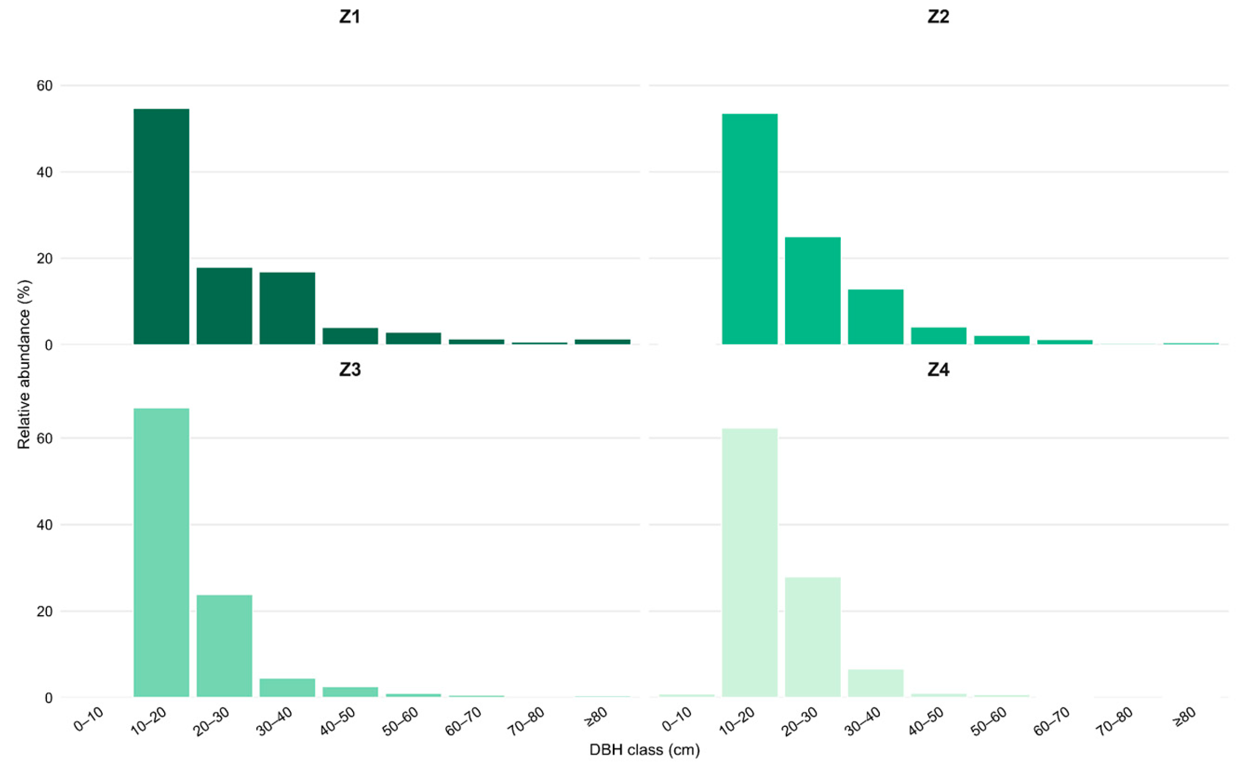
Figure 12.
Height class distribution by zone. Relative abundance (%) of individuals across five height classes (<5 m, 5–11.9 m, 12–19.9 m, 20–29.9 m, and ≥30 m) in the four sampling zones. Bars represent the percentage of individuals within each height class relative to the total number of individuals recorded in each zone.
Figure 12.
Height class distribution by zone. Relative abundance (%) of individuals across five height classes (<5 m, 5–11.9 m, 12–19.9 m, 20–29.9 m, and ≥30 m) in the four sampling zones. Bars represent the percentage of individuals within each height class relative to the total number of individuals recorded in each zone.
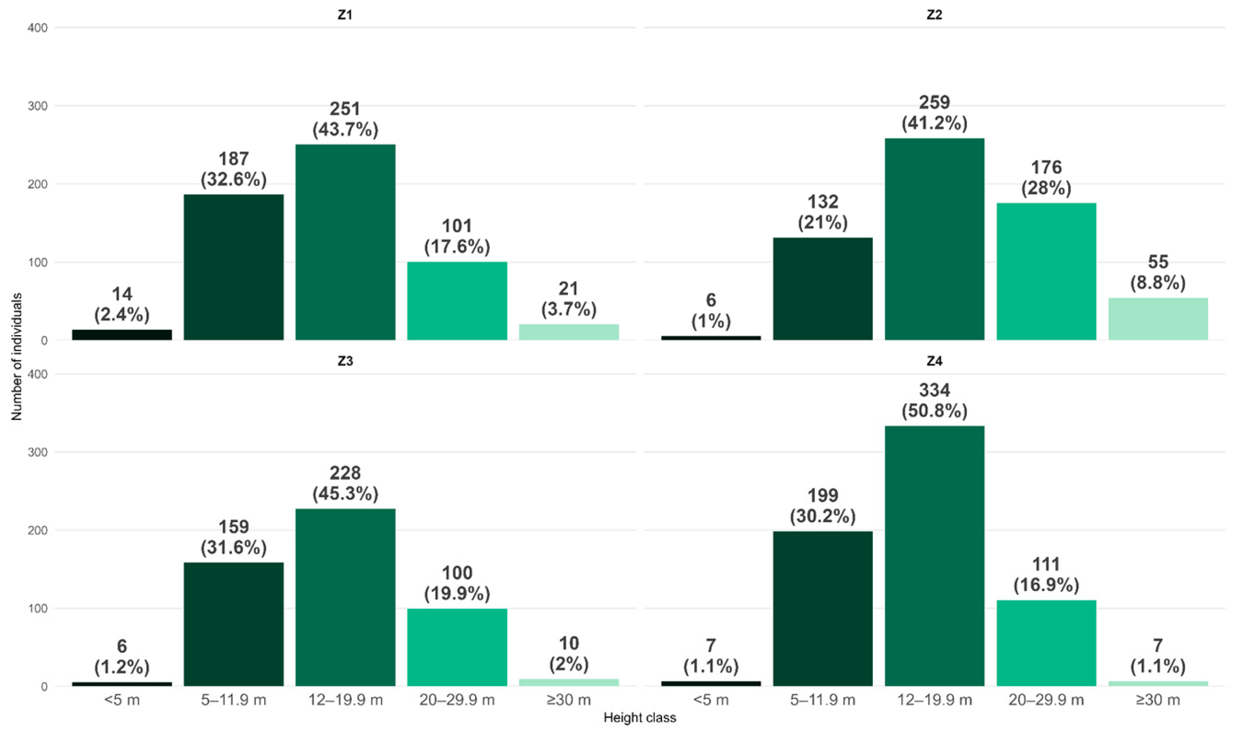
Figure 13.
Comparison of forest structural variables among zones. Boxplots showing Diameter at Breast Height (DBH), tree height, basal area, and stem volume across the four sampling zones (Z1–Z4). Boxes represent the interquartile range (Q1–Q3), the horizontal line indicates the median, and diamonds represent the mean. Different letters indicate statistically significant differences among zones according to Dunn–Bonferroni post-hoc tests (α = 0.05). Log₁₀ transformation was applied to DBH, basal area, and stem volume due to right-skewed distributions.
Figure 13.
Comparison of forest structural variables among zones. Boxplots showing Diameter at Breast Height (DBH), tree height, basal area, and stem volume across the four sampling zones (Z1–Z4). Boxes represent the interquartile range (Q1–Q3), the horizontal line indicates the median, and diamonds represent the mean. Different letters indicate statistically significant differences among zones according to Dunn–Bonferroni post-hoc tests (α = 0.05). Log₁₀ transformation was applied to DBH, basal area, and stem volume due to right-skewed distributions.
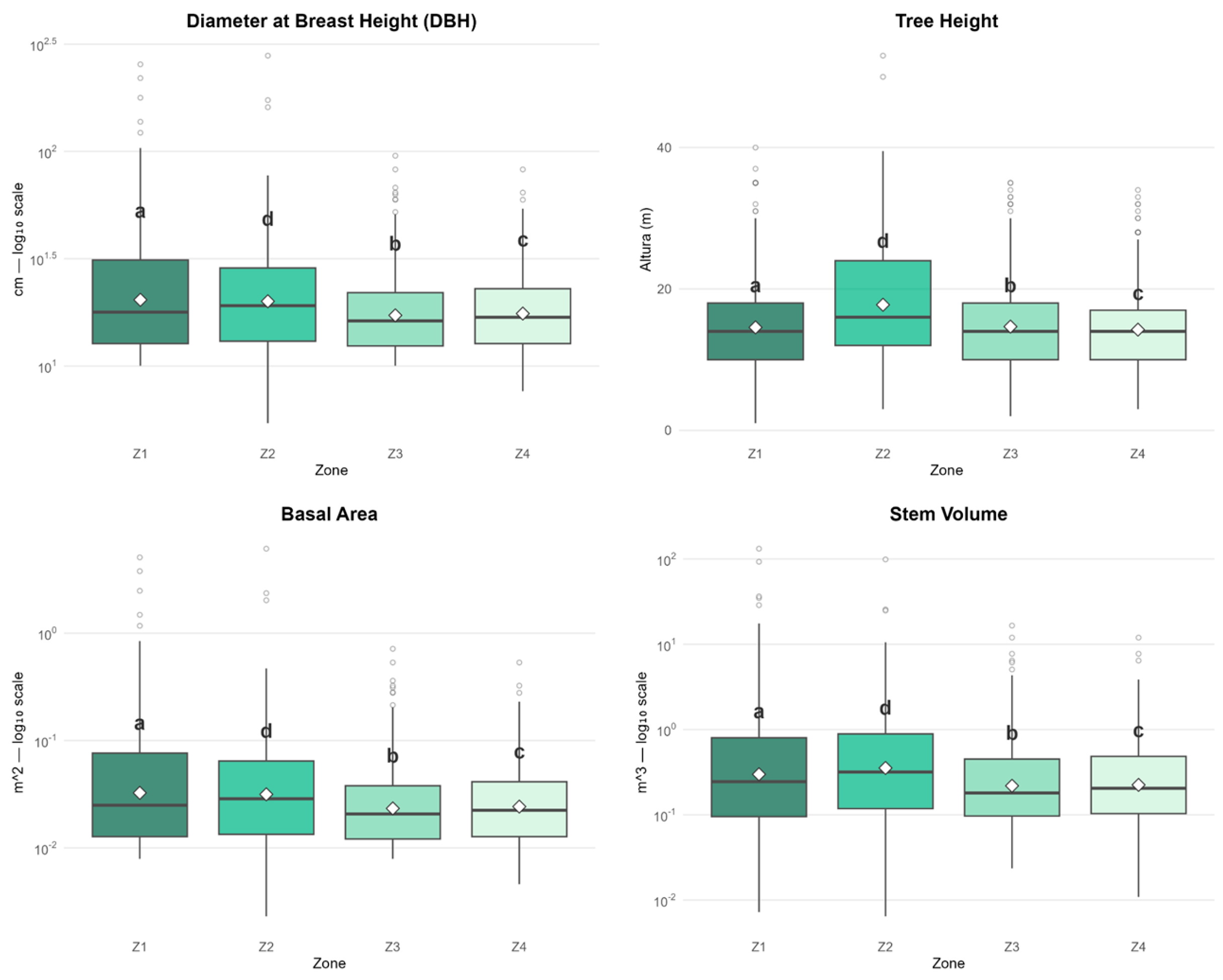
Figure 14.
Aboveground biomass and carbon stocks by vegetation unit. Total aboveground biomass (Mg ha⁻¹) and carbon stock (Mg C ha⁻¹) estimated for each sampled vegetation unit (Z1–Z4), based on all measured individuals within 1-ha plots. Bars represent total accumulated biomass and carbon per hectare in each unit.
Figure 14.
Aboveground biomass and carbon stocks by vegetation unit. Total aboveground biomass (Mg ha⁻¹) and carbon stock (Mg C ha⁻¹) estimated for each sampled vegetation unit (Z1–Z4), based on all measured individuals within 1-ha plots. Bars represent total accumulated biomass and carbon per hectare in each unit.
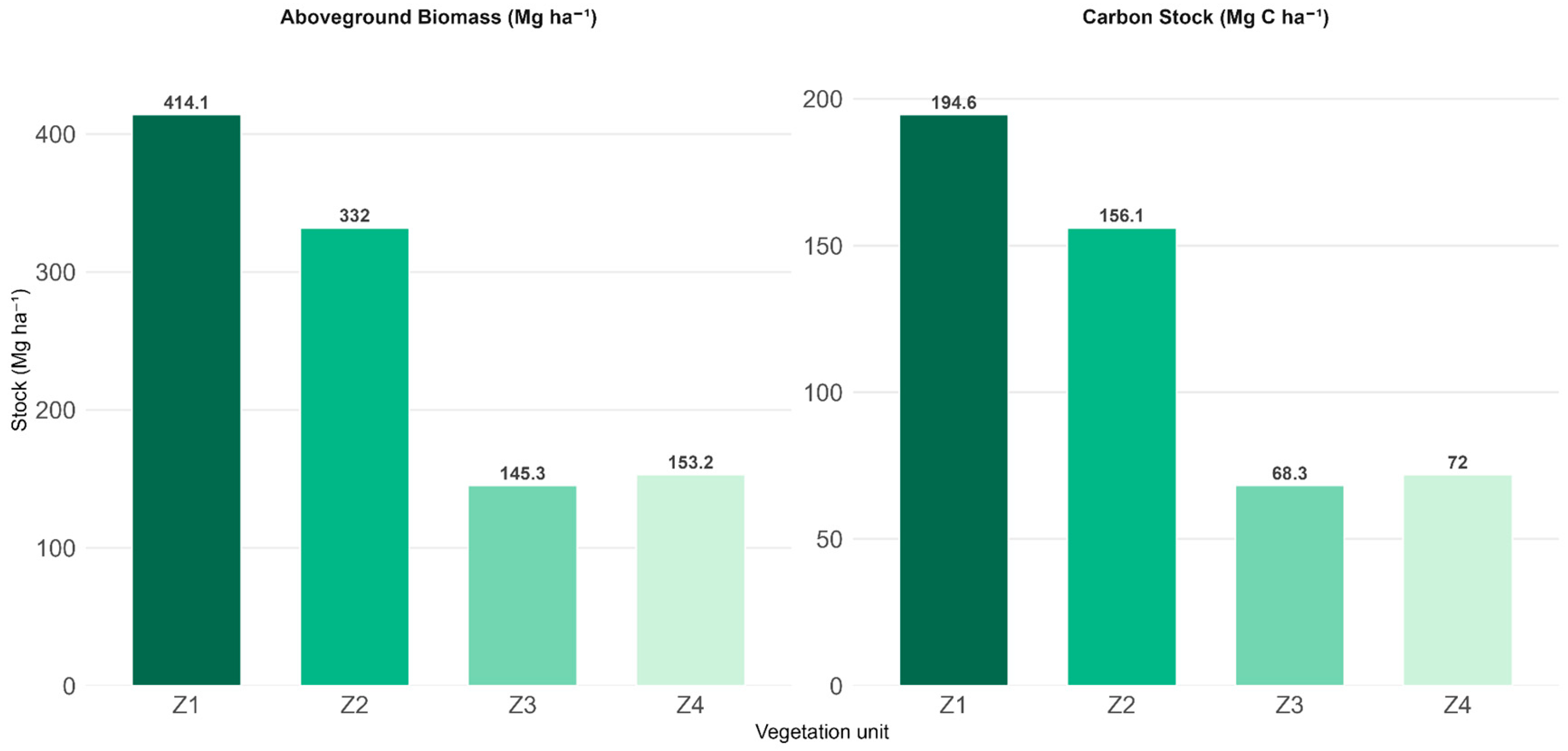
Figure 15.
Global carbon stock treemap by family (Top 15). The area of each rectangle is proportional to the total aboveground carbon stock (Mg C) contributed by each botanical family. The top 15 families are shown individually, while all remaining families are grouped into the “Others” category.
Figure 15.
Global carbon stock treemap by family (Top 15). The area of each rectangle is proportional to the total aboveground carbon stock (Mg C) contributed by each botanical family. The top 15 families are shown individually, while all remaining families are grouped into the “Others” category.
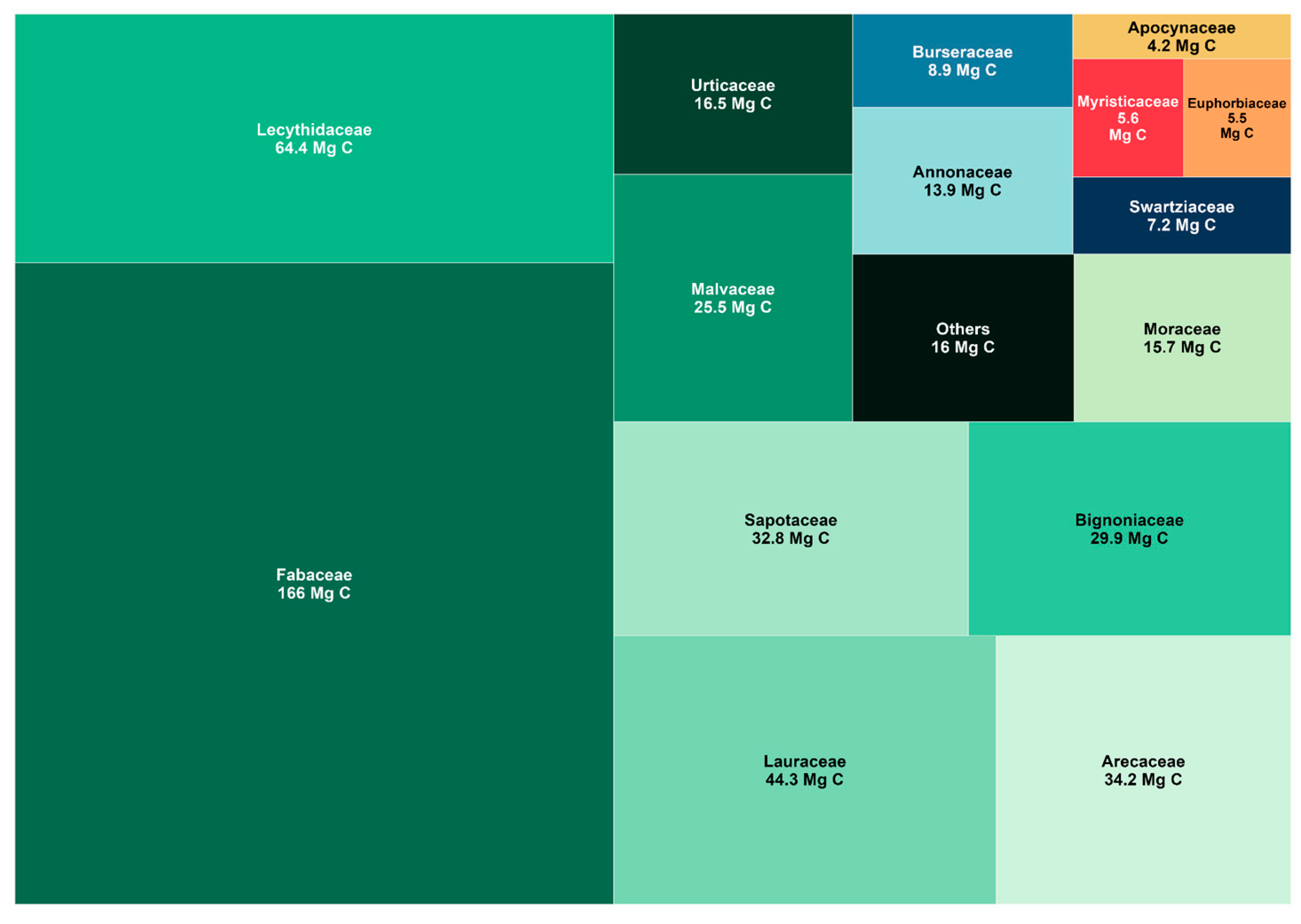
Figure 16.
Top 10 plant families contributing to aboveground carbon stock by zone. Lollipop plots showing total aboveground carbon stock (Mg C) contributed by the ten most important botanical families within each study zone (Z1–Z4).
Figure 16.
Top 10 plant families contributing to aboveground carbon stock by zone. Lollipop plots showing total aboveground carbon stock (Mg C) contributed by the ten most important botanical families within each study zone (Z1–Z4).
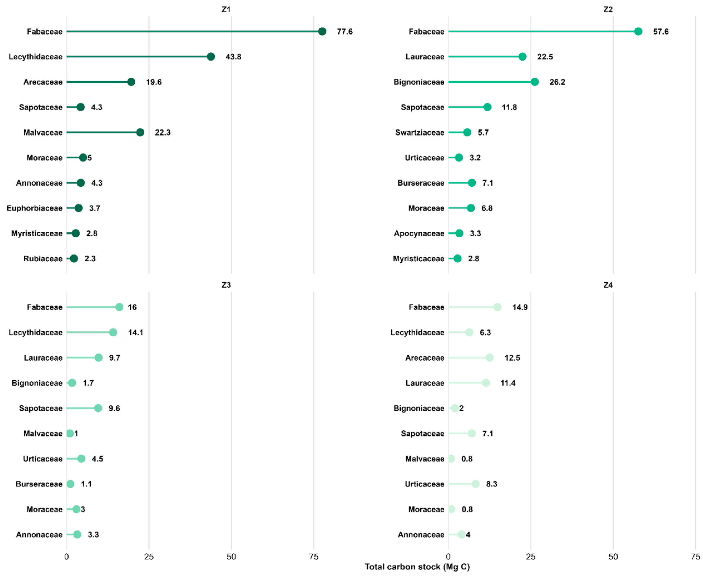
Figure 17.
Carbon distribution by Pretzsch stratum and zone. The boxplots show carbon values on a log10 scale, where boxes represent Q1–Q3, the horizontal line represents the median, and the white diamond indicates the mean for each vertical stratum (I — Upper, II — Middle, III — Lower).
Figure 17.
Carbon distribution by Pretzsch stratum and zone. The boxplots show carbon values on a log10 scale, where boxes represent Q1–Q3, the horizontal line represents the median, and the white diamond indicates the mean for each vertical stratum (I — Upper, II — Middle, III — Lower).
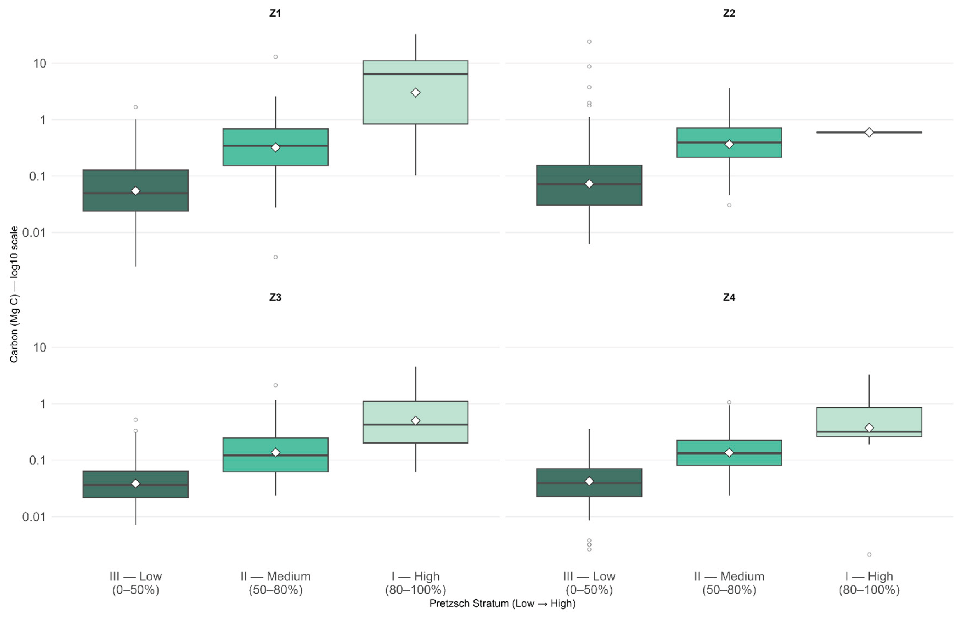

Table 1.
General characterization of the forest inventory by zone.
| Zone | N plots | Area (ha) | N orders | N families | N species | N individuals |
|---|---|---|---|---|---|---|
| Z1 | 25 | 1 | 21 | 37 | 99 | 574 |
| Z2 | 25 | 1 | 14 | 23 | 59 | 628 |
| Z3 | 25 | 1 | 16 | 27 | 73 | 503 |
| Z4 | 25 | 1 | 15 | 19 | 39 | 658 |
| Total | 100 | 4 | 24 | 41 | 158 | 2363 |
Table 2.
Alpha diversity indices by zone.
| Zone | S (Richness) | N (abund.) | H' Shannon | 1-D Simpson | J' Pielou | α Fisher | DMg Margalef |
|---|---|---|---|---|---|---|---|
| Z1 | 99 | 574 | 3,636 | 0,946 | 0,791 | 34,492 | 15,427 |
| Z2 | 59 | 628 | 3,209 | 0,938 | 0,787 | 15,955 | 9,003 |
| Z3 | 73 | 503 | 3,425 | 0,939 | 0,798 | 23,469 | 11,574 |
| Z4 | 39 | 658 | 2,759 | 0,903 | 0,753 | 9,075 | 5,856 |
Note. S = species richness; N = total abundance; H' = Shannon entropy; 1-D = Simpson diversity index; J' = Pielou evenness; α = Fisher's alpha; DMg = Margalef richness index.
Table 3.
Pairwise beta diversity indices between zones.
| Zone Pair | Bray-Curtis (sim) | Jaccard (sim) | Sørensen (sim) | Bray-Curtis (dis) | Jaccard (dis) | Sørensen (dis) |
|---|---|---|---|---|---|---|
| Z1 vs Z2 | 0.2945 | 0.2441 | 0.3924 | 0.7055 | 0.7559 | 0.6076 |
| Z1 vs Z3 | 0.2507 | 0.2199 | 0.3605 | 0.7493 | 0.7801 | 0.6395 |
| Z1 vs Z4 | 0.2776 | 0.2321 | 0.3768 | 0.7224 | 0.7679 | 0.6232 |
| Z2 vs Z3 | 0.4527 | 0.3469 | 0.5152 | 0.5473 | 0.6531 | 0.4848 |
| Z2 vs Z4 | 0.3966 | 0.3425 | 0.5102 | 0.6034 | 0.6575 | 0.4898 |
| Z3 vs Z4 | 0.6546 | 0.4933 | 0.6607 | 0.3454 | 0.5067 | 0.3393 |
Note. sim = similarity; dis = dissimilarity (0 = no shared species; 1 = identical). Bray-Curtis: abundance-based. Jaccard and Sørensen: presence/absence.
Table 4.
Permutational multivariate analysis of variance (PERMANOVA) of floristic composition between zones.
Table 4.
Permutational multivariate analysis of variance (PERMANOVA) of floristic composition between zones.
| Source of variation | gl | SC | R² | F | p-valor |
|---|---|---|---|---|---|
| Model | 3 | 8.1138 | 0.2652 | 11.5483 | 0.001 |
| Residual | 96 | 22.4831 | 0.7348 | ||
| Total | 99 | 30.5969 | 1 |
Note. gl = degrees of freedom; SC = sum of squares; F = F-statistic; R² = proportion of variance explained; 999 permutations. Distance: Bray-Curtis. Method: Anderson (2001) [36].
Table 5.
Results of Dunn's post-hoc test for structural variables by Pretzsch stratum (Bonferroni, p < 0.05).
Table 5.
Results of Dunn's post-hoc test for structural variables by Pretzsch stratum (Bonferroni, p < 0.05).
| Variable | Stratum | Z1–Z2 | Z1–Z3 | Z2–Z3 | Z1–Z4 | Z2–Z4 | Z3–Z4 |
|---|---|---|---|---|---|---|---|
| Height | I (upper) | ns | *** | * | *** | * | ns |
| II (middle) | ns | *** | ns | ns | ns | ** | |
| III (lower) | ns | *** | ns | ns | ns | ** | |
| Richness | I (upper) | *** | *** | *** | *** | *** | ns |
| II (middle) | *** | *** | *** | ns | *** | *** | |
| III (lower) | * | *** | *** | *** | *** | *** | |
| Abundance | I (upper) | *** | *** | *** | *** | *** | ns |
| II (middle) | *** | * | ** | *** | *** | *** | |
| III (lower) | *** | ns | *** | *** | ns | *** |
Note: Levels of statistical significance: ns = p > 0.05; * = p < 0.05; ** = p < 0.01; *** = p < 0.001. p-values adjusted using Dunn’s method.
Table 6.
Summary of structural variables.
| Parameter | Z1 | Z2 | Z3 | Z4 |
| DAP (cm) | 24.45 ± 20.82 | 23.2 ± 17.69 | 19 ± 10.21 | 18.99 ± 8.32 |
| Height (m) | 14.56 ± 6.49 | 17.76 ± 7.74 | 14.67 ± 6.17 | 14.24 ± 5.41 |
| AB ind⁻¹ (m²) | 0.0809 ± 0.3015 | 0.0668 ± 0.2779 | 0.0365 ± 0.0571 | 0.0337 ± 0.0383 |
| AB ha⁻¹ (m²) | 46.45 | 41.96 | 18.37 | 22.2 |
| Vol ind⁻¹ (m³) | 1.289 ± 7.225 | 1.015 ± 4.318 | 0.486 ± 1.183 | 0.402 ± 0.74 |
| Vol ha⁻¹ (m³) | 739.66 | 637.36 | 244.43 | 264.54 |
Note. Individual-level values are presented as mean ± SD. Hectare-level values correspond to totals recorded within each 1-ha sampling zone. AB = basal area; Vol = volume.
Table 7.
Summary of individual biomass and carbon stock by zone.
| Parameter | Z1 | Z2 | Z3 | Z4 |
| Biomass ind⁻¹ (Mg) | 0.7214 ± 3.8242 | 0.5287 ± 2.2704 | 0.2888 ± 0.7516 | 0.2328 ± 0.4852 |
| Carbon ind⁻¹ (Mg C) | 0.3391 ± 1.7974 | 0.2485 ± 1.0671 | 0.1357 ± 0.3533 | 0.1094 ± 0.228 |
Note. Individual-level values are presented as mean ± SD. Hectare-level values correspond to totals recorded within each 1-ha sampling zone.
Table 8.
Results of Dunn's post-hoc test for carbon stock by Pretzsch stratum (Bonferroni, p < 0.05).
Table 8.
Results of Dunn's post-hoc test for carbon stock by Pretzsch stratum (Bonferroni, p < 0.05).
| Variable | Stratum | Z1–Z2 | Z1–Z3 | Z2–Z3 | Z1–Z4 | Z2–Z4 | Z3–Z4 |
|---|---|---|---|---|---|---|---|
| Carbon | I (High 80–100%) | ns | ns | ns | ns | ns | ns |
| II (Medium 40–80%) | * | *** | *** | *** | *** | ns | |
| III (Low 0–40%) | * | *** | *** | *** | *** | ns |
Note: Statistical significance levels: ns = p > 0.05; * = p < 0.05; = p < 0.01; *** = p < 0.001. P-values adjusted using Dunn's method.
Table 9.
Spearman correlation matrix between diversity metrics and carbon stock.
| Shannon | Simpson | Richness | Carbon |
|---|---|---|---|
| 1 | 1 | 1 | 0.13 |
| 1 | 1 | 1 | 0.13 |
| 1 | 1 | 1 | 0.13 |
| 0.13 | 0.13 | 0.13 | 1 |
Note. Spearman correlation coefficients among diversity metrics and carbon (Mg C per plot).
Table 10.
Linear regression models between diversity metrics and carbon stock.
| Model | Estimate | SE | p_value | R2 |
|---|---|---|---|---|
| Carbon ~ Shannon | 3.954869867 | 1.836312275 | 0.033716283 | 0.045191973 |
| Carbon ~ Simpson | 81.34326875 | 35.28662236 | 0.02326339 | 0.0514356 |
| Carbon ~ Richness | 0.065608689 | 0.027161346 | 0.017565969 | 0.056192397 |
Note. Simple linear models relating carbon stock (Mg C) and diversity metrics.
Table 11.
Linear mixed-effects model explaining carbon stock variation.
| Term | Estimate | SE | t_value | p_value |
|---|---|---|---|---|
| (Intercept) | -7.972775107 | 12.49851961 | 1.999999962 | 0.588830668 |
| Shannon | 3.954869867 | 3.818148737 | 1.999999963 | 0.409111914 |
Note. Mixed-effects model with Shannon diversity as fixed effect and Zone as random intercept.
Table 12.
Conservation status, zonal distribution, and aboveground carbon stock of key species.
| Specie | UICN | DS 043-2006-AG | CITES | Presence zones | Records (N) | Global IVI (300) | Total carbon (Mg) |
|---|---|---|---|---|---|---|---|
| Aniba perutilis | VU | VU | NR | Z2, Z3 | 10 | 12.878 | 0.723 |
| Ceiba pentandra | LC | NT | NR | Z1 | 1 | 4.111 | 19.146 |
| Cinchona officinalis | VU | NC | NR | Z1 | 2 | 0.577 | 2.029 |
| Dipteryx micrantha | NT | VU | II | Z1 | 2 | 0.488 | 1.156 |
| Euterpe cf. edulis | VU | NC | NR | Z1, Z2, Z3, Z4 | 22 | 2.731 | 0.983 |
| Platymiscium stipulare | VU | NT | NR | Z1, Z2, Z3, Z4 | 34 | 5.605 | 9.365 |
| Virola surinamensis | EN | EN | NR | Z2 | 2 | 0.354 | 0.066 |
Notes: VU = Vulnerable; EN = Endangered; NT = Near Threatened; LC = Least Concern; NC = Not Categorized; NR = Not Regulated. N = Number of recorded individuals. Carbon expressed in Mg. The areas correspond to the sampling units (Z1–Z4) where the species was confirmed to be present.
Disclaimer/Publisher’s Note: The statements, opinions and data contained in all publications are solely those of the individual author(s) and contributor(s) and not of MDPI and/or the editor(s). MDPI and/or the editor(s) disclaim responsibility for any injury to people or property resulting from any ideas, methods, instructions or products referred to in the content. |
© 2026 by the authors. Licensee MDPI, Basel, Switzerland. This article is an open access article distributed under the terms and conditions of the Creative Commons Attribution (CC BY) license (http://creativecommons.org/licenses/by/4.0/).
Copyright: This open access article is published under a Creative Commons CC BY 4.0 license, which permit the free download, distribution, and reuse, provided that the author and preprint are cited in any reuse.