

Submitted:
20 August 2026
Posted:
20 August 2026
You are already at the latest version
Abstract
Corrective congestion management in a transmission network with embedded HVDC requires coordinating continuous set-points and discrete topological actions under the full nonlinear AC power flow constraints, a mixed-integer nonlinear problem for which no polynomial-time solution is known. This paper formulates the task as a Markov decision process and solves it with a hybrid Soft Actor-Critic agent that handles both action types under one maximum-entropy objective: a squashed-Gaussian head for redispatch and the VSC-HVDC set-point, and two categorical heads trained through the Gumbel-Softmax Straight-Through estimator for generator and line disconnection. Each action subspace carries its own entropy temperature rather than a shared coefficient, and the behaviour of the three is measured. The state is 906-dimensional and covers branch loadings and reactive flows, bus voltages and angles, and the HVDC set-point. On the IEEE 118-bus system extended with a VSC-HVDClink,theagentclears98.6%ofa500-scenariointact-gridbatch and 97.4% of a 500-scenario batch that includes up to three simultaneous branch outages, in a mean of 1.5 and 1.7 corrective steps respectively, with an independent AC verification power flow confirming the resulting states. Inference requires a single forward pass, which makes the policy usable inside an operational decision cycle.
Keywords:
hybrid discrete-continuous action space
; Gumbel-Softmax Straight-Through
; soft actor-critic
; AC power flow
; VSC-HVDC
; corrective congestion management
; entropy temperature
; IEEE 118-bus
1. Introduction
1.1. Computational Hardness of the AC-OPF
The AC optimal power flow (AC-OPF) is a continuous non-convex nonlinear program whose feasible set is generally non-connected because of voltage magnitude and angle constraints [1,2]. Classical interior-point solvers [3] reach local optima in seconds for medium-scale systems, but global optimality guarantees require semidefinite relaxations [4] or branch-and-bound enumeration, both computationally prohibitive in real time. The security-constrained AC-OPF adds N-1 contingency constraints that multiply the problem size by the number of contingency cases [5,6,7,8], which places the problem beyond the redispatch cycle even for medium-sized systems. The ARPA-E Grid Optimization competitions [9,10,11] have benchmarked the state of the art and show that a substantial gap remains between solver runtime and real-time requirements.
1.2. The Hybrid Action Space
Corrective congestion management in a real transmission network involves both continuous and discrete decisions. On the continuous side, generators adjust active output within ramp limits [12] and HVDC links modulate the scheduled power transfer [13]. On the discrete side, network topology is modified by switching lines, transformers, or busbar sections [14,15]. The two interact strongly through the power flow equations: opening a line changes the effective distribution factors [16], which in turn changes the optimal continuous redispatch.
Handling hybrid action spaces in deep reinforcement learning is not straightforward. DQN [17] and its extensions handle only discrete actions; on-policy methods such as PPO [18] can in principle handle both but sacrifice sample efficiency; and standard SAC [19,20] and TD3 [21] handle only continuous actions. Parametrised DQN [22] extends DQN to hybrid spaces by maintaining a separate continuous parameter network, at the cost of a Q-network that must enumerate every discrete choice. The Gumbel-Softmax distribution [23,24] offers a different route: a differentiable continuous relaxation of categorical variables that permits gradient-based optimisation of the discrete decision while preserving the actor-critic structure of SAC. That is the route taken here.
1.3. VSC-HVDC in the Training Environment
VSC-HVDC links are increasingly deployed in transmission grids to improve transfer capacity, controllability and renewable integration [1,13]. Their quasi-static model introduces decoupled active power injections at the rectifier and inverter terminals, with converter losses that grow with the transmitted power [13]. Unlike reactive compensation devices, a VSC-HVDC link controls active power flow directly across long distances, which makes it a first-line instrument for congestion relief rather than an auxiliary one. The companion paper [25] describes the scenario generator that produced the training corpus, including the genotype from which each episode is initialised.
1.4. Contributions
The contributions of this paper are:
- a hybrid SAC architecture that unifies continuous redispatch, continuous HVDC control and discrete topology switching under a single maximum-entropy objective;
- the application of the Gumbel-Softmax Straight-Through estimator to topology switching in a full AC 118-bus environment, which makes the discrete heads trainable by backpropagation;
- one entropy temperature per action subspace (, , ), for subspaces whose entropy scales are not commensurable, together with a measurement of how each of the three behaves over training;
- a 906-dimensional state encoding that exposes full AC observability, including reactive branch flows, bus voltages and angles, and the HVDC set-point; and
- an evaluation on two independent 500-scenario batches and on a 1806-scenario out-of-training corpus, with every reported action verified by an independent AC power flow.
The rest of the paper is organised as follows. Section 2 describes the AC environment and its solver; Section 3 presents the hybrid SAC architecture; Section 4 gives the MDP formulation and the training protocol; Section 5 reports the experimental results; and Section 6 discusses them and concludes.
2. AC Environment and Power Flow Solver
2.1. Newton–Raphson AC Power Flow
The AC power flow equations enforce complex power balance at each bus:
where and are the voltage magnitude and angle at bus i and is the corresponding entry of the bus admittance matrix [1,2,26,27]. The Newton–Raphson iteration solves the mismatch system with by iterating
with the block-structured Jacobian
CasADi [28] with the KLU sparse direct solver [29] evaluates (2) by exploiting the sparsity of the admittance matrix [2,30] and by pre-computing the symbolic Jacobian once at initialisation. Convergence is declared at with a limit of 50 iterations.
The environment uses two solver modes by design. At reset() the power flow is solved with the outer control loop enabled, so that on-load tap changers and switched shunts converge to a consistent position, which is then frozen. At every subsequent step() the plain Newton–Raphson solver is used with those devices held fixed. The asymmetry is deliberate: the outer loop is several times more expensive than a plain solve, and running it once per episode preserves the physical coherence of the initial state without paying its cost at every interaction.
2.2. VSC-HVDC Quasi-Static Model
The VSC-HVDC link (bus 89 → bus 12) is modelled as two coupled active power injections [13]:
where is the quadratic converter loss characteristic. Each terminal is rated at 300 MVA, so the set-point is bounded by on a 100 MVA base. The agent does not command directly: it commands an increment with , and the resulting set-point is clipped to the admissible interval. One unit of action therefore spans half the converter rating, which lets the agent traverse the full range in two steps while retaining fine control.
2.3. Episode Initialisation and the Load-Scaling Defect
Each episode is initialised from a genotype [25]. The reset() method applies the generator dispatch , the load scaling , the topology and the HVDC transfer , and then solves the power flow with the outer control loop. An episode is accepted when at least one branch satisfies after convergence.
An earlier version of reset() omitted the factor when initialising the demand vectors, a defect documented in [25]. Without every load defaulted to its base-case value, so the training distribution was systematically less loaded than the distribution used for evaluation. The agent trained on that corpus plateaued at 71.0% success rate while its training curves looked healthy; applying before the power flow solve raised the same configuration to 98.6%, an improvement of 27.6 percentage points that exceeds every architectural change reported in this paper. All results below were obtained after the correction.
3. Hybrid SAC Architecture
3.1. Decomposition of the Action Space
The action space is decomposed into three subspaces:
- Continuous (): 53 per-generator active redispatch increments for the non-slack generators, plus the HVDC set-point increment, parametrised by the standard squashed-Gaussian actor of SAC [20];
- Discrete generator head (): index of the generator to disconnect, with the null action at index 0 and four pre-curated candidates at buses 46, 54, 87 and 111;
- Discrete line head (): index of the line to open, with the null action at index 0 and thirteen candidates formed by five parallel pairs and three single circuits.
The generator at bus 12 and the lines 89–90 and 89–92 are excluded from the candidate sets because they are directly adjacent to the terminals of the VSC-HVDC link (bus 89 and bus 12); switching them would remove the very degree of freedom the agent is meant to exploit. Figure 1 shows the resulting architecture.
3.2. Gumbel-Softmax Straight-Through Estimator
Discrete topology actions are inherently non-differentiable: the operation that selects a branch to switch blocks gradient flow through the actor network, which prevents standard backpropagation from training the discrete heads. For a categorical variable with probabilities , the Gumbel-Softmax distribution [23,24] draws
where is the temperature. As the relaxation concentrates on the class and approaches the one-hot representation. The Straight-Through variant [23] uses the hard one-hot vector in the forward pass and the soft vector in the backward pass:
with the stop-gradient operator. The discrete structure is therefore exact at execution time while the gradient still flows during training. The temperature is annealed geometrically towards a floor,
with , and a per-update rate , so the floor is reached after roughly gradient updates.
3.3. Per-Subspace Entropy Temperatures
Standard SAC uses a single temperature for the entropy of the whole policy. In the hybrid setting the three subspaces have entropy scales that are not commensurable: the entropy of the continuous Gaussian head depends on 54 log standard deviations, whereas the entropy of a categorical head is bounded by and respectively. A single temperature therefore produces conflicting gradient signals and leaves at least one head at an inappropriate exploration level.
Three independent temperatures are introduced, each minimising its own loss:
with target entropies , and : the conventional SAC target for a 54-dimensional continuous action, and one target per categorical head scaled by the size of its catalogue. The coefficients are stored in logarithmic form and clamped independently to and . The total entropy term entering both the critic target and the actor loss is
What the three coefficients actually do during training is worth reporting, because only one of them adapts. Across both full-length runs, and leave their initial value within the first few thousand updates and then sit at the lower clamp for the remainder of training: their 25th percentile, median and 75th percentile over the run all coincide with that bound. Only tracks its target, oscillating between 0.136 and 0.42 with a run mean of 0.197–0.207 depending on the seed. In the configuration reported here, therefore, the mechanism behaves as one adaptive temperature for the continuous head plus two categorical heads held at minimum entropy pressure. Section 5 returns to this when examining which switching actions the agent actually uses.
3.4. State Space: 906-Dimensional AC Observability
The observation is a flat 906-dimensional vector composed of the ten blocks listed in Table 1. Two design choices deserve comment. First, the reactive branch flows are included alongside the apparent loading, which lets the agent distinguish a branch that is thermally loaded by active transit from one loaded by reactive circulation—a distinction that does not exist in a DC formulation and that determines whether redispatch or topology is the effective remedy. Second, the availability flags of the four candidate generators are included so that the discrete head can observe which of its own options remain, rather than having to infer it from the dispatch vector.
3.5. Networks and Hyperparameters
The actor uses a shared MLP trunk that splits into three heads: a continuous head producing , a generator head with logits , and a line head with logits . The critic consists of twin Q-networks with hidden layers , which take the concatenation of dimension 73 alongside the observation; the twin structure mitigates overestimation bias [21]. Table 2 lists the full configuration.
4. MDP Formulation and Training Protocol
4.1. Transition and Reward
The composite action at step t is . The transition applies the redispatch and the HVDC increment, opens the selected generator or line if the corresponding index is non-null, and re-solves the AC power flow on the modified network. The reward combines a quadratic overload penalty, a redispatch cost, a switching cost and a terminal success bonus:
with , MW−1, and . The coefficients are named and rather than and to avoid collision with the entropy temperatures of Section 3.3 and with the discount factor. The redispatch increments are expressed in MW, so converts megawatts into reward units; the expression is a per-step quantity and the episode return is its sum over the steps taken. The quadratic form of the first term makes a severe overload attract far more corrective pressure than a marginal one, which directs the policy towards the critical branch when several are violated at once. The HVDC increment carries no explicit cost, a deliberate design choice: moving power through an existing converter does not incur the redispatch payments that a generator adjustment does.
An episode terminates successfully when every branch satisfies , and is truncated at steps. If the Newton–Raphson solver fails to converge after an action, the environment reverts the network to its previous state, returns a penalty of and continues the episode rather than ending it. This is a deliberate departure from the more common practice of terminating on divergence: a non-convergent action is an unusable recommendation, not a system collapse, and letting the episode continue allows the agent to propose an alternative within the same decision cycle.
4.2. Scenario Sampling and Training Protocol
Episodes are drawn from the 253,378-scenario AC corpus of [25]. Sampling is stratified over the groups formed by the overload threshold and the outage catalogue of each shard, so that severe and mild congestion, and intact and post-outage topologies, are represented in proportion throughout training rather than in separate phases. 20% of the corpus index is held out at load time and never sampled during training. The runs reported here use the shards whose outage catalogue is either empty or of size five, which keeps the post-contingency population balanced against the intact-grid one.
Training runs for environment steps after 2000 warm-up steps with random actions, with one gradient update per environment step and a checkpoint every 50,000 steps. In addition, a separate checkpoint is written whenever the success rate over a rolling window of the last 100 training episodes improves on its previous best; that is the checkpoint evaluated in Section 5. On the multi-core CPU used for the experiments, a full run takes approximately 20 hours, dominated by the Newton–Raphson solve at every step(). No GPU is used.
5. Results
5.1. Evaluation Protocol
Three evaluation sets are used, all disjoint from the training sample. Two batches of 500 scenarios each are converted to full network cases and processed end to end: the agent proposes actions, and an independent AC power flow re-solves the resulting network to confirm that the recommended state is physically attainable. The first batch contains intact-grid scenarios with initial maximum loading between 104% and 130%. The second is deliberately harder: it spans 101% to 199.82% loading and includes up to three simultaneous branch outages in the initial state. The third set is the independently generated 1806-scenario corpus of [25], used to compare the best rolling-window checkpoint against the checkpoint at the end of training. That comparison was run on a different seed from the two 500-scenario batches, and the table below states the provenance of every row.
5.2. Main Results
Table 3 reports the headline figures. The agent clears 493 of the 500 intact-grid scenarios (98.6%) and 487 of the 500 harder scenarios (97.4%), reducing the maximum branch loading by roughly 25 percentage points on average in both cases.
The last two rows, obtained on a different seed, show why the choice of checkpoint matters. On the same 1806-scenario corpus, the parameters at the end of training reach 92.6% while the best rolling-window checkpoint reaches 100%. The difference is not noise: the final-checkpoint policy moves 733 MW per episode on average but 3878 MW on the episodes it fails, which is the signature of a policy that has drifted towards large, indiscriminate redispatch. Reporting the last checkpoint of a long SAC run on a sparse-reward environment is therefore not a neutral choice. Note that the selection criterion is the rolling success rate over the last 100 training episodes, not a held-out score: it is a cheap proxy computed inside the training loop, and the 1806-scenario figures are an out-of-sample check of what that proxy selects, not the criterion itself.
Figure 2 shows the critic and actor losses over the training steps, and Figure 3 the episode reward and the redispatched power. The actor loss falls monotonically from its initial value and settles around zero without divergence, which is the practical evidence that the Straight-Through gradient estimator does not destabilise the actor update—the main risk of the approach. The critic loss behaves differently: it falls by roughly an order of magnitude over the first steps, reaches its minimum near step , and then drifts upward for the remainder of the run. That late growth is the quantitative counterpart of the checkpoint effect discussed above, and it is the reason the best rolling-window checkpoint rather than the final one is used throughout this section.
Figure 4 illustrates a representative episode of the harder batch, before and after the corrective action.
5.3. Breakdown by Severity
Table 4 decomposes the harder batch by initial loading and by number of simultaneous outages. Performance degrades smoothly and predictably with the initial loading: the agent attains 100% in the 100–105% and 115–120% bands, and loses about five points on the 130–200% tail. That is the expected shape, since the corrective margin available through redispatch and a single HVDC link shrinks as the initial violation grows.
The decomposition by outages is less intuitive. The failures concentrate on the single-outage population (10 of the 13 total), while the 104 scenarios with two simultaneous outages and the 5 with three are all solved. The explanation is a selection effect rather than a capability one: a scenario that survives two or three outages and still converges is, by construction, one whose remaining topology is robust, whereas the single-outage population includes cases in which the one line lost was precisely the critical one.
5.4. What the Agent Actually Does
Table 5 summarises the policy’s behaviour on the harder batch. Three observations stand out.
First, the policy is decisive rather than incremental: two thirds of the scenarios are cleared in a single step, and only 13 episodes reach the step limit.
Second, the HVDC link is not an auxiliary control. It is modulated in 97.2% of the episodes, its set-point rises from a mean of at initialisation to at the end of the episode, and the set-point moves by between and over the course of an episode, against a per-action bound of . The agent treats active power rerouting through the converter as a first-line instrument, which is consistent with the fact that the increment carries no explicit cost in (12).
Third, and least expected, the discrete head is extremely selective. Although thirteen line candidates are available, the agent uses only four of them across the 500 episodes, and a single line (56–59) accounts for 385 of the uses. The categorical head has effectively collapsed onto a small set of structurally useful switching actions rather than exploring the catalogue. Section 3.3 supplies a mechanism: the two categorical temperatures sit at their lower clamp for essentially the whole run, so the discrete heads receive almost no entropy pressure and have little incentive to explore beyond the options that worked early. Whether the outcome is a strength—a compact, interpretable switching policy that an operator could audit—or a symptom of that missing pressure is taken up in Section 6.
5.5. Reproducibility Across Seeds
Table 6 reports the four training runs performed. The three full-length runs are statistically equivalent. Averaged over the whole run, the success rate is 0.9820 for seed 42 and 0.9821 for seed 43, a difference of 0.01%; over the last tenth of each run—some 80,000 episodes—the figures are 0.952 and 0.957, with seed 43 marginally ahead.
The distinction between the two success-rate columns matters, because they are different quantities and can look contradictory when read together. The run mean is taken over every episode of the run. The final window is the mean over the last 100 episodes only, which is the statistic the training loop keeps for checkpoint selection; being a short window, it is noisy, and a value of 0.19 or 0.32 at the last episode reflects a transient dip rather than the state of the policy. Seed 42 shows dips of comparable depth elsewhere in its final 10,000 episodes; they simply did not land on its last episode.
What the runs do share is an end-of-training degradation. The mean success rate falls from 0.990 and 0.988 over the first tenth of each run to 0.952 and 0.957 over the last, and the critic loss drifts upward over the same interval (Figure 2). This is the behaviour that motivates evaluating a checkpoint chosen during training rather than the final parameters, and it is discussed further in Section 6.
Aggregated over the whole of the seed-42 run, the mean episode reward is , the mean episode length 1.248 steps, the mean rolling success rate 0.982 and the mean redispatched power 845 MW per episode, on scenarios whose initial maximum loading averages 119.5%. The gap between the 845 MW seen during training and the 2537 MW of the harder evaluation batch is a direct consequence of the difference in severity between the two populations.
5.6. Ablation
Table 7 reports the ablation carried out in the extended study [32], each row modifying a single element of the reference configuration. Replacing the Gumbel-Softmax Straight-Through estimator with parallel DQN heads and -greedy exploration costs 11.1 percentage points, because the gradient can no longer flow from the critic to the actor through the discrete head, which breaks the unified actor-critic character of the algorithm. Collapsing the three temperatures into one costs 4.6 points. Given that the two categorical coefficients already rest at their lower clamp in the reference configuration (Section 3.3), what the single-temperature variant mainly removes is the ability to regulate the continuous head independently of the discrete ones: one coefficient must then satisfy a target entropy of and two targets of order and at once. Neither is comparable to the 27.6 points recovered by correcting the load-scaling defect, which remains the single most consequential change in the whole pipeline.
5.7. Numerical Robustness
Across the 500 episodes of the harder batch, no episode terminated through Newton–Raphson divergence, and the independent verification power flow converged on 99.6% of the final states. On the intact-grid batch the verification rate is 100%. The agent therefore does not exploit non-convergence as an escape from the reward, which is a real failure mode in environments that revert the state and continue: a policy can in principle learn to trigger divergence in order to avoid the overload penalty. The negative reward attached to divergence and the rollback of the state appear to be sufficient to prevent it here.
6. Discussion and Conclusions
6.1. Comparison with the DC Agent
The hybrid AC agent operates in a substantially harder environment than the DC redispatch agent of [33]: a 906-dimensional observation instead of a few hundred, a mixed discrete-continuous action space instead of a purely continuous one, reactive coupling and voltage constraints, and a Newton–Raphson solve at every interaction instead of two triangular substitutions. Training accordingly takes about 20 hours instead of roughly one. What the AC agent buys with that cost is the validity of its recommendations: an action verified by a full AC power flow is compatible with thermal, voltage and reactive limits simultaneously, whereas a DC-verified action may violate the latter two in practice. For a corrective tool intended to advise an operator, that difference is the point of the exercise.
6.2. Comparison with Related Approaches
PowRL [34] reports 90–95% survival on L2RPN scenarios using topology actions only, without continuous redispatch. AlphaZero-based agents [35] achieve high survival rates through Monte Carlo tree search, at the cost of a search at decision time that the single forward pass of an actor network avoids. MHSAC [36] reaches 96% success on a 14-bus system with a multi-head reward structure, and the RL2Grid benchmark [37] provides a standardised framework for future cross-system comparison. The safe RL approach of [38] adds constraint guarantees through Lagrangian multipliers, which would be directly compatible with the architecture developed here. These figures are not directly comparable with those of Table 3—the systems, the action spaces and the success criteria differ—and they are cited to situate the approach rather than to rank it.
6.3. Limitations
Three limitations bound the results.
The most important is the collapse of the discrete policy onto four of the thirteen line candidates, with a single line accounting for more than three quarters of the switching actions. A policy that always reaches for the same line is easy to audit but fragile, since it has no learned response for the scenarios in which that line is unavailable. Unlike the other limitations, this one has an identified mechanism: the two categorical temperatures rest at their lower clamp throughout training (Section 3.3), so the discrete heads are never pushed to explore. Only three seeds at a single configuration were run, so the reported performance should be read as that of a checkpoint from a converged run rather than as an expected value over seeds.
The second is the quasi-static formulation: every step is a steady-state snapshot, and the transients that follow a switching action are not represented. An action that is valid in steady state may still be unacceptable dynamically.
The third is observability. The 906-dimensional state assumes complete SCADA measurement of branch flows, voltages and angles; a partially observable deployment would require a recurrent or attention-based encoder, and the discrete candidate catalogues, derived by sensitivity analysis on this specific 118-bus topology, would have to be re-derived or learned for another network.
6.4. Conclusions
A hybrid Soft Actor-Critic agent for corrective congestion management in AC transmission networks with VSC-HVDC has been presented. The agent combines the Gumbel-Softmax Straight-Through estimator for differentiable discrete topology actions with a squashed-Gaussian actor for continuous generator redispatch and HVDC control, under a maximum-entropy objective in which each action subspace carries its own entropy temperature.
On the IEEE 118-bus system extended with a VSC-HVDC link, the selected checkpoint clears 98.6% of a 500-scenario intact-grid batch and 97.4% of a 500-scenario batch containing up to three simultaneous outages and initial loadings up to 199.82%, in a mean of 1.5 and 1.7 corrective steps respectively, with independent AC verification of 100% and 99.6% of the resulting states. Performance degrades smoothly with initial loading, from 100% below 105% to 94.4% on the 130–200% tail.
Two findings are worth carrying forward beyond this test system. The HVDC link is used as a primary control rather than an auxiliary one—it is modulated in 97% of episodes and its increments span the whole admissible range—which suggests that embedding converter set-points in the action space of a corrective agent is worth the additional dimension. And the single most consequential change in the whole pipeline was neither architectural nor algorithmic: correcting a load-scaling omission in the environment initialisation recovered 27.6 percentage points of success rate, more than the estimator and the temperature scheme combined.
The principal open problem is exploration in the discrete subspaces. Three observations point the same way: the two categorical temperatures rest at their lower clamp for the whole of training, the switching repertoire collapses to four of thirteen candidates, and the success rate drifts down over the final tenth of each run while the critic loss drifts up. Annealing the discrete entropy targets instead of clamping the temperatures is the most promising route. A second item is to establish the variance of the reported figures over more than the three full-length seeds run here. Beyond that, extension to larger systems, integration of reactive compensation devices as additional discrete actions, and validation against a dynamic simulation are the natural next steps.
Author Contributions
Conceptualization, A.A.B.; methodology, A.A.B.; software, A.A.B.; validation, A.A.B.; formal analysis, A.A.B.; investigation, A.A.B.; data curation, A.A.B.; writing—original draft preparation, A.A.B.; writing—review and editing, V.A.L., A.P.T.N. and G.F.A.; visualization, A.A.B.; supervision, V.A.L., A.P.T.N. and G.F.A.; project administration, A.P.T.N.; funding acquisition, A.P.T.N. All authors have read and agreed to the published version of the manuscript.
Funding
This work was carried out within the framework of the EMERGE project (Horizon Europe, grant agreement no. 101096925).
Institutional Review Board Statement
Not applicable.
Informed Consent Statement
Not applicable.
Data Availability Statement
Conflicts of Interest
The authors declare no conflicts of interest.
Abbreviations
The following abbreviations are used in this manuscript:
| AC-OPF | Alternating-Current Optimal Power Flow |
| DQN | Deep Q-Network |
| DRL | Deep Reinforcement Learning |
| GS-ST | Gumbel-Softmax Straight-Through |
| HVDC | High-Voltage Direct Current |
| MDP | Markov Decision Process |
| MLP | Multi-Layer Perceptron |
| PPO | Proximal Policy Optimization |
| SAC | Soft Actor-Critic |
| SR | Success Rate |
| TD3 | Twin Delayed Deep Deterministic Policy Gradient |
| VSC | Voltage Source Converter |
References
- Kundur, P. Power System Stability and Control; McGraw-Hill: New York, NY, USA, 1994. [Google Scholar]
- Grainger, J.J.; Stevenson, W.D. Power Systems Analysis; McGraw-Hill: New York, NY, USA, 1994. [Google Scholar]
- Wächter, A.; Biegler, L.T. On the implementation of an interior-point filter line-search algorithm for large-scale nonlinear programming. Math. Program. 2006, 106, 25–57. [Google Scholar] [CrossRef]
- Castillo, E.; O’Neill, R.P.; Sioshansi, R. Computational performance of solution techniques applied to the ACOPF. Electr. Power Syst. Res. 2021, 196, 107244. [Google Scholar]
- Holzer, J.T.; Fuller, J.D.; Zhao, F. Computationally efficient solutions for large-scale security-constrained optimal power flow. arXiv 2020, arXiv:2006.00585. [Google Scholar]
- Xavier, A.S.; Qiu, F.; Wang, F.; Thimmapuram, P.R. Fast security-constrained optimal power flow through low-impact and redundancy screening. arXiv 2019, arXiv:1910.09034. [Google Scholar]
- Ruiz, P.A.; Goldis, E.; Rudkevich, A.M.; Caramanis, M.C.; Philbrick, C.R.; Foster, J.M. Optimal transmission switching: improving exact algorithms by parallel incumbent solution generation. arXiv 2021, arXiv:2106.12331. [Google Scholar]
- Curtis, F.E.; Molzahn, D.K.; Tu, S.; Wachter, A.; Wei, E.; Wong, E. A decomposition algorithm for large-scale security-constrained AC optimal power flow. arXiv 2021, arXiv:2110.01737. [Google Scholar]
- Chen, Z.; Holzer, J.; Pan, F.; Veeramany, A.; Elbert, S. Recent developments in security-constrained AC optimal power flow: overview of Challenge 1 in the ARPA-E Grid Optimization Competition. Oper. Res. 2023, 71, 1997–2014. [Google Scholar] [CrossRef]
- Chen, C.; Holzer, J.; Pan, F.; Veeramany, A. GO Competition Challenge 3: problem, solvers, and solution analysis. arXiv 2024, arXiv:2411.12033. [Google Scholar]
- Chen, Y.; Pan, F.; Holzer, J.; Veeramany, A.; Wu, Z. A computationally efficient method for solving mixed-integer AC optimal power flow problems. arXiv 2025, arXiv:2506.18301. [Google Scholar]
- Wood, A.J.; Wollenberg, B.F. Power Generation, Operation and Control, 2nd ed.; Wiley: New York, NY, USA, 1996. [Google Scholar]
- Beerten, J.; Cole, S.; Belmans, R. Generalized steady-state VSC MTDC model for sequential AC/DC power flow algorithms. IEEE Trans. Power Syst. 2012, 27, 821–829. [Google Scholar] [CrossRef]
- Hedman, K.W.; O’Neill, R.P.; Fisher, E.B.; Oren, S.S. Optimal transmission switching with contingency analysis. IEEE Trans. Power Syst. 2009, 24, 1577–1586. [Google Scholar] [CrossRef]
- Gers, F.; Lehna, M.; Scholz, C.; Marot, A.; Tomforde, S. Graph reinforcement learning in power grids: a survey. arXiv 2024, arXiv:2407.04522. [Google Scholar]
- Stott, B.; Jardim, J.; Alsac, O. DC power flow revisited. IEEE Trans. Power Syst. 2009, 24, 1290–1300. [Google Scholar] [CrossRef]
- Mnih, V.; Kavukcuoglu, K.; Silver, D.; Rusu, A.A.; Veness, J.; Bellemare, M.G.; Graves, A.; Riedmiller, M.; Fidjeland, A.K.; Ostrovski, G.; et al. Human-level control through deep reinforcement learning. Nature 2015, 518, 529–533. [Google Scholar] [CrossRef] [PubMed]
- Schulman, J.; Wolski, F.; Dhariwal, P.; Radford, A.; Klimov, O. Proximal policy optimization algorithms. arXiv 2017, arXiv:1707.06347. [Google Scholar]
- Haarnoja, T.; Zhou, A.; Abbeel, P.; Levine, S. Soft actor-critic: off-policy maximum entropy deep reinforcement learning with a stochastic actor. In Proceedings of the 35th International Conference on Machine Learning (ICML), Stockholm, Sweden, 10–15 July 2018; PMLR vol. 80. pp. 1861–1870. [Google Scholar]
- Haarnoja, T.; Zhou, A.; Hartikainen, K.; Tucker, G.; Ha, S.; Tan, J.; Kumar, V.; Zhu, H.; Gupta, A.; Abbeel, P.; et al. Soft actor-critic algorithms and applications. arXiv 2018, arXiv:1812.05905. [Google Scholar]
- Fujimoto, S.; van Hoof, H.; Meger, D. Addressing function approximation error in actor-critic methods. In Proceedings of the 35th International Conference on Machine Learning (ICML), Stockholm, Sweden, 10–15 July 2018; PMLR vol. 80. pp. 1582–1591. [Google Scholar]
- Xiong, J.; Wang, Q.; Yang, Z.; Sun, P.; Han, L.; Zheng, Y.; Fu, H.; Zhang, T.; Liu, J.; Liu, H. Parametrized deep Q-networks learning: reinforcement learning with discrete-continuous hybrid action space. arXiv 2018, arXiv:1810.06394. [Google Scholar]
- Jang, E.; Gu, S.; Poole, B. Categorical reparameterization with Gumbel-Softmax. In Proceedings of the International Conference on Learning Representations (ICLR), Toulon, France, 24–26 April 2017. [Google Scholar]
- Maddison, C.J.; Mnih, A.; Teh, Y.W. The concrete distribution: a continuous relaxation of discrete random variables. In Proceedings of the International Conference on Learning Representations (ICLR), Toulon, France, 24–26 April 2017. [Google Scholar]
- Alarcón Becerra, A.; Lacerda, V.A.; Talayero Navales, A.P.; Fernández Aznar, G. Physically Consistent Overload Scenario Generation for Transmission Networks. Technical Report; CIRCE/UPC: Spain, 2026. [Google Scholar]
- Tinney, W.F.; Hart, C.E. Power flow solution by Newton’s method. IEEE Trans. Power Appar. Syst. 1967, PAS-86, 1449–1460. [Google Scholar] [CrossRef]
- Stott, B. Review of load-flow calculation methods. Proc. IEEE 1974, 62, 916–929. [Google Scholar] [CrossRef]
- Andersson, J.A.E.; Gillis, J.; Horn, G.; Rawlings, J.B.; Diehl, M. CasADi: a software framework for nonlinear optimization and optimal control. Math. Program. Comput. 2019, 11, 1–36. [Google Scholar] [CrossRef]
- Davis, T.A.; Natarajan, E.P. Algorithm 907: KLU, a direct sparse solver for circuit simulation problems. ACM Trans. Math. Softw. 2010, 37, 36. [Google Scholar]
- Zimmerman, R.D.; Murillo-Sánchez, C.E.; Thomas, R.J. MATPOWER: steady-state operations, planning, and analysis tools for power systems research and education. IEEE Trans. Power Syst. 2011, 26, 12–19. [Google Scholar] [CrossRef]
- Power Systems Test Case Archive; University of Washington: Seattle, WA, USA, 1993; Available online: https://labs.ece.uw.edu/pstca/ (accessed on 6 August 2026).
- Alarcón Becerra, A. Congestion Management with a Hybrid SAC Agent on the AC IEEE 118-Bus System with VSC-HVDC: Extended Report; UPC/CIRCE: Spain, 2026. [Google Scholar]
- Alarcón Becerra, A. GSAR: A Deep Reinforcement Learning Agent for Corrective Redispatch in Transmission; UPC/CIRCE: Spain, 2026. [Google Scholar]
- Chauhan, A.; Baranwal, M.; Basumatary, A. PowRL: a reinforcement learning framework for robust management of power networks. arXiv 2022, arXiv:2212.02397. [Google Scholar]
- Dorfer, M.; Fuxjäger, A.R.; Kozak, K.; Blies, P.M.; Wasserer, M. Power grid congestion management via topology optimization with AlphaZero. arXiv 2022, arXiv:2211.05612. [Google Scholar]
- Chen, Y.; Zhu, J.; Liu, Y.; Zhang, L.; Zhou, J. Multi-head soft actor-critic for multi-objective power system control. Inf. Sci. 2023, 622, 1014–1031. [Google Scholar]
- Marchesini, E.; Donnot, B.; Marot, A.; Amato, C. RL2Grid: benchmarking reinforcement learning in power grid operations. arXiv 2025, arXiv:2503.23101. [Google Scholar]
- Cui, W.; Li, J.; Zhang, B.; Wang, Y.; Chen, X. Online preventive control for transmission overload relief using safe reinforcement learning with enhanced spatial-temporal awareness. IEEE Trans. Power Syst. 2024, 39, 517–532. [Google Scholar] [CrossRef]
Figure 1.
Hybrid SAC architecture for the AC IEEE 118-bus environment: shared encoder, continuous redispatch and VSC-HVDC head, and two discrete topology heads trained with the Gumbel-Softmax Straight-Through estimator, each with its own entropy temperature.
Figure 1.
Hybrid SAC architecture for the AC IEEE 118-bus environment: shared encoder, continuous redispatch and VSC-HVDC head, and two discrete topology heads trained with the Gumbel-Softmax Straight-Through estimator, each with its own entropy temperature.
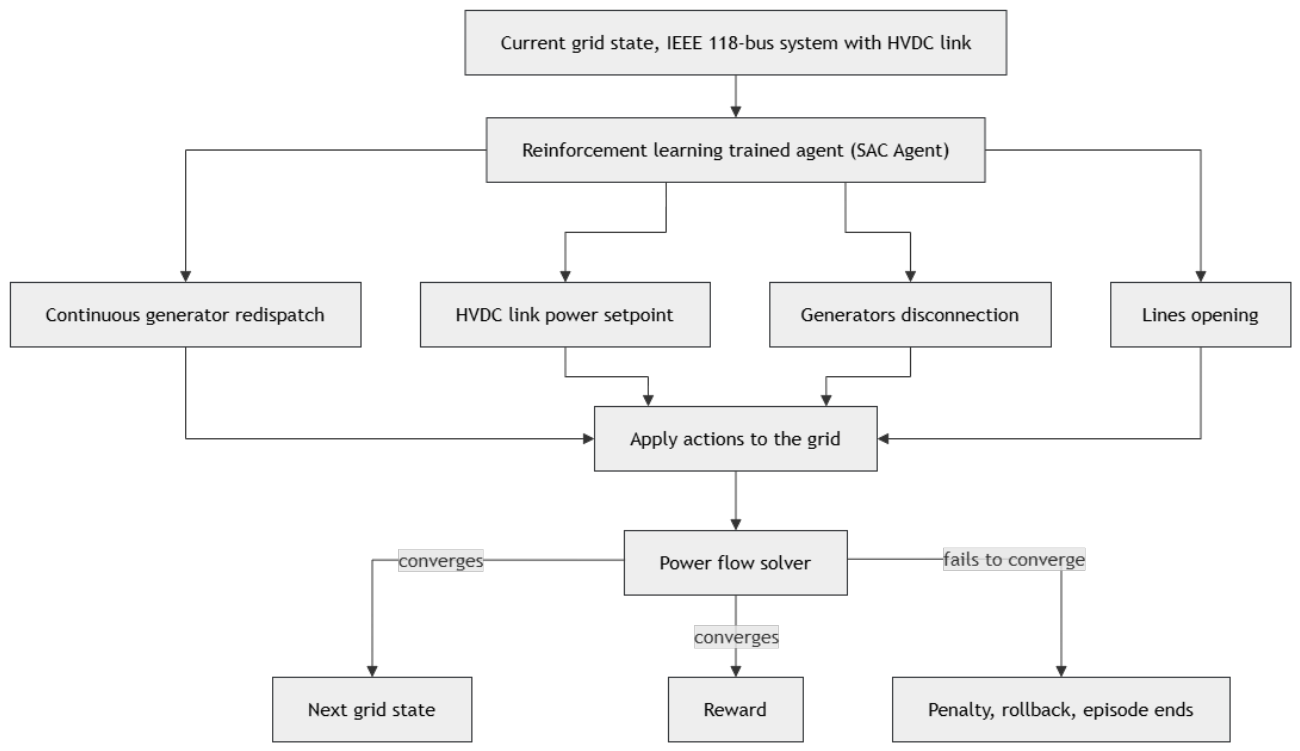
Figure 2.
Critic and actor losses of the hybrid SAC agent over environment steps (seed 42). (a) Critic loss, on a logarithmic scale; its upward drift in the second half of the run motivates the checkpoint selection protocol. (b) Actor loss.
Figure 2.
Critic and actor losses of the hybrid SAC agent over environment steps (seed 42). (a) Critic loss, on a logarithmic scale; its upward drift in the second half of the run motivates the checkpoint selection protocol. (b) Actor loss.
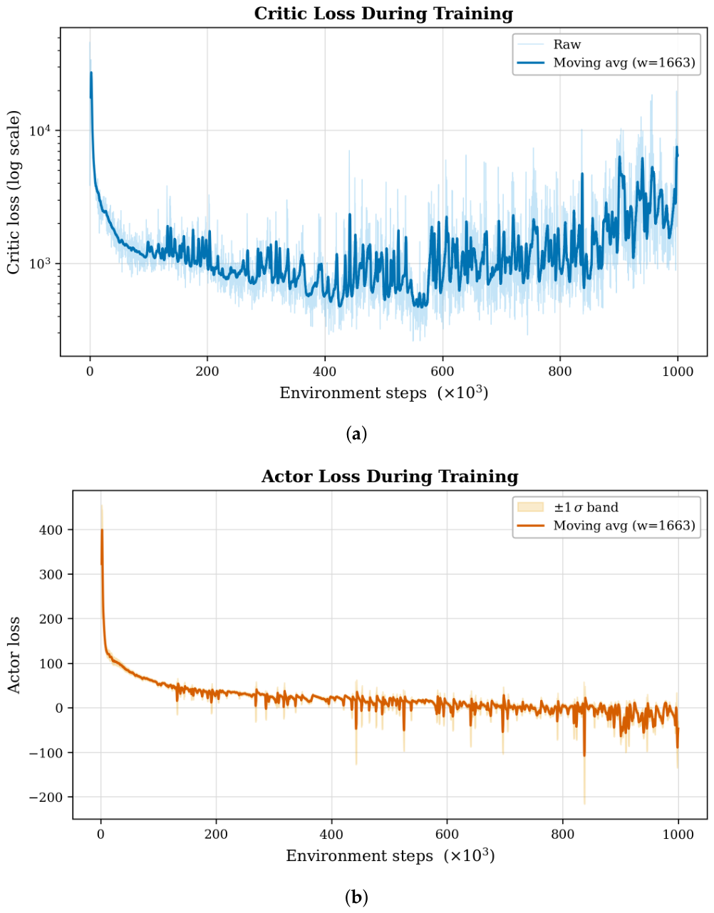
Figure 3.
Episode-level training metrics of the hybrid SAC agent on the AC IEEE 118-bus environment with VSC-HVDC. (a) Episode reward. (b) Redispatched power per episode.
Figure 3.
Episode-level training metrics of the hybrid SAC agent on the AC IEEE 118-bus environment with VSC-HVDC. (a) Episode reward. (b) Redispatched power per episode.
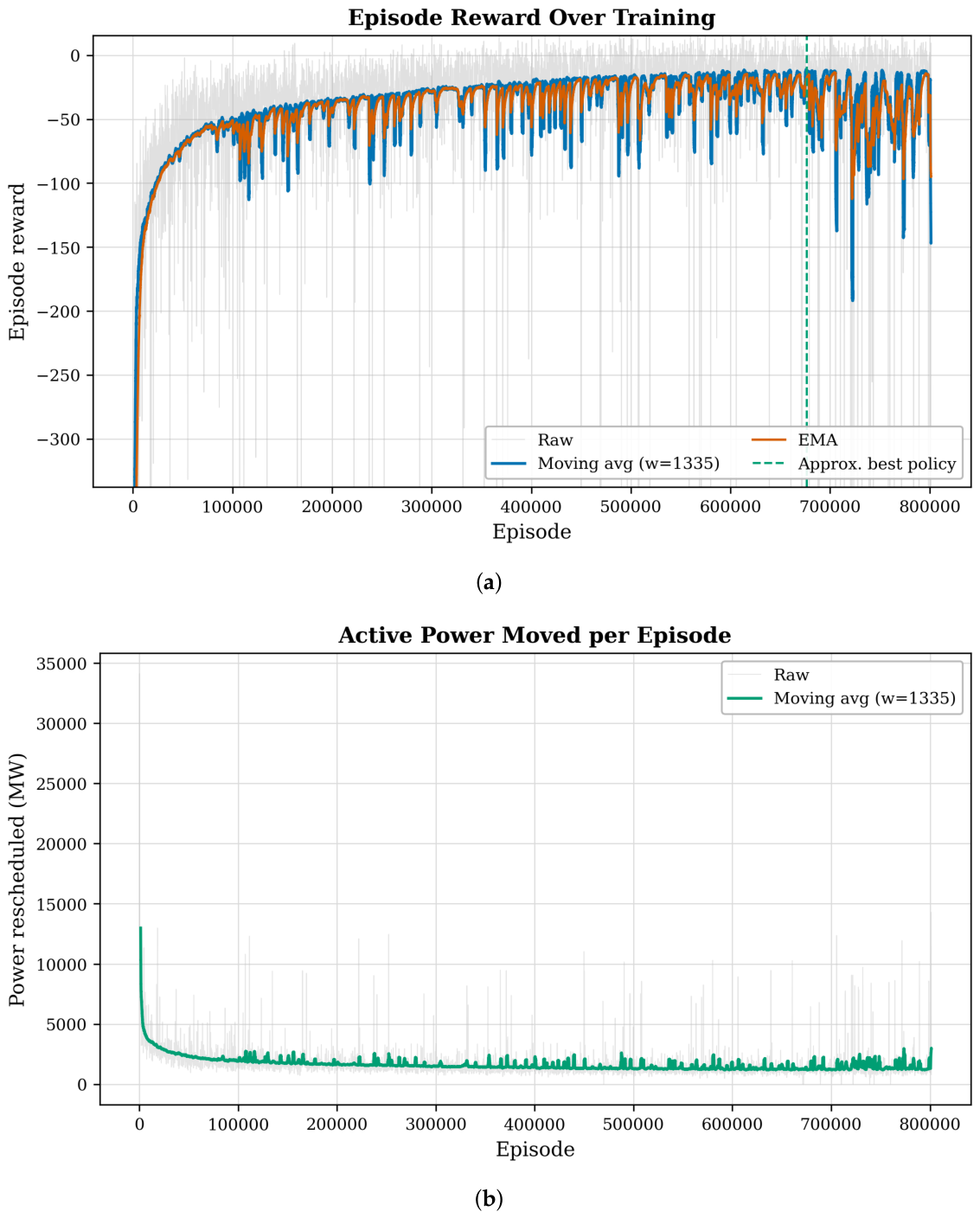
Figure 4.
Corrective action of the hybrid SAC agent on the AC IEEE 118-bus system [31] with VSC-HVDC [13]. (a) Initial overloaded state; branches drawn in red exceed their thermal rating (). (b) After the hybrid SAC action, every branch is within its thermal limit.
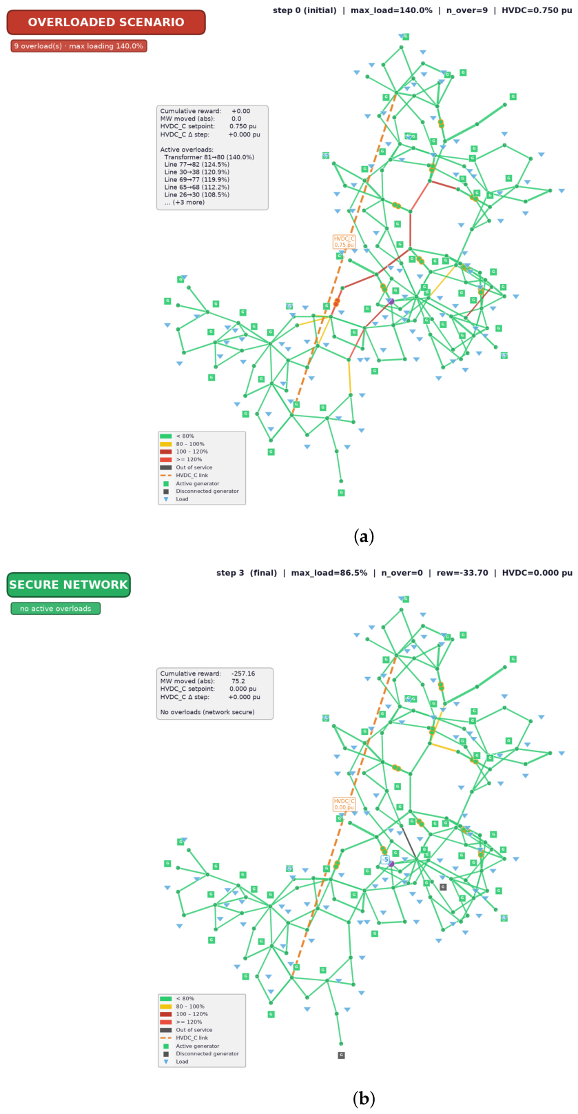

Table 1.
Composition of the 906-dimensional observation vector.
| Block | Content | Dim. | Clipping |
|---|---|---|---|
| Branch loading | / thermal rating | 186 | |
| Reactive flow | / thermal rating | 186 | |
| Generator active | 53 | ||
| Generator reactive | 53 | ||
| Branch status | 1 in service, 0 out of service | 186 | — |
| Candidate gen. status | availability of the 4 candidates | 4 | — |
| Voltage magnitude | 118 | ||
| Voltage angle | (rad) | 118 | |
| Slack power | normalised slack active power | 1 | |
| HVDC set-point | 1 | ||
| Total | 906 |
Table 2.
Hybrid SAC configuration.
| Hyperparameter | Value |
|---|---|
| Replay buffer size | 200,000 transitions |
| Warm-up (random) steps | 2000 |
| Batch size | 256 |
| Discount factor | 0.99 |
| Polyak coefficient | 0.005 |
| Learning rate (actor, critic, temperatures) | |
| Gradient updates per environment step | 1 |
| Target entropies | |
| clamps | , , |
| Gumbel temperature | , decay /step |
| Actor trunk | |
| Critic hidden layers (twin) | |
| Observation / action dimension | 906 / 73 |
| Episode step limit | 10 |
| Total training steps | |
| Device | multi-core CPU (no GPU) |
Table 3.
Performance on the evaluation sets. SR = success rate, that is, the fraction of scenarios in which every branch is returned to within its thermal rating. AC verification is the fraction of episodes whose final state is confirmed by an independent power flow solve. The two 500-scenario batches and the 1806-scenario corpus were run with checkpoints from different seeds, stated in the last column; the first two rows are therefore the ones to compare with each other.
Table 3.
Performance on the evaluation sets. SR = success rate, that is, the fraction of scenarios in which every branch is returned to within its thermal rating. AC verification is the fraction of episodes whose final state is confirmed by an independent power flow solve. The two 500-scenario batches and the 1806-scenario corpus were run with checkpoints from different seeds, stated in the last column; the first two rows are therefore the ones to compare with each other.
| Evaluation Set | Scen. | Solved | SR | Ini | Fin | Steps | AC Verif. | Seed, Ckpt. |
|---|---|---|---|---|---|---|---|---|
| 500, intact grid | 500 | 493 | 98.6% | 117.4% | 85.5% | 1.50 | 100.0% | 42, best |
| 500, up to 3 outages | 500 | 487 | 97.4% | 119.8% | 89.1% | 1.71 | 99.6% | 42, best |
| 1806, best checkpoint | 1806 | 1806 | 100.0% | 116.6% | 79.5% | — | — | 73, best |
| 1806, final checkpoint | 1806 | 1673 | 92.6% | 116.6% | 85.9% | — | — | 73, final |
Table 4.
Success rate on the 500-scenario batch with outages, by initial maximum loading and by number of simultaneous outages in the initial state.
Table 4.
Success rate on the 500-scenario batch with outages, by initial maximum loading and by number of simultaneous outages in the initial state.
| Initial Loading | Solved/Total | SR | Outages | Solved/Total | SR |
|---|---|---|---|---|---|
| 100–105% | 60 / 60 | 100.0% | 0 | 235 / 238 | 98.7% |
| 105–110% | 64 / 65 | 98.5% | 1 | 143 / 153 | 93.5% |
| 110–115% | 52 / 53 | 98.1% | 2 | 104 / 104 | 100.0% |
| 115–120% | 69 / 69 | 100.0% | 3 | 5 / 5 | 100.0% |
| 120–130% | 125 / 129 | 96.9% | |||
| 130–200% | 117 / 124 | 94.4% | |||
| Total | 487 / 500 | 97.4% | Total | 487 / 500 | 97.4% |
Table 5.
Behaviour of the policy on the 500-scenario batch with outages. The redispatched power is the sum of over the episode, recomputed with the environment’s own cost coefficient. The set-point change is measured between the start and the end of the episode; the per-action increment is bounded by .
Table 5.
Behaviour of the policy on the 500-scenario batch with outages. The redispatched power is the sum of over the episode, recomputed with the environment’s own cost coefficient. The set-point change is measured between the start and the end of the episode; the per-action increment is bounded by .
| Metric | Value |
|---|---|
| Episodes solved in a single step | 332 (66.4%) |
| Episodes solved in two steps | 116 (23.2%) |
| Episodes reaching the step limit | 13 (2.6%) |
| Mean steps per episode | 1.71 |
| Initial overloaded branches (mean / max) | 2.73 / 14 |
| Mean loading reduction | 24.86 pp |
| Mean redispatched power | 2537 MW |
| Mean episode reward | |
| Episodes in which the HVDC is modulated | 486 (97.2%) |
| HVDC set-point, mean initial / final | / |
| HVDC set-point change over episode, range | |
| Distinct lines switched by the agent | 4 (of 13 candidates) |
| Distinct branches congested in the batch | 70 |
Table 6.
Training runs. SR, run mean is the success rate averaged over every episode of the run; SR, final window is the mean over the last 100 episodes only, the short rolling statistic used for checkpoint selection. The two are not comparable, and the second is noisy by construction. Run means are not available for the 200,000-step pilot.
Table 6.
Training runs. SR, run mean is the success rate averaged over every episode of the run; SR, final window is the mean over the last 100 episodes only, the short rolling statistic used for checkpoint selection. The two are not comparable, and the second is noisy by construction. Run means are not available for the 200,000-step pilot.
| Seed | Steps | Episodes | Wall Clock | SR, Run Mean | SR, Final Window |
|---|---|---|---|---|---|
| 42 | 801,284 | 1204 min | 0.9820 | 0.88 | |
| 43 | 802,480 | 1531 min | 0.9821 | 0.32 | |
| 73 | 757,418 | 1523 min | — | 0.87 | |
| 74 | 166,703 | 233 min | — | 1.00 |
Table 7.
Ablation study, reproduced from the extended work [32]. Each row modifies one element of the reference configuration; the success rate is measured on the intact-grid batch.
Table 7.
Ablation study, reproduced from the extended work [32]. Each row modifies one element of the reference configuration; the success rate is measured on the intact-grid batch.
| Configuration | SR (%) | Final (%) | Steps/ep. |
|---|---|---|---|
| Reference configuration | 98.6 | 0.89 | 1.50 |
| Parallel DQN heads instead of GS-ST | 87.5 | 4.3 | 1.54 |
| Single entropy temperature | 94.0 | 1.8 | 1.38 |
| Without the fix in reset() | 71.0 | 11.2 | 2.10 |
Disclaimer/Publisher’s Note: The statements, opinions and data contained in all publications are solely those of the individual author(s) and contributor(s) and not of MDPI and/or the editor(s). MDPI and/or the editor(s) disclaim responsibility for any injury to people or property resulting from any ideas, methods, instructions or products referred to in the content. |
© 2026 by the authors. Licensee MDPI, Basel, Switzerland. This article is an open access article distributed under the terms and conditions of the Creative Commons Attribution (CC BY) license (http://creativecommons.org/licenses/by/4.0/).
Copyright: This open access article is published under a Creative Commons CC BY 4.0 license, which permit the free download, distribution, and reuse, provided that the author and preprint are cited in any reuse.