

Submitted:
18 August 2026
Posted:
20 August 2026
You are already at the latest version
Abstract
Understanding how visual exploration evolves over time during complex decision making remains challenging, as the dynamics of underlying cognitive processes are difficult to observe. Hidden Markov models are widely used to model eye movement sequences, but their assumption of stationary transition probabilities limits their ability to identify successive phases. This study investigated whether Switching Hidden Markov Models (SHMMs), trained only on fixation positions, could segment visual exploration during an obstacle-avoidance task requiring a left/right decision. Individual SHMMs with two or three high-level (HI) states were trained without using reaction times. HI states were characterized through transition-matrix variability, saliency maps, cumulative dwell times in regions of interest, and their association with reaction times. Both models produced temporal segmentations consistent with decision making. Early HI states showed greater interindividual variability and exploration focused on obstacles, whereas later states were more homogeneous and reflected decision confirmation followed by reorientation toward the center of the screen. The transition to the final HI state of the three-state model best predicted reaction time. Furthermore, cumulative log-likelihood significantly improved this prediction, indicating that SHMM confidence provided complementary behavioral information. These findings show that SHMMs trained only on fixation positions can identify phases consistent with the organization of the decision-making process, including early evidence accumulation and late decision confirmation.
Keywords:
Switching Hidden Markov Model
; eye movement
; decision making
1. Introduction
Hidden Markov chains [1] are commonly used in eye tracking to segment scan paths into homogeneous phases based on the statistical properties of eye movements. When fixation positions are used as observations, the hidden states correspond to regions of interest (ROIs) defined by recurrent fixation locations, while the transition matrices capture how these ROIs are visited over time [2,3].
Two previous studies [4,5] have demonstrated that Hidden Markov Models (HMMs) can account for inter-individual spatio-temporal variability during a face recognition task when applied to eye movements. Through unsupervised learning, these models have revealed two distinct classes of exploration profile among participants, depending on their cognitive style: holistic versus analytic [6]. However, these models assume that transition probabilities between ROIs remain stationary throughout the trial. This assumption may be challenged in complex tasks involving multiple successive cognitive phases, each of which is potentially associated with a distinct visual exploration pattern [7]. Indeed, research on decision-making has shown that eye movement behaviors evolve over time as participants gather, integrate, and verify relevant information for the decision [8,9]. In this context, it is worth considering that the different phases of a single task may be associated with distinct visual exploration dynamics.
To address this limitation, Switching Hidden Markov Models (SHMMs) enable the simultaneous modeling of low-level hidden states (i.e., ROIs) and higher-level hidden states (HIs), as proposed by Chuk and collaborators (2020). Although HI states share the same ROIs, they are characterized by distinct transition matrices. Therefore, SHMMs are particularly well-suited to modeling continuous cognitive phase shifts within a single task.
Olivier and collaborators (2022) also demonstrated that hidden semi-Markov models [11] can perform unsupervised temporal segmentation into interpretable cognitive phases by explicit-ly accounting for statistical state-duration distributions. The researchers applied this approach to a text-reading task in which participants had to decide whether a previously presented theme was semantically related to the text’s content as they read. The model did not directly analyze fixation positions. Instead, it focused on transitions between fixations (saccades). To achieve this, a preprocessing step was applied, which associated each fixation with the closest word or group of words in the text. Then, a categorical variable representing the type of transition of each saccade ("backward" and "forward" with two different spans, and "re-fixation") was used as the observed data. In this context, the semi-Markov models were based on variables observed beyond raw data (such as fixations or saccades), since these were enriched with information from the text’s words.
Using a similar approach, our study aimed to evaluate the ability of a SHMM to segment the scanpaths produced during a complex visual exploration and decision-making task. Inspired by the aeronautical domain, the experimental task involved monitoring the movement of an autonomous drone among obstacles simulating air traffic. Participants had to decide which direction the drone should move to best avoid obstacles. The relatively long duration of the presentation of successive obstacles allowed participants to go through multiple successive stages of the decision-making process, from gathering initial information to preparing and executing the response, and potentially verifying it.
We chose to use SHMM because they can identify both low-level states (i.e., ROIs) and high-level states (high-level features, HIs) through unsupervised learning without the need for any prior ROI classification. SHMMs were particularly well suited for our study because they can capture the complex temporal dynamics of scanpaths without requiring prior annotation, which is a challenging task in the context of complex decision-making. SHMM also able cognitive interpretation of the identified states [2]. Therefore, we used eye fixation positions as the model’s sole observations. The primary goal of this approach was to determine whether an SHMM could identify shifts in visual exploration dynamics corresponding to different phases of cognitive processing in the context of a complex visual exploration and decision-making task in a fully unsupervised manner.
Given the exploratory nature of this study, we hypothesized that a SHMM with two or three high-level states could segment scanpaths into interpretable temporal phases despite substantial inter-individual variability. Specifically, we expected the identified states to align with the decision-making process and to exhibit distinct properties in terms of: (i) transition dynamics be-tween ROIs, (ii) spatial distribution of fixations, and (iii) relationship with reaction times, even though the latter were not used during model training.
2. Materials
2.1. Participants
Fifty-six participants took part in the experiment (38 females, M = 22 years, SD = 4.2 years). Three participants were excluded from the sample due to a misunderstanding of the instructions or early termination. All participants had normal or corrected vision, no history of psychiatric or neurological disorders before or during the experiment, and were not taking any medication that could affect the nervous system. Participants provided written informed consent and were compensated with €90 for their participation. This research was approved by the Ethics Committee (Comité de Protection des Personnes Nord Ouest IV, reference no. 38RC24.0131).
2.2. Design
Participants completed three experimental sessions (Session 1: Actor; Sessions 2 and 3: Supervisor), spaced approximately nine days apart. While all three sessions were part of a larger project, this study only analyzed the eye-tracking and behavioral data from the first session (Actor), in which participants were required to make active decisions. The session included four blocks of 32 trials each, for a total duration of approximately 60 minutes. A 32-trial training phase (10 minutes) preceded it. A debriefing was conducted at the end of the final session, during which the experimental conditions and study objectives were explained. All sessions were performed at the IRMaGe Neurophysiology facility (Grenoble, France).
2.3. Procedure
The experimental task involved actively exploring a dynamic scene leading to a decision-making process. In an aeronautical supervision context, participants were required to supervise an autonomous drone that was always positioned at the center of a radar. Obstacles representing air traffic moved from the top to the bottom of the screen relative to the drone. The drone was equipped with an obstacle-avoidance system that was designed to detect obstacles and autonomously select one of two invariant avoidance trajectories: left or right. The system had a 25% error rate. During this session, similar to the drone’s control system, participants had to explore the scene containing moving obstacles and decide which direction to take to avoid them (left or right). They had to make this decision during the exploration phase. The chronological sequence of a trial is illustrated in Figure 1.
A trial began with an Initialization phase (2,400 ms) during which no obstacles were presented. The following Conflict phase (6,600 ms) involved the progressive appearance of obstacles from the top of the screen (see the Materials section for a description of the stimuli). During this phase, participants were instructed to indicate the avoidance trajectory the drone should follow (left or right) by pressing a response key as quickly as possible while minimizing errors.
During the System Decision phase (1,000 ms), the system’s response was displayed in the center of the screen as a colored arrow. Then, the Validation phase began when the central circle around the drone turned blue; participants had to press a response key to valid the system’s decision if they deemed it correct.
Finally, the Avoid phase (14,500 ms) started when the central circle around the drone turned white. This phase simulated the drone’s movement along its chosen trajectory or the trajectory corrected by the participant. It thus allowed them to visualize the avoidance path among the obstacles. At the end of each trial, the participant was required to fixate on a circle appearing in the center of the screen. This allowed the experimenter to apply a drift correction or recalibration, if necessary.
A total of 128 trials were presented to participants, divided into four blocks of 32 trials each. For half of the trials (random order), the correct avoidance trajectory was to the left, and for the other half, it was to the right. Additionally, the system’s decision was incorrect in 25% of the trials (random order). Before the first session, participants completed a 32-trial training phase to learn the two possible symmetrical trajectories with respect to the vertical midline of the screen. The training trials followed the same temporal sequence of phases as previously described. Only the Avoid phase was replaced with:
- Feedback on the participant’s responses (2,000 ms), concerning both the direction decision and validation;
- A visualization phase of the chosen trajectory (2,500 ms), allowing participants to identify the positions of obstacles on or near the trajectory, i.e., those relevant to decision-making, for each trial.
Although eye movements and EEG activity were simultaneously recorded during the experiment, the present study only focused on the analysis of eye-tracking data. EEG data will be the subject of specific analyses in future work. For this study, we therefore analyzed only eye-tracking data (eye fixations) and behavioral data (decision to choose the avoidance trajectory: left or right) during the Conflict phase.
A photodiode placed on the screen detected a light appearing at the beginning of each of the five phases segmenting a trial. Upon each detection, a trigger was sent to the eye tracker via its parallel port to precisely measure the start and end of each phase.
The experiment was programmed in TypeScript and executed in a Node.js environment. Communication with the eye tracker was handled by a dedicated Python module, called from Node.js using the node-calls-python library [12]. Data exchange between the Node.js server, the eye tracker, and the graphical interface was implemented using the WebSocket protocol, via the ws library [13]. This was an adaptation of the program used by Salomone et al. (2026).
2.4. Visual Stimuli
The visual scene consisted of:
- a drone was represented in a central circle (radius 1°), fixed at the center of the screen,
- obstacles, depicted as yellow triangular shapes within a circle (radius 0.45°), descending vertically from the top of the screen toward the drone,
- a neutral background, representing a stylized radar, with fixed speed and altitude information to avoid visual distractions.
The 18 obstacles were horizontally distributed: six on the left, six in the middle, and six on the right. The minimum distance between two adjacent obstacles was 2.2°. Their positions were updated at a frequency of 30 Hz.
During trial, among the six obstacles located on the left or right of the drone’s trajectory, one, two or three reached their final positions, either on the trajectory or very close to it. For example, if these obstacles were on the right side, it would indicate that the left trajectory should be chosen to avoid them. These obstacles were relevant for determining whether the system’s avoidance decision (left or right) was correct. During the first 3,600 ms, the obstacles appeared progressively and decelerated until reaching near-zero speed. At this moment, all obstacles were present and almost stationary. This configuration was maintained for the following 3,000 ms, until the end of the Conflict phase. From the drone’s perspective, this obstacles’ change in speed simulated a deceleration as the drone approached them
An example video (Trial.mp4) illustrating this scene for a trial is available via this link.
2.5. Apparatus
Each dynamic stimulus was displayed on a 27-inch screen with a resolution of 1920 × 1080 pixels and a refresh rate of 60 Hz. Participants were seated 60 cm from the screen. The stimuli covered a visual angle of 34.6° × 28.4°.
Eye position on the screen was recorded using an Eye-Link 1000 binocular infrared eye tracker with a sampling rate of 1,000 Hz. For each participant, the eye used for analysis was selected during the setup phase based on the pupil detection stability and the quality of the calibration-validation process. Calibrations were accepted when the average validation error was below 1° of visual angle and the maximum error was below 1.5°.
The Eyelink software automatically detected saccades and fixations using three distinct thresholds: a minimum displacement of 0.1° from the previous eye position, a minimum velocity of 30°/s, and a minimum acceleration of 8,000°/s². A 9-point calibration was performed before the task and repeated during the blocks when necessary.
2.6. Behavioral Data
The behavioral data analyzed included the reaction time for deciding to choose the avoidance side and the response itself (left or right).
2.7. Eye-Tracking Data
The start times, end times, and positions of eye fixations were obtained from the automatic extractions performed by the eye tracker. To prepare the SHMM learning based on eye fixation positions during the Conflict phase, each fixation position was classified into one of the following four categories:
- Center (within a 6° × 6° square at the center of the screen, area without obstacles and location of the system’s feedback during System Decision and Validation phases),
- Bottom (below a horizontal line extending across the full width of the screen and aligned with the lower edge of the previously described Center square, area without obstacles),
- Out (outside the screen),
- Obstacle (all other fixations).
Fixations in the Obstacle region contributed to task resolution because they were located in the part of the visual scene containing the moving obstacles. The Center region was particularly relevant to the task because the system’s choice for the avoidance side was displayed there. Fixations in the Bottom and Out regions were non-informative for task resolution, and did not contribute to SHMM learning.
3. Methods
3.1. Switching Hidden Markov Model
3.1.1. Learning
Switching Hidden Markov Models (SHMM) were used to model the participants’ eye movement behavior during the Conflict phase. To capture inter-individual variability, an SHMM was learned for each participant based on trials that:
- had valid synchronization of photodiode markers,
- were correctly solved by the participant,
- contained more than three fixations.
This choice was consistent with the work of Chuk et al. (2014) which showed that the transition dynamics between regions of interest differed primarily between eye movement patterns associated with correct and incorrect responses. Including both correct and incorrect trials could have introduced additional heterogeneity in the estimation of transition matrices. Among the selected trials, the first fixation which was not informative for the task, as well as fixations classified as Bottom and Out, were excluded.
Since the obstacles moved from top to bottom and the task was to decide which side to avoid, the vertical position of the fixations was not considered. Therefore, the input data were one-dimensional, computed from the horizontal positions of the fixations. For trials in which the correct side was the left side (an arbitrary choice), these positions were transformed by mirror symmetry relative to the center of the screen. This transformation allowed all trials to be grouped together, by considering the correct side to always be the left. Additionally, to distinguish between fixations classified as Center and Obstacle after reduction to a single horizontal dimension, the horizontal positions of fixations classified as Center were offset by a constant to obtain negative values.
Two learning configurations were tested:
- R = 4 low-level states (denoted ROI, Regions Of Interest);
- S = 2 or S = 3 high-level states (HI).
Hereinafter, the HI states were denoted by HIn_S, where n ranges from 1 to S and S = 2 or S = 3.
For each configuration, a SHMM was learned for each participant based on their one-dimensional fixation positions. The initialization and configuration parameters were identical for all learning processes. They are summarized in Table 1.
These prior probabilities and initial transition matrices constrained the initial HI state to be the first (HI1_2 or HI1_3), and the order of HI state visits was strictly increasing, with no possibility of returning to a previous state. Thus, at most one transition between adjacent HI states could occur during a trial. This allowed to define a unique transition time between adjacent HI states for each trial. These transition times are denoted as follows:
- THI12_2 for the SHMMs with S = 2,
- THI12_3 and THI23_3 for the SHMMs with S = 3.
The SHMMs were implemented in MATLAB using the toolbox developed by Chuk et al. (2020). After learning, the estimated parameters for each model were obtained:
- prior probabilities and transition matrices for HI and ROI states,
- parameters of Gaussian distributions of observations (means and variances) for ROI states,
- global log-likelihood of the model.
3.1.2. SHMM Standardized Representation and States Restoration
After learning the SHMMs, a standardization step was applied to ensure consistent naming of HI states and ROIs across participants. The HI states were numbered in descending order of their prior probabilities, and the ROIs were ordered in ascending order of their one-dimensional positions. After standardization, ROI 1 corresponded to the Center area (negative position), and the other three ROIs were ordered from left (correct avoidance side after mirror transformation) to right (incorrect side).
The Viterbi algorithm was then used to restore the combined ROI × HI sequence for each trial. The cumulative log-likelihood of restoration (Cml) was calculated and used as an indicator of segmentation quality. The consistency of the HI state standardization was verified by ensuring that the transition times between adjacent states were in ascending order. Finally, experimental saliency maps were generated for each HI state using the two-dimensional positions of the original fixations [15,16]. The maps were obtained by convolution with a Gaussian kernel with a standard deviation of 2°.
3.2. Linear Mixed-Model Analyses of Participant-Level Measures
For analyses based on participant-level means, statistical inference was performed using Linear Mixed Models (LMMs). For each analysis, two models were compared: one including a random intercept for participant and one without random effects. Whether the random intercept improved model fit was assessed using the Akaike Information Criterion (AIC), and the most parsimonious model was retained.
LMMs were implemented in MATLAB using the fitlme() function and estimated by maximum likelihood. Fixed effects were evaluated using marginal F-tests. Planned pairwise comparisons were performed by testing linear contrasts of the fitted model coefficients (coefTest() function) with Bonferroni correction for multiple comparisons. Effect sizes were quantified using partial eta-squared (η2p). Model assumptions were assessed by inspecting the residuals of the final model, including their distribution, conditional independence, and homogeneity of variance.
3.3. Transition Times Between HI States
To evaluate the behavioral relevance of the segmentation produced by the SHMMs, we examined the relationship between the transition times of high-level states (HI) and reaction times (RT). Since RTs were not used during learning, this analysis tested whether the temporal segmentation estimated from fixation positions alone could predict the observed behavior, and thus confirm the interpretation of our HI states.
Three transition times were considered: the THI12_2 transition from the two-state model (S = 2), as well as the THI12_3 and THI23_3 transitions from the three-state model (S = 3). Two complementary approaches were applied to each of these transitions.
First, the gap between the SHMM-estimated transition time and the observed RT was computed for each trial to evaluate the temporal proximity between the SHMM segmentation and the observed behavior directly. The absolute value of the gap was analyzed using LMMs with transition (THI12_2, THI12_3, and THI23_3) as a fixed effect.
Second, the relationship between RT and transition times was evaluated. Unlike the previous analyses, which were performed on participant-level means, the relationship between transition times and RT was analyzed at the trial level using LMMs. For each transition time, we compared three models of increasing complexity:
- a fixed-effects-only model,
- a model including a random intercept per subject,
- a model including both a random intercept and a random slope per subject.
The models were compared using the Akaike Information Criterion (AIC), log-likelihood, and adjusted coefficient of determination (R²). The model with the best trade-off between fit quality and parsimony was retained. Finally, the cumulative log-likelihood of the Viterbi state restoration (Cml) was added as an additional predictor to evaluate whether the confidence of the SHMM segmentation provided complementary information for explaining RT.
The tested hypotheses were as follows:
- If the transitions detected by the SHMM are linked to RTs, then it suggests that HI states reflect the relevant behavioral stages of the decision-making process.
- If the Cml variable improves the explanation of RTs, then it suggests the trials that are better described by the SHMM exhibit a more consistent temporal organization.
3.4. Dwell Times During States
The Kullback–Leibler (KL) divergence was used for two purposes:
- To characterize the transitional state HI2_3 from the SHMM with three HI states. This is an intermediate state between HI1_3 and HI3_3.
- To assess inter-individual variability in the HI state representations.
For each SHMM, each HI state was characterized by a 4×4 transition matrix (R = 4), which reflected the transition probabilities between ROIs (low-level states) during that HI state. The KL divergence, which measures the dissimilarity between probability distributions, was used here to quantify the differences between these matrices. Each row of this matrix difference represents a probability distribution over ROIs. The KL divergences were transformed using a Box–Cox transformation [17] with a common λ parameter to approximate a normal distribution across all distributions. The λ parameter was then determined to optimize global normality across all conditions.
3.4.1. Intermediate State HI2_3 Obtained from SHMMs with 3 HI States
To characterize the role of the intermediate state HI2_3 in the exploration dynamics, we compared its transition matrix with those of the other two states obtained from SHMMs with three HI states, namely HI1_3 and HI3_3 using KL divergence. Comparing these KL divergences allowed us to determine whether this intermediate state was closer to the dynamics of evidence accumulation (HI1_3) or confirmatory exploration (HI3_3). After a Box-Cox transformation, KL Divergence between HI2_3 and HI1_3, and between HI2_3 and HI3_3 were analyzed using LMMs with HI state (HI1_3, HI3_3) as a fixe effect.
The same methodology was applied to compare the intermediate state HI2_3 with the two states HI1_2 and HI2_2 obtained from SHMMs with two HI states.
3.4.2. Variability of Transition Matrices
Interindividual variability of HI states was assessed by analyzing the transition matrices between ROIs for each of the five HI states (HI1_2, HI2_2, HI1_3, HI2_3, and HI3_3), which were obtained from individual SHMMs with two and three HI states. For each HI state, the KL divergence was computed between the transition matrix of that HI state for each participant and the average transition matrix for that HI state across all participants. Thus, this divergence quantified the difference between the individual representation and the average representation of the HI state. This approach allowed us to quantify the inter-individual variability in how individual SHMMs characterized each HI state.
To analyze the variability of HI state representations, informed by KL divergences, we used LMMs after applying a Box–Cox transformation.
The transformed KL divergences were analyzed using LMMs with HI state (HI1_2, HI2_2, HI1_3, HI2_3, and HI3_3) as a fixed effect.
4. Results
4.1. Number of Trials and Fixations and Reaction Time
Participants correctly solved 92.9% of the trials (SE = 1.27). After applying the inclusion criteria, an average of 117.5 trials per participant (SE = 1.68) were retained for each SHMM learning. Retained trials contained an average number of 16.4 fixations (SE = 0.33), of which an average of 14.9 fixations (SE = 0.33) contributed to SHMM learning.
The mean reaction time (RT) was 3,192.4 ms (SE = 135.59).
4.2. Experimental Saliency Maps for Each HI State
The experimental saliency maps for each HI state are illustrated in Figure 2. After standardization, the four ROIs were ordered by increasing 1D position: ROI 1 to ROI 4. For interpretability, they were renamed as follows: ROI 1 = Center (negative 1D position, corresponding to the drone’s location), ROI 2 = ValidSide (left, the correct avoidance side after the mirror transformation), ROI 3 = Middle (the intermediate area between ValidSide and WrongSide), and ROI 4 = WrongSide (right, the incorrect avoidance side after the mirror transformation).
Based on these maps, several observations were drawn:
- In the early states (HI1_2, HI1_3, and HI2_3), exploration primarily occurred in the ValidSide, Middle, and WrongSide ROIs. Moreover, participants fixated on the ValidSide ROI more often.
- During the later states (HI2_2 and HI3_3), exploration primarily occurred in the Center ROI, while exploration between the ValidSide and WrongSide ROIs continued.
To validate these spatial patterns, statistical analyses of cumulative dwell times across HI states and ROIs were conducted, as described in the following section.
4.3. Characterization of HI States by Cumulative Dwell Times in Low-Level States (ROI)
A LMM was used to analyze the effect of the high-level states (HI) and the low-level states (ROI) on the cumulative dwell time. For both model configurations (S = 2 and S = 3), model comparison showed that including a random intercept for participant did not improve model fit (an increase in AIC of 2.00 in both cases). Therefore, the fixed-effects-only models were retained for the subsequent analyses.
4.3.1. SHMM with two HI States
The main effect of the HI state (HI: HI1_2, HI2_2) was significant (F(1, 415) = 273.49, η2p = 0.40, p < 0.0001), with a longer cumulative dwell time in HI2_2 (1222.20 ± 30.64 ms) than in HI1_2 (879.70 ± 32.61 ms) (Figure 3a).
The main effect of the low-level state (ROI: Center, Middle, ValidSide, WrongSide) was also significant (F(3, 415) = 18.43, η2p = 0.12, p < 0.0001) (Figure 3b). Post-hoc comparisons with Bonferroni correction revealed that the cumulative dwell time in the Center ROI was significantly longer (1309.67 ± 74.50 ms) than in the ValidSide ROI (1195.83 ± 36.77 ms, F(1, 415) = 55.01, p < 0.0001), the Middle ROI (837.20 ± 42.09 ms, F(1, 415) = 16.40, p < 0.001), and the WrongSide ROI (856.91 ± 24.73 ms, F(1, 415) = 16.86, p < 0.001). Notably, the cumulative dwell time in the ValidSide ROI (1195.83 ± 36.77 ms) was significantly longer than in the Middle ROI (837.20 ± 42.09 ms, F(1, 415) = 11.34, p < 0.01) and the WrongSide ROI (856.91 ± 24.73 ms, F(1, 415) = 10.96, p < 0.01).
The HI × ROI interaction was significant (F(3, 415) = 76.02, η2p = 0.35, p < 0.0001), indicating that the effect of the low-level state (ROI) on the cumulative dwell time depended on the HI state (Figure 3c). Specifically, in HI1_2, the cumulative dwell time in the Center ROI (497.17 ± 104.43 ms) was significantly shorter than in the ValidSide ROI (1226.00 ± 80.06 ms, F(1, 415) = 55.01, p < 0.0001), the Middle ROI (895.12 ± 70.41 ms, F(1, 415) = 16.40, p < 0.001), and the WrongSide ROI (900.64 ± 41.78 ms, F(1, 415) = 16.86, p < 0.001). In contrast, in HI2_2, the cumulative dwell time in the Center ROI (2122.20 ± 90.16 ms) was significantly longer than in the ValidSide ROI (1165.70 ± 53.22 ms, F(1, 415) = 147.07, p < 0.0001), the Middle ROI (777.11 ± 56.45 ms, F(1, 415) = 156.57, p < 0.0001), and the WrongSide ROI (813.18 ± 34.17 ms, F(1, 415) = 151.86, p < 0.0001). Notably, while the cumulative dwell time in the ValidSide ROI (1226.00 ± 80.06) was significantly longer than in the WrongSide ROI during HI1_2 (900.64 ± 41.78 ms, F(1, 415) = 10.96, p < 0.05), these two times did not differ during HI2_2 (1165.70 ± 53.22 ms vs. 813.18 ± 34.17 ms, p = 1.00). The interaction effect was primarily driven by the Center ROI, for which the cumulative dwell time during HI2_2 (2122.20 ± 90.16 ms) was significantly longer than during HI1_2 (497.17 ± 104.43 ms, F(1, 415) = 273.49, p < 0.0001).
4.3.2. SHMM with Three HI States
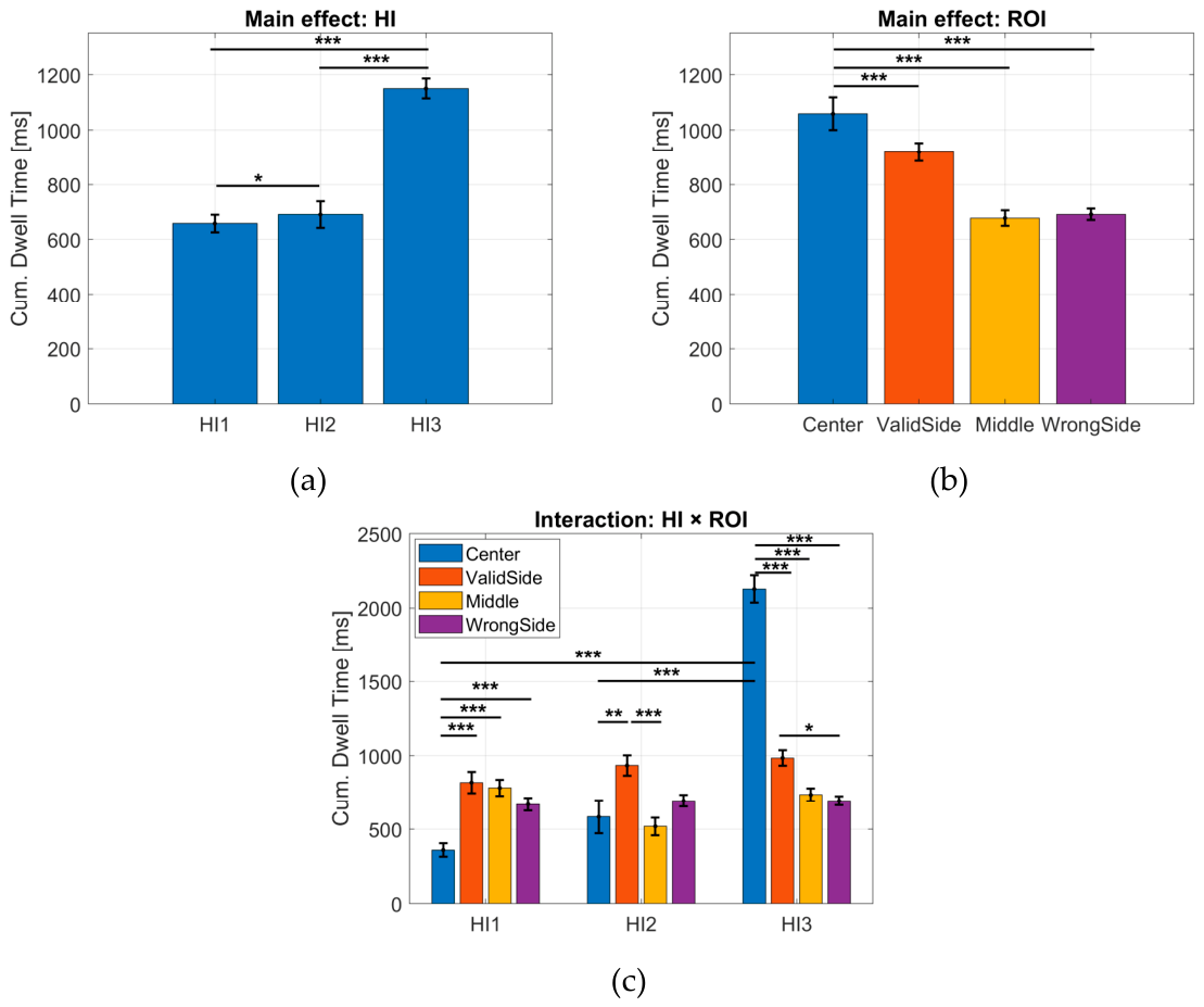
The main effect of the high-level state (HI: HI1_3, HI2_3, HI3_3) was significant (F(2, 602) = 233.30, η2p = 0.44, p < 0.0001). Post-hoc comparisons with Bonferroni correction showed that the cumulative dwell time in HI3_3 (1150.62 ± 35.62) was significantly longer than in HI2_3 (690.97 ± 48.76 ms, F(1, 602) = 281.6, p < 0.0001) and HI1_3 (658.34 ± 32.08 ms, F(1, 602) = 281.6, p < 0.0001). Additionally, the cumulative dwell time in HI1_3 (658.34 ± 32.08 ms) was significantly shorter than in HI2_3 (690.97 ± 48.76 ms, F(1, 602) = 5.8845, p < 0.05).
The main effect of the low-level state (ROI: Center, Middle, ValidSide, WrongSide) was also significant (F(3, 602) = 11.02, η2p = 0.05, p < 0.0001). Post-hoc comparisons with Bonferroni correction showed that the cumulative dwell time in the Center ROI was significantly longer (1059.11 ± 59.00 ms) than in the ValidSide ROI (919.58 ± 32.39 ms, F(1, 602) = 26.64, p < 0.0001), the Middle ROI (678.09 ± 28.48 ms, F(1, 602) = 22.83, p < 0.0001), and the WrongSide ROI (691.86 ± 21.18 ms, F(1, 602) = 12.24, p < 0.01).
The HI × ROI interaction was significant (F(6, 602) = 55.67, η2p = 0.36, p < 0.0001), indicating that the effect of the low-level state (ROI) on the cumulative dwell time depended on the high-level state. Specifically, in HI1_3, the cumulative dwell time in the Center ROI (359.42 ± 44.69 ms) was significantly shorter than in the ValidSide ROI (818.97 ± 72.27 ms, F(1, 602) = 26.64, p < 0.0001), the Middle ROI (782.90 ± 54.76 ms, F(1, 602) = 22.83, p < 0.0001), and the WrongSide ROI (669.48 ± 42.72 ms, F(1, 602) = 12.24, p < 0.05). In HI2_3, the cumulative dwell time in the ValidSide ROI (934.38 ± 69.30 ms) was significantly longer than in the Center ROI (583.66 ± 112.03 ms, F(1, 602) = 14.00, p < 0.01) and Middle ROI (519.05 ± 59.73 ms, F(1, 602) = 21.11, p < 0.001), while the dwell time in the ValidSide ROI (934.38 ± 69.30 ms) did not differ from that in the WrongSide ROI (693.71 ± 39.39 ms, p = 0.25). Finally, in HI3_3, the cumulative dwell time in the Center ROI (2128.10 ± 92.34 ms) was significantly longer than in the ValidSide ROI (985.00 ± 53.01 ms, F(1, 602) = 167.97, p < 0.0001), the Middle ROI (735.40 ± 42.16 ms, F(1, 602) = 249.34, p < 0.0001), and the WrongSide ROI (693.84 ± 30.90 ms, F(1, 602) = 251.35, p < 0.0001). Notably, in HI3_3, the cumulative dwell time in the ValidSide ROI (985.00 ± 53.01 ms) was significantly longer than in the WrongSide ROI (693.84 ± 30.90 ms, F(1, 602) = 10.36, p < 0.05). As with the two-state SHMM, the interaction effect was primarily driven by the Center ROI, for which the cumulative dwell time during HI3_3 (2128.10 ± 92.34 ms) was significantly longer than in HI1_3 (359.42 ± 44.69 ms, F(1, 602) = 398.31, p < 0.0001) and HI2_3 (583.66 ± 112.03 ms, F(1, 602) = 281.60, p < 0.0001).
Figure 4.
Mean cumulative dwell time (± SE) obtained from the three-HI state SHMM showing (a) the main effect of HI state, (b) the main effect of ROI, and (c) the HI × ROI interaction. Bonferroni corrected p, * p < 0.05, ** p < 0.01, and *** p < 0.001.
Figure 4.
Mean cumulative dwell time (± SE) obtained from the three-HI state SHMM showing (a) the main effect of HI state, (b) the main effect of ROI, and (c) the HI × ROI interaction. Bonferroni corrected p, * p < 0.05, ** p < 0.01, and *** p < 0.001.
4.4. Interpretation of the HI2_3 State from the SHMM with Three HI States
The HI2_3 state obtained from the SHMM with three HI states was a transitional state between the first state (HI1_3) and the last state (HI3_3). Individual KL divergences were computed between the transition matrix of this transitional state (HI2_3) and those of the HI1_3 and HI3_3 states. These KL divergences were transformed using a Box–Cox transformation (λ = 0.5) to approximate a normal distribution (Shapiro–Wilk test, p > 0.05 for all states). These KL divergences were then compared using a LMM. According to the AIC criterion, the fixed-effects model was retained. The results showed that the KL divergence between HI2_3 and HI1_3 (6.55 ± 0.54) was significantly lower than the KL divergence between HI2_3 and HI3_3 (7.39 ± 0.48; F(1, 104) = 7.25, η2p = 0.06, p < 0.01). The same methodology was applied to the two HI states, HI1_2 and HI2_2, obtained from the SHMM with two HI states. The results showed that the KL divergence between HI2_3 and HI1_2 (4.54 ± 0.52) was significantly lower than the KL divergence between HI2_3 and HI2_2 (6.21 ± 0.48, F(1, 104) = 26.85, η2p = 0.20, p < 0.0001).
These results consistently suggest that the exploration dynamics during this transitional HI2_3 state were more similar to evidence accumulation dynamics than to confirmatory exploration dynamics.
4.5. Inter-Individual Variability of HI State Characterizations
Each HI state was characterized by a transition matrix between the four ROIs (R = 4). To assess the inter-individual variability of this HI state characterization, KL divergences were calculated between the individual transition matrix (of each participant) for a given HI state and the average transition matrix for that HI state across all participants. A high KL divergence value indicated that an individual’s representation was far from the group average, thus reflecting high inter-individual variability. The KL divergences were transformed using a Box–Cox transformation (λ = -0.5) to approximate a normal distribution (Shapiro–Wilk test, p > 0.05 for all states). These KL divergences were then compared using a LMM. According to the AIC criterion, the fixed-effects model was retained. The results showed a significant effect of the HI state (F(4, 260) = 11.52, η2p = 0.15, p < 0.0001). Post-hoc comparisons with Bonferroni correction revealed two state groups characterized by a significant inter-individual variability difference (Table 2):
- Group 1 (final states): Low inter-individual variability states: HI2_2 and HI3_3, without significant inter-individual variability difference between these states.
- Group 2 (early states): High inter-individual variability states: HI1_2, HI1_3, and HI2_3, without significant inter-individual variability difference between these states.
These results suggest that the final states (HI2_2 and HI3_3) were more homogeneous across individuals, whereas the early states (HI1_2, HI1_3, and HI2_3) exhibited greater variability, which may be related to differences in individual exploration strategies.
4.6. Analysis of Transition Times Between HI States
4.6.1. Gap Between Transition Times and Reaction Time (RT)
To assess the temporal accuracy of the segmentations estimated by the SHMMs, the difference between the SHMM-predicted transition time and the observed reaction time (RT) was calculated for all participants and trials. A negative gap indicated that the SHMM predicted an earlier transition than the RT, while a positive gap indicated a later transition. This analysis was conducted for the three transitions between HI states: THI12_2 (S = 2), THI12_3, and THI23_3 (S = 3). Descriptive statistics across all trials and participants were presented in Table 3. The gap distributions for the three transitions exhibited high standard deviations (between 1,442 ms and 1,711 ms), reflecting substantial variability across trials and participants. The skewness coefficients were close to 0 (between -0.21 and 0.04), suggesting approximately symmetric distributions, while the kurtosis coefficients were close to 3 (between 2.99 and 3.30), indicating distributions close to normality.
Statistical analyses were performed on the individual means of the absolute gap values per participant for each transition, to compare differences between transition types at the group level (Figure 5).
An LMM was used with the absolute gap as the dependent variable, the type of transition (THI12_2, THI12_3, and THI23_3). According to the AIC criterion, the fixed-effects model was retained. The effect of transition type on the absolute gap was significant (F(2, 156) = 8.31, p < 0.001). Post-hoc comparisons with Bonferroni correction showed that the absolute gap was significantly smaller for THI23_3 (1,215.40 ± 56.46 ms) than for THI12_2 (1,398.68 ± 70.69 ms, F(1, 156) = 5.98, p < 0.05) and THI12_3 (1,518.90 ± 84.40 ms, F(1, 156) = 16.39, p < 0.001). No significant difference was observed between THI12_2 and THI12_3 (F(1, 156) = 2.57, p = 0.3324).
The estimated THI23_3 transitions were significantly closer to the observed RTs than the other two transitions, suggesting better temporal precision for this transition in the SHMM with three HI states.
4.6.2. Statistical Fit of Reaction Time to Transition Times
Reaction time (RT) was separately fitted from each of the three transition times using LMMs of increasing complexity. The results are presented in Table 4.
The LMM including a random intercept and a random slope per participant showed the best compromise between fit quality and parsimony (lowest AIC and highest adjusted R²) for all three transitions (Figure 6). Consistently with the previous analysis, the THI23_3 transition best explained RT compared to the other two transitions. Adding an indicator of confidence in the SHMM segmentation, estimated by the log-likelihood of state restoration for each trial (Cml_3), as an additional explanatory variable to the best model for THI23_3 improved its fit: the adjusted coefficient of determination increased by 4%, the Akaike Information Criterion (AIC) decreased by 289, and the residual standard deviation decreased by 24 ms. For this model, the coefficient β₂ associated with the log-likelihood Cml_3 was -7.71 ± 0.87 (p < 0.0001), indicating that trials with higher SHMM confidence had lower RTs.
These results showed that the transition times predicted by the SHMMs explained a significant portion of the RT variance, up to 62.81% for the THI23_3 transition. Introducing a random intercept greatly improved the model fit, revealing substantial inter-individual variability in baseline RT levels, with some participants consistently responding faster than others. Adding a random slope provided a more modest improvement, suggesting that individual differences are more related to global decision speed than to the relationship between transition time and RT. Finally, the confidence variable Cml provided significant complementary information, further improving the quality of the fit.
5. Discussion
The aim of this study was to demonstrate how a Switching Hidden Markov Model (SHMM) can achieve a relevant spatio-temporal segmentation of a complex experimental task involving multiple cognitive processes and substantial inter-individual variability. The experimental task was contextualized in the aeronautical domain and involved monitoring the movement of an autonomous drone navigating obstacles simulating air traffic and gradually descending toward the drone. Based on their exploration of the obstacle configuration in each trial, participants had to decide as quickly as possible which side (left or right) the drone should take to avoid the obstacles while minimizing errors. Obstacles appeared progressively during each trial, allowing participants to build their decision incrementally as they explored the scene. This setup enabled them to verify information before responding and continue confirmatory exploration after providing their decision.
Eye fixation positions were used as observations to identify different spatio-temporal patterns of visual exploration. In this exploratory approach, we hypothesized that a SHMM with two or three HI states could segment scanpaths into interpretable cognitive phases that occur at time points consistent with reaction times, even though reaction times were not used during training. The results supported this hypothesis, as both the two- and three-HI state SHMMs produced segmentations that were consistent with the temporal organization of the decision-making process. Notably, the analysis of reaction times suggested the existence of cognitive phases of com-parable duration, with an average reaction time of 3,192.4 ms within the 6,600-ms obstacle presentation phase constituting the Conflict Phase.
Unlike Chuk et al. (2020), who trained separate SHMMs based on target lateralization, we applied a mirror transformation to the fixation positions relative to the vertical central axis of the screen. This allowed us to pool all trials into a single representational space, defining the left side as the correct side for all trials. This strategy normalized lateralization without altering the relevant cognitive information, and increased the effective sample size available for SHMM training. It also simplified the interpretation of low-level states because the ValidSide ROI always corresponded to the correct side and the WrongSide ROI always corresponded to the incorrect side after transformation.
The choice of a two-HI state configuration was consistent with the task structure, which in-volved an explicit decision-making process during visual exploration. Due to the substantial inter-individual variability associated with this type of task, we also tested a three-HI state con-figuration to determine whether the model would identify a more ambiguous intermediate stage. The HI states can be interpreted as successive stages of the decision-making process, ranging from an early phase dominated by information search to a later phase of decision verification and consolidation [18]. This interpretation aligns with the model structure, in which transitions are constrained to follow a forward temporal order, with no return to a previous HI state. This constraint was particularly well-suited to the task, during which relevant information appeared progressively, allowing participants to gradually consolidate their decision as they accumulated evidence.
The high accuracy rate (92.9%) demonstrated that participants reliably performed the task, which further supports the interpretation that HI states reflect effective decision-making processes.
Analyzing the inter-individual variability in HI states provided additional support for interpret-ing them as successive phases of the decision-making process. Calculating the Kullback-Leibler divergences between individual transition matrices and the average transition matrix for each state revealed two distinct groups: the final states of both models (HI2_2 and HI3_3) exhibited low inter-individual variability, whereas the early states (HI1_2, HI1_3, and HI2_3) were significantly more variable. These results suggest that participants employed more diverse visual strategies during the initial phases of information gathering and integration [8], before converging toward more homogeneous behaviors as the decision emerged [9,19]. For the three-state HI model, this interpretation was further supported by the analysis of the intermediate state (HI2_3), whose dynamics appear closer to those of the early HI states than the final HI states. Thus, this intermediate state seems to correspond to an advanced stage of evidence accumulation rather than a distinct phase of decision consolidation. Within the framework of sequential decision-making models [18], these findings suggest that the three-state HI model does not reveal a third independent cognitive process, but rather, it provides a finer decomposition of the pre-decisional phase preceding commitment to a response. This interpretation aligns with the temporal analyses presented below, which identify the transition to HI3_3 as the event most closely associated with reaction time.
Analyzing saliency maps and dwell times in the ROIs (low-level states) provided additional support for the cognitive interpretation of HI states. The experimental saliency maps revealed that the early states (HI1_2, HI1_3, and HI2_3) were primarily focused on the lateralized ROIs (ValidSide and WrongSide), where obstacles approaching the drone’s potential trajectory were displayed. In contrast, the final HI states (HI2_2 and HI3_3) were characterized by a strong attraction to the Center ROI. Despite the inter-individual variability observed in the early HI states, the dwell time analysis revealed longer fixation durations within the ValidSide ROI than the WrongSide ROI, particularly in the HI1_2 state. Since only correctly resolved trials were used for SHMM training, this result suggests a progressive accumulation of evidence in favor of the up-coming correct response [18]. In the three-state HI model, this over-fixation of the ValidSide ROI relative to the WrongSide ROI did not reach statistical significance, likely due to the subdivision of the early phase into two separate states. However, in the HI3_3 state, the threshold for significance was reached, suggesting that this over-fixation could correspond to a verification or confirmation activity of the decision. Finally, in the final states of both models, the strong attraction to the Center ROI may reflect both a stabilization of the decision [19] and an anticipation of the next task phase, during which the system’s decision was displayed at the center of the screen.
One of the key findings of this study is the observed relationship between the transition times of HI states and the participants’ reaction times, particularly since the latter were not used during SHMM training. Firstly, the gaps between the transition times of two adjacent HI states and the reaction times were calculated for each transition configuration (THI12_2, THI12_3, and THI23_3). Regardless of the transition time considered, the high variability in these differences (standard deviation greater than 1,443 ms) indicates that the temporal alignment greatly varied across trials. In some trials, the SHMM transition occurred well before the behavioral response (highly negative gap), whereas in others, it occurred after the response (positive gap). Of the three transitions studied, THI23_3 emerged as the most informative. Indeed, this transition was significantly closer to the observed reaction time than THI12_2 and THI12_3. Secondly, reaction times were fitted using a LMM with each transition time configuration. Using maximum likelihood estimation, the model including the THI23_3 transition provided the best statistical fit to reaction time, explaining up to 62.8% of its variance. These results are consistent with previous analyses showing that HI1_3 and HI2_3 shared similar properties regarding inter-individual variability and exploration dynamics, whereas HI3_3 appears to be a qualitatively different HI state. Thus, the THI23_3 transition may correspond to a pivotal moment in the decision-making process, marking the shift from a pre-decisional phase of progressive evidence accumulation to a later phase involving decision consolidation, verification, or preparation for the next stage of the task. This suggests that the transitions detected by the SHMM reflect not only statistical changes in scanpaths, but also capture meaningful cognitive stages of the decision-making process. Furthermore, adding the cumulative log-likelihood (Cml_3) for the three-state HI model as an additional explanatory variable significantly improved the fit of the reaction time model, with an increase of approximately 4% in the adjusted coefficient of determination (R²) and a substantial reduction in the AIC criterion. The cumulative log-likelihood (Cml_3), which is derived from the Viterbi algorithm used for state restoration in the three-state HI SHMM, was used as a model confidence index to provide a more sensitive characterization of behavioral transitions between the different HI phases of visual scene exploration. Thus, trials associated with higher SHMM confidence were characterized by shorter reaction times. This result suggests that the quality of the segmentation estimated by the SHMM itself constitutes relevant behavioral information. Eye movement sequences that were more consistent with the model’s learned structure appear to be associated with faster decisions, whereas more ambiguous sequences were associated with longer decision times. Finally, the major improvement brought by introducing random intercepts in the LMMs highlights the importance of inter-individual variability in this type of task. While the relationship between SHMM transitions and reaction time was robust at the group level, individual differences in overall decision speed were still a significant source of variance. This result is consistent with previous analyses showing that the early phases of the decision-making process are precisely those during which visual strategies diverged the most between participants.
This study had two main limitations that should be highlighted. Firstly, HI states are latent variables inferred from eye movements. Although the model revealed transitions that were coherent with fixation dynamics and significantly related to reaction times, it did not permit direct observation of the underlying cognitive processes. Therefore, interpreting these states in terms of evidence accumulation, verification, or decision consolidation remains indirect. Secondly, while the constraint that prohibits backward transitions is suitable to tasks involving progressive decision-making, it limits the model’s ability to represent more flexible behaviors involving successive reevaluations or alternations between different exploration modes.
A first perspective for future research would be to strengthen the cognitive validation of HI states. Although the present study interpreted them based on the convergence of behavioral and eye-tracking indicators, the simultaneous recording of EEG activity in our study offers the possibility of investigating the neurophysiological correlates associated with transitions between states. Therefore, the SHMM could serve as a temporal segmentation framework for analyzing fixation-related event potentials or other neural markers involved in decision-making. A second perspective would be to characterize visual strategies within HI states more finely. Early and late states may differ, for example, in their balance of exploratory and exploitative behaviors [20,21]. Metrics such as saccade amplitude, velocity, or vigor could provide a more detailed description of these oculomotor dynamics [22]. Finally, participants also completed two sessions in a strict supervisory role, during which no explicit response was required. Preliminary analyses suggest that the SHMMs obtained in this Supervisor condition are organized similarly to those observed in the Actor condition analyzed here. Comparing these two contexts could help assess the extent to which HI states reflect general decision-making processes, independent of the explicit expression of the decision.
In conclusion, this study shows that an SHMM trained only on eye fixation positions can identify temporal phases that are consistent with the organization of the decision-making process. Converging results from Kullback-Leibler divergences, saliency maps, dwell times and reaction times suggest that HI states capture meaningful cognitive stages rather than mere statistical regularities in scanpaths. These findings offer new perspectives on studying complex ecological tasks that are characterized by high inter-individual variability, and for which the explicit temporal segmentation of cognitive processes remains challenging. Beyond merely describing scanpaths, the identified high-level states appear closely linked to decision dynamics and provide a promising framework for jointly studying eye movements, behavior, and brain activity.
Author Contributions
Funding acquisition: A.C.; Supervision: A.C., Conceptualization, Methodology: M.S., A.C.; Design implementation: M.S.; Data acquisition: MS; Data processing: M.S, A.G.D.; Statistical analysis: A.G.D.; Writing–original draft: A.G.D.; Writing–Review & editing: A.G.D., M.S., A.C.
Funding
The project was funded by the French Defense Innovation Agency (AID) and the French Na-tional Research Agency (ANR) (Project ANR-22-ASTR-0025). Mike Salomone (post-doc) was recipient of a grant from the EMOOL project. This work was performed on the IRMaGe platform member of France Life Imaging network (grant ANR-11-INBS-0006).
Institutional Review Board Statement
All procedures performed in this study involving human participants were in accordance with the ethical standards of the national research committee and with the 1964 Helsinki Declaration and its later amendments or comparable ethical standards. This research was approved by the Ethics Committee (Comité de Protection des Personnes Nord-Ouest IV, reference no. 38RC24.0131).
Informed Consent Statement
Informed consent was obtained from all individual participants included in the study.
Data Availability Statement
The data supporting the findings of this study are available at: https://gricad-gitlab.univ-grenoble-alpes.fr/salomomi/JEMR_AGD_SHMM/.
Acknowledgments
The authors would like to thank all members of the EMOOL project for their insightful discussions. We are also grateful to all participants for their time and involvement in the experiments.
Conflicts of Interest
The authors declare no conflicts of interest.
References
- Rabiner, L. R. A tutorial on hidden Markov models and selected applications in speech recognition. Proc. IEEE 1989, vol. 77(no. 2), 257–286. [Google Scholar] [CrossRef] [PubMed]
- Chuk, T.; Chan, A. B.; Shimojo, S.; Hsiao, J. H. Eye movement analysis with switching hidden Markov models. Behav. Res. Methods 2020, vol. 52(no. 3), 1026–1043. [Google Scholar] [CrossRef] [PubMed]
- Coutrot; Hsiao, J. H.; Chan, A. B. Scanpath modeling and classification with hidden Markov models. Behav. Res. Methods 2018, vol. 50(no. 1), 362–379. [Google Scholar] [CrossRef] [PubMed]
- Chuk, T.; Chan, A. B.; Hsiao, J. H. Understanding eye movements in face recognition using hidden Markov models. J. Vis. 2014, vol. 14(no. 11), 1–14. [Google Scholar] [CrossRef] [PubMed]
- Chan, C. Y. H.; Chan, A. B.; Lee, T. M. C.; Hsiao, J. H. Eye-movement patterns in face recognition are associated with cognitive decline in older adults. Psychon. Bull. Rev. 2018, vol. 25(no. 6), 2200–2207. [Google Scholar] [CrossRef] [PubMed]
- Nitzan-Tamar; Kramarski, B.; Vakil, E. Eye movement patterns characteristic of cognitive style. Exp. Psychol. 2016. [Google Scholar] [CrossRef] [PubMed]
- Haji-Abolhassani; Clark, J. J. An inverse Yarbus process: Predicting observers’ task from eye movement patterns. Vis. Res. 2014, vol. 103, 127–142. [Google Scholar] [CrossRef] [PubMed]
- Glaholt, M. G.; Reingold, E. M. Eye Movement Monitoring as a Process Tracing Methodology in Decision Making Research. J. Neurosci. Psychol. Econ. 2011, vol. 4(no. 2), 125–146. [Google Scholar] [CrossRef]
- Orquin, J. L.; Loose, S. Mueller. Attention and choice: A review on eye movements in decision making. Acta Psychol. (Amst) . 2013, vol. 144(no. 1), 190–206. [Google Scholar] [CrossRef] [PubMed]
- Olivier; Guérin-Dugué, A.; Durand, J.-B. Hidden Semi-Markov Models to Segment Reading Phases from Eye Movements. J. Eye Mov. Res. 2022, vol. 15(no. 4). [Google Scholar] [CrossRef] [PubMed]
- Yu, S. Z. Hidden semi-Markov models. Artif. Intell. 2010, vol. 174(no. 2), 215–243. [Google Scholar] [CrossRef]
- Hegedus, M. node-calls-python. Gitub. 2019. Available online: https://github.com/hmenyus/node-calls-python.
- Stangvik, E. O. ws: a Node.js WebSocket library. GitHub. 2019. Available online: https://github.com/websockets/ws.
- Salomone, M.; Berberian, B.; Campagne, A. Neural Dynamics of the out-of-the-Loop Phenomenon During the Supervision of an Automated System. Int. J. Human–Computer Interact. 2026, 1–28. [Google Scholar] [CrossRef]
- Wooding, S. Fixation maps: quantifying eye-movement traces. In Proceedings of the 2002 Symposium on Eye Tracking Research \& Applications, 2002; pp. 31–36. [Google Scholar] [CrossRef]
- Holmqvist, K.; Nyström, M.; Andersson, R.; Dewhurst, R.; Jarodzka, H.; Van de Weijer, J. Eye tracking: A comprehensive guide to methods and measures; oup Oxford, 2011. [Google Scholar]
- Box, G. E. P.; Cox, D. R. An Analysis of Transformations. J. R. Stat. Soc. Ser. B Stat. Methodol. 1964, vol. 26(no. 2), 211–243. [Google Scholar] [CrossRef]
- Ratcliff, R.; McKoon, G. The diffusion decision model: Theory and data for two-choice decision tasks. Neural Comput. 2008, vol. 20(no. 4), 873–922. [Google Scholar] [CrossRef] [PubMed]
- Krajbich; Armel, C.; Rangel, A. Visual fixations and the computation and comparison of value in simple choice. Nat. Neurosci. 2010, vol. 13(no. 10), 1292–1298. [Google Scholar] [CrossRef] [PubMed]
- Hills, T. T.; et al. Exploration versus exploitation in space, mind, and society. Trends Cogn. Sci. 2015, vol. 19(no. 1), 46–54. [Google Scholar] [CrossRef] [PubMed]
- Wyatt, L. E.; Hewan, P. A.; Hogeveen, J.; Spreng, R. N.; Turner, G. R. Exploration versus exploitation decisions in the human brain: A systematic review of functional neuroimaging and neuropsychological studies. Neuropsychologia 2023, vol. 192, 108740. [Google Scholar] [CrossRef] [PubMed]
- Reppert, T. R.; Lempert, K. M.; Glimcher, P. W.; Shadmehr, R. Modulation of Saccade Vigor during Value-Based Decision Making. J. Neurosci. 2015, vol. 35(no. 46), 15369–15378. [Google Scholar] [CrossRef] [PubMed]
Figure 1.
Chronological sequence of a trial.
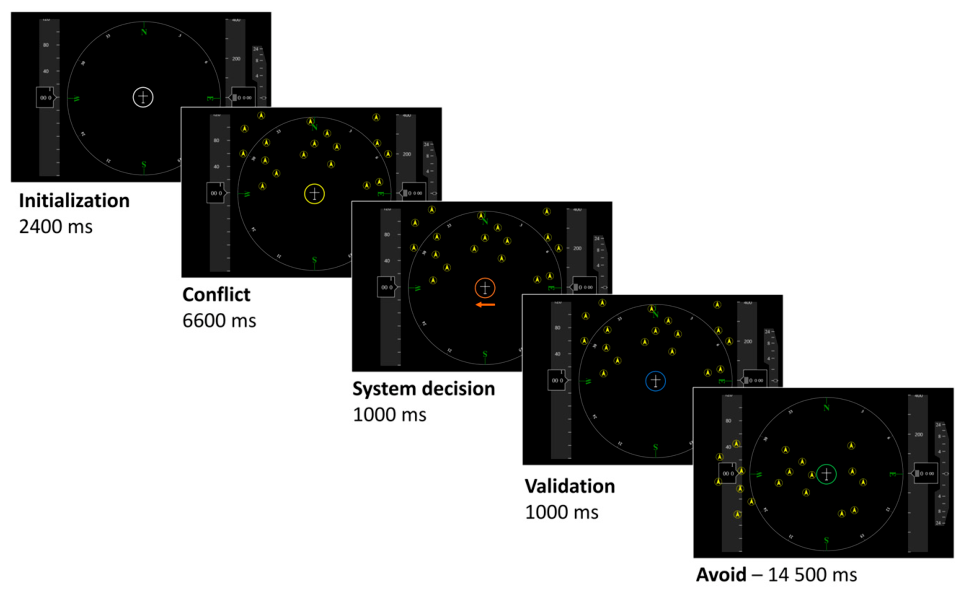
Figure 2.
Experimental saliency map for each HI state.
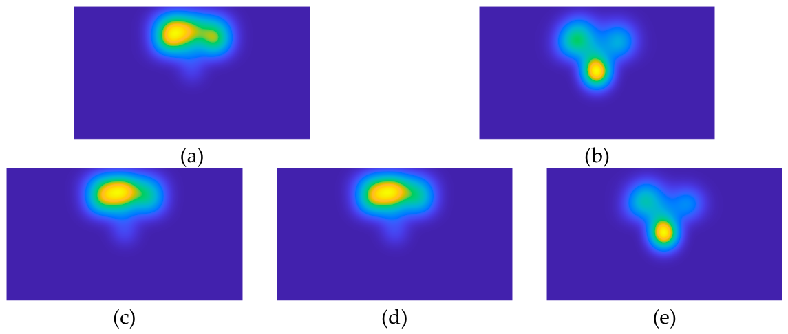
Figure 3.
Mean cumulative dwell time (± SE) obtained from the two-HI state SHMM showing (a) the main effect of HI state, (b) the main effect of ROI, and (c) the HI × ROI interaction. Bonferroni corrected p, * p < 0.05, ** p < 0.01, and *** p < 0.001.
Figure 3.
Mean cumulative dwell time (± SE) obtained from the two-HI state SHMM showing (a) the main effect of HI state, (b) the main effect of ROI, and (c) the HI × ROI interaction. Bonferroni corrected p, * p < 0.05, ** p < 0.01, and *** p < 0.001.
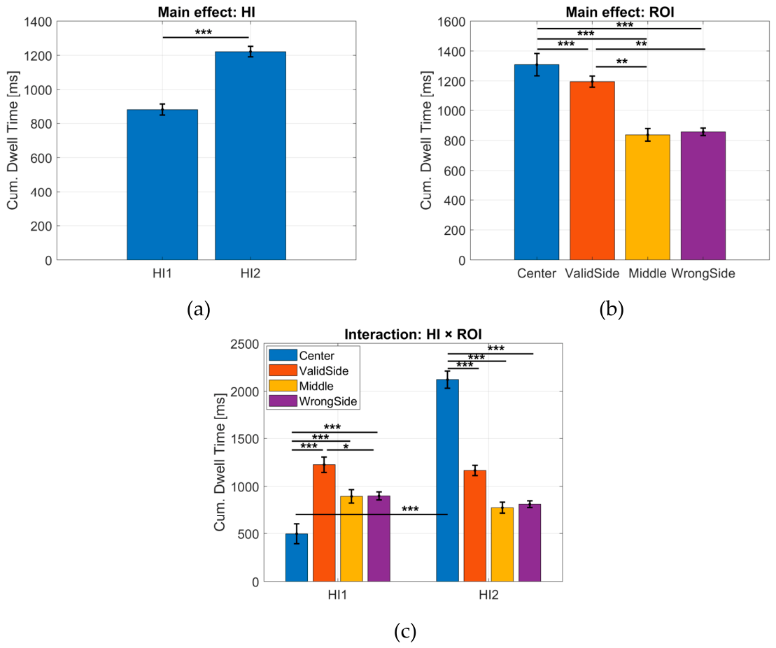
Figure 5.
Mean (± SE) of the absolute gap, measured as the difference between RT and transition time, as a function of transition type, based on individual means.
Figure 5.
Mean (± SE) of the absolute gap, measured as the difference between RT and transition time, as a function of transition type, based on individual means.
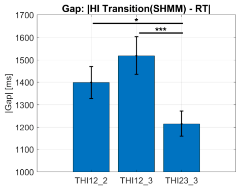
Figure 6.
Comparison of the fit quality of LMMs of increasing complexity based on (a) the Akaike Information Criterion (AIC) and (b) the adjusted coefficient of determination (R²).
Figure 6.
Comparison of the fit quality of LMMs of increasing complexity based on (a) the Akaike Information Criterion (AIC) and (b) the adjusted coefficient of determination (R²).
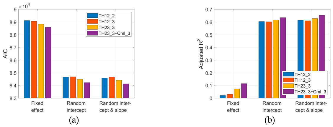

Table 1.
Summary of initialization and configuration parameters for SHMMs.
| Configuration\Initialization | S=2, R=4 | S=3, R=4 |
|---|---|---|
| Prior probabilities of HI states | ||
| HI state transition matrix | ||
| ROI transition matrix | Random | |
| Means and variances (ROIs), Gaussian density | From KMeans (K=R) | |
| Stopping criteria | Log-Likelihood decrease < 1.10⁻⁵ ; max 10,000 iterations | |
Table 2.
Post-hoc comparisons of KL divergences between the HI states (mean ± SE, F(1,260) statistics, and corrected p-values). Significant differences are indicated in bold.
Table 2.
Post-hoc comparisons of KL divergences between the HI states (mean ± SE, F(1,260) statistics, and corrected p-values). Significant differences are indicated in bold.
| Group 1: Final states | Group 2: Early states | ||||
|---|---|---|---|---|---|
|
Moy ±SE |
HI2_2 | HI3_3 | HI1_2 | HI1_2 | HI2_3 |
| 0.14 ± 0.03 | 0.17 ± 0.02 | 0.32 ± 0.03 | 0.39 ± 0.03 | 0.55 ± 0.04 | |
| HI2_2 | - | 1.18, p=1.00 | 15.76, p<0.0001 | 23.36, p<0.0001 | 29.89, p<0.0001 |
| HI3_2 | - | - | 8.32, p<0.05 | 14.05, p<0.01 | 19.21, p<0.001 |
| HI1_2 | - | 0.74, p=1.00 | 2.24, p=1.00 | ||
| HI1_2 | - | - | - | - | 0.40, p=1.00 |
| HI2_3 | - | - | - | - | - |
Table 3.
Descriptive statistics of the gap distributions between the adjacent HI state transition times and reaction times (RT), for the three distinct transition time estimates.
Table 3.
Descriptive statistics of the gap distributions between the adjacent HI state transition times and reaction times (RT), for the three distinct transition time estimates.
| Transition | Average [ms] | Std [ms] | Skewness | Kurtosis |
|---|---|---|---|---|
| THI12_2 | -38.99 | 1,711.88 | -0.21 | 2.99 |
| THI12_3 | -1,104.06 | 1,442.99 | 0.04 | 3.25 |
| THI23_3 | 392.30 | 1,463.19 | -0.16 | 3.30 |
Table 4.
Fit and quality parameters (adjusted coefficient of determination, residual standard deviation, AIC, and log-likelihood) of the LMMs that explain reaction time (RT) by transition time (THI12_2, THI12_3, or THI23_3). For the best fit obtained with THI23_3 as the explanatory variable (in bold in the table), the log-likelihood of state restoration by the SHMM for each trial (Cml_3) was added as an additional explanatory variable.
Table 4.
Fit and quality parameters (adjusted coefficient of determination, residual standard deviation, AIC, and log-likelihood) of the LMMs that explain reaction time (RT) by transition time (THI12_2, THI12_3, or THI23_3). For the best fit obtained with THI23_3 as the explanatory variable (in bold in the table), the log-likelihood of state restoration by the SHMM for each trial (Cml_3) was added as an additional explanatory variable.
| Transi- tion |
Parameters | Fixed effect | Random effect: Intercept | Random effect: Intercept & slope |
|---|---|---|---|---|
| THI12_2 | 0 ± SE [ms] | 2713.1 ± 38.491 | 2868.5 ± 133.44 | 2851.1 ± 144.55 |
| 1 ± SE | 0.1221 ± 0.0115 | 0.0912 ± 0.0080 | 0.0947 ± 0.0152 | |
| Adjusted R2 | 0.0212 | 0.6044 | 0.6153 | |
| Residual std | 1176.1 | 748.39 | 738.66 | |
| AIC | 89122 | 84646 | 84575 | |
| Log likelihood | -44558 | -42319 | -42282 | |
| THI12_3 | 0 ± SE [ms] | 2692 ± 34.412 | 2926.6 ± 131.89 | 2920.5 ± 169.51 |
| 1 ± SE | 0.1984 ± 0.0153 | 0.1106 ± 0.0110 | 0.1178 ± 0.0194 | |
| Adjusted R2 | 0.0307 | 0.6022 | 0.6102 | |
| Residual std | 1170.2 | 750.43 | 743.14 | |
| AIC | 89070 | 84673 | 84648 | |
| Log likelihood | -44532 | -42333 | -42318 | |
| THI23_3 | 0 ± SE [ms] | 2182.3 ± 47.388 | 2567.9 ± 131.75 | 2531 ± 144.58 |
| 1 ± SE | 0.2596 ± 0.0128 | 0.1659 ± 0.0096 | 0.1699 ± 0.0183 | |
| Adjusted R2 | 0.0720 | 0.6166 | 0.6281 | |
| Residual std | 1145 | 736.89 | 726.35 | |
| AIC | 88841 | 84482 | 84408 | |
| Log likelihood | -44418 | -42237 | -42198 | |
| THI23_3 + Cml_3 | 0 ± SE [ms] | 1362.8 ± 69.67 | 1924 ± 135.26 | 1912.7 ± 196.37 |
| 1 ± SE | 0.2311 ± 0.0127 | 0.1454 ± 0.0094 | 0.1447 ± 0.0175 | |
| 2 ± SE | -9.7703 ± 0.6206 | -7.5870 ± 0.4616 | -7.7111 ± 0.8738 | |
| Adjusted R2 | 0.1137 | 0.6354 | 0.6532 | |
| Residual std | 1118.9 | 718.57 | 702.09 | |
| AIC | 88601 | 84221 | 84119 | |
| Log likelihood | -44297 | -42105 | -42050 |
Disclaimer/Publisher’s Note: The statements, opinions and data contained in all publications are solely those of the individual author(s) and contributor(s) and not of MDPI and/or the editor(s). MDPI and/or the editor(s) disclaim responsibility for any injury to people or property resulting from any ideas, methods, instructions or products referred to in the content. |
© 2026 by the authors. Licensee MDPI, Basel, Switzerland. This article is an open access article distributed under the terms and conditions of the Creative Commons Attribution (CC BY) license (http://creativecommons.org/licenses/by/4.0/).
Copyright: This open access article is published under a Creative Commons CC BY 4.0 license, which permit the free download, distribution, and reuse, provided that the author and preprint are cited in any reuse.