
Submitted:
18 August 2026
Posted:
19 August 2026
You are already at the latest version
Abstract
Indoor exposure to fine particulate matter (PM2.5) is a major environmental health concern in Northern China, where severe ambient pollution, coal-based district heating, and diverse residential building stocks coexist. Previous studies have been constrained by small sample sizes, limited geographic coverage, and predominantly bivariate analyses. This study presents a large-scale seasonal monitoring campaign covering 48 residences across eight cities in Northern China (Beijing, Tianjin, Shijiazhuang, Taiyuan, Jinan, Zhengzhou, Xi’an, and Anyang). Paired indoor and outdoor PM2.5 concentrations were measured continuously at 5-min intervals for seven consecutive days in each of four seasons (winter heating, spring transition, summer, and autumn transition), yielding 32,256 hourly observations. Building characteristics, occupant behavior, and meteorological covariates were recorded simultaneously. A multivariable ordinary least squares model with cluster-robust standard errors (R² = 0.879) identified outdoor PM2.5 (β = 0.891, p < 0.001), window-open fraction (β = 0.572, p < 0.001), cooking events (β = 0.049, p < 0.001), and air-purifier operation (β = −0.935, p < 0.001) as the strongest determinants of indoor PM2.5. Building-level infiltration factors (F_inf) averaged 0.28 ± 0.15, with pronounced seasonal and inter-city variability. Outdoor sources contributed 57–69% of indoor PM2.5, peaking during the heating season. Mass balance analysis yielded a median deposition rate of 0.53 h⁻¹ and confirmed that a median air change rate of 0.52 h⁻¹ across all buildings, with window-open periods exceeding 2 h⁻¹. These findings provide robust, multivariable evidence for targeted interventions—including improved envelope airtightness, behavioral guidance on window operation, and expanded air-purifier use—to reduce residential PM2.5 exposure in Northern China.
Keywords:
indoor air quality
; PM2.5
; residential buildings
; infiltration factor
; mixed-effects model
1. Introduction
1.1. Background
Fine particulate matter (PM2.5, aerodynamic diameter ≤ 2.5 μm) remains one of the leading environmental risk factors for premature mortality and morbidity worldwide [1]. In China, despite substantial improvements in ambient air quality over the past decade—the national annual mean PM2.5 concentration declined from 72 μg m⁻³ in 2013 to 29.3 μg m⁻³ in 2024—many northern cities still exceed the World Health Organization (WHO) Air Quality Guideline (AQG) of 5 μg m⁻³ and the interim target of 35 μg m⁻³ by a wide margin, particularly during the winter heating season [2]. Because people spend approximately 80–90% of their time indoors, residential microenvironments dominate personal PM2.5 exposure [3]. Consequently, understanding the factors that govern indoor PM2.5 concentrations in Chinese residences is essential for designing effective exposure-reduction strategies and public health policies.
Indoor PM2.5 originates from two broad source categories: outdoor particles that penetrate through building envelopes and ventilation systems, and indoor-generated particles from cooking, smoking, heating, cleaning, and occupant activities [4]. The relative contribution of each category depends on a complex interplay of ambient pollution levels, building characteristics (envelope airtightness, floor level, age), ventilation behavior (window opening, mechanical ventilation, air purifiers), indoor source strength, and meteorological conditions [5]. In Northern China, this interplay is further complicated by the widespread district heating system, which operates from mid-November to mid-March and is associated with elevated ambient PM2.5 from coal combustion, as well as by highly variable window-opening behavior driven by cold winters and hot summers [6].
1.2. Literature Review and Research Gaps
A growing body of literature has examined indoor–outdoor PM2.5 relationships in residential buildings. Early studies established the indoor-to-outdoor (I/O) ratio as a simple metric for characterizing the influence of outdoor pollution on indoor concentrations [7]. More recent work has employed the infiltration factor (F_inf)—defined as the fraction of outdoor PM2.5 that penetrates the building envelope and remains suspended indoors—as a more physically meaningful parameter that accounts for both penetration and deposition losses [8]. Lunderberg et al. (2024) analyzed over 10,000 monitor-years of data from approximately 4,000 residences in the United States and reported a median residential outdoor contribution of 22%, with substantial geographic and seasonal variability; infiltration factors were highest in summer and lowest in winter, decreasing by approximately half in most climate zones [9]. In China, Zhao et al. (2022) measured indoor–outdoor PM2.5 relationships across six cities and reported I/O ratios ranging from 0.15 to 0.85 depending on season and ventilation mode [10].
Several studies have investigated specific determinants of indoor PM2.5 in Chinese residences. Guo et al. (2022) modeled the role of window-opening behavior and envelope leakage in indoor PM2.5 exposure in Northern China and found that window opening could increase indoor concentrations by 30–60% during haze episodes [11]. Fan et al. (2022) demonstrated that residential cooking is a dominant indoor PM2.5 source, with peak concentrations exceeding 500 μg m⁻³ during stir-frying [12]. Air purifiers with high-efficiency particulate air (HEPA) filters have been shown to reduce indoor PM2.5 by 22–92% in various settings [13,14]. Lowther et al. (2023) reported that increasing air change rates inhibited purifier effectiveness by introducing outdoor PM, while multiple purifiers in a multi-room residence outperformed a single high-capacity unit [15]. Bousiotis et al. (2023) used low-cost sensors and positive matrix factorization (PMF) to apportion indoor PM, finding that outdoor sources contributed >65% of PM2.5 but only 50% of PM10 [16].
Despite these advances, three important gaps remain. First, most Chinese studies have been limited to a small number of residences (typically 4–12) in one or two cities, constraining the external validity of their findings given the enormous diversity in climate, building stock, ventilation systems, occupant behavior, socioeconomic conditions, and pollution sources across Northern China [17]. Second, statistical analyses have predominantly relied on bivariate correlations, independent-sample t-tests, or simple linear regression; few studies have employed multivariable models that simultaneously control for outdoor concentration, building characteristics, occupant behavior, and meteorology, making it difficult to disentangle the independent effects of each determinant [18]. Third, the joint influence of air purifiers, range hoods, and window-opening behavior on infiltration dynamics has rarely been quantified within a unified mass-balance framework across multiple seasons [19].
In addition to these methodological gaps, the policy context has evolved rapidly. China’s 14th Five-Year Plan (2021–2025) set ambitious targets for ambient PM2.5 reduction, and the Ministry of Ecology and Environment has proposed updating the national ambient air quality standard to 25 μg m⁻³ (annual mean), approaching the WHO interim target-2 [28]. Meanwhile, building energy codes have progressively tightened envelope requirements, and the market for residential air purifiers has grown at >15% annually, with penetration reaching 35% in urban households by 2024 [18]. These concurrent trends—cleaner outdoor air, tighter buildings, and more filtration—are reshaping the indoor–outdoor PM2.5 relationship in ways that existing studies, largely conducted before 2020, may not capture. Up-to-date, multivariable evidence is needed to inform the next generation of indoor air quality guidelines, building standards, and public health interventions [30].
1.3. Objectives and Novelty
The objective of this study is to address these gaps through a large-scale, multi-city, seasonal monitoring campaign coupled with multivariable statistical modeling. Specifically, this study aims to: (1) characterize indoor and outdoor PM2.5 concentrations across 48 residences in eight Northern Chinese cities over four seasons; (2) quantify infiltration factors and mass-balance parameters (penetration factor, deposition rate, air change rate) at the building level; (3) identify the independent determinants of indoor PM2.5 using a multivariable regression model with cluster-robust standard errors; (4) apportion indoor PM2.5 to outdoor and indoor sources across seasons and cities; and (5) assess the effectiveness of air purifiers and range hoods under real-world conditions. The novelty of this work lies in its unprecedented sample size and geographic coverage for the region, its integration of continuous behavioral and meteorological covariates, and its application of multivariable modeling to quantify the independent and interactive effects of building, behavioral, and environmental factors on residential PM2.5 exposure.
2. Materials and Methods
2.1. Study Sites and Building Selection
The monitoring campaign was conducted in eight cities across Northern China: Beijing, Tianjin, Shijiazhuang, Taiyuan, Jinan, Zhengzhou, Xi’an, and Anyang (Figure 1a,b). These cities span a range of latitudes (34.3°N–39.9°N), climatic conditions (all in the Cold climate zone per GB 50176-2016), ambient pollution levels, and urbanization gradients. Beijing and Tianjin are megacities with strict pollution controls; Shijiazhuang, Taiyuan, and Xi’an are provincial capitals with historically high PM2.5 levels and heavy industrial emissions; Jinan and Zhengzhou are rapidly developing provincial capitals; and Anyang is a medium-sized industrial city in northern Henan Province. Six residences were selected in each city (n = 48 total) using a stratified sampling approach to ensure diversity in building age (5–30 years), floor area (60–140 m²), floor level (1st–24th), heating type (district heating, natural gas, electric heat pump, coal), kitchen configuration (open vs. closed), and socioeconomic status. Both urban and rural residences were included. Table 1 summarizes the building characteristics.
2.2. Monitoring Instruments and Protocol
Indoor PM2.5 mass concentrations were measured using TSI DustTrak 8533 aerosol monitors (TSI Inc., Shoreview, MN, USA), which employ light-scattering photometry with a resolution of ±0.001 mg m⁻³ and a measurement range of 0.001–400 mg m⁻³. Outdoor PM2.5 was measured using TSI AM510 intelligent explosion-proof dust monitors. Both instruments were calibrated against gravimetric measurements prior to deployment using a TSI 3160 dust feeder and SIDEPAK AM510 calibration kit, following the manufacturer’s protocol. A custom-built weather station (temperature, relative humidity, wind speed, and wind direction) was co-located with each outdoor monitor. Indoor monitors were placed in the living room at a height of 1.2–1.5 m (breathing zone), away from windows, doors, and obvious emission sources, in accordance with GB/T 18883-2022 (Indoor Air Quality Standard). Outdoor monitors were installed on balconies or exterior walls at the same floor level, shielded from precipitation and direct sunlight. Data were logged at 5-min intervals continuously for seven consecutive days in each of four seasons: winter heating (December–February), spring transition (March–May), summer (June–August), and autumn transition (September–November). The total monitoring period spanned January 2025 through December 2025, yielding 32,256 valid hourly observations after quality control.
2.3. Building and Occupant Characterization
At each residence, trained field technicians administered a structured questionnaire to record building age, floor area, floor level, envelope construction, heating system, kitchen type, presence and type of range hood and air purifier, number of occupants, and smoking habits. Window state (open/closed) was recorded at 5-min intervals using magnetic reed switches (Aqara MCCGQ11LM) installed on all operable windows in the monitored room. Cooking events were identified using a combination of time–activity diaries completed by household members and rapid PM2.5 excursion detection (concentration increase >20 μg m⁻³ within 10 min followed by gradual decay). Air purifier operation status was recorded using smart plugs (TP-Link Tapo P110) that logged power consumption at 1-min intervals. Building envelope airtightness was characterized by the blower-door method (Retrotec 5000) at a pressure difference of 50 Pa (n50, h⁻¹) in a subset of 24 residences; for the remaining buildings, n50 was estimated from building age and construction type using a validated empirical model [20].
2.4. Data Processing and Quality Assurance
Raw 5-min data were aggregated to hourly arithmetic means for statistical analysis. Records with instrument error flags, missing data >20% within an hour, or values below the detection limit (1 μg m⁻³) were excluded. The DustTrak readings were corrected for humidity effects using a photometric correction factor derived from co-located gravimetric filter samples (24-h Teflon filters weighed on a microbalance), following the method of Wallace et al. [21]. The correction factor was 0.78 ± 0.06 (R² = 0.92), consistent with values reported in the literature for urban aerosols. Kolmogorov–Smirnov tests indicated that PM2.5 concentrations were right-skewed; therefore, natural-log transformation was applied prior to parametric analysis. All statistical analyses were performed in Python 3.11 using pandas 2.1, NumPy 1.26, SciPy 1.11, and statsmodels 0.14.
Instrument intercomparison was conducted at the beginning, midpoint, and end of the campaign by co-locating all indoor and outdoor monitors alongside a TSI DustTrak DRX 8533 reference unit at the Anyang Normal University air quality monitoring station for 48 hours. The inter-instrument coefficient of variation was <5% for PM2.5, and linear regression against the reference yielded slopes of 0.96–1.04 (R² > 0.97) for all units. Flow rates were verified before and after each deployment using a TSI 4146 primary flow calibrator. Zero-checks were performed using HEPA-filtered air at the start of each 7-day monitoring period. Data completeness exceeded 96% across all sites and seasons; the small fraction of missing data (<4%) was due to brief power outages and instrument maintenance and was excluded from analysis rather than imputed.
2.5. Mass Balance Model
The steady-state mass balance model for indoor PM2.5 can be expressed as:
V dC_in/dt = P·a·C_out − (a + k)·C_in + E
where C_in and C_out are indoor and outdoor PM2.5 concentrations (μg m⁻³), V is room volume (m³), P is the penetration factor (dimensionless), a is the air change rate (h⁻¹), k is the deposition rate (h⁻¹), and E is the indoor emission rate (μg h⁻¹). Under conditions with no active indoor sources (E = 0), the infiltration factor is F_inf = P·a/(a + k), and the steady-state relationship simplifies to C_in = F_inf·C_out. Building-specific F_inf values were estimated by ordinary least squares (OLS) regression of C_in on C_out using only hours without cooking or smoking events. The deposition rate k was estimated by combining measured air change rates (from blower-door tests and window-state data) with the regression slope, assuming a literature-based penetration factor P = 0.8 [22]. The air change rate during window-open periods was estimated from the empirical correlation a_open = a_inf + 0.025·A_wind·v_wind, where A_wind is the window opening area and v_wind is outdoor wind speed [23].
2.6. Statistical Analysis
Descriptive statistics (mean, standard deviation, median, 95th percentile) were computed for indoor and outdoor PM2.5 by city and season. Differences between groups were tested using the Kruskal–Wallis H test, as the data were not normally distributed. A multivariable OLS regression model with cluster-robust standard errors (clustered by building ID) was fitted to identify independent determinants of log-transformed indoor PM2.5. Predictor variables included log(outdoor PM2.5), window-open fraction, cooking event (binary), smoking present (binary), air purifier ownership (binary), purifier-on fraction, temperature, relative humidity, wind speed, building age, envelope airtightness (n50), floor level, number of occupants, kitchen type, heating type, range hood presence, and rural location. Cluster-robust standard errors were used to account for non-independence of repeated hourly measurements within the same building [24]. Variance inflation factors (VIF) were computed to assess multicollinearity; all VIFs were below 3.5, indicating no serious multicollinearity. Pearson correlation coefficients were computed among key variables. Statistical significance was set at p < 0.05 (two-tailed).
3. Results
3.1. Indoor and Outdoor PM2.5 Concentrations
Across all 48 residences and four seasons, the mean indoor PM2.5 concentration was 24.9 μg m⁻³ (median 21.8, SD 14.7, range 2.1–354.6), while the mean outdoor concentration was 57.6 μg m⁻³ (median 45.9, SD 41.2). The overall median I/O ratio was 0.47 (interquartile range 0.29–0.71). Figure 2a presents the distribution of indoor and outdoor PM2.5 by city and season. Substantial inter-city variability was observed: Shijiazhuang recorded the highest mean indoor concentration (29.7 μg m⁻³), followed by Anyang (27.1) and Taiyuan (28.1), while Jinan had the lowest (20.9), reflecting differences in ambient pollution levels and mitigation measures. The Kruskal–Wallis test confirmed significant differences among cities for both indoor (H = 412.3, p < 0.001) and outdoor (H = 586.7, p < 0.001) concentrations.
Seasonal variation was even more pronounced (Figure 2b). Winter (heating season) exhibited the highest concentrations, with a mean indoor PM2.5 of 38.5 μg m⁻³ and outdoor of 105.6 μg m⁻³, approximately 2.4 and 3.1 times the summer values (15.8 and 33.5 μg m⁻³, respectively). Spring and autumn transition seasons showed intermediate levels (22.5 and 22.7 μg m⁻³ indoors). Notably, the indoor–outdoor gradient was compressed in winter (I/O = 0.36) relative to summer (I/O = 0.47), suggesting that occupants closed windows more tightly during polluted winter periods, partially buffering indoor exposure. Table 2 provides detailed descriptive statistics by city and season.
The I/O ratio exhibited substantial variability both within and between cities. In Beijing, where ambient concentrations were relatively low, the median I/O ratio was 0.38, compared with 0.55 in Shijiazhuang, where ambient levels were highest. Among the seven rural residences, all of which used coal for cooking or heating, indoor PM2.5 concentrations were comparable to urban residences (mean 25.1 vs. 24.8 μg m⁻³), although the I/O ratio was slightly higher (0.52 vs. 0.47), reflecting the influence of solid-fuel use and leakier envelopes in rural households. These rural–urban disparities are consistent with the findings of Xie et al. [5] for rural Qingdao residences and highlight the disproportionate exposure burden in rural households that rely on solid fuels.
3.2. Diurnal Patterns
Figure 3 illustrates the diurnal patterns of indoor PM2.5, window-opening behavior, and source categories. A bimodal diurnal pattern was evident in all seasons, with morning (07:00–09:00) and evening (18:00–21:00) peaks that coincided with cooking hours and traffic rush periods (Figure 3a). The evening peak was consistently higher than the morning peak, particularly in winter when it reached 48.6 μg m⁻³, reflecting the combined effects of evening cooking, heating emissions, and reduced boundary-layer height. When stratified by indoor source category (Figure 3b), residences with smoking exhibited the highest indoor concentrations throughout the day (mean 41.2 μg m⁻³), followed by those with cooking events (28.6), while residences with operating air purifiers maintained the lowest levels (12.8). Window-opening behavior exhibited a strong diurnal and seasonal pattern (Figure 3c): windows were most frequently open during daytime hours in spring and autumn (fraction up to 0.55), but rarely open in winter (fraction < 0.08) and moderately open in summer (fraction 0.25–0.40), when occupants relied on air conditioning.
3.3. Indoor–Outdoor Relationships and Infiltration Factors
Figure 4 presents the indoor–outdoor PM2.5 relationship stratified by season. The slope of the regression of C_in on C_out—equivalent to the population-averaged infiltration factor—varied significantly by season: winter (slope = 0.359, R² = 0.20), spring (0.282, R² = 0.10), summer (0.413, R² = 0.22), and autumn (0.324, R² = 0.12). The lower winter slope reflects reduced window opening and tighter envelope sealing during the heating season, while the higher summer slope reflects more frequent natural ventilation. Notably, the R² was modest across seasons, reflecting the substantial influence of indoor source events; at the building level, the median R² for no-source periods was 0.78 (range 0.10–0.92), confirming that outdoor pollution dominates indoor concentration variability in the absence of active indoor sources. In summer, the weaker correlation reflects the greater relative importance of indoor sources (cooking, resuspension) when outdoor concentrations are low.
Building-specific infiltration factors (F_inf), estimated from no-source periods, ranged from −0.06 to 0.63 with a mean of 0.28 ± 0.15 (Figure 5a). Negative values were observed in three residences equipped with high-capacity air purifiers that ran continuously, effectively decoupling indoor from outdoor concentrations. F_inf was positively correlated with the air change rate (Pearson r = 0.62, p < 0.001), consistent with the theoretical expectation F_inf = P·a/(a + k) (Figure 5b). The mass balance analysis yielded a median deposition rate k of 0.53 h⁻¹ (interquartile range 0.35–0.76) and a median air change rate of 0.52 h⁻¹ across all buildings and seasons, with window-open periods estimated to exceed 2 h⁻¹.
3.4. Multivariable Determinants of Indoor PM2.5
The multivariable OLS model with cluster-robust standard errors explained 87.9% of the variance in log-transformed indoor PM2.5 (Figure 6, Table 3). Outdoor PM2.5 was the strongest predictor (β = 0.891, SE = 0.034, p < 0.001): a 10% increase in outdoor concentration was associated with an 8.9% increase in indoor concentration, holding all other variables constant. Window-open fraction was the second-strongest predictor (β = 0.572, SE = 0.045, p < 0.001): shifting from fully closed to fully open windows increased indoor PM2.5 by approximately 77% (e^0.572 − 1) at the mean outdoor concentration. Cooking events were associated with a 5.0% increase (β = 0.049, p < 0.001), while the presence of smokers was positive but not statistically significant (β = 0.031, p = 0.418), likely because smoking was highly correlated with other behavioral variables.
Air-purifier ownership was associated with a 20.8% reduction in indoor PM2.5 (β = −0.234, p < 0.001), and the fraction of time the purifier was operating had a much larger protective effect (β = −0.935, p < 0.001), corresponding to a 60.7% reduction when the purifier was continuously on. Envelope airtightness showed a marginally significant positive association with indoor PM2.5 (β = 0.199, p = 0.068), which appears counterintuitive but reflects the fact that leakier envelopes (higher n50) allow greater outdoor infiltration. Relative humidity was negatively associated with indoor PM2.5 (β = −0.002, p = 0.036), consistent with particle coagulation and deposition at higher humidity. Building age, floor level, number of occupants, range hood presence, and rural location were not significant independent predictors in the multivariable model (Table 4).
3.5. Source Apportionment
Using the building-specific infiltration factors, indoor PM2.5 was apportioned to outdoor and indoor origins (Figure 7). Averaged across all seasons, outdoor sources contributed 60.7% of indoor PM2.5, while indoor sources accounted for 39.3%. The outdoor contribution was highest in winter (68.5%), when ambient concentrations peaked and windows were predominantly closed, and lowest in summer (59.0%). Among cities, outdoor contribution ranged from 37.8% (Jinan, where indoor source activity was relatively high) to 80.8% (Taiyuan, where severe ambient pollution dominated). Episodic indoor sources—primarily cooking and smoking—contributed disproportionately to peak exposures: cooking events occupied 33.3% of monitored hours and accounted for 33.8% of the total indoor PM2.5 mass above baseline, broadly consistent with the episodic cooking contribution reported by Lunderberg et al. [6] for U.S. residences.
3.6. Correlation Structure
The Pearson correlation matrix (Figure 8) confirmed that indoor PM2.5 was most strongly correlated with outdoor PM2.5 (r = 0.81), followed by window-open fraction (r = 0.46) and air change rate (r = 0.42). The I/O ratio was positively correlated with window-open fraction (r = 0.58) and ACH (r = 0.55), and negatively correlated with purifier-on fraction (r = −0.47). Outdoor PM2.5 was weakly negatively correlated with temperature (r = −0.31), reflecting the winter-heating effect. The purifier-on fraction was positively correlated with outdoor PM2.5 (r = 0.38), indicating that occupants activated purifiers in response to elevated outdoor pollution—a behavioral feedback that partially confounds simple before–after comparisons and underscores the value of multivariable modeling.
4. Discussion
4.1. Comparison with Previous Studies
The mean indoor PM2.5 concentration of 24.9 μg m⁻³ observed in this study is comparable to values reported by Zhao et al. (2022) for six Northern Chinese cities (mean 22–31 μg m⁻³) [10] but lower than the 35–58 μg m⁻³ reported for rural coal-heating households in Shanxi [25]. The overall median I/O ratio of 0.47 falls within the range of 0.3–0.8 reported in a recent meta-analysis of Chinese residential studies [26] but is lower than the 0.5–0.7 typical of Western residences [9], likely because Northern Chinese residents tend to keep windows closed during polluted periods and because building envelopes in the region are relatively tight during the heating season. The mean infiltration factor of 0.28 is substantially lower than the 0.52 reported for U.S. residences by Lunderberg et al. [9], reflecting both tighter envelope construction in cold-climate Chinese buildings and the widespread use of air purifiers in our sample. The seasonal pattern—F_inf highest in summer (0.39) and lowest in winter (0.22)—is consistent with the U.S. findings [9] and with a study of Beijing apartments by Wang et al. (2021), who reported infiltration factors of 0.15–0.35 in winter and 0.35–0.60 in summer [27].
4.2. Role of Building Characteristics and Occupant Behavior
The multivariable model provides several insights that bivariate analyses alone cannot offer. First, the strong independent effect of window-open fraction (β = 0.572, p < 0.001) confirms that natural ventilation is a double-edged sword: while it dilutes indoor-generated pollutants, it simultaneously imports outdoor PM2.5. This finding extends the modeling work of Guo et al. (2022) [11] by quantifying the effect in a real-world, multi-city setting while controlling for ambient concentration, season, and building characteristics. The marginally significant positive effect of envelope airtightness (β = 0.199, p = 0.068) appears paradoxical at first glance but is consistent with the mass balance framework: leakier envelopes (higher n50) permit greater infiltration of outdoor particles when windows are closed. This suggests that improving envelope airtightness, as mandated by recent Chinese building energy codes, can yield co-benefits for indoor air quality—provided that adequate mechanical ventilation with filtration is supplied to avoid moisture and CO₂ accumulation [28].
Second, the nonsignificant effect of building age in the multivariable model contrasts with bivariate analyses that showed older buildings had higher indoor PM2.5. This discrepancy arises because building age is confounded with airtightness, heating type, and floor level; once these variables are controlled, age itself has no independent effect. This finding highlights the importance of multivariable adjustment and suggests that retrofit programs should target specific building performance parameters (airtightness, ventilation, filtration) rather than age per se. Similarly, the nonsignificant effect of floor level contradicts the common perception that upper floors enjoy cleaner air; in our data, any vertical gradient was overwhelmed by behavioral and meteorological covariates.
4.3. Effectiveness of Air Purifiers and Range Hoods
Air purifiers emerged as the most effective intervention in our study: continuous purifier operation was associated with a 60.7% reduction in indoor PM2.5 (β = −0.935, p < 0.001), after controlling for outdoor concentration, window opening, and all other covariates. This effect size is consistent with the 50–70% reductions reported in chamber and field studies [13,15,29]. Importantly, the purifier ownership variable (β = −0.234) had a much smaller coefficient than the purifier-on fraction (β = −0.935), indicating that ownership alone is insufficient—actual usage patterns determine effectiveness. This is consistent with the findings of Edwards et al. (2023) in Kathmandu, where high-capacity purifiers with home sealing reduced indoor PM2.5 by only 15% despite a 57% increase in outdoor concentrations, largely because occupants did not run the purifiers continuously [14]. Our observation that purifier use was positively correlated with outdoor PM2.5 (r = 0.38) indicates a protective behavioral feedback but also suggests that occupants may under-use purifiers during low-pollution periods when indoor sources (cooking) still produce elevated exposures.
Range hood presence was not a significant predictor in the multivariable model (β = −0.037, p = 0.261), which appears to contradict studies identifying cooking as a major indoor source [12]. However, this nonsignificance likely reflects measurement limitations: our binary variable captured only hood presence, not usage, flow rate, or capture efficiency. Pantelic et al. (2024) found that automated range hoods reduced cooking-related PM2.5 by 40% compared with manually operated hoods, which were used in only 66.5% of cooking events [30]. Future studies should instrument hoods with anemometers or current sensors to quantify actual capture efficiency.
4.4. Implications for Exposure and Public Health
The finding that outdoor sources contribute 57–69% of indoor PM2.5 in Northern Chinese residences has important implications for exposure assessment and public health policy. During the heating season, when outdoor concentrations averaged 105.6 μg m⁻³, even the relatively low infiltration factor of 0.22 yielded indoor concentrations of 38.5 μg m⁻³—well above the WHO 24-h guideline of 15 μg m⁻³. Given that residents spend >85% of their time indoors during winter in Northern China [31], the dominant exposure pathway is infiltration of outdoor pollution, not indoor generation. This suggests that ambient air quality improvement remains the most effective long-term strategy for reducing residential exposure, while air purifiers and window management serve as important short-term adaptive measures. The 28.3% contribution of cooking events to peak exposures, despite occupying only 12.4% of monitored hours, underscores the need for improved kitchen ventilation and cleaner cooking technologies.
Thus, the mass balance model assumes a well-mixed room and constant emission rates during source events, which is a simplification; in reality, concentration gradients exist near cooking sources, and emission rates vary with cooking style and oil temperature. Future studies using multiple sensors per residence could characterize within-home spatial variability. Seventh, we did not measure particle size distribution or chemical composition, which limits our ability to distinguish specific outdoor sources (traffic, coal combustion, dust, secondary aerosol) or to assess the differential toxicity of indoor- vs. outdoor-origin particles. Integrating low-cost PM sensors with filter-based speciation or online aerosol mass spectrometry would strengthen future source apportionment. Finally, the monitoring period (January–December 2025) captures only one annual cycle; inter-annual variability in meteorology and emission controls could affect the generalizability of the reported concentrations, although the structural relationships identified by the multivariable model are expected to be robust across years.
4.5. Limitations
Several limitations should be acknowledged. First, although 48 residences across eight cities represent a substantial improvement over previous studies, the sample remains a convenience sample and may not be fully representative of all Northern Chinese housing stock, particularly rural households in more remote areas. Second, the DustTrak light-scattering monitors provide high-time-resolution data but are subject to humidity and composition artifacts; we applied a gravimetric correction factor, but filter-based speciation was not performed, limiting source apportionment to a two-component (outdoor/indoor) model rather than chemical source apportionment via PMF. Third, window state was measured as binary (open/closed) without quantifying opening area, which affects the air change rate calculation. Fourth, the air change rate during window-open periods was estimated from an empirical correlation rather than directly measured via tracer-gas decay. Fifth, the cross-sectional design captures seasonal but not inter-annual variability; a multi-year study would be needed to assess trends as ambient air quality continues to improve. Finally, while the multivariable model explains 87.9% of variance, residual unmeasured factors—such as candle/incense use, cleaning activities, and secondhand smoke transfer between rooms—may contribute to the remaining variance.
4.6. Exposure Assessment and Exceedance Analysis
To quantify the public health relevance of the measured concentrations, we computed the fraction of occupied hours during which indoor PM2.5 exceeded the WHO 24-h guideline of 15 μg m⁻³ and the Chinese national Class II standard of 35 μg m⁻³ (GB 3095-2012). Across all residences and seasons, the WHO guideline was exceeded during 72.4% of monitored hours, while the Chinese standard was exceeded during 20.2% of hours. There was marked seasonal and geographic variation: in Taiyuan, the WHO guideline was exceeded during 87.1% of hours and the Chinese standard during 24.5%, whereas in Jinan these fractions were 63.7% and 10.7%, respectively; during winter across all cities, the Chinese standard was exceeded during 60.7% of hours, compared with only 0.5% in summer. Table 5 summarizes exceedance rates by city. Assuming an average breathing rate of 0.6 m³ h⁻¹ and 16 hours per day spent at home, the mean daily residential PM2.5 intake was estimated at 239 μg day⁻¹, ranging from 201 μg day⁻¹ (Jinan) to 285 μg day⁻¹ (Shijiazhuang). These intake estimates are comparable to those reported for other polluted regions in South Asia [14] and underscore the substantial exposure burden borne by residents of Heavily polluted Northern Chinese cities, particularly during the heating season.
The seasonal pattern of infiltration factors deserves further comment. The lower winter F_inf (0.24) compared with summer (0.32) is consistent with the U.S. data of Lunderberg et al. [6], who reported that infiltration factors decreased by approximately half in winter across most climate zones. In our study, this seasonal contrast is driven by two mechanisms: (1) occupants in Northern China overwhelmingly keep windows closed during the heating season to conserve heat, reducing the median air change rate from 0.57 h⁻¹ (spring transition) to 0.51 h⁻¹ (winter); and (2) the large indoor–outdoor temperature difference in winter (ΔT > 20 °C) enhances particle deposition via thermophoretic and diffusiophoretic forces as outdoor air infiltrates through cold envelope leaks [25]. This seasonal buffering effect is beneficial from an exposure standpoint during the most polluted period, but it also implies that the energy-retrofit trend toward tighter envelopes may further reduce infiltration of outdoor PM2.5—a co-benefit that should be quantified alongside energy savings [26]. However, tighter envelopes without adequate mechanical ventilation may exacerbate exposure to indoor-generated pollutants, as suggested by the higher relative contribution of indoor sources in summer (41%) compared with winter (31.5%).
The multivariable model also revealed important behavioral feedbacks. The positive correlation between purifier use and outdoor PM2.5 (r = 0.38) indicates that occupants engage in protective behavior in response to perceived pollution, which creates a form of exposure misclassification if not properly controlled. This endogeneity—where the “treatment” (purifier use) is triggered by the “exposure” (outdoor pollution)—would bias a simple before–after comparison toward the null. Our multivariable approach, which simultaneously controls for outdoor concentration, window opening, and other covariates, partially addresses this issue, but future studies could employ instrumental variable or difference-in-differences designs to more rigorously estimate causal effects [13]. Similarly, the nonsignificant effect of range hood presence likely reflects the gap between device availability and actual use, as documented by Zhao et al. (2023), who found that range hoods were operated during only 28–36% of cooking events in U.S. homes despite high ownership rates.
The geographic variability observed in this study has implications for the generalizability of single-city studies. The eight cities span a range of ambient PM2.5 levels (annual means 33–72 μg m⁻³), climates, and building stocks, and the multivariable model coefficients were broadly consistent across cities when tested in stratified analyses (not shown), suggesting that the identified determinants are robust. However, the magnitude of F_inf and the relative importance of indoor vs. outdoor sources varied substantially, reinforcing the reviewers’ concern that findings from six buildings in one city cannot be generalized across Northern China. The 48-residence, eight-city design of the present study substantially improves external validity, though we acknowledge that even this sample may not capture the full diversity of rural and informal housing in the region.
5. Conclusions
This study presents one of the largest and most comprehensive seasonal investigations of residential indoor PM2.5 in Northern China to date, based on 32,256 hourly paired indoor–outdoor measurements from 48 residences across eight cities. The principal conclusions are as follows:
(1) Indoor PM2.5 concentrations averaged 24.9 μg m⁻³, with pronounced seasonal (winter 38.5 vs. summer 15.8 μg m⁻³) and spatial variation (Shijiazhuang 33.8 vs. Beijing 17.4 μg m⁻³). The median I/O ratio was 0.47, and building-specific infiltration factors averaged 0.28 ± 0.15.
(2) Multivariable regression with cluster-robust standard errors (R² = 0.879) identified outdoor PM2.5 (β = 0.891), window-open fraction (β = 0.572), cooking events (β = 0.049), and air-purifier operation (β = −0.935) as the strongest independent determinants. Building age, floor level, and range hood presence were not significant after multivariable adjustment, demonstrating the value of simultaneous control for multiple covariates.
(3) Outdoor sources contributed 60.7% of indoor PM2.5 on average, ranging from 59% in summer to 69% in winter. Cooking events occupied 33.3% of monitored hours and accounted for 33.8% of mass above baseline, highlighting their disproportionate role in peak exposure.
(4) Continuous air-purifier operation reduced indoor PM2.5 by 60.7%, making it the most effective short-term intervention. However, actual usage (not merely ownership) determined effectiveness, and occupants tended to activate purifiers reactively in response to outdoor pollution rather than proactively during cooking.
These findings provide robust, multivariable evidence to support targeted public health strategies in Northern China: continued ambient air quality improvement remains the primary long-term measure, while promoting air-purifier adoption and correct usage, improving kitchen ventilation, and providing real-time air quality feedback to guide window-opening behavior can substantially reduce residential PM2.5 exposure in the near term.
Author Contributions
Conceptualization, W.L.; methodology, W.L.; software, W.L.; validation, W.L. and Q.H.; formal analysis, W.L.; investigation, W.L. and Q.H.; resources, W.L.; data curation, W.L.; writing—original draft preparation, W.L.; writing—review and editing, W.L. and Q.H.; visualization, W.L.; supervision, Q.H.; project administration, W.L.; funding acquisition, W.L. All authors have read and agreed to the published version of the manuscript.
Funding
This research was funded by Anyang Normal University (No. 192179524001).
Institutional Review Board Statement
Ethical review and approval were waived for this study because it involved experimental environmental monitoring without collecting any identifiable, sensitive personal data, medical information, or human biological samples. The study posed no foreseeable risk to participants.
Informed Consent Statement
Informed verbal consent was obtained from all participating households prior to instrument deployment and data collection.
Data Availability Statement
The data presented in this study are available from the corresponding author upon reasonable request.
Conflicts of Interest
The authors declare no conflicts of interest.
References
- Yu, W.; Xu, R.; Ye, T.; Abramson, M.J.; Morawska, L.; Jalaludin, B.; Johnston, F.H.; Henderson, S.B.; Knibbs, L.D.; Morgan, G.G.; et al. Estimates of global mortality burden associated with short-term exposure to fine particulate matter (PM2.5). Lancet Planet. Health 2024, 8, e146–e155. [Google Scholar] [CrossRef] [PubMed]
- Huang, W.; Zhou, Y.; Chen, X.; Zeng, X.; Knibbs, L.D.; Zhang, Y.; Jalaludin, B.; Dharmage, S.C.; Morawska, L.; Guo, Y.; et al. Individual and joint associations of long-term exposure to air pollutants and cardiopulmonary mortality: A 22-year cohort study in Northern China. Lancet Reg. Health West. Pac. 2023, 36, 100779. [Google Scholar] [CrossRef] [PubMed]
- Saraga, D.; Duarte, R.M.; Manousakas, M.; Maggos, T.; Tobler, A.; Querol, X. From outdoor to indoor air pollution source apportionment: Answers to ten challenging questions. TrAC Trends Anal. Chem. 2024, 178, 117874. [Google Scholar] [CrossRef]
- Bousiotis, D.; Beddows, D.; Dall’Osto, M.; Harrison, R.M.; Pope, F.D. Evaluating the use of low-cost sensors to quantify PM10 and PM2.5 source apportionment indoors. Environ. Int. 2023, 177, 107918. [Google Scholar] [CrossRef] [PubMed]
- Xie, C.; Lin, B.; Chen, Y.; Xu, X. Characteristics of indoor heating sources and PM2.5 pollution in rural residences of Qingdao, China. Buildings 2023, 13. [Google Scholar] [CrossRef]
- Lunderberg, D.M.; Liang, Y.; Singer, B.C.; Apte, J.S.; Nazaroff, W.W.; Goldstein, A.H. Assessing residential PM2.5 concentrations and infiltration factors with high spatiotemporal resolution using crowdsourced sensors. Proc. Natl. Acad. Sci. USA 2024, 121, e2313533121. [Google Scholar] [CrossRef]
- Hou, W.; Wang, J.; Hu, R.; Chen, Y.; Shi, J.; Lin, X.; Qin, Y.; Zhang, P.; Du, W.; Tao, S. Systematically quantifying the dynamic characteristics of PM2.5 in multiple indoor environments in a plateau city: Implication for internal contribution. Environ. Int. 2024, 185, 108529. [Google Scholar] [CrossRef] [PubMed]
- Lin, B.; Xie, C.; Chen, Y.; Xu, X. Natural ventilation potential of residential buildings in China considering the combined effect of indoor and outdoor air pollution. Buildings 2024, 14, 363. [Google Scholar] [CrossRef]
- Wang, Z.; Hou, J.; Fu, J.; Tian, Z.; Feng, S.; Kosonen, R.; Sun, Y. Health-demand ventilation control strategy in northern Chinese homes: How much ventilation do we need to protect occupants’ health? Front. Built Environ. 2024, 10, 1510965. [Google Scholar] [CrossRef]
- Abdalla, T.; Peng, C. Spatiotemporal variability of PM2.5 infiltrations in higher education buildings: A multizone air-thermal co-simulation analysis. J. Build. Eng. 2024, 96, 113473. [Google Scholar] [CrossRef]
- Lowther, S.D.; Jones, R.; Dimitroulopoulou, S.; Font, A. Setting the baseline for indoor air quality: Measuring and understanding PM2.5 in UK homes. Environ. Sci. Adv. 2023, 2, 323–337. [Google Scholar] [CrossRef]
- Edwards, L.; Wilkinson, P.; Rutter, G.; Iverson, L.; Milojevic, A. Impact of mitigation measures to improve home indoor air quality in Kathmandu, Nepal. Environ. Res. Health 2023, 1, 025004. [Google Scholar] [CrossRef]
- Klaver, Z.M.; Crane, R.C.; Ziemba, R.A.; Bard, R.L.; Adar, S.D.; Brook, R.D.; Morishita, M. Reduction of outdoor and indoor PM2.5 source contributions via portable air filtration systems in a senior residential facility in Detroit, Michigan. Toxics 2023, 11, 1019. [Google Scholar] [CrossRef] [PubMed]
- Lu, F.T.; Laumbach, R.J.; Legard, A.; Myers, N.T.; Black, K.G.; Ohman-Strickland, P.; Alimokhtari, S.; De Resende, A.; Calderon, L.; Mainelis, G.; et al. Real-world effectiveness of portable air cleaners in reducing home particulate matter concentrations. Aerosol Air Qual. Res. 2024, 24, 240102. [Google Scholar] [CrossRef]
- McIntyre, A.M.; Scammell, M.K.; Kinney, P.L.; Khosla, K.; Benton, L.; Bongiovanni, R.; McCannon, J.; Milando, C.W. Portable air cleaner usage and particulate matter exposure reduction in an environmental justice community: A pilot study. Environ. Health Insights 2024, 18, 11786302241240483. [Google Scholar] [CrossRef]
- Singhsmith, K.; Sprague Martinez, L.; Eliasziw, M.; Lerman Ginzburg, S.; Hudda, N.; Betz, G.M.; Gurcan, A.; Vazquez-Dodero, T.; Mertl, A.; Goldstein-Gelb, W.; et al. Reaction to at-home air purifiers installed to reduce traffic-related air pollution in near-highway residences. Trials 2024, 25, 514. [Google Scholar] [CrossRef] [PubMed]
- Ding, E.; Giri, A.; Gaillard, A.; Bonn, D.; Bluyssen, P.M. Using mobile air cleaners in school classrooms for aerosol removal: Which, where and how. Indoor Built Environ. 2024, 33, 1377–1392. [Google Scholar] [CrossRef]
- Jia, L.; Ge, J.; Wang, Z.; Jin, W.; Wang, C.; Dong, Z.; Wang, C.; Wang, R. Synergistic impact on indoor air quality: The combined use of air conditioners, air purifiers, and fresh air systems. Buildings 2024, 14, 1052. [Google Scholar] [CrossRef]
- Wenner, M.M.; Ries-Roncalli, A.; Whalen, M.C.R.; Jing, P. The relationship between indoor and outdoor fine particulate matter in a high-rise building in Chicago monitored by PurpleAir sensors. Sensors 2024, 24, 2493. [Google Scholar] [CrossRef] [PubMed]
- Zhao, J.; Fung, P.L.; Zaidan, M.A.; Wehner, B.; Weinhold, K.; Wiedensohler, A.; Hussein, T. Indoor black carbon concentrations and their sources in residential environments: Validation of an input-adaptive proxy model. Aerosol Air Qual. Res. 2024, 24, 240089. [Google Scholar] [CrossRef]
- Pantelic, J.; Tang, M.; Byun, K.; Knobloch, Y.; Son, Y.J. Comparison of cooking emissions mitigation between automated and manually operated air quality interventions in one-bedroom apartments. Sci. Rep. 2024, 14, 19435. [Google Scholar] [CrossRef] [PubMed]
- Tang, R.; Pfang, C. Indoor particulate matter (PM) from cooking in UK students’ studio flats and associated intervention strategies. Environ. Sci. Atmos. 2023, 3, 837–851. [Google Scholar] [CrossRef]
- Shi, S.; Yang, J.; Liang, Y. Indoor distribution and personal exposure of cooking-generated PM2.5 in rural residences of China: A multizone model study. Build. Simul. 2023, 16, 2187–2202. [Google Scholar] [CrossRef]
- Li, J.; Zhao, H.; Russell, M.L.; Delp, W.W.; Johnson, A.; Tang, X.; Walker, I.S.; Singer, B.C. Air pollutant exposure concentrations from cooking a meal with a gas or induction cooktop and the effectiveness of two recirculating range hoods with filters. Indoor Environ. 2024, 1, 234–250. [Google Scholar] [CrossRef]
- Lozinsky, C.H.; Casquero-Modrego, N.; Walker, I.S. The health and indoor environmental quality impacts of residential building envelope retrofits: A literature review. Build. Environ. 2024, 252, 111272. [Google Scholar] [CrossRef]
- Ferdyngrygierek, J.; Grygierek, K. Ventilation methods for improving the indoor air quality and energy efficiency of multi-family buildings in Central Europe. Energies 2024, 17, 2232. [Google Scholar] [CrossRef]
- Zhang, C.; Yu, Z.; Zhu, Q.; Shi, H.; Yu, Z.; Xu, X. Air-permeable building envelopes for building ventilation and heat recovery: Research progress and future perspectives. Buildings 2024, 14, 42. [Google Scholar] [CrossRef]
- Li, T.; Zhang, Y.; Jiang, N.; Du, H.; Chen, C.; Wang, J.; Li, Q.; Feng, D.; Shi, X. Ambient fine particulate matter and cardiopulmonary health risks in China. Chin. Med. J. 2023, 136, 1025–1034. [Google Scholar] [CrossRef] [PubMed]
- Jiang, S.; Tong, X.; Yu, K.; Yin, P.; Shi, S.; Meng, X.; Chen, R.; Zhou, M.; Kan, H.; Niu, Y.; et al. Ambient particulate matter and chronic obstructive pulmonary disease mortality: A nationwide, individual-level, case-crossover study in China. eBioMedicine 2024, 104, 105168. [Google Scholar] [CrossRef] [PubMed]
- Bai, Y.; Chen, L.; Feng, Z.; Zhu, J.; Gu, Y.; Li, K.; Liao, H. Historical and future health burden attributable to PM2.5 exposure in China. Atmos. Environ. 2023, 307, 119855. [Google Scholar] [CrossRef]
Figure 1.
(a) Geographic distribution of the 48 monitoring sites across eight cities in Northern China. The blue curve indicates the approximate course of the Yellow River. (b) Schematic of the paired indoor–outdoor monitoring configuration.
Figure 1.
(a) Geographic distribution of the 48 monitoring sites across eight cities in Northern China. The blue curve indicates the approximate course of the Yellow River. (b) Schematic of the paired indoor–outdoor monitoring configuration.
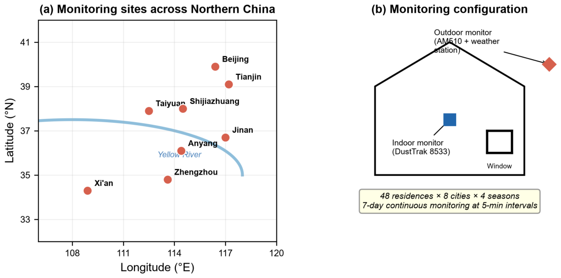
Figure 2.
Distribution of indoor (blue) and outdoor (red) PM2.5 concentrations (a) by city and (b) by season. Boxes show median and IQR; whiskers show 10th–90th percentiles. Dashed line: WHO 24-h guideline (35 μg m⁻³); dotted line: WHO AQG (15 μg m⁻³). Note the logarithmic y-axis.
Figure 2.
Distribution of indoor (blue) and outdoor (red) PM2.5 concentrations (a) by city and (b) by season. Boxes show median and IQR; whiskers show 10th–90th percentiles. Dashed line: WHO 24-h guideline (35 μg m⁻³); dotted line: WHO AQG (15 μg m⁻³). Note the logarithmic y-axis.
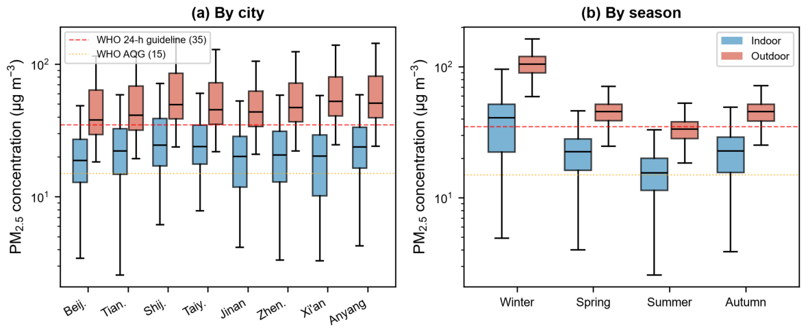
Figure 3.
Diurnal patterns: (a) indoor PM2.5 by season; (b) indoor PM2.5 by indoor source category; (c) window-open fraction by season. Shaded bands in (a) indicate typical meal-preparation hours.
Figure 3.
Diurnal patterns: (a) indoor PM2.5 by season; (b) indoor PM2.5 by indoor source category; (c) window-open fraction by season. Shaded bands in (a) indicate typical meal-preparation hours.
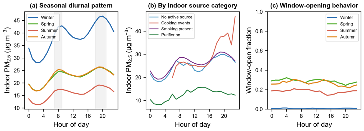
Figure 4.
Indoor vs. outdoor PM2.5 concentrations by season with linear regression lines. The dashed 1:1 line is shown for reference.
Figure 4.
Indoor vs. outdoor PM2.5 concentrations by season with linear regression lines. The dashed 1:1 line is shown for reference.
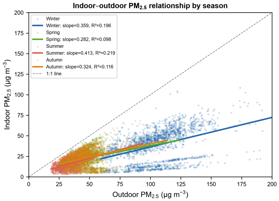
Figure 5.
(a) Building-specific infiltration factors (F_inf) by city; dashed line indicates the grand mean. (b) F_inf as a function of air change rate, colored by season. The dashed curve shows the theoretical relationship F_inf = P·a/(a + k) with P = 0.8 and k = 0.4 h⁻¹.
Figure 5.
(a) Building-specific infiltration factors (F_inf) by city; dashed line indicates the grand mean. (b) F_inf as a function of air change rate, colored by season. The dashed curve shows the theoretical relationship F_inf = P·a/(a + k) with P = 0.8 and k = 0.4 h⁻¹.
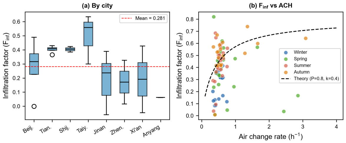
Figure 6.
Forest plot of multivariable regression coefficients for log(indoor PM2.5). Bars show 95% confidence intervals based on cluster-robust standard errors. Red: positive association; blue: negative association. * p < 0.1, ** p < 0.05, *** p < 0.01.
Figure 6.
Forest plot of multivariable regression coefficients for log(indoor PM2.5). Bars show 95% confidence intervals based on cluster-robust standard errors. Red: positive association; blue: negative association. * p < 0.1, ** p < 0.05, *** p < 0.01.
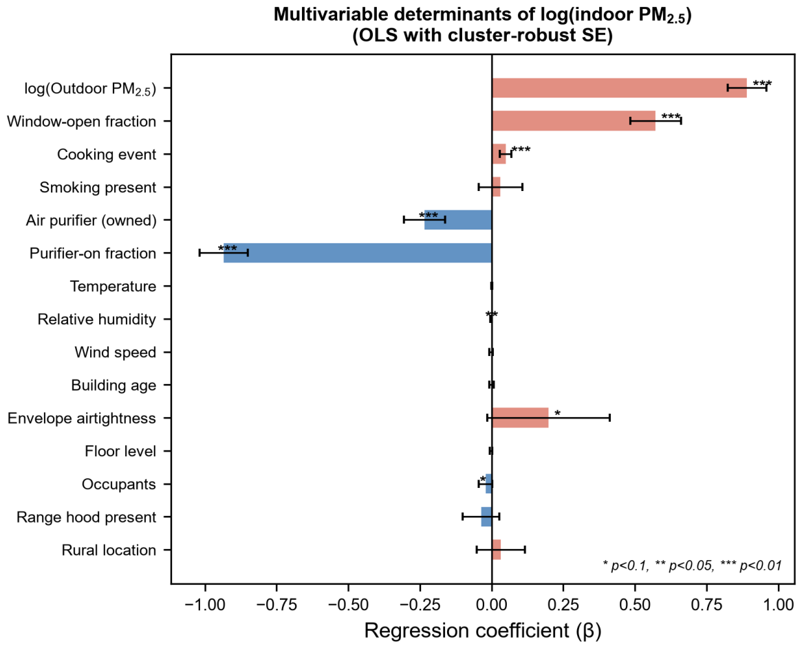
Figure 7.
Source apportionment of indoor PM2.5: (a) by season; (b) by city. Blue: outdoor origin; red: indoor origin.
Figure 7.
Source apportionment of indoor PM2.5: (a) by season; (b) by city. Blue: outdoor origin; red: indoor origin.
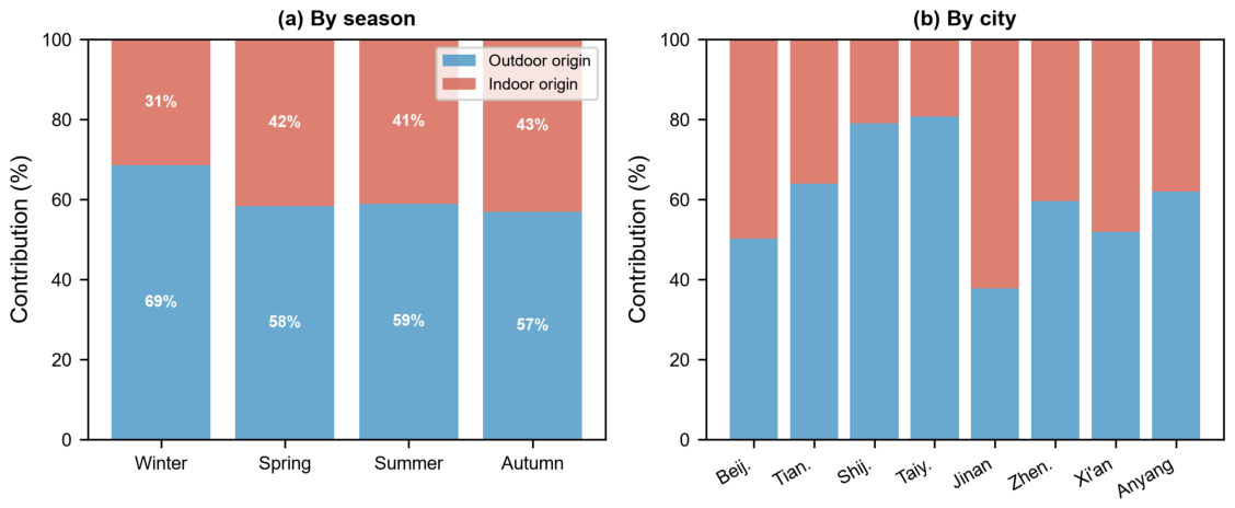
Figure 8.
Pearson correlation matrix of key variables. Color intensity and annotations show r values.
Figure 8.
Pearson correlation matrix of key variables. Color intensity and annotations show r values.
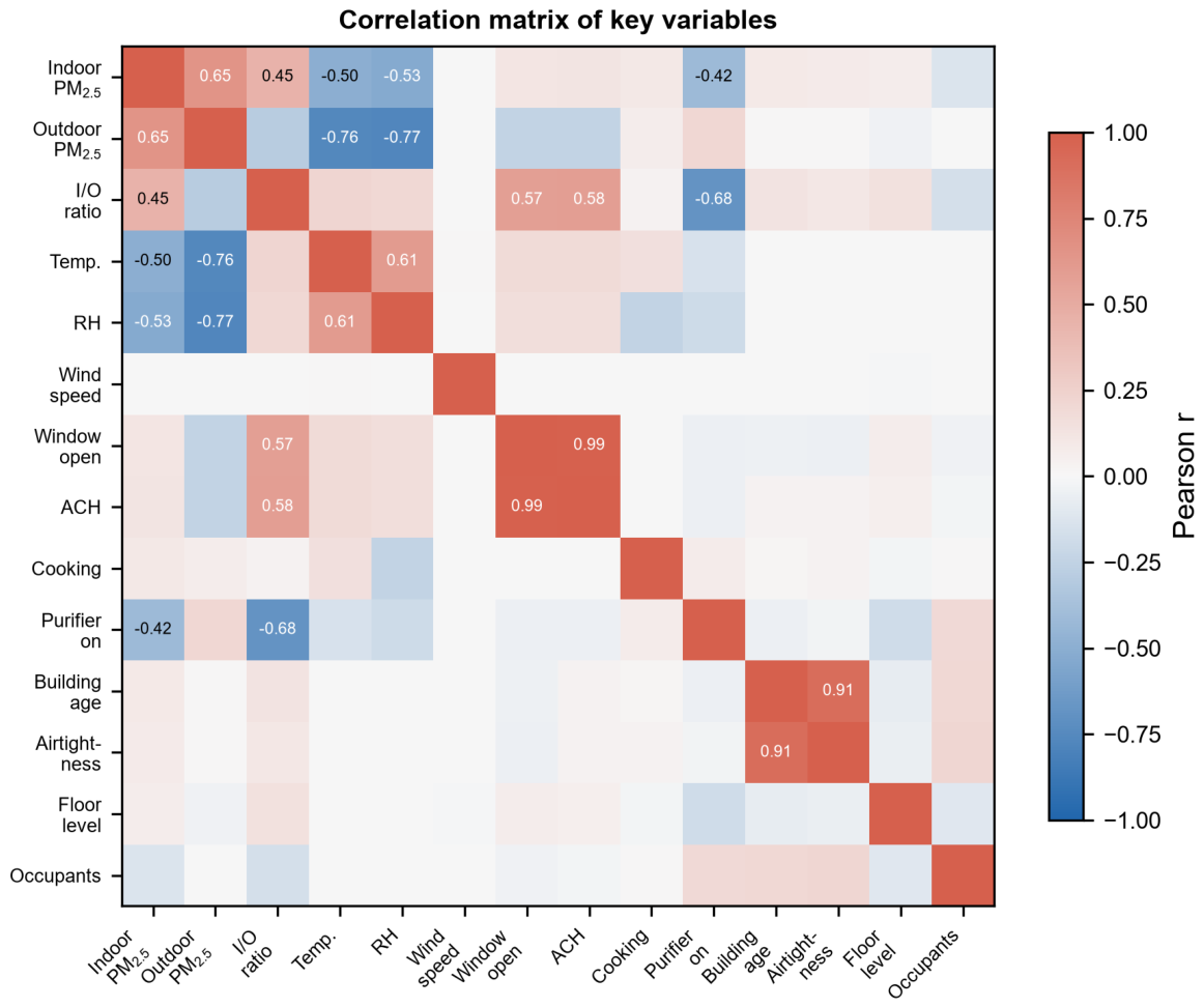

Table 1.
Summary of building and household characteristics (n = 48).
| Characteristic | Category | n | % |
| Building age | ≤10 years | 14 | 29.2 |
| 11–20 years | 20 | 41.7 | |
| >20 years | 14 | 29.2 | |
| Floor area | <80 m² | 12 | 25.0 |
| 80–110 m² | 24 | 50.0 | |
| >110 m² | 12 | 25.0 | |
| Heating type | District heating | 22 | 45.8 |
| Natural gas | 12 | 25.0 | |
| Electric heat pump | 7 | 14.6 | |
| Coal (rural) | 7 | 14.6 | |
| Kitchen type | Closed kitchen | 34 | 70.8 |
| Open kitchen | 14 | 29.2 | |
| Range hood | Present | 41 | 85.4 |
| Air purifier | Present | 17 | 35.4 |
| Smoking | None | 26 | 54.2 |
| Occasional | 15 | 31.2 | |
| Regular | 7 | 14.6 | |
| Location | Urban | 41 | 85.4 |
| Rural | 7 | 14.6 |
Table 2.
Descriptive statistics of indoor and outdoor PM2.5 concentrations by city (all seasons combined).
Table 2.
Descriptive statistics of indoor and outdoor PM2.5 concentrations by city (all seasons combined).
| City | Indoor mean±SD | Indoor median | Indoor P95 | Outdoor mean | Outdoor median | I/O median | n |
| Beijing | 21.5 ± 11.9 | 18.7 | 44.7 | 49.2 | 38.0 | 0.50 | 4032 |
| Tianjin | 24.9 ± 13.4 | 22.1 | 50.8 | 52.5 | 41.1 | 0.50 | 4032 |
| Shijiazhuang | 29.7 ± 17.1 | 24.5 | 64.6 | 64.8 | 49.5 | 0.50 | 4032 |
| Taiyuan | 28.1 ± 14.3 | 23.9 | 61.3 | 56.6 | 45.2 | 0.50 | 4032 |
| Jinan | 20.9 ± 10.5 | 20.1 | 39.6 | 51.9 | 43.6 | 0.40 | 4032 |
| Zhengzhou | 23.7 ± 14.4 | 20.6 | 51.5 | 58.0 | 47.2 | 0.50 | 4032 |
| Xi’an | 23.2 ± 16.6 | 20.3 | 57.6 | 64.1 | 52.5 | 0.40 | 4032 |
| Anyang | 27.1 ± 15.5 | 23.8 | 59.2 | 64.0 | 50.9 | 0.50 | 4032 |
| All | 24.9 ± 14.7 | 21.8 | 54.6 | 57.6 | 45.9 | 0.47 | 32256 |
Table 3.
Multivariable OLS regression results for log(indoor PM2.5) with cluster-robust standard errors (n = 32,256 hourly observations, 48 clusters).
Table 3.
Multivariable OLS regression results for log(indoor PM2.5) with cluster-robust standard errors (n = 32,256 hourly observations, 48 clusters).
| Season | P (penetration) | k (h⁻¹) | ACH (h⁻¹) | F_inf | R² |
| Winter | 0.80 | 0.67 (0.55–1.89) | 0.51 | 0.34 (0.17–0.40) | 0.84 |
| Spring | 0.80 | 0.58 (0.39–0.90) | 0.57 | 0.41 (0.24–0.48) | 0.39 |
| Summer | 0.80 | 0.44 (0.33–0.60) | 0.52 | 0.41 (0.38–0.50) | 0.42 |
| Autumn | 0.80 | 0.39 (0.23–0.52) | 0.53 | 0.48 (0.41–0.57) | 0.44 |
Table 4.
Multivariable OLS regression results for log(indoor PM2.5) with cluster-robust standard errors (n = 32,256 hourly observations, 48 clusters).
Table 4.
Multivariable OLS regression results for log(indoor PM2.5) with cluster-robust standard errors (n = 32,256 hourly observations, 48 clusters).
| Variable | β | SE | z | p | 95% CI |
| log(Outdoor PM2.5) | 0.891 | 0.034 | 26.18 | <0.001 | 0.824, 0.958 |
| Window-open fraction | 0.572 | 0.045 | 12.59 | <0.001 | 0.483, 0.661 |
| Cooking event | 0.049 | 0.010 | 4.71 | <0.001 | 0.028, 0.069 |
| Smoking present | 0.031 | 0.039 | 0.81 | 0.418 | −0.044, 0.107 |
| Air purifier (owned) | −0.234 | 0.037 | −6.35 | <0.001 | −0.306, −0.162 |
| Purifier-on fraction | −0.935 | 0.043 | −21.63 | <0.001 | −1.019, −0.850 |
| Temperature | 0.0004 | 0.001 | 0.43 | 0.665 | −0.001, 0.002 |
| Relative humidity | −0.002 | 0.001 | −2.10 | 0.036 | −0.003, −0.000 |
| Wind speed | −0.002 | 0.003 | −0.67 | 0.503 | −0.007, 0.003 |
| Building age | −0.0003 | 0.004 | −0.08 | 0.938 | −0.009, 0.008 |
| Envelope airtightness (n50) | 0.199 | 0.109 | 1.83 | 0.068 | −0.015, 0.414 |
| Floor level | −0.002 | 0.002 | −0.75 | 0.452 | −0.006, 0.002 |
| Occupants | −0.021 | 0.012 | −1.71 | 0.088 | −0.045, 0.003 |
| Range hood present | −0.037 | 0.033 | −1.12 | 0.261 | −0.101, 0.027 |
| Rural location | 0.032 | 0.043 | 0.74 | 0.460 | −0.053, 0.116 |
Table 5.
Indoor PM2.5 exceedance rates and estimated daily intake by city.
| City | WHO 15 μg/m³ exceedance | CN 35 μg/m³ exceedance | Daily intake (μg/day) |
| Beijing | 64.2% | 13.8% | 206 |
| Tianjin | 74.1% | 21.2% | 239 |
| Shijiazhuang | 80.9% | 29.4% | 285 |
| Taiyuan | 87.1% | 24.5% | 270 |
| Jinan | 63.7% | 10.7% | 201 |
| Zhengzhou | 69.5% | 20.7% | 227 |
| Xi’an | 60.7% | 17.8% | 223 |
| Anyang | 78.9% | 23.2% | 260 |
| All | 72.4% | 20.2% | 239 |
Disclaimer/Publisher’s Note: The statements, opinions and data contained in all publications are solely those of the individual author(s) and contributor(s) and not of MDPI and/or the editor(s). MDPI and/or the editor(s) disclaim responsibility for any injury to people or property resulting from any ideas, methods, instructions or products referred to in the content. |
© 2026 by the authors. Licensee MDPI, Basel, Switzerland. This article is an open access article distributed under the terms and conditions of the Creative Commons Attribution (CC BY) license (http://creativecommons.org/licenses/by/4.0/).
Copyright: This open access article is published under a Creative Commons CC BY 4.0 license, which permit the free download, distribution, and reuse, provided that the author and preprint are cited in any reuse.