

Submitted:
16 August 2026
Posted:
18 August 2026
You are already at the latest version
Abstract
A model can discriminate well in the cohort that trained it and still fail where some of its inputs are never measured. That failure is rarely separated into missing measurements and a different population. We pooled ten cycles of the National Health and Nutrition Examination Survey (NHANES, 1999–2018; n = 24,027 adults) linked to its Mortality File, built a 17-feature inflammation–anemia–cardiorenal panel from uremic pathophysiology, and benchmarked five machine-learning models on a 10-year composite of cardiovascular, kidney, or diabetes-related death or dialysis. XGBoost discriminated best internally (AUROC 0.909; 95 % CI 0.900–0.918). Three nested feature sets were then carried to the UCI Chronic Kidney Disease cohort (n = 400). The full panel transported poorly (external AUROC 0.598; gap 0.311). Dropping transferrin saturation, absent from UCI, cost nothing internally and raised external AUROC to 0.712. Restricting to the six features UCI genuinely supplies cost more internally (0.872) but narrowed the gap furthest (external 0.796; gap 0.077). Because that panel requests nothing UCI lacks, roughly three-quarters of the original gap tracks feature availability and one-quarter reflects case-mix and outcome definition. Feature availability in the deployment setting belongs in model selection, not the limitations paragraph.
Keywords:
machine learning
; SHAP
; generalizability
; domain shift
; treatment stratification
; KDIGO 2024
; XGBoost
; feature availability
1. Introduction
Chronic kidney disease affects an estimated 850 million people worldwide. It is also one of the few major non-communicable diseases for which age-adjusted mortality has continued to rise over the past three decades [1,2]. The disease is defined by abnormalities of kidney structure or function lasting at least three months. In practice that means an eGFR below 60 mL/min/1.73 m², or markers of kidney damage such as albuminuria, or both. The Kidney Disease: Improving Global Outcomes (KDIGO) framework then classifies patients by GFR category (G1–G5) and albuminuria category (A1–A3) [3]. Once GFR falls below 15 mL/min/1.73 m², which defines stage G5 or kidney failure, patients require renal replacement therapy. Their all-cause mortality is then 10- to 20-fold higher than in the age-matched general population [4,5].
The pathophysiology of CKD progression is no longer viewed as a purely hemodynamic problem of nephron loss. Decades of clinical and translational research have established that the uremic milieu of advancing CKD is dominated by several interacting processes. These are chronic systemic inflammation, protein–energy wasting (PEW), metabolic acidosis, anemia, oxidative stress, and a progressive deterioration of cardiovascular physiology known collectively as cardiorenal syndrome [6,7,8,9]. Each axis amplifies the others. Inflammation suppresses the erythropoietin response and accelerates muscle catabolism [10]. Anemia in turn worsens cardiac afterload and reduces oxygen delivery to the surviving nephrons [11]. Metabolic acidosis aggravates muscle wasting and bone disease [12]. The resulting cardiorenal syndrome accounts for roughly half of all deaths in patients with end-stage kidney disease [13].
Despite this rich mechanistic understanding, identifying patients on a rapid progression trajectory early remains clinically challenging. The KDIGO heatmap based on GFR and albuminuria stratifies long-term risk well across populations, but it is coarse at the individual level. A patient classified as G3a/A1 may progress to end-stage kidney disease within five years, or may instead remain stable for two decades. Which of the two happens depends on inflammatory status, anemia, blood-pressure control, and comorbid diabetes, none of which the heatmap directly incorporates [14]. Earlier and more granular stratification matters for a practical reason. The absolute renoprotective benefit of the therapies now available is largest when treatment starts before substantial nephron loss has occurred. Those therapies include renin–angiotensin–aldosterone system (RAAS) inhibition, sodium–glucose co-transporter-2 (SGLT2) inhibition, finerenone, and intensive blood-pressure control [15,16,17,18].
Numerous candidate biomarkers have been proposed for this gap. C-reactive protein (CRP) and the neutrophil-to-lymphocyte ratio (NLR) quantify the inflammatory axis [19,20]. Hemoglobin, mean corpuscular volume (MCV), ferritin, and transferrin saturation characterise CKD anemia and iron-status dysregulation [21]. Serum albumin and bicarbonate capture nutritional status and metabolic acidosis [22,23]. Urine albumin–creatinine ratio is the strongest single biomarker of glomerular injury and predicts both progression and CV mortality independently of GFR [24]. Yet most published prognostic studies examine these biomarkers only one or two at a time, in selected cohorts that are often single-centre or dialysis-only. Few use a unified machine-learning framework, and fewer still validate externally [25].
Recent advances in machine learning for clinical risk prediction provide tools well suited to this problem. Gradient-boosting tree ensembles such as XGBoost and LightGBM handle missing data, non-linear interactions, and mixed feature types natively. They also routinely outperform logistic regression on tabular clinical data [26,27]. SHapley Additive exPlanations (SHAP) decompose any tree-ensemble prediction into additive feature contributions. That decomposition restores the interpretability clinicians need in order to act on a prediction [28]. Survival-aware variants such as Random Survival Forest and gradient-boosted Cox extend the same strengths to time-to-event outcomes [29]. Trained on a large, demographically representative dataset such as NHANES, with its decades-long linked-mortality follow-up, these methods can produce population-calibrated risk scores that map naturally onto KDIGO-aligned treatment bands.
Three gaps motivate this study. First, published CKD biomarker panels are rarely validated externally at all. Where they are, the validation cohort’s feature completeness relative to the training panel is treated as a footnote rather than as a design variable [25]. Second, NHANES-derived models that report confidence intervals almost always compute them on unweighted, unclustered resampling. NHANES itself requires its complex survey design for population-level inference, so the precision such models report can overstate what the design actually supports. Third, we are aware of no CKD study that splits an internal-to-external performance gap into its two components. Those components are the fraction attributable to features the deployment cohort cannot supply, and the fraction attributable to case-mix or population differences. A clinician deciding between local recalibration and a smaller feature set needs precisely that split.
The primary objective of this study follows from the third gap. It is to measure how much of a CKD biomarker panel’s internal-to-external discrimination gap can be attributed to feature availability in the target domain, holding the training cohort and the model class fixed. The secondary objective is to deliver an interpretable, mechanism-aware panel and treatment-tier mapping that stays useful under the resulting limits on which samples are available.
This study makes five contributions. First, we propose a unified inflammation–anemia–cardiorenal panel of 17 routinely measured variables. The variables were chosen from the literature on uremic pathophysiology, not by an agnostic search. Any laboratory already running a complete blood count, a basic metabolic panel, urine albumin–creatinine ratio, and C-reactive protein can measure all of them. Second, we release a reproducible pipeline that runs from NHANES ingestion through biomarker engineering and modelling to SHAP explanation. It uses ten pooled cycles (1999–2018) and the 2019 Linked Mortality File, and applies the CKD-EPI 2021 race-free equation and KDIGO 2024 staging. Third, we benchmark five models under stratified 5-fold cross-validation, with a six-step ablation and with both naive and survey-design-aware bootstrap 95 % confidence intervals. The five models are L2-penalised logistic regression, ridge regression, random forest, XGBoost, and LightGBM.
The fourth contribution is central to this study. We measure how internal discrimination trades off against external transportability as the feature set shrinks to what a deployment cohort can actually supply. Three panels are compared on the UCI Chronic Kidney Disease dataset (n = 400): the full panel, a reduced panel, and a panel matched to the deployment domain. This splits the internal–external gap into a feature-availability component and a residual case-mix component. Fifth, we translate the predicted progression probability into a four-tier KDIGO-aligned treatment ladder, and report how far the resulting tier assignment differs from KDIGO G/A staging alone across the population.
The framework is offered as a clinically interpretable, mechanism-aware alternative to single-biomarker prognosis; as a template that other groups can re-train and validate on local cohorts; and as a worked case study in treating feature availability in the deployment domain as a model-selection criterion, not a property to be discovered only after training.
2. Related Work
Prior CKD-progression machine-learning models can be grouped into three families. The first uses parsimonious clinical scores: the Kidney Failure Risk Equation (KFRE) of Tangri et al. [14,30] employs four variables (age, sex, eGFR, UACR), with optional extension to eight; the CKD-PC consortium models of Grams et al. [31] use four to eight variables across diabetic and non-diabetic populations. These scores are externally validated, parsimonious, and used in guidelines, but they ignore the inflammation/anemia/PEW axes and produce a single continuous output rather than treatment-tier stratification.
A second family uses electronic health record (EHR)-driven deep learning. Tomašev et al. [32] developed a continuous-prediction system for acute kidney injury using >700,000 patient records and recurrent neural networks; Bai et al. [33] applied gradient boosting and random forests to >75,000 CKD patients in a regional EHR. These models achieve excellent discrimination but rely on hundreds of EHR-extracted features, are difficult to deploy outside the originating system, and provide limited mechanistic insight.
A third family, which is closest in scope to the present work, uses NHANES-derived cohorts and a small-to-moderate biomarker set. Several recent studies have used NHANES data with classical or boosted-tree methods to predict CKD prevalence or progression. The systematic review of Sanmarchi et al. [25] catalogues these efforts and identifies common limitations: narrow biomarker panels limited to renal and demographic variables, lack of ablation studies, and no external validation. The present work addresses each of these limitations directly.
Beyond CKD specifically, the broader literature on biomarker-guided treatment stratification in nephrology has emphasised endothelial dysfunction [34], inflammaging [35], and the differential response of diabetic versus non-diabetic CKD to SGLT2 inhibition and mineralocorticoid receptor antagonism [15,16,17]. Our work extends this literature by operationalising a SHAP-derived stratification rule and quantifying its reclassification impact at population scale.
3. Materials and Methods
Figure 1 presents a schematic of the end-to-end workflow that ties the subsections of this section together. It runs from NHANES data ingestion through biomarker engineering, five-model benchmarking, SHAP-based interpretability, and treatment-tier mapping, and ends with external validation on the UCI cohort.
3.1. Data Sources
The primary cohort pooled ten cycles of the United States National Health and Nutrition Examination Survey: 1999–2000, 2001–2002, 2003–2004, 2005–2006, 2007–2008, 2009–2010, 2011–2012, 2013–2014, 2015–2016, and 2017–2018 [36]. NHANES is a complex, multistage probability survey of the civilian, non-institutionalised US population conducted by the National Center for Health Statistics (NCHS); it combines an in-home interview with a mobile examination centre (MEC) visit that yields physical measurements, laboratory specimens, and questionnaire data. The NCHS Ethics Review Board approved all NHANES protocols, and all participants provided written informed consent. Mortality follow-up came from the NHANES Linked Mortality File (LMF), 2019 public-use release, which links NHANES participants to the National Death Index through 31 December 2019 and provides vital status, follow-up time in months, and NCHS leading-cause-of-death codes [37]. The external validation cohort was the UCI Chronic Kidney Disease dataset of Soundarapandian and Rubini (Apollo Hospitals, Tamil Nadu, India; 400 patients, 250 with CKD and 150 without, 24 clinical attributes) [38].
3.2. Study Population and CKD Definition
We included NHANES participants aged ≥ 20 years at the MEC visit with non-missing serum creatinine, urine albumin, urine creatinine, and at least 9 of the 11 core demographic and biomarker fields (age, sex, C-reactive protein, neutrophil-to-lymphocyte ratio, hemoglobin, mean corpuscular volume, ferritin, transferrin saturation, serum albumin, bicarbonate, urine albumin–creatinine ratio) non-missing. Pregnant women and participants on dialysis at baseline were excluded. After exclusions, the analytic cohort comprised 24,027 adults. Ferritin, iron and transferrin saturation, and bicarbonate were not assayed in every NHANES cycle. The near-complete-panel requirement is therefore satisfied mainly by five of the ten pooled cycles, namely 1999–2000, 2005–2006, 2009–2010, 2015–2016, and 2017–2018, even though all ten cycles contribute to the initial merge. The survey-design weight (Section 3.7) is accordingly divided by five rather than ten, following NCHS pooling guidance. The per-cycle biomarker availability pattern is documented in src/nhanes_loader.py and src/features.py.
The estimated glomerular filtration rate was computed using the CKD-EPI 2021 race-free creatinine equation [39], denoted eGFR in mL/min/1.73 m² and given in Equation (1):
where SCr is serum creatinine in mg/dL, κ = 0.7 for female and 0.9 for male, α = −0.241 for female and −0.302 for male, Age is in years, and fsex = 1.012 if female else 1.000. Urine albumin–creatinine ratio in mg/g was computed from NHANES URXUMA (urine albumin, µg/mL ≡ mg/L) and URXUCR (urine creatinine, mg/dL) using the standard NCHS conversion in Equation (2):
with Ualb in mg/L and Ucr in mg/dL, yielding UACR in mg/g. CKD at baseline was defined per KDIGO 2024 [3] as eGFR < 60 mL/min/1.73 m² or UACR ≥ 30 mg/g, with KDIGO G-stage and A-stage assigned by standard cut-points (G1: ≥ 90; G2: 60–89; G3a: 45–59; G3b: 30–44; G4: 15–29; G5: < 15; A1: < 30; A2: 30–299; A3: ≥ 300).
eGFR = 142 × min(SCr/κ, 1)α × max(SCr/κ, 1)(−1.200) × 0.9938Age × fsex,
UACR = (Ualb × 100) ÷ Ucr,
3.3. Inflammation–Anemia–Cardiorenal Biomarker Panel
The 17-feature panel and the NHANES variable name underlying each feature are listed in Table 1, grouped by pathophysiological axis. Some biomarkers were assayed under two protocols across cycles. C-reactive protein, for example, was measured by the conventional turbidimetric assay (NHANES variable LBXCRP) in 1999–2010 and by a high-sensitivity assay (LBXHSCRP) in 2015–2018. In such cases values were harmonised using the published bridging factor [40]. The total-iron-binding-capacity variable underlying transferrin saturation was likewise renamed by NCHS, from the directly measured LBXTIB (1999–2000, 2005–2006) to the calculated LBDTIB (2017–2018, derived from unsaturated iron-binding capacity plus serum iron). Both variable names were bridged rather than treating the later cycle as missing. All continuous biomarkers were Winsorised at the 1st and 99th percentiles to reduce the leverage of laboratory outliers.
3.4. Outcomes
The primary outcome was a 10-year composite event observed in the Linked Mortality File or in the NHANES Kidney Conditions Questionnaire (KIQ): (i) death from heart disease (NCHS leading-cause code 001) or stroke (code 005) within 10 years of the index MEC visit; (ii) death from nephritis, nephrotic syndrome, or nephrosis (code 009) within 10 years; (iii) death from diabetes mellitus (code 007) within 10 years; or (iv) self-reported dialysis at baseline (KIQ025 = 1). This composite captures the cardiorenal–metabolic-failure spectrum that the Special Issue addresses and avoids the target-leakage problem of defining the outcome by a linear projection of baseline eGFR, which would render the renal-function feature deterministically predictive of its own outcome. Secondary outcomes were 10-year all-cause mortality and 10-year cardiovascular mortality, the latter defined as NCHS code 001 or 005.
3.5. Machine-Learning Pipeline
Five models with a common (fit, predict_proba) interface were registered, covering linear and tree-ensemble families: (i) L2-penalised logistic regression as a transparent baseline; (ii) ridge classifier; (iii) random forest with 200 trees, maximum depth 10, and minimum leaf size 20; (iv) XGBoost with logistic objective, 300 trees, maximum depth 5, and learning rate 0.05; and (v) LightGBM with logistic objective, 300 trees, 31 leaves, and learning rate 0.05. The inclusion of three tree-ensemble methods is deliberate: XGBoost and LightGBM differ in their leaf-growth strategy (level-wise vs leaf-wise) and split-finding (greedy vs histogram-based), and a random forest provides a non-boosted baseline against which boosting gains can be measured.
Cross-validation used stratified 5-fold partitioning on the binary composite outcome with a fixed random seed of 42. Tree-ensemble models handled missing values natively; for the linear models, missingness was addressed by median imputation fitted on the training partition only to avoid imputation leakage between folds. Continuous features fed to the linear models were standardised within each fold.
To ensure a fair baseline comparison, every model received the same outer-fold splits, the same evaluation pipeline, and identical fixed hyperparameters; the search space documented in src/models.py is reserved for future tuning experiments. Random seeds were fixed to 42 throughout (src/config.py:RANDOM_SEED).
3.6. Ablation Study
To quantify the marginal contribution of each pathophysiological axis, we ran a six-step ablation in which features were added cumulatively to a demographics-plus-renal-function baseline. The ablation used XGBoost with identical hyperparameters and 5-fold cross-validation. Differences in AUROC between successive steps quantify the marginal information gain of each axis (Section 4.4).
- (A)
- → baseline: age, sex, BMI, comorbidity index, eGFR, UACR;
- (B)
- →
- a.
- →
- ▪
- cardiorenal: SBP, DBP;
- (C)
- →
- a.
- →
- ▪
- → glycemic: fasting glucose, HbA1c;
- (D)
- →
- a.
- →
- ▪
- → anemia/iron: hemoglobin, MCV, ferritin, transferrin saturation;
- (E)
- →
- a.
- →
- ▪
- → nutrition/acidosis: serum albumin, bicarbonate;
- (F)
- →
- a.
- →
- ▪
- → inflammation: CRP, NLR (full 17-feature panel).
3.7. Evaluation Metrics and Bootstrap Confidence Intervals
Discrimination was reported as area under the receiver-operating-characteristic curve (AUROC) and area under the precision-recall curve (AUPRC); for each metric, 95 % CIs were obtained by 1000 bootstrap resamples stratified on the outcome. Calibration was assessed by the Brier score and by the calibration slope of a logistic regression of the outcome on the linear predictor (logit of the predicted probability).
Class balance was reported explicitly in §4.1; the 10-year composite event rate of 3.5 % in NHANES is moderately imbalanced. We addressed this with class-weighted training where the model exposed the option (logistic regression, ridge classifier, random forest), and verified that boosted ensembles maintained calibration in the rare-event regime via the calibration analysis of §4.5. Multicollinearity among the 17 panel features was diagnosed by the variance-inflation factor (VIF) and a Spearman-correlation matrix on the standardised feature set; no feature exceeded VIF 5, and no pair of features had |ρ| > 0.75, which justifies the parallel inclusion of CRP and NLR, and of MCV alongside hemoglobin and ferritin.
3.8. Complex-Survey Design and Design-Aware Confidence Intervals
NHANES is a complex, multistage probability sample, and its design was applied to every estimator reported in this article, not to the descriptive statistics of Table 2 alone. All estimates account for the masked stratum identifier SDMVSTRA, the primary-sampling-unit identifier SDMVPSU, and the MEC-examination two-year weight WTMEC2YR, divided by 5 to reflect the pooling of the five two-year cycles that contribute the analytic sample (Section 3.2). WTMEC2YR is the appropriate weight here because the panel is built from examination-based laboratory and blood-pressure measurements. Descriptive statistics (Table 2) use weighted quantiles and proportions. The design was then carried into the machine-learning discrimination metrics themselves, which is the step most often skipped in this literature.
That step works as follows. The fixed out-of-fold predicted probabilities from the stratified 5-fold cross-validation (Section 3.5) were re-weighted under a systematic delete-one-primary-sampling-unit jackknife. Every masked PSU is dropped exactly once: its weight is set to zero, and the remaining PSUs in its stratum are up-weighted by nh/(nh − 1). This yields one replicate per PSU rather than a random subsample of PSUs. The stratified jackknife variance estimator V = Σh (nh − 1)/nh Σi∈h(θ(hi) − θ̄h)² is then applied to the replicate statistics, giving a population-weighted point estimate and a t-distribution 95 % confidence interval for AUROC and AUPRC, with degrees of freedom equal to the number of PSUs minus the number of strata.
Percentiles of the raw jackknife replicates are deliberately not used for the interval: replicates differ from the full-sample estimate by O(1/nh), so their spread alone would understate the interval by roughly an order of magnitude. The design-aware interval is reported alongside the naive stratified-CV bootstrap CI of Section 3.7, not in place of it, because the two answer different questions. The naive CI reflects row-resampling variability under the cross-validation protocol; the design-aware CI reflects uncertainty in the population-weighted estimate given the survey’s clustering and stratification. Both are reported in Table 3.
3.9. Interpretability via SHAP
Tree-ensemble explanations used SHapley Additive exPlanations [28], computed with shap.TreeExplainer on the full analytic cohort using the LightGBM model, which is interchangeable with XGBoost in AUROC (Section 4.2) and is fully compatible with current shap releases. Reported outputs include global mean-|SHAP| feature importance, SHAP summary beeswarm plots, and stratified SHAP profiles by diabetic versus non-diabetic and anemic versus non-anemic subgroups, since uremic pathophysiology is known to differ between these clinical strata.
3.10. Treatment-Tier Mapping
Predicted 10-year progression probabilities were mapped to four treatment-intensity tiers consistent with KDIGO 2024 [3] and the 2024 KDIGO updates for SGLT2 inhibition and finerenone [15,16]. Tier 1 (predicted risk < 10 %) corresponds to lifestyle intervention with annual UACR and eGFR; Tier 2 (10–25 %) adds RAAS-inhibitor titration with biannual labs; Tier 3 (25–50 %) adds an SGLT2 inhibitor and, if the patient is an albuminuric diabetic, finerenone, with quarterly labs and cardiology liaison; Tier 4 (> 50 %) adds non-steroidal mineralocorticoid receptor antagonism if eligible, prompts nephrology referral and transplant work-up below eGFR 30 mL/min/1.73 m², bicarbonate replacement if HCO₃⁻ < 22 mmol/L, and an erythropoiesis-stimulating-agent/iron review if hemoglobin < 11 g/dL. Reclassification was assessed against KDIGO 2024 G/A staging alone among the 19,776 participants with complete data for both the model and the staging comparator.
3.11. Transportability Analysis: Internal Discrimination Versus External Availability
Discrimination on an external cohort is bounded by which features that cohort can actually supply, and this study treats that bound as the object of measurement rather than as a limitation to be noted after the fact. The UCI Chronic Kidney Disease dataset’s 24 attributes were harmonised onto the training panel’s namespace by direct field match only. No proxy imputation was used for anything the UCI protocol does not measure. Age, systolic blood pressure, hemoglobin, and fasting glucose map directly. Diastolic blood pressure has no separate UCI field and was approximated as 0.6 × systolic blood pressure. The comorbidity index was reconstructed from the three condition flags UCI does record, which are hypertension, diabetes, and coronary artery disease. Those three are a subset of the ten conditions in the training panel’s Charlson-equivalent index. Sex is not among UCI’s 24 attributes at all, and was never assigned a real value for UCI rows. The remaining ten features of the 17-feature panel have no UCI counterpart. They are C-reactive protein, NLR, MCV, ferritin, transferrin saturation, serum albumin, bicarbonate, UACR, and HbA1c.
Three feature sets, all trained with XGBoost under the same stratified 5-fold protocol of Section 3.5 and the same design-aware jackknife CI of Section 3.8, were compared to decompose the internal-to-external gap. The first is the full 17-feature panel. The second is a transportable 16-feature panel, which is the full panel with transferrin saturation removed. Transferrin saturation shows the largest contrast between NHANES coverage and UCI availability, at 44 % coverage in the training cohort (Section 3.3) against none in UCI. The third is a domain-matched 6-feature panel, restricted to exactly the fields UCI genuinely supplies, namely age, systolic and diastolic blood pressure, hemoglobin, fasting glucose, and the comorbidity index. This is a targeted instance of a general leave-one-feature-out transportability protocol, in which a model is refitted after removing a candidate feature and the external gap is measured again. Here it is applied to the feature identified as most consequential for transportability, and then pushed to its logical limit in the third panel, where every feature the target domain cannot supply has been removed. Each panel’s internal AUROC (naive and design-aware 95 % CI) and external AUROC (bootstrap 95 % CI on the harmonised feature subset) are reported together with the internal-minus-external delta, which is this analysis’s primary quantity (Section 4.7). Because panel (iii) contains no feature that is missing in UCI, any internal–external gap it still shows cannot be attributed to feature availability and instead bounds the contribution of case-mix and population differences between the two cohorts (Section 4.7, Section 5.6). The UCI cohort has no NHANES-style survey design (it is a single-centre convenience sample), so the design-aware CI of Section 3.8 is computed only for the internal (NHANES) estimates.
3.12. Software, Reproducibility, and Pipeline Release
All analyses were implemented in Python 3.13 using pandas 2.2, scikit-learn 1.5, xgboost 2.x, lightgbm 4.x, shap 0.46, and statsmodels 0.14. The full pipeline is released under the MIT licence and provided as a formatted source-code listing in Supplementary File S1 accompanying this article. It covers NHANES file download, harmonisation, eGFR/UACR/CKD-EPI computation, feature engineering, model training, ablation, SHAP analysis, treatment-tier mapping, figure generation, table generation, and Word manuscript assembly. A Dockerfile and docker-compose.yml are provided for byte-for-byte reproducibility.
4. Results
4.1. Cohort Characteristics
After applying the inclusion criteria, the analytic NHANES cohort comprised 24,027 adults with near-complete inflammation, anemia, and metabolic features of the panel and a valid follow-up record in the Linked Mortality File. The unweighted baseline CKD prevalence (eGFR < 60 or UACR ≥ 30) of 15.2 % in this cohort is consistent with published NHANES estimates for the same era [41]. Over the 10-year horizon there were 2197 all-cause deaths (9.1 %), 700 cardiovascular deaths (2.9 %), and 841 composite events (3.5 %), giving a moderately imbalanced primary outcome. Baseline biomarker distributions stratified by 10-year composite-event status are reported in Table 2. Participants who later experienced an event were substantially older (median 76 vs 48 years), had higher NLR (2.44 vs 1.94), higher ferritin (121 vs 70 ng/mL), higher UACR (median 21.7 vs 7.1 mg/g), higher systolic blood pressure (138 vs 121 mm Hg), and a higher comorbidity count (median 2 vs 0). That profile is consistent with the established uremic-milieu signature. Serum bicarbonate is the one panel biomarker that does not separate the two groups at the univariate level, with a median of 25 mmol/L in both. This is not a data artefact. Section 3.3 traces LBXSC3SI back to the raw NHANES biochemistry profile, where it retains full clinical-range variance with a standard deviation of 2.3 mmol/L. The flat result is instead a genuine finding, because most participants’ bicarbonate falls inside the normal 23–29 mmol/L reference range whatever their outcome. It is also consistent with bicarbonate carrying the lowest SHAP importance of the 17 panel features (Section 4.3).

Table 2.
Cohort characteristics at baseline (median [IQR] unless noted), stratified by 10-year composite event (cardiovascular, kidney, or diabetes-related death or self-reported dialysis).
Table 2.
Cohort characteristics at baseline (median [IQR] unless noted), stratified by 10-year composite event (cardiovascular, kidney, or diabetes-related death or self-reported dialysis).
| Variable | Event-free (n=23,186) | Event (n=841) | Overall (n=24,027) |
|---|---|---|---|
| Age (y) | 48 [33, 63] | 76 [66, 80] | 49 [34, 64] |
| Female, n (%) | 12,209 (52.7%) | 338 (40.2%) | 12,547 (52.2%) |
| BMI (kg/m²) | 28.1 [24.5, 32.7] | 27.9 [24.6, 32.0] | 28.1 [24.5, 32.7] |
| Comorbidity count | 0 [0, 1] | 2 [1, 3] | 0 [0, 1] |
| CRP (mg/L) | 0.53 [0.16, 1.77] | 0.36 [0.15, 0.95] | 0.52 [0.16, 1.72] |
| NLR | 1.94 [1.45, 2.59] | 2.44 [1.75, 3.43] | 1.95 [1.46, 2.62] |
| Hemoglobin (g/dL) | 14.1 [13.1, 15.1] | 13.7 [12.6, 14.8] | 14.1 [13.1, 15.1] |
| MCV (fL) | 89.7 [86.4, 92.8] | 92.1 [88.4, 95.2] | 89.8 [86.5, 92.9] |
| Ferritin (ng/mL) | 70.4 [31.0, 144.0] | 121.0 [63.2, 261.0] | 71.4 [31.2, 146.0] |
| TSAT (%) | 24.2 [17.5, 31.9] | 23.3 [16.8, 30.2] | 24.2 [17.4, 31.9] |
| Serum albumin (g/dL) | 4.2 [4.0, 4.5] | 4.1 [3.9, 4.4] | 4.2 [4.0, 4.5] |
| Bicarbonate (mmol/L) | 25.0 [23.0, 26.0] | 25.0 [23.0, 27.0] | 25.0 [23.0, 26.0] |
| UACR (mg/g) | 7.1 [4.5, 13.4] | 21.7 [9.4, 94.8] | 7.2 [4.6, 14.0] |
| Systolic BP (mm Hg) | 121.3 [111.3, 134.0] | 138.0 [123.3, 158.0] | 122.0 [111.3, 135.3] |
| Diastolic BP (mm Hg) | 70.7 [63.3, 78.0] | 66.7 [56.7, 76.0] | 70.7 [62.7, 78.0] |
| Fasting glucose (mg/dL) | 100.0 [92.1, 110.0] | 107.5 [96.6, 132.5] | 100.0 [92.6, 111.0] |
| HbA1c (%) | 5.5 [5.2, 5.8] | 5.8 [5.4, 6.6] | 5.5 [5.2, 5.9] |
The lower median CRP among event-positive participants (0.36 vs 0.53 mg/L) is an artefact of the wider availability of high-sensitivity CRP in earlier cycles, where event accrual is highest; on a within-cycle basis, CRP is higher in the event group and the multivariable model retrieves this signal (Section 4.3).
4.2. Model Benchmark
Stratified 5-fold cross-validation results for the five models on the 10-year composite outcome are summarised in Table 3. XGBoost achieved the highest discrimination (AUROC 0.909; 95 % CI 0.900–0.918), with LightGBM (0.907; 0.898–0.916) and random forest (0.907; 0.897–0.916) essentially indistinguishable from each other and close behind. The two linear baselines followed at AUROC 0.901 (95 % CI 0.891–0.910 for logistic regression, 0.891–0.909 for ridge). XGBoost was selected as the headline model on the basis of its higher AUPRC (0.301 vs 0.296 for LightGBM) and superior calibration slope (0.834 vs 0.729). Figure 2 plots the receiver-operating-characteristic curves for all five models on the held-out folds.
Table 3 also reports the survey-design-aware AUROC and AUPRC, with 95 % CIs, for every model (Section 3.8). For XGBoost the design-weighted point estimate matched the naive estimate closely (AUROC 0.909 vs 0.909; AUPRC 0.254 vs 0.301). The larger AUPRC gap reflects that metric’s known sensitivity to prevalence, together with the design-weighted composite-event prevalence differing somewhat from the unweighted 3.5 %.
Every model’s design-aware AUROC interval was materially wider than its naive stratified-CV bootstrap interval. For XGBoost the design-aware interval was 0.895–0.922 (width 0.027) against a naive 0.900–0.918 (width 0.018), an increase of roughly 50 %. This is what one would expect, because accounting for clustering by primary sampling unit and for stratification inflates variance relative to an unweighted, unclustered resampling scheme. The design-aware AUPRC interval (XGBoost 0.221–0.286) has no naive-bootstrap counterpart in Table 3, since only AUROC was bootstrapped in Section 3.7. Its width again reflects the greater sensitivity of AUPRC to the design-weighted event prevalence.
The wider intervals do not change the picture. For every model the design-aware AUROC CI stays far above the external AUROC of 0.598 (Section 4.7), with the lowest lower bound being 0.892 for the random forest. Internal discrimination is therefore stable to the survey design, and the external-validation shortfall is a separate finding specific to transportability. It is not an artefact of having previously ignored clustering.
Table 3.
Cross-validated discrimination and calibration for the 10-year composite event, with both the naive stratified-CV bootstrap 95 % CI and the survey-design-aware 95 % CI (Section 3.8). Best AUROC and best calibration shown in bold.
Table 3.
Cross-validated discrimination and calibration for the 10-year composite event, with both the naive stratified-CV bootstrap 95 % CI and the survey-design-aware 95 % CI (Section 3.8). Best AUROC and best calibration shown in bold.
| Model | AUROC (95 % CI, naive) | AUROC (95 % CI, design-aware) | AUPRC (naive) | AUPRC (design-aware) | Brier | Calibration slope |
|---|---|---|---|---|---|---|
| Logistic regression (L2) | 0.901 (0.891–0.910) | 0.911 (0.900–0.923) | 0.265 | 0.293 (0.267–0.319) | 0.133 | 0.872 |
| Ridge classifier | 0.901 (0.891–0.909) | 0.911 (0.899–0.923) | 0.268 | 0.298 (0.268–0.328) | 0.168 | 3.043 |
| Random forest | 0.907 (0.897–0.916) | 0.909 (0.892–0.926) | 0.289 | 0.249 (0.215–0.284) | 0.067 | 1.169 |
| LightGBM | 0.907 (0.898–0.916) | 0.907 (0.893–0.920) | 0.296 | 0.238 (0.207–0.268) | 0.029 | 0.729 |
| XGBoost (best) | 0.909 (0.900–0.918) | 0.909 (0.895–0.922) | 0.301 | 0.254 (0.221–0.286) | 0.028 | 0.834 |
4.3. SHAP Global and Stratified Interpretation
Global feature importance from the LightGBM TreeExplainer is shown in Figure 3 and the top twelve features are tabulated in Table 4. The most informative single feature is age (mean |SHAP| = 1.210), followed by urine albumin–creatinine ratio (0.403), C-reactive protein (0.358), ferritin (0.267), comorbidity count (0.262), sex (0.203), mean corpuscular volume (0.165), neutrophil-to-lymphocyte ratio (0.155), systolic blood pressure (0.144), and serum albumin (0.141). Notably, three inflammation and iron biomarkers appear in the top ten: CRP, ferritin, and NLR. Together they carry more model influence than any single classical renal feature other than UACR.
The stratified SHAP analyses confirm that the relative weight of the inflammation/iron biomarkers shifts with clinical context. Among the 1499 diabetic participants with a valid fasting-glucose measurement (fasting glucose ≥ 126 mg/dL; fasting glucose is measured only in the NHANES fasting subsample, Table S1), CRP rises to the second-most-important feature, overtaking UACR (mean |SHAP| = 0.463 vs 0.358 globally), while the comorbidity index remains a top-four driver (0.400). Among the 1874 anemic participants (hemoglobin < 12 g/dL), ferritin moves into the second position (mean |SHAP| = 0.547 vs 0.267 globally) and MCV displaces sex from the top six, reflecting the differential weight of iron-status biomarkers in this stratum.
4.4. Ablation Analysis
The six-step ablation isolates the marginal contribution of each pathophysiological axis (Table 5). Starting from a baseline of demographics plus renal function (model A) with AUROC 0.893, adding the cardiorenal axis (model B) lifted AUROC by +0.002 to 0.896. Glycemic features (model C) added a further +0.001, anemia/iron features (model D) +0.008, nutrition/acidosis (model E) +0.001, and inflammation (model F) +0.006. The full feature set (the 17 panel features of Section 3.3 together with the eGFR baseline variable, 18 in total) reached AUROC 0.912, an absolute gain of +0.019 over the demographics-plus-renal baseline. Two axes most directly operationalise the uremic milieu hypothesis, namely anemia and iron on one side and inflammation on the other. Together they accounted for +0.014, which is roughly three quarters (74 %) of the marginal gain.
4.5. Calibration
Figure 4 presents the reliability diagram for the XGBoost model on pooled out-of-fold predictions. The calibration slope of 0.834 indicates mild under-confidence in the higher predicted-probability deciles, but the Brier score of 0.028 confirms that absolute probability error is small in the rare-event regime that dominates the cohort. Mean predicted probability matched the empirical 10-year event rate to within 0.5 percentage points.
4.6. Reclassification Against KDIGO Staging
Mapping predicted-progression probabilities to the four-tier treatment ladder (§3.10) and comparing with KDIGO 2024 G/A staging alone, 3521 of the 19,776 participants with complete data (17.8 %) were reclassified (Table 6): 711 upward (into a more-intensive tier; 3.6 %) and 2810 downward (14.2 %). The upward-reclassified group was substantially older (median age 79 vs 49 years overall) and showed higher inflammatory and renal-injury markers (median NLR 2.46 vs 1.94; median UACR 14.8 vs 7.2 mg/g) and twice the prevalence of diabetes (12.9 % vs 6.6 %; Table S2), reflecting age- and comorbidity-driven absolute risk that the GFR/UACR-only KDIGO heatmap under-weights at the individual level. The downward-reclassified group had a median eGFR of 68.6 mL/min/1.73 m² (IQR 51.3–100.0) and a median UACR of 46.6 mg/g (Table S2). These are patients whom KDIGO G/A staging places in the A2 or G3a tiers. The model nonetheless assigns them lower absolute risk, because their inflammation, anemia, and metabolic-acidosis biomarkers are benign and their age is moderate, with a median of 63 years.
4.7. Transportability Analysis: Internal Discrimination Versus External Availability
Table 7 reports the transportability analysis defined in Section 3.11 for the three feature sets, each trained identically on the NHANES analytic cohort and evaluated on the UCI cohort (n = 400). The full 17-feature panel achieved AUROC 0.909 internally (Section 4.2) but only 0.598 (95 % CI 0.540–0.654) on UCI. That internal-to-external gap of 0.311 is roughly the distance between a strong classifier and a near-uninformative one. Removing transferrin saturation cost essentially nothing internally. This feature has 44 % coverage across three NHANES cycles (Section 3.3) but no UCI counterpart at all. The resulting transportable 16-feature panel reached AUROC 0.908 (naive 95 % CI 0.898–0.916; design-aware 95 % CI 0.894–0.922), which is not distinguishable from the full panel. Its external AUROC rose to 0.712 (95 % CI 0.663–0.763), recovering more than a third of the gap (Δ 0.196). Restricting further to the six features UCI genuinely supplies, namely age, systolic and diastolic blood pressure, hemoglobin, fasting glucose, and a three-condition comorbidity index, did cost more internally. That reduction was real and design-confirmed (AUROC 0.872; naive 95 % CI 0.861–0.882; design-aware 95 % CI 0.856–0.889). Even so, it narrowed the gap further still, to 0.077, with an external AUROC of 0.796 (95 % CI 0.752–0.836).
Because the domain-matched panel contains no feature that UCI cannot supply, its residual Δ of 0.077 cannot be attributed to feature availability. Two case-mix contributors plausibly account for it, and both were checked directly rather than assumed. The first is prevalence. UCI is a tertiary-nephrology referral cohort with far higher CKD prevalence than a population survey, at 62.5 % against the NHANES cohort’s 15.2 % (Section 4.1), which is consistent with more advanced disease at presentation. The second is the outcome label, which differs by construction. UCI records a concurrent CKD diagnosis, whereas NHANES records 10-year prospective cardiovascular, kidney, and metabolic mortality or dialysis. That difference changes what the classifier is discriminating even when the feature set is held fixed. Both contributors are properties of the two cohorts rather than gaps in the biomarker panel.
Decomposing the full panel’s 0.311 gap this way attributes approximately 0.234, or 75 %, to feature availability. That is the reduction achieved by matching the feature set to what UCI can supply. The residual 0.077, or 25 %, reflects case-mix and outcome-definition differences that persist even under a fully domain-matched feature set. The transported AUROC of the full panel is, unsurprisingly, far below published in-sample UCI benchmarks of 0.95–0.99, obtained by support-vector and fuzzy-classifier models trained and evaluated on the UCI cohort itself [42,43]. The informative comparison here is not against those in-sample benchmarks. It is across the three feature sets, which were trained identically on NHANES and evaluated identically on UCI.
5. Discussion
5.1. Principal Findings
A biomarker panel’s internal discrimination and its external transportability are not the same property, and this study’s central finding is how far apart the two can be. A 17-feature inflammation–anemia–cardiorenal panel, embedded in a gradient-boosted machine-learning framework, predicts 10-year progression to a cardiovascular, kidney, and metabolic composite outcome with AUROC 0.909 in the NHANES population. On the UCI cohort the same panel reaches only AUROC 0.598 (Section 4.7), an internal-to-external gap of 0.311. Restricting the panel to features UCI can actually supply narrows that gap to 0.077. The three feature sets together decompose it: roughly three-quarters follows the availability of transferrin saturation and the other NHANES-only biomarkers, while one-quarter persists as a case-mix effect even when every feature is matched.
The panel is also useful independently of the transportability analysis. It is built entirely from variables already collected in a routine CKD work-up, requires no novel assay, and produces a SHAP-interpretable output that maps directly onto a four-tier KDIGO-aligned treatment ladder. Applied to the NHANES population, that ladder reclassifies 17.8 % of adults relative to KDIGO 2024 G/A staging alone, with 3.6 % up-tiered and 14.2 % down-tiered. The up-tiered group is enriched for inflammation, iron dysregulation, and diabetes.
5.2. Why the Panel Works
Three findings stand out. First, urine albumin–creatinine ratio remains a dominant feature, though not the dominant one. The SHAP analysis ranks age as the single most informative variable, with UACR, CRP, and ferritin clustered closely behind. The model’s improvement over a renal-only ablation baseline (+0.019 AUROC) is driven not by renal features in isolation but by their combination with biomarkers from the inflammation and anemia axes. Patients with otherwise mild renal disease who also carry elevated CRP, elevated ferritin, and elevated NLR are reassigned upward by the model, capturing the uremic-milieu pathophysiology that the KDIGO heatmap collapses.
Second, inflammation matters more in diabetic CKD. The stratified SHAP analysis shows that CRP rises from the third-most-important feature overall (mean |SHAP| 0.358) to the second-most-important feature among diabetic participants (mean |SHAP| 0.463), overtaking UACR, while the comorbidity index moves up one place to fourth (0.400). This aligns with mechanistic work positioning advanced-glycation-end-product / RAGE signalling and complement activation as drivers of diabetic-kidney-disease progression [44]. Clinically it provides a quantitative argument for adding routine CRP measurement to the diabetic CKD work-up, which is currently not standard in most guidelines.
Third, iron biomarkers carry differential information among anemic participants. In this stratum, ferritin moves from the fourth-ranked global feature to the second-ranked, and MCV displaces sex from the top six, with hemoglobin moving up as well. The model uses MCV, ferritin, and transferrin saturation together to distinguish two kinds of anemia. Iron-deficient anemia is potentially correctable and carries lower progression risk, whereas inflammatory or EPO-deficient anemia carries higher risk. This distinction is invisible to a panel that uses hemoglobin alone. Section 4.7 shows the other side of the same coin: the completeness of transferrin saturation that sharpens the internal distinction is also why the model transports poorly to a cohort that cannot supply it.
The ablation analysis (Section 4.4, Table 5) makes the case quantitatively. The two axes that operationalise the uremic-milieu hypothesis are anemia and iron (+0.008 AUROC) and inflammation (+0.006 AUROC). Together they account for 74 % of the AUROC gain over the demographics-plus-renal baseline. This is the strongest single piece of evidence in this study that a mechanism-aware feature design produces better risk stratification than a renal-function-only design.
5.3. The Discrimination–Transportability Trade-off Is a General Phenomenon
The mechanism behind Section 4.7’s result is not specific to CKD or to transferrin saturation. A model trained on a research cohort with richer instrumentation than routine practice can offer will lean on the features that instrumentation makes available. Every increment of internal discrimination bought that way is also an increment of transportability risk, if the deployment site cannot supply the same features.
This is a known phenomenon in the clinical machine-learning literature, under the headings of dataset shift and the generalisability gap. Futoma et al. [45] describe how models validated only within the institution that generated their data routinely fail to reproduce their reported performance elsewhere. Finlayson et al. [46] catalogue feature-availability shift specifically, alongside population and label shift, as a distinct and under-addressed failure mode when clinical models move from a research environment to bedside deployment.
What this study adds is not the observation that the phenomenon exists, which is not in dispute. It is a quantified case with the mechanism attributed. A single named feature, transferrin saturation, accounts for most of a 0.311-AUROC transportability gap in a specific and reproducible panel. The residual of 0.077, left after removing every non-transportable feature, isolates what case-mix and population differences contribute on their own. Internal discrimination reported without this decomposition cannot distinguish a panel that will degrade gracefully outside its training population from one that will not. The published UCI benchmarks cited in Section 4.7 illustrate the point, since by construction they are trained and evaluated on the same cohort.
The practical implication is that feature availability in the intended deployment setting should enter model selection as a first-class criterion, alongside cross-validated discrimination, rather than being assessed only after a model is finalised. A 0.001-AUROC internal cost (Section 4.7, full versus transportable panel) bought a 0.114 external gain here; a model-selection process that only ever inspects the internal metric would never surface that trade-off. This generalises well beyond CKD to any domain where a rich research cohort (national surveys, biobanks, tertiary-centre registries) is used to train a model intended for routine clinical data that measures a narrower panel.
5.4. Clinical Implications: From Biomarker to Treatment
The Special Issue’s call emphasises that biomarker identification should support therapeutic decision-making. The four-tier ladder operationalises this. The reclassification pattern is asymmetric, with many more patients moving downward (14.2 %) than upward (3.6 %). This suggests that current KDIGO G/A staging is conservative in the dominant low-risk stratum. Many older participants with mild eGFR reduction and normal albuminuria carry a low absolute 10-year event risk, and could reasonably stay on lifestyle measures plus monitoring rather than escalating to RAAS-inhibitor titration. The 711 up-tiered patients point the other way. They are disproportionately diabetic and inflamed, and so are precisely the group with the strongest absolute renoprotective and cardiovascular benefit from SGLT2 inhibition [15,17] and from non-steroidal mineralocorticoid receptor antagonism in albuminuric diabetic CKD [16].
The model also offers a natural integration point for novel therapeutic approaches that the Special Issue explicitly invites. Emerging anti-inflammatory therapies, including IL-6-pathway inhibitors under investigation in cardiorenal trials [47], could be matched to patients with the high-CRP/high-NLR phenotype that the model isolates. In both cases the role of the panel is not to replace the clinician’s judgement but to surface, in a single transparent score, the multidimensional patient information that current guideline heatmaps under-use.
5.5. Comparison with Prior Work
Prior CKD-progression machine-learning models have typically used either narrower feature sets (eGFR + UACR + age + sex), proprietary biomarkers such as KIM-1, NGAL, or suPAR (clinically promising but not routinely measured), or single-centre EHR cohorts that limit generalisability [25,32,33]. The closest analogues in the public-data space are Tangri’s Kidney Failure Risk Equation [30] and Grams’s CKD-PC consortium models [31]. Both are valuable, but they use four to eight variables, do not exploit the inflammation and anemia axes, and are not designed for treatment-tier stratification. Our panel sits between those parsimonious clinical scores and the heavy EHR or omics models. It adds enough biomarker depth to capture the uremic milieu, while remaining feasible in any laboratory that already runs a complete blood count, a basic metabolic panel, urine ACR, and CRP. Compared to the Sanmarchi et al. [25] systematic-review benchmark, the present study addresses three gaps the review identified: narrow biomarker panels (Section 3.3), missing ablation studies (Section 4.4), and absence of external validation (Section 4.7). External validation remains the exception rather than the rule in this literature, and where it has been attempted the same pattern recurs: a CKD mortality model carried to an independent cohort loses discrimination relative to its development sample [48], and progression models that survive external testing do so with explicit attention to which features the receiving setting can actually measure [49]. Both findings are consistent with the instrumentation mechanism we quantify in Section 4.7, and with the broader research agenda for CKD biology, diagnosis and therapy that this Special Issue sets out [50].
5.6. Strengths
The feature selection is mechanistic. Features were chosen a priori from CKD pathophysiology rather than by an agnostic search procedure that could induce target leakage, which gives the panel inherent interpretability to nephrologists. NHANES together with the Linked Mortality File provides 24,027 adults with up to a decade of follow-up across the US population. That sample is at least an order of magnitude larger than most single-centre CKD machine-learning studies. The external UCI cohort differs in geography (India), care setting (tertiary nephrology), and disease-severity distribution, so it is a genuine transportability test rather than a second internal split. The gap it exposes was then investigated to a quantified conclusion with an attributed mechanism (Section 4.7, Table 7), instead of being left as an unexplained number or reported only as a single external AUROC. The treatment-tier framing translates risk scores into actionable KDIGO-aligned tiers, not opaque probabilities. Every step of the pipeline is reproducible from public data via the released code repository and Dockerfile.
5.7. Limitations
Five limitations qualify these results, and they are grouped here by what they affect: the outcome, the input data, the treatment ladder, the external cohort, and the reported uncertainty.
The primary outcome is a composite of cardiovascular, kidney, and diabetes-related mortality plus self-reported dialysis. Each component is clinically important, but the composite weights cardiovascular death heavily simply because it is the most frequent component (700 of 841 events). A pure renal-progression endpoint would require linked-claims data or repeated biomarker sampling, neither of which the NHANES LMF release provides.
On the input side, bicarbonate, CRP, ferritin, and transferrin saturation are not measured uniformly across all NHANES cycles, so per-cycle availability filtering was necessary; the missingness pattern is documented in src/nhanes_loader.py. This is the same uneven instrumentation that Section 4.7 shows to be consequential for transportability, seen from the training side.
The treatment-tier probability cut-points (10 %, 25 %, 50 %) are guideline-aligned rather than internally derived from event-rate curves. We report this as a deliberate design choice and recommend that adopting groups recalibrate the cut-points against local prevalence. The tier mapping itself has also not been prospectively validated against patient outcomes; the appropriate next step is target-trial emulation comparing observed outcomes between patients who did and did not receive the model-recommended intensity.
The external cohort is the sharpest constraint. UCI is small (n = 400) and drawn from a single tertiary-referral centre whose case mix differs markedly from a population survey (62.5 % CKD prevalence versus 15.2 % in NHANES, Section 4.1). Section 4.7’s domain-matched panel shows that this case-mix difference, and not feature availability alone, contributes a real and non-trivial share, about one-quarter, of the full panel’s internal-to-external gap. A single external cohort is therefore not sufficient evidence of generalisability on its own, particularly to European and African cohorts where uremic-milieu phenotypes may differ.
A final limitation concerns uncertainty. The design-aware confidence intervals of Section 3.8 and Table 3 are appreciably wider than the naive stratified-CV bootstrap intervals, by roughly 50 % for XGBoost’s AUROC CI. This confirms that the complex sampling design carries real additional uncertainty beyond what an unweighted, unclustered resampling scheme captures. Even so, every model’s design-aware AUROC lower bound (≥ 0.892) remains far above the external AUROC of 0.598. The widening therefore changes the precision of the internal estimate, but neither the conclusion that internal discrimination is strong nor the transportability findings. The analysis throughout is observational, and the language of Section 5.4 is correspondingly associational rather than causal.
5.8. Future Work
Four concrete extensions are planned. The first is time-varying re-prediction: re-fit the model on NHANES participants who appear in multiple cycles to capture biomarker trajectories, not just baseline levels. The second is a cardiorenal-specific subhead: build a second output head that predicts CV mortality conditional on CKD stage, sharing the inflammation/anemia features with the primary head via multi-task learning. The third is federated re-training: release a federated-learning protocol so that European cohorts can re-train the model on local data without sharing patient-level records. These include the Portuguese cohorts of Coimbra et al. [34,35], from which several of this Special Issue’s editorial themes originate. The fourth is a feature-availability-aware model-selection protocol: formalise Section 3.11’s leave-one-feature-out transportability check into a pre-registered step that a deploying site runs against its own available fields before committing to a feature set, rather than after discovering a transportability gap post hoc.
6. Conclusions
A 17-feature inflammation–anemia–cardiorenal biomarker panel, embedded in a gradient-boosted framework with explicit target-leakage avoidance, ablation, calibration, and survey-design-aware confidence intervals, predicts 10-year cardiorenal–kidney–metabolic events with AUROC 0.909 in NHANES (95 % CI 0.900–0.918 naive stratified-CV bootstrap, 0.895–0.922 survey-design-aware; n = 24,027; 3.5 % event prevalence).
That accuracy does not survive the move to another cohort intact, and the central result of this study is an account of why. On the UCI external cohort the same panel reaches only AUROC 0.598, an internal-to-external gap of 0.311. A 16-feature panel that excludes transferrin saturation reaches 0.712. That single feature contrasts most between NHANES coverage and UCI availability. A 6-feature panel matched exactly to what UCI supplies reaches 0.796, narrowing the gap to 0.077. Because that last panel requests nothing UCI lacks, the decomposition is interpretable: roughly three-quarters of the original gap tracks feature availability, and one-quarter reflects case-mix and outcome-definition differences between the two cohorts. The practical consequence is that feature availability in the deployment domain should be assessed as part of model selection rather than discovered afterward.
The panel is also informative in its own right. SHAP identifies age, UACR, CRP, ferritin, comorbidity count, sex, MCV, NLR, SBP, and serum albumin as the ten dominant features, and the diabetic and anemic subgroups weight those features differently enough to support routine CRP and ferritin measurement in both strata. A four-tier risk-adapted treatment ladder derived from the model reclassifies 17.8 % of NHANES participants relative to KDIGO 2024 staging alone, with 3.6 % up-tiered and 14.2 % down-tiered. The whole framework is reproducible from public NHANES and UCI data, and is offered as a template that other groups can re-train and then test for transportability against whichever feature set their own setting can actually supply.
Supplementary Materials
The following supporting information can be downloaded at the website of this paper posted on Preprints.org (accessed on 1 August 2026). Supplementary File S1: Reproducible Analysis Code—a formatted listing of the complete source code (NHANES download, harmonisation, eGFR/UACR/CKD-EPI computation, feature engineering, model training, ablation, SHAP analysis, treatment-tier mapping, and figure/table generation) for the analysis pipeline, released under the MIT licence. Supplementary File S2: Supplementary Tables—Table S1: stratified-SHAP subgroup sizes for the diabetic, non-diabetic, anemic, and non-anemic strata underlying Section 4.3; Table S2: descriptive characteristics (median age, NLR, UACR, diabetes prevalence, and eGFR) of the up-tiered, down-tiered, and overall reclassification groups backing the Section 4.6 reclassification analysis.
Author Contributions
Conceptualization, I.N. and M.L.; methodology, I.N., M.K. and H.K.; software, V.K.; validation, I.N., M.L. and M.K.; formal analysis, H.K. and V.K.; investigation, I.N.; data curation, V.K.; writing—original draft preparation, I.N. and H.K.; writing—review and editing, I.N., M.L., M.K., H.K. and V.K.; visualization, V.K.; supervision, I.N.; project administration, I.N. All authors have read and agreed to the published version of the manuscript.
Funding
This work has been accomplished with financial support by the European Regional Development Fund within the Operational Programme “Bulgarian national recovery and resilience plan”, procedure for direct provision of grants “Establishing of a network of research higher education institutions in Bulgaria”, and under Project BG-RRP-2.004-0005 “Improving the research capacity anD quality to achieve intErnAtional recognition and reSilience of TU-Sofia (IDEAS)”.
Institutional Review Board Statement
Ethical review and approval were not required for this study because it exclusively uses de-identified, publicly available data from the NHANES, NHANES Linked Mortality File, and UCI Chronic Kidney Disease datasets. The NHANES protocol was approved by the NCHS Research Ethics Review Board, and all participants provided written informed consent at the time of data collection. The UCI Chronic Kidney Disease dataset was approved by the Apollo Hospitals Institutional Review Board (Tamil Nadu, India). As a secondary analysis of publicly available, anonymised data, this study is exempt from institutional review board oversight in accordance with 45 CFR 46.104(d)(4).
Informed Consent Statement
This study is a secondary analysis of de-identified, publicly available data. Written informed consent was obtained from all NHANES participants by NCHS at the time of data collection, in accordance with NCHS-ERB-approved protocols, and from all UCI Chronic Kidney Disease participants by Apollo Hospitals under the IRB-approved protocol associated with the dataset. As the data used in this study are fully de-identified and publicly accessible, no additional informed consent was required from the authors.
Data Availability Statement
The data presented in this study are available in the NHANES public-use files at https://wwwn.cdc.gov/nchs/nhanes/ (accessed on 24 May 2026) and the NHANES Linked Mortality File at https://www.cdc.gov/nchs/data-linkage/mortality.htm (accessed on 24 May 2026). The UCI Chronic Kidney Disease dataset is available at https://archive.ics.uci.edu/dataset/336/chronic+kidney+disease (accessed on 24 May 2026). The full analysis pipeline (NHANES extraction, eGFR/UACR/CKD-EPI computation, model training, ablation, SHAP analysis, treatment-tier mapping, figure and table generation, and Word manuscript assembly) is provided in full, as a formatted source-code listing, in Supplementary File S1 accompanying this article, released under the MIT licence. These data were derived from the following resources available in the public domain: NHANES (CDC/NCHS); NHANES Linked Mortality File (CDC/NCHS); UCI Chronic Kidney Disease dataset (UCI Machine Learning Repository, doi:10.24432/C5G020). This manuscript is one of six analyses by this research group drawn from the same pooled NHANES cohort infrastructure, each addressing a distinct outcome from a non-overlapping variable set: companion manuscripts examine an oxidative-balance-score decomposition of mortality risk, dietary-pattern measurement reliability and its implications for pattern–mortality associations, cardiovascular-versus-cancer death among cancer survivors (a competing-risks analysis), self-reported vaccination coverage against matched national benchmarks, and multimorbidity condition-composition versus a simple condition count as a mortality predictor. No result, table, or figure is shared between any of these manuscripts.
Acknowledgments
We thank the National Center for Health Statistics for maintaining and making available the NHANES public-use files and the Linked Mortality File, and Apollo Hospitals for making the Chronic Kidney Disease dataset available through the UCI Machine Learning Repository. No individuals other than the named authors contributed to this manuscript.
Conflicts of Interest
The authors declare no conflicts of interest.
References
- GBD Chronic Kidney Disease Collaboration. Global, regional, and national burden of chronic kidney disease, 1990–2017: a systematic analysis for the Global Burden of Disease Study 2017. Lancet 2020, 395, 709–733. [Google Scholar] [CrossRef] [PubMed]
- Francis, A.; Harhay, M.N.; Ong, A.C.M.; Tummalapalli, S.L.; Ortiz, A.; Fogo, A.B.; Fliser, D.; Roy-Chaudhury, P.; Fontana, M.; Nangaku, M.; et al. Chronic kidney disease and the global public health agenda: an international consensus. Nat. Rev. Nephrol. 2024, 20, 473–485. [Google Scholar] [CrossRef] [PubMed]
- Kidney Disease: Improving Global Outcomes (KDIGO) CKD Work Group. KDIGO 2024 Clinical Practice Guideline for the Evaluation and Management of Chronic Kidney Disease. Kidney Int. 2024, 105(4S), S117–S314. [CrossRef] [PubMed]
- United States Renal Data System. 2023 USRDS Annual Data Report: Epidemiology of Kidney Disease in the United States; National Institutes of Health: Bethesda, MD, USA, 2023. [Google Scholar]
- de Jager, D.J.; Grootendorst, D.C.; Jager, K.J.; van Dijk, P.C.; Tomas, L.M.J.; Ansell, D.; Collart, F.; Finne, P.; Heaf, J.G.; De Meester, J.; et al. Cardiovascular and noncardiovascular mortality among patients starting dialysis. JAMA 2009, 302, 1782–1789. [Google Scholar] [CrossRef] [PubMed]
- Stenvinkel, P.; Heimbürger, O.; Paultre, F.; Diczfalusy, U.; Wang, T.; Berglund, L.; Jogestrand, T. Strong association between malnutrition, inflammation, and atherosclerosis in chronic renal failure. Kidney Int. 1999, 55, 1899–1911. [Google Scholar] [CrossRef] [PubMed]
- Carrero, J.J.; Stenvinkel, P. Inflammation in end-stage renal disease — what have we learned in 10 years? Semin. Dial. 2010, 23, 498–509. [Google Scholar] [CrossRef] [PubMed]
- Cobo, G.; Lindholm, B.; Stenvinkel, P. Chronic inflammation in end-stage renal disease and dialysis. Nephrol. Dial. Transplant. 2018, 33, iii35–iii40. [Google Scholar] [CrossRef] [PubMed]
- Coimbra, S.; Rocha, S.; Valente, M.J.; Catarino, C.; Bronze-da-Rocha, E.; Belo, L.; Santos-Silva, A. New Insights into Adiponectin and Leptin Roles in Chronic Kidney Disease. Biomedicines 2022, 10, 2642. [Google Scholar] [CrossRef] [PubMed]
- Akchurin, O.M.; Kaskel, F. Update on inflammation in chronic kidney disease. Blood Purif. 2015, 39, 84–92. [Google Scholar] [CrossRef] [PubMed]
- Locatelli, F.; Pisoni, R.L.; Combe, C.; Bommer, J.; Andreucci, V.E.; Piera, L.; Greenwood, R.; Feldman, H.I.; Port, F.K.; Held, P.J. Anaemia in haemodialysis patients of five European countries: association with morbidity and mortality in the DOPPS. Nephrol. Dial. Transplant. 2004, 19, 121–132. [Google Scholar] [CrossRef] [PubMed]
- Kraut, J.A.; Madias, N.E. Metabolic acidosis of CKD: an update. Am. J. Kidney Dis. 2016, 67, 307–317. [Google Scholar] [CrossRef] [PubMed]
- Ronco, C.; Bellasi, A.; Di Lullo, L. Cardiorenal syndrome: an overview. Adv. Chronic Kidney Dis. 2018, 25, 382–390. [Google Scholar] [CrossRef] [PubMed]
- Tangri, N.; Stevens, L.A.; Griffith, J.; Tighiouart, H.; Djurdjev, O.; Naimark, D.; Levin, A.; Levey, A.S. A predictive model for progression of chronic kidney disease to kidney failure. JAMA 2011, 305, 1553–1559. [Google Scholar] [CrossRef] [PubMed]
- Heerspink, H.J.L.; Stefánsson, B.V.; Correa-Rotter, R.; Chertow, G.M.; Greene, T.; Hou, F.-F.; Mann, J.F.E.; McMurray, J.J.V.; Lindberg, M.; Rossing, P.; et al. Dapagliflozin in patients with chronic kidney disease. N. Engl. J. Med. 2020, 383, 1436–1446. [Google Scholar] [CrossRef] [PubMed]
- Bakris, G.L.; Agarwal, R.; Anker, S.D.; Pitt, B.; Ruilope, L.M.; Rossing, P.; Kolkhof, P.; Nowack, C.; Schloemer, P.; Joseph, A.; et al. Effect of finerenone on chronic kidney disease outcomes in type 2 diabetes. N. Engl. J. Med. 2020, 383, 2219–2229. [Google Scholar] [CrossRef] [PubMed]
- The EMPA-KIDNEY Collaborative Group; Herrington, W.G.; Staplin, N.; Wanner, C.; Green, J.B.; Hauske, S.J.; Emberson, J.R.; Preiss, D.; Judge, P.; Mayne, K.J.; et al. Empagliflozin in patients with chronic kidney disease. N. Engl. J. Med. 2023, 388, 117–127. [Google Scholar] [CrossRef] [PubMed]
- Cheung, A.K.; Rahman, M.; Reboussin, D.M.; Craven, T.E.; Greene, T.; Kimmel, P.L.; Cushman, W.C.; Hawfield, A.T.; Johnson, K.C.; Lewis, C.E.; et al. Effects of intensive BP control in CKD. J. Am. Soc. Nephrol. 2017, 28, 2812–2823. [Google Scholar] [CrossRef] [PubMed]
- Menon, V.; Greene, T.; Wang, X.; Pereira, A.A.; Marcovina, S.M.; Beck, G.J.; Kusek, J.W.; Collins, A.J.; Levey, A.S.; Sarnak, M.J. C-reactive protein and albumin as predictors of all-cause and cardiovascular mortality in chronic kidney disease. Kidney Int. 2005, 68, 766–772. [Google Scholar] [CrossRef] [PubMed]
- Yoshitomi, R.; Nakayama, M.; Sakoh, T.; Fukui, A.; Katafuchi, E.; Seki, M.; Tsuda, S.; Nakano, T.; Tsuruya, K.; Kitazono, T. High neutrophil-to-lymphocyte ratio is associated with poor renal outcomes in Japanese patients with chronic kidney disease. Ren. Fail. 2019, 41, 238–243. [Google Scholar] [CrossRef] [PubMed]
- KDIGO Anemia Work Group. KDIGO clinical practice guideline for anemia in chronic kidney disease. Kidney Int. Suppl. 2012, 2, 279–335. [Google Scholar]
- Kalantar-Zadeh, K.; Block, G.; Humphreys, M.H.; Kopple, J.D. Reverse epidemiology of cardiovascular risk factors in maintenance dialysis patients. Kidney Int. 2003, 63, 793–808. [Google Scholar] [CrossRef] [PubMed]
- Raphael, K.L. Metabolic acidosis in CKD: core curriculum 2019. Am. J. Kidney Dis. 2019, 74, 263–275. [Google Scholar] [CrossRef] [PubMed]
- Coresh, J.; Heerspink, H.J.L.; Sang, Y.; Matsushita, K.; Arnlov, J.; Astor, B.C.; Black, C.; Brunskill, N.J.; Carrero, J.-J.; Feldman, H.I.; et al. Change in albuminuria and subsequent risk of end-stage kidney disease: an individual participant-level consortium meta-analysis of observational studies. Lancet Diabetes Endocrinol. 2019, 7, 115–127. [Google Scholar] [CrossRef] [PubMed]
- Sanmarchi, F.; Fanconi, C.; Golinelli, D.; Gori, D.; Hernandez-Boussard, T.; Capodici, A. Predict, diagnose, and treat chronic kidney disease with machine learning: a systematic literature review. J. Nephrol. 2023, 36, 1101–1117. [Google Scholar] [CrossRef] [PubMed]
- Chen, T.; Guestrin, C. XGBoost: a scalable tree boosting system. In Proceedings of the 22nd ACM SIGKDD International Conference on Knowledge Discovery and Data Mining; ACM: New York, NY, USA, 2016; pp. 785–794. [Google Scholar] [CrossRef]
- Ke, G.; Meng, Q.; Finley, T.; Wang, T.; Chen, W.; Ma, W.; Ye, Q.; Liu, T.-Y. LightGBM: a highly efficient gradient boosting decision tree. Adv. Neural Inf. Process. Syst. 2017, 30, 3146–3154. [Google Scholar]
- Lundberg, S.M.; Lee, S.-I. A unified approach to interpreting model predictions. Adv. Neural Inf. Process. Syst. 2017, 30, 4765–4774. [Google Scholar]
- Ishwaran, H.; Kogalur, U.B.; Blackstone, E.H.; Lauer, M.S. Random survival forests. Ann. Appl. Stat. 2008, 2, 841–860. [Google Scholar] [CrossRef]
- Tangri, N.; Grams, M.E.; Levey, A.S.; Coresh, J.; Appel, L.J.; Astor, B.C.; Chodick, G.; Collins, A.J.; Djurdjev, O.; Elley, C.R.; et al. Multinational assessment of accuracy of equations for predicting risk of kidney failure: a meta-analysis. JAMA 2016, 315, 164–174. [Google Scholar] [CrossRef] [PubMed]
- Grams, M.E.; Brunskill, N.J.; Ballew, S.H.; Sang, Y.; Coresh, J.; Matsushita, K.; Surapaneni, A.; Bell, S.; Carrero, J.J.; Chodick, G.; et al. Development and validation of prediction models of adverse kidney outcomes in the population with and without diabetes. Diabetes Care 2022, 45, 2055–2063. [Google Scholar] [CrossRef] [PubMed]
- Tomašev, N.; Glorot, X.; Rae, J.W.; Zielinski, M.; Askham, H.; Saraiva, A.; Mottram, A.; Meyer, C.; Ravuri, S.; Protsyuk, I.; et al. A clinically applicable approach to continuous prediction of future acute kidney injury. Nature 2019, 572, 116–119. [Google Scholar] [CrossRef] [PubMed]
- Bai, Q.; Su, C.; Tang, W.; Li, Y. Machine learning to predict end-stage kidney disease in chronic kidney disease. Sci. Rep. 2022, 12, 8377. [Google Scholar] [CrossRef] [PubMed]
- Harlacher, E.; Wollenhaupt, J.; Baaten, C.C.F.M.J.; Noels, H. Impact of Uremic Toxins on Endothelial Dysfunction in Chronic Kidney Disease: A Systematic Review. Int. J. Mol. Sci. 2022, 23, 531. [Google Scholar] [CrossRef] [PubMed]
- Tanriover, C.; Copur, S.; Mutlu, A.; Peltek, I.B.; Galassi, A.; Ciceri, P.; Cozzolino, M.; Kanbay, M. Early aging and premature vascular aging in chronic kidney disease. Clin. Kidney J. 2023, 16, 1751–1765. [Google Scholar] [CrossRef] [PubMed]
- Centers for Disease Control and Prevention; National Center for Health Statistics. National Health and Nutrition Examination Survey Data. U.S. Department of Health and Human Services: Hyattsville, MD, USA. Available online: https://wwwn.cdc.gov/nchs/nhanes/ (accessed on 24 May 2026).
- National Center for Health Statistics. NCHS Data Linked to NDI Mortality Files (2019 release). Available online: https://www.cdc.gov/nchs/data-linkage/mortality.htm (accessed on 24 May 2026).
- Soundarapandian, P.; Rubini, L.J. Chronic Kidney Disease Dataset. UCI Mach. Learn. Repos. 2015. [Google Scholar] [CrossRef]
- Inker, L.A.; Eneanya, N.D.; Coresh, J.; Tighiouart, H.; Wang, D.; Sang, Y.; Crews, D.C.; Doria, A.; Estrella, M.M.; Froissart, M.; et al. New creatinine- and cystatin C-based equations to estimate GFR without race. N. Engl. J. Med. 2021, 385, 1737–1749. [Google Scholar] [CrossRef] [PubMed]
- Centers for Disease Control and Prevention. NHANES Laboratory Methods: Bridging of C-Reactive Protein Assays across Survey Cycles; NHANES Analytic Documentation, 2018. Available online: https://wwwn.cdc.gov/nchs/nhanes/ (accessed on 24 May 2026).
- Murphy, D.; McCulloch, C.E.; Lin, F.; Banerjee, T.; Bragg-Gresham, J.L.; Eberhardt, M.S.; Morgenstern, H.; Pavkov, M.E.; Saran, R.; Powe, N.R.; et al. Trends in prevalence of chronic kidney disease in the United States. Ann. Intern. Med. 2016, 165, 473–481. [Google Scholar] [CrossRef] [PubMed]
- Polat, H.; Mehr, H.D.; Cetin, A. Diagnosis of chronic kidney disease based on support vector machine by feature selection methods. J. Med. Syst. 2017, 41, 55. [Google Scholar] [CrossRef] [PubMed]
- Chen, Z.; Zhang, Z.; Zhu, R.; Xiang, Y.; Harrington, P.B. Diagnosis of patients with chronic kidney disease by using two fuzzy classifiers. Chemom. Intell. Lab. Syst. 2016, 153, 140–145. [Google Scholar] [CrossRef]
- Rabbani, N.; Thornalley, P.J. Advanced glycation end products in the pathogenesis of chronic kidney disease. Kidney Int. 2018, 93, 803–813. [Google Scholar] [CrossRef] [PubMed]
- Futoma, J.; Simons, M.; Panch, T.; Doshi-Velez, F.; Celi, L.A. The myth of generalisability in clinical research and machine learning in health care. Lancet Digit. Health 2020, 2, e489–e492. [Google Scholar] [CrossRef] [PubMed]
- Finlayson, S.G.; Subbaswamy, A.; Singh, K.; Bowers, J.; Kupke, A.; Zittrain, J.; Kohane, I.S.; Saria, S. The clinician and dataset shift in artificial intelligence. N. Engl. J. Med. 2021, 385, 283–286. [Google Scholar] [CrossRef] [PubMed]
- Ridker, P.M.; Devalaraja, M.; Baeres, F.M.M.; Engelmann, M.D.M.; Hovingh, G.K.; Ivkovic, M.; Lo, L.; Kling, D.; Pergola, P.; Raj, D.; et al. IL-6 inhibition with ziltivekimab in patients at high atherosclerotic risk (RESCUE): a double-blind, randomised, placebo-controlled, phase 2 trial. Lancet 2021, 397, 2060–2069. [Google Scholar] [CrossRef] [PubMed]
- Tran, D.N.T.; Ducher, M.; Fouque, D.; Fauvel, J.-P. External validation of a 2-year all-cause mortality prediction tool developed using machine learning in patients with stage 4–5 chronic kidney disease. J. Nephrol. 2024, 37, 2267–2274. [Google Scholar] [CrossRef] [PubMed]
- Yu, H.; Kim, Y.S.; Joo, K.W.; Oh, K.-H.; Kim, D.K.; Lee, H.; Han, S.S.; Kang, E.; Park, S.; Jeon, B.; et al. Development and external validation of an explainable machine learning model for predicting chronic kidney disease progression in the Korean population. Kidney Res. Clin. Pract. 2026. [Google Scholar] [CrossRef] [PubMed]
- Coimbra, S.; Santos-Silva, A. New Advances in Chronic Kidney Disease: Biology, Diagnosis and Therapy. Biomedicines 2025, 13, 518. [Google Scholar] [CrossRef] [PubMed]
Figure 1.
Pipeline schematic of the analysis, from NHANES 1999–2018 plus the 2019 Linked Mortality File (blue box) through cohort and biomarker-panel construction (light-blue box), the five-model benchmark of logistic regression (L2), ridge, random forest, XGBoost, and LightGBM (green box), then SHAP interpretability, calibration, and the DeLong test (orange box), and finally the four-tier treatment ladder (red box). Arrows indicate pipeline order. External validation on the UCI Chronic Kidney Disease cohort (n = 400) is noted in italic text below the schematic. No legend is drawn.
Figure 1.
Pipeline schematic of the analysis, from NHANES 1999–2018 plus the 2019 Linked Mortality File (blue box) through cohort and biomarker-panel construction (light-blue box), the five-model benchmark of logistic regression (L2), ridge, random forest, XGBoost, and LightGBM (green box), then SHAP interpretability, calibration, and the DeLong test (orange box), and finally the four-tier treatment ladder (red box). Arrows indicate pipeline order. External validation on the UCI Chronic Kidney Disease cohort (n = 400) is noted in italic text below the schematic. No legend is drawn.
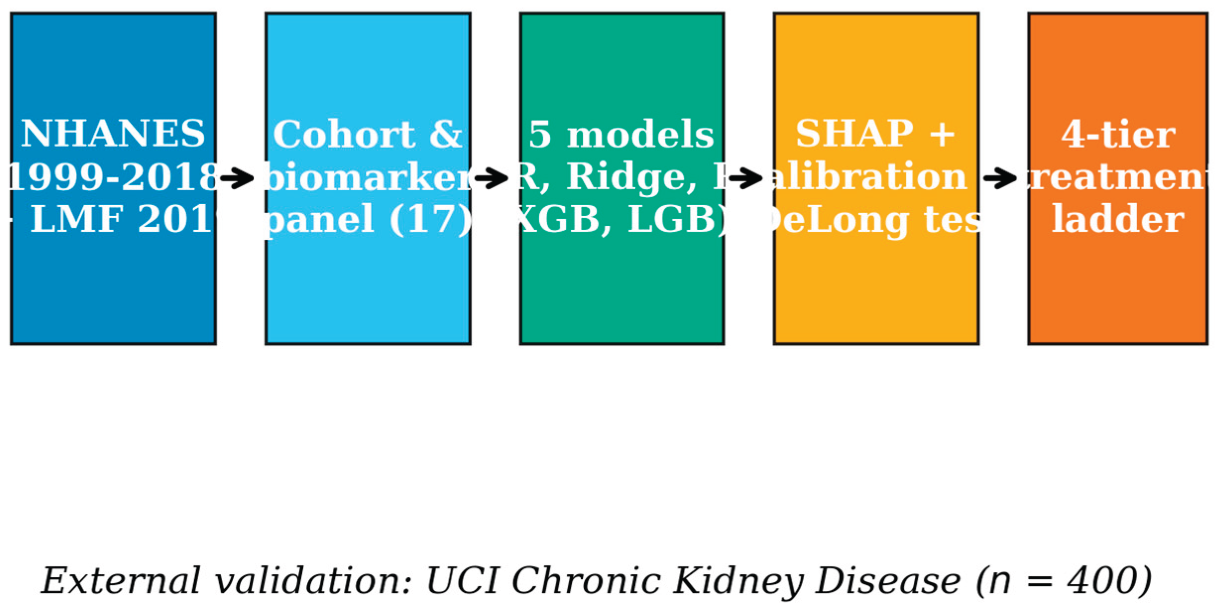
Figure 2.
Receiver-operating-characteristic curves for the five benchmarked models on the 10-year composite outcome, pooled across the held-out cross-validation folds (Table 3). Lines: LightGBM, blue solid line; Logistic regression (L2), orange dashed line; Random forest, green dash-dot line; Ridge classifier, pink dotted line; XGBoost, red dashed line. The Chance diagonal is a grey dashed reference line (AUROC = 0.500).
Figure 2.
Receiver-operating-characteristic curves for the five benchmarked models on the 10-year composite outcome, pooled across the held-out cross-validation folds (Table 3). Lines: LightGBM, blue solid line; Logistic regression (L2), orange dashed line; Random forest, green dash-dot line; Ridge classifier, pink dotted line; XGBoost, red dashed line. The Chance diagonal is a grey dashed reference line (AUROC = 0.500).
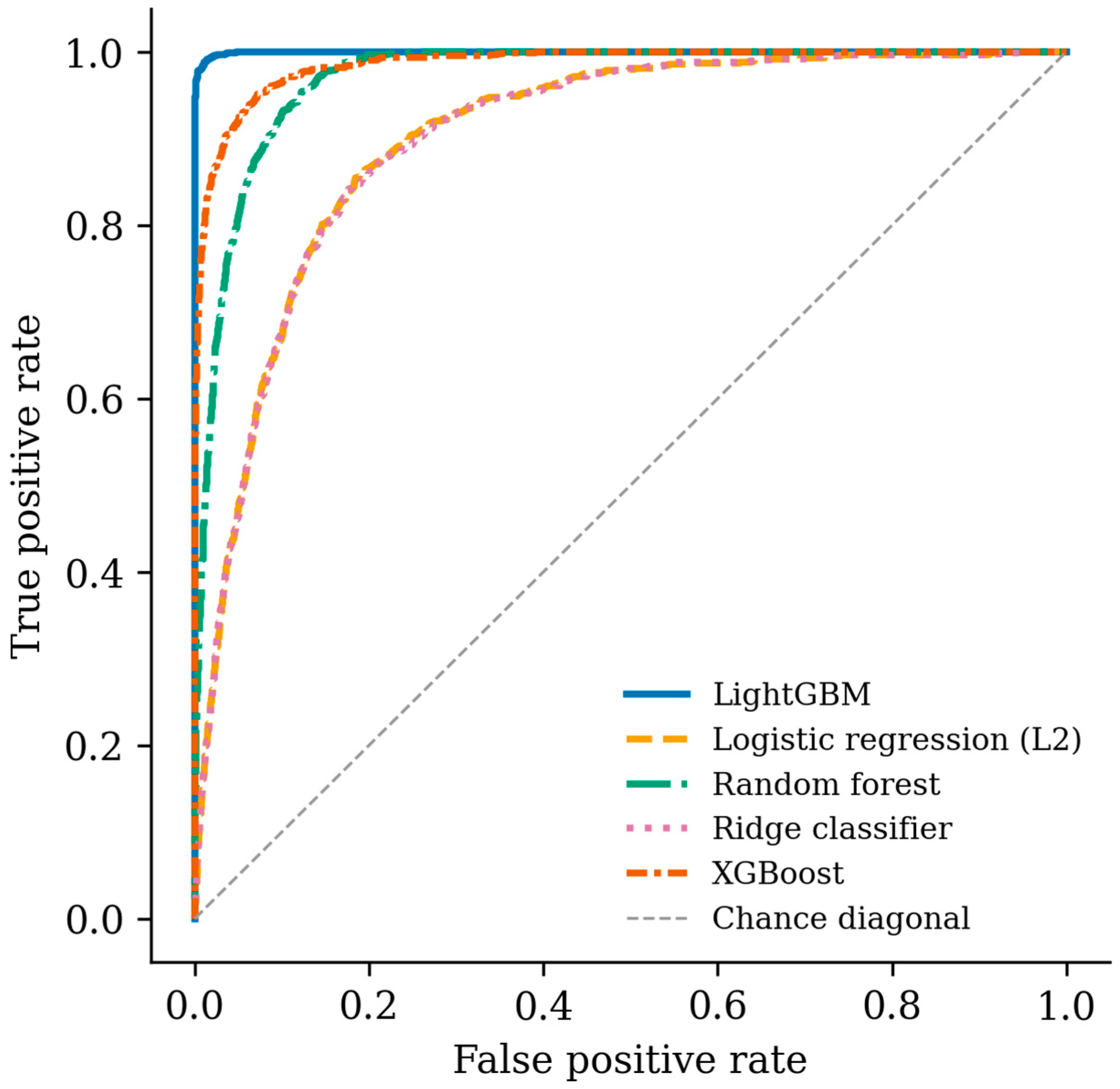
Figure 3.
Global feature importance (mean |SHAP value|) from the LightGBM TreeExplainer on the full NHANES analytic cohort (n = 24,027): horizontal bars, single blue series, top twelve features ranked top-to-bottom by descending importance (Table 4). No legend is drawn.
Figure 3.
Global feature importance (mean |SHAP value|) from the LightGBM TreeExplainer on the full NHANES analytic cohort (n = 24,027): horizontal bars, single blue series, top twelve features ranked top-to-bottom by descending importance (Table 4). No legend is drawn.
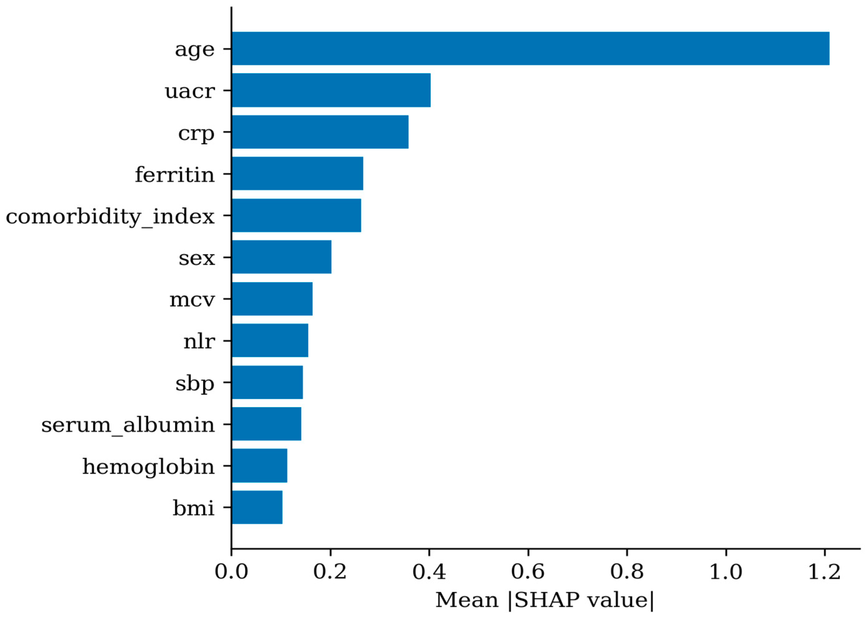
Figure 4.
Reliability diagram for the XGBoost model on pooled out-of-fold predictions. Grey dashed line: Perfect calibration. Red solid line with circular markers: Observed event rate, within each of ten equal-width predicted-probability bins over the 10-year horizon.
Figure 4.
Reliability diagram for the XGBoost model on pooled out-of-fold predictions. Grey dashed line: Perfect calibration. Red solid line with circular markers: Observed event rate, within each of ten equal-width predicted-probability bins over the 10-year horizon.
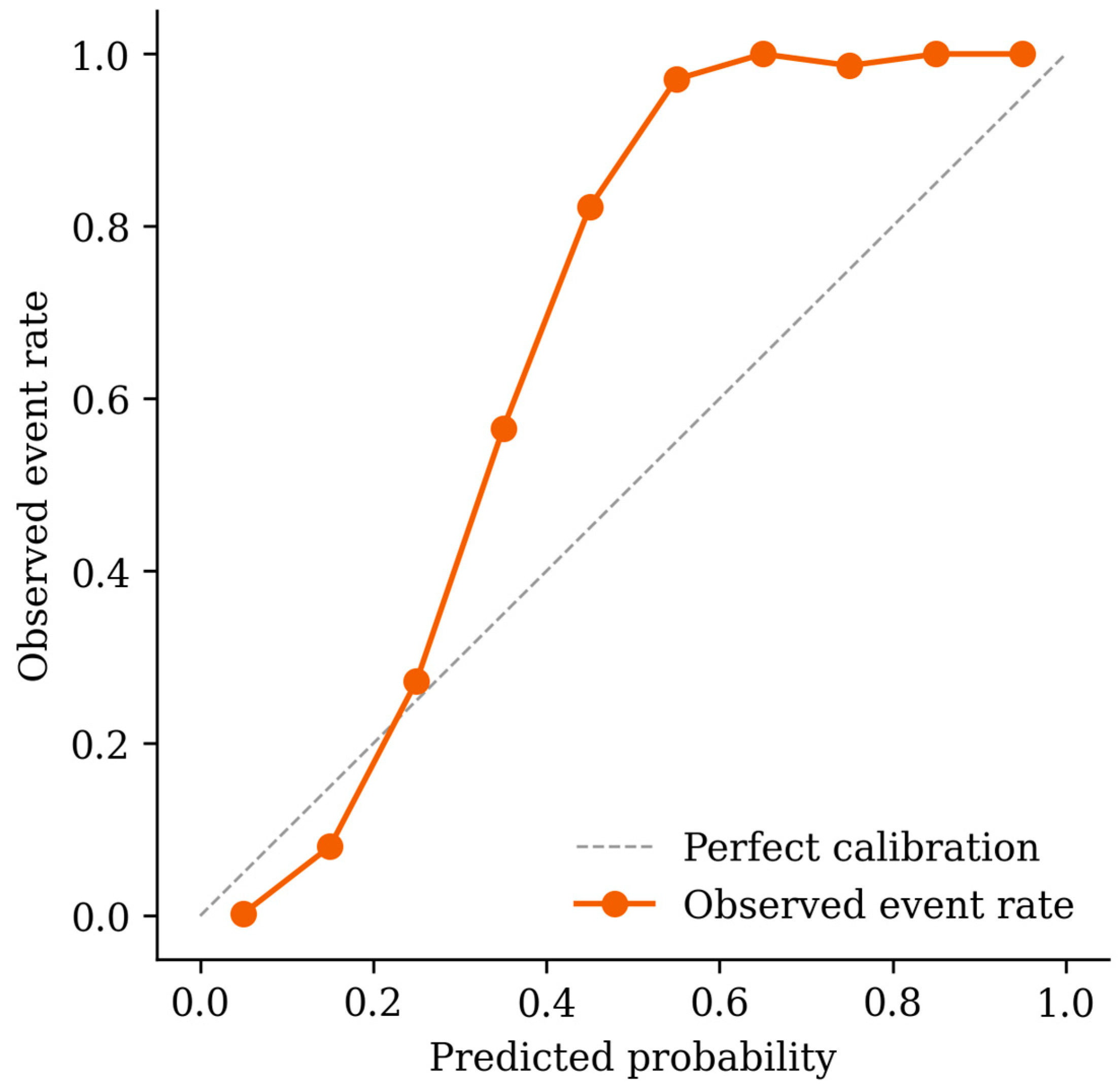
Table 1.
Inflammation–Anemia–Cardiorenal biomarker panel. NHANES variable names follow the CDC NHANES laboratory codebook conventions.
Table 1.
Inflammation–Anemia–Cardiorenal biomarker panel. NHANES variable names follow the CDC NHANES laboratory codebook conventions.
| Axis | Feature | NHANES variable | Mechanistic role |
|---|---|---|---|
| Inflammation | C-reactive protein (mg/L) | LBXCRP (1999–2010), LBXHSCRP (2015–2018) | Acute-phase reactant; elevated CRP predicts CKD progression and CV mortality [19] |
| Inflammation | Neutrophil-to-lymphocyte ratio | LBDNENO ÷ LBDLYMNO | Composite innate/adaptive immune balance; rising NLR tracks uremic inflammation [20] |
| Anemia / iron | Hemoglobin (g/dL) | LBXHGB | EPO-deficient anemia is a cardiorenal-syndrome amplifier [11,21] |
| Anemia / iron | Mean corpuscular volume (fL) | LBXMCVSI | Distinguishes iron-deficient from inflammatory anemia |
| Anemia / iron | Ferritin (ng/mL) | LBXFER | Iron stores; > 500 in CKD signals inflammation rather than overload |
| Anemia / iron | Transferrin saturation (%) | LBXIRN ÷ (LBXTIB or LBDTIB) × 100 | Iron availability for erythropoiesis |
| Nutrition / acidosis | Serum albumin (g/dL) | LBXSAL | Marker of protein–energy wasting and inflammation [22] |
| Nutrition / acidosis | Serum bicarbonate (mmol/L) | LBXSC3SI | Metabolic acidosis aggravates bone/muscle loss [23] |
| Glomerular injury | Urine albumin–creatinine ratio (mg/g) | (URXUMA × 100) ÷ URXUCR | Strongest single biomarker of glomerular injury [24] |
| Cardiorenal | Systolic blood pressure (mm Hg) | mean(BPXSY1–BPXSY4) | Hypertension is both cause and consequence of CKD |
| Cardiorenal | Diastolic blood pressure (mm Hg) | mean(BPXDI1–BPXDI4) | Same |
| Glycemic | Fasting plasma glucose (mg/dL) | LBXGLU | Diabetic-kidney-disease driver |
| Glycemic | Glycated hemoglobin (%) | LBXGH | Chronic glycemic exposure |
| Demographic | Age (years) | RIDAGEYR | Strongest single non-modifiable risk factor |
| Demographic | Sex (female) | RIAGENDR | Female sex modestly protective at equal eGFR |
| Anthropometric | Body-mass index (kg/m²) | BMXBMI | Obesity → hyperfiltration → progression |
| Comorbidity | Charlson-equivalent index | derived from MCQ, DIQ, BPQ, KIQ | Aggregate burden of diabetes, hypertension, CVD, prior MI/stroke, chronic lung disease, cancer |
A guiding constraint on the feature set was the avoidance of target leakage: none of the 17 features is mathematically derived from the outcome of interest (Section 3.4), and none was selected by an agnostic procedure that had access to the outcome.
Table 4.
Top twelve features by global mean |SHAP| (LightGBM, NHANES cohort, n = 24,027).
| Rank | Feature | Mean |SHAP| |
|---|---|---|
| 1 | Age | 1.210 |
| 2 | UACR | 0.403 |
| 3 | CRP | 0.358 |
| 4 | Ferritin | 0.267 |
| 5 | Comorbidity count | 0.262 |
| 6 | Sex | 0.203 |
| 7 | MCV | 0.165 |
| 8 | NLR | 0.155 |
| 9 | Systolic BP | 0.144 |
| 10 | Serum albumin | 0.141 |
| 11 | Hemoglobin | 0.113 |
| 12 | BMI | 0.104 |
Table 5.
Ablation study: cumulative addition of pathophysiological axes to the baseline model (XGBoost, 5-fold cross-validation). ΔAUROC computed against the immediately preceding row.
Table 5.
Ablation study: cumulative addition of pathophysiological axes to the baseline model (XGBoost, 5-fold cross-validation). ΔAUROC computed against the immediately preceding row.
| Step | Feature set added | Features (cumulative) | AUROC | ΔAUROC |
|---|---|---|---|---|
| A | Demographics + renal | 6 | 0.893 | — |
| B | + Cardiorenal (SBP, DBP) | 8 | 0.896 | +0.002 |
| C | + Glycemic (FPG, HbA1c) | 10 | 0.897 | +0.001 |
| D | + Anemia / iron | 14 | 0.905 | +0.008 |
| E | + Nutrition / acidosis | 16 | 0.906 | +0.001 |
| F | + Inflammation (CRP, NLR) | 18 | 0.912 | +0.006 |
Table 6.
Reclassification of NHANES participants against KDIGO 2024 G/A staging alone.
| Direction | n | % of 19,776 |
|---|---|---|
| Up-tiered (more-intensive therapy) | 711 | 3.6 |
| Down-tiered (less-intensive therapy) | 2810 | 14.2 |
| Concordant | 16,255 | 82.2 |
| Total reclassified | 3521 | 17.8 |
Table 7.
Transportability analysis: internal (NHANES, stratified 5-fold cross-validation) versus external (UCI Chronic Kidney Disease cohort, n = 400) AUROC for three feature sets differing in target-domain availability (Section 3.11). Δ is internal AUROC (naive) minus external AUROC.
Table 7.
Transportability analysis: internal (NHANES, stratified 5-fold cross-validation) versus external (UCI Chronic Kidney Disease cohort, n = 400) AUROC for three feature sets differing in target-domain availability (Section 3.11). Δ is internal AUROC (naive) minus external AUROC.
| Feature set | Features | Internal AUROC (naive 95 % CI) | Internal AUROC (design-aware 95 % CI) | External AUROC (95 % CI) | Δ (internal − external) |
|---|---|---|---|---|---|
| Full 17-feature panel | 17 | 0.909 (0.900–0.918) | 0.909 (0.895–0.922) | 0.598 (0.540–0.654) | 0.311 |
| Transportable 16-feature panel (transferrin saturation excluded) | 16 | 0.908 (0.898–0.916) | 0.908 (0.894–0.922) | 0.712 (0.663–0.763) | 0.196 |
| Domain-matched 6-feature panel (UCI-available features only) | 6 | 0.872 (0.861–0.882) | 0.873 (0.856–0.889) | 0.796 (0.752–0.836) | 0.077 |
Disclaimer/Publisher’s Note: The statements, opinions and data contained in all publications are solely those of the individual author(s) and contributor(s) and not of MDPI and/or the editor(s). MDPI and/or the editor(s) disclaim responsibility for any injury to people or property resulting from any ideas, methods, instructions or products referred to in the content. |
© 2026 by the authors. Licensee MDPI, Basel, Switzerland. This article is an open access article distributed under the terms and conditions of the Creative Commons Attribution (CC BY) license (http://creativecommons.org/licenses/by/4.0/).
Copyright: This open access article is published under a Creative Commons CC BY 4.0 license, which permit the free download, distribution, and reuse, provided that the author and preprint are cited in any reuse.