

Submitted:
15 August 2026
Posted:
18 August 2026
You are already at the latest version
Abstract
In strong-field ionization, complex-time saddle points govern electron ionization instant and quantum-orbit interference patterns. Neverthless, not all solutions to the saddle-point equation carry physical contributions. And saddle coalescence can also invalidate the isolated-saddle approximation. Within the strong-field-approximation framework, we propose a topology-constrained approach to reconstruct photoelectron momentum spectra. A physics-informed neural network is employed to produce candidate roots, which are subsequently refined via a Newton-type iteration. Picard–Lefschetz upward flows are adopted to pick out physically connected saddles, while local coherent continuation for pole-saddle pairs handles saddle-coalescence regions. A topological selector is defined by the non-zero support of intersection numbers to filter unphysical solutions. We test our method on hydrogen atoms subjected to six-cycle elliptically polarized laser fields and compare reconstructed spectra against direct numerical strong-field-approximation results. For 300 nm and 500 nm driving fields, the normalized relative L2 errors on the linear probability scale reach 3.793% and 3.520%, respectively.The topological selection eliminates disconnected non-physical contributions, and local continuation recovers quantum cancellation effects near saddle coalescence. Our method improves the physical interpretability of saddle-based spectrum reconstruction under strong-field approximation and is promising for other computational-physics problems involving saddle-point equations.
Keywords:
strong-field ionization
; physics-informed neural networks
; saddle-point method
; Picard–Lefschetz theory
; photoelectron momentum spectra
; coherent continuation
1. Introduction
Strong-field ionization is a fundamental process in nonlinear strong-field physics and attosecond electron dynamics. Photoelectron momentum distributions (PMDs) carry information about electron emission times, quantum-orbit interference, laser-field symmetry, and Coulomb focusing [1,2,3,4,5,6,7]. The strong-field approximation (SFA) is widely used to study PMDs. It is computationally efficient and provides a clear quantum-orbit interpretation [1,8,9,10,11]. Conventional SFA can often reproduce the main time-dependent Schrödinger equation(TDSE) spectral structures for systems with short-range binding potentials. Negative ions are typical examples. This behavior has been shown for F− ions in several laser fields. These fields include orthogonal two-color fields, short linearly polarized pulses, and counter-rotating bicircular fields [12,13,14]. The situation is different for neutral atoms. Their long-range Coulomb potential can strongly change low-energy structures and angular distributions. Coulomb-corrected SFA (CCSFA) or related trajectory corrections are therefore often needed for closer agreement with TDSE results [1,2,15,16,17,18,19]. Reconstructing PMDs through saddle-point equations (SPEs) remains an active problem in SFA and CCSFA. Such a reconstruction can provide electron emission times and quantum-orbit interference patterns [20,21,22,23,24]. Conventional local gradient-based methods and Newton-type methods require suitable initial guesses. When the laser parameters or final momentum change, the complex roots also move. The roots may approach one another, coalesce, or bifurcate. A fixed initial guess can then miss roots or produce duplicate convergence. It can also cause branch switching. Root classification creates another difficulty. A small equation residual only shows that a complex time solves the SPE. It does not show that the root contributes after a valid deformation of the original time contour. Some candidate roots are disconnected from the original contour. Others contribute little because their imaginary action is large. Accurate root finding and physical root selection are therefore separate tasks [21].
Machine learning has been applied to strong-field time-evolution and path-integral problems [25]. More recent work has used deep learning to infer molecular internuclear distances from strong-field PMDs. Transfer learning has improved these PMD inversions. Random-forest models have also characterized laser pulses from strong-field autocorrelation signals. These studies show that machine learning can extract hidden structural and dynamical information from strong-field observables [26,27,28]. Chen et al. later developed an unsupervised physics-informed neural network (PINN) for direct above-threshold-ionization SPEs [20]. This method requires neither labeled PMDs nor globally precomputed saddle roots. It directly minimizes the SPE residual. A window-based parameterization restricts different outputs to selected regions of the complex-time plane. This strategy reduces the need to choose Newton initial guesses by hand. It can generate candidate complex ionization times within a specified diagnostic region. It therefore provides a scalable candidate-root method for multibranch problems in complex laser fields. However, the PINN alone cannot reconstruct a physical PMD under a topological constraint. A small local residual does not guarantee a complete root set. Roots may be missed near coalescences and bifurcations. Branch collapse and discontinuous root counts may also occur. The PINN also lacks information about the original integration contour. It cannot determine which mathematical roots contribute to the physical amplitude. A coherent sum over all candidate roots can introduce nonphysical branches and phase interference. Independent treatment of nearby saddles can also destroy their original cancellation. Thus, we use the PINN only to generate candidate roots. The physical saddle selection requires additional topological information. In a complete Picard–Lefschetz decomposition, the intersection number determines whether a saddle contributes [2,21,29]. It describes the intersection between the original contour and the upward flow. Here, we use the condition for strict topological selection. This condition defines the binary support . It does not define a complete Picard–Lefschetz amplitude decomposition. In particular, it does not include the manifold orientation, signed intersection numbers, or all Maslov and square-root phases. Nearby saddles require collective treatment, as shown by studies of uniform approximations and Stokes smoothing [22,29,30]. We therefore preserve the coherent sum of a pole–saddle pair in local coalescence regions. This step prevents the topological selection from destroying the pair cancellation. We call this step local pole–saddle-pair coherent continuation. It is not the standard Chester–Friedman–Ursell (CFU) uniform approximation. It is also not an Airy-function uniform approximation [22,30].
In this work, we combine these steps in the PINN root-finding framework of Chen et al. The PINN first generates candidate complex roots. A Newton-type method refines the roots at each sampled momentum point. Picard–Lefschetz upward flows then select the connected saddles. Local coherent continuation treats the relevant pole–saddle pairs in coalescence regions. We test the method for hydrogen in six-cycle elliptically polarized fields at 300 and 500 nm. At each wavelength, we compare the reconstruction with direct numerical SFA time integration. Both calculations use the same Cartesian square momentum region. The comparison tests candidate-root generation, topological selection, and local coherent continuation. The present study concerns reconstruction accuracy within a common SFA framework. It does not prove that the root set is globally complete. It also does not establish agreement with TDSE results.
2. Theory and Methods
2.1. SFA Amplitude and Saddle-Point Equation
Atomic units are used throughout unless stated otherwise. For a final canonical momentum , the direct SFA amplitude in the length gauge is written as [1]
Here, is the original real-time integration contour. The dipole–field factor is . The hydrogen -state dipole transition matrix element is . The electric field is . In both numerical methods, the action is accumulated from the beginning of the pulse to the complex time t:
The laser pulse extends from to . We define the phase variable as . The major axis is along y, the helicity is positive, and the carrier phase is . The PINN and direct SFA calculations use the same vector potential:
Here, is the number of optical cycles. The angular frequency is , and the ellipticity is . The vectors and are unit vectors along the two momentum axes. The peak intensity is at both wavelengths. We use , , and .
The complex ionization times, or saddle points, satisfy
Here, is the ionization potential of hydrogen and is a complex ionization time.
The direct numerical benchmark retains the full dipole–field factor in Equation (1) and integrates along the real-time contour. The saddle-point reconstruction instead uses the pole-corrected expression for the hydrogen state employed in the present calculations [1]:
Here, and . We define and . The total ionization amplitude and the strong-field ionization probability can be given by
and
2.2. PINN Candidate-Root Generation and Newton-Type Refinement
The PINN maps normalized momentum coordinates to candidate complex-time roots. The saddle-point-equation residual constrains the candidate branches [20]. The PINN outputs serve only as initial guesses for the Newton-type method. This method refines the saddles to a residual tolerance of . Solutions within a complex-time distance of are merged as duplicates. Boundary winding numbers and global-search fallbacks provide independent root-count diagnostics. Thus, unrefined neural-network outputs are not used as physical saddle points in the final spectrum.
The candidate-root catalogs at 300 and 500 nm come from different PINN training histories. We therefore do not treat the two training protocols as identical. The later processing starts from the saved candidate-root tables. Both wavelengths use the same full-grid upward-flow parameters. They also use the same selector and the same local pole–saddle-pair continuation criteria.
The complete workflow is shown in Figure 1. The PINN generates candidate roots. A Newton-type method then refines the saddle points. Direct Picard–Lefschetz upward flows test every candidate root on the full Cartesian square momentum grid. The connected roots are coherently summed. Local pole–saddle-pair coherent continuation is applied in the identified coalescence regions.
2.3. Picard–Lefschetz Topological Selection
Let . The upward-flow trajectories from a saddle are computed in the complex-time plane by integrating the normalized one-dimensional equation
Here, the local upward direction is . The two trajectories start from . If a trajectory crosses the original real-time interval, its crossing direction determines . We integrate the upward flows with an eighth-order explicit Runge–Kutta method. Its step size adapts to the local error. The maximum arclength is 40, and the maximum step size is 0.04. The relative and absolute tolerances are and , respectively.
If a trajectory reaches the maximum arclength or the integration fails, we retry it. The retry uses an arclength of 80 and a step size of 0.02. Its relative and absolute tolerances are and , respectively. Unresolved trajectories do not enter the final topological selection.
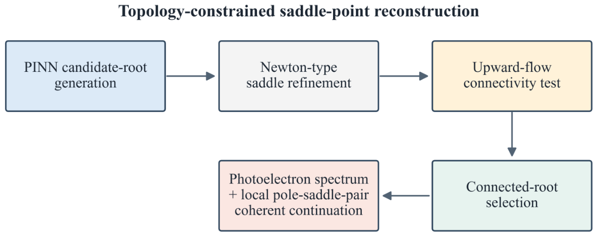
Figure 1.
Topology-constrained saddle-point reconstruction of strong-field photoelectron momentum spectra. The PINN generates candidate roots. A Newton-type method then refines the saddle points. Direct Picard–Lefschetz upward flows test every candidate root on the full Cartesian square momentum grid. The connected roots are coherently summed. Local pole–saddle-pair coherent continuation is applied in the identified coalescence regions.
Figure 1.
Topology-constrained saddle-point reconstruction of strong-field photoelectron momentum spectra. The PINN generates candidate roots. A Newton-type method then refines the saddle points. Direct Picard–Lefschetz upward flows test every candidate root on the full Cartesian square momentum grid. The connected roots are coherently summed. Local pole–saddle-pair coherent continuation is applied in the identified coalescence regions.
In the present PMD reconstruction, the intersection number is used as a hard topological connectivity criterion. At both wavelengths, direct upward flow is computed for every saved candidate-root record at all 58,081 momentum points. We define
and
According to Equation (10), the upward flow tests the connection of each saddle to the original contour. A connected saddle is retained. A disconnected saddle is removed. For a retained saddle, the program keeps its existing complex amplitude. It does not multiply this amplitude by the sign of .
Picard–Lefschetz selection does not use a fixed root index. At each momentum point, the upward flow tests each saddle separately. This avoids the limitations of root-index classification in earlier numerical saddle-point calculations [12,13,14]. Numerical sorting may cause a root label to appear or disappear. Such a label change alone does not change the physical contribution.
2.4. Local Pole–Saddle-Pair Coherent Continuation
In some local regions, two distinct saddles at the same momentum have small and . This occurs, for example, along parts of . The two contributions in Equation (5) may then cancel. Separate application of and can destroy this cancellation. We therefore define the coherent pair amplitude as
Here, . A candidate pair must satisfy and . Candidate pairs are constructed independently at each momentum point. The procedure does not track saddle branches across the full momentum space.
The final local pole–saddle-pair coherent continuation is
Let . The transition weight used in Equation (12) is
This continuation is designed for the hydrogen -state pole prefactor used here. It is not the standard Chester–Friedman–Ursell (CFU) uniform approximation derived from a canonical integral. It is also not an Airy-function uniform approximation [22,30].
2.5. Numerical Implementation and Benchmarks
The photoelectron spectra at both wavelengths are restricted to a Cartesian square grid. The complex-root search domain is and . PINN training is performed in double precision using PyTorch on a GPU. Newton-type saddle refinement, complex-action quadrature, full-grid direct upward-flow integration, and the final coherent summation are performed on the CPU. The same flow parameters and reliability criteria are used at both wavelengths. The direct numerical SFA benchmark uses the laser field in Equation (3). It also uses the hydrogen -state dipole transition matrix element.
For a quantitative comparison, each spectrum is divided by its own maximum. We denote the reconstructed spectrum by . The direct numerical SFA spectrum is denoted by . We use the normalized relative error on the linear probability scale [31]:
where i runs over all momentum-grid points. This metric directly compares the normalized photoelectron probabilities and is therefore a linear-scale metric. A value of closer to zero indicates closer agreement between the two spectra. To compare the distributions of strong and weak regions in the two spectra, we define
Here, and are the averages of and over all momentum-grid points. The quantity is the Pearson correlation coefficient [32]. A value closer to one means that the two spectra have more similar bright and dark structures.
3. Results and Discussion
3.1. Benchmarks at Two Wavelengths
Figure 2 shows the two-dimensional PMDs in the 300-nm field. Figure 2(a) gives the direct numerical SFA result. The spectrum contains a series of nearly concentric rings. A vertically elongated low-probability region appears at the center. Several narrow minima are also visible along . Figure 2(b) uses all PINN candidate roots after Newton-type refinement. By comparing panels (a) and (b), we find that most ring positions are reproduced. Their overall curvature is also reproduced. The main differences occur near . Narrow vertical discontinuities interrupt the smooth rings. Local bright and dark spots also appear in the upper and lower outer regions. Figure 2(c) shows the result after strict Picard–Lefschetz selection. The ring contours remain visible. On the logarithmic scale, the bright and dark structures are closer to those in panel (a). However, the broad annular bands away from the axis are too weak. Figure 2(d) includes local pole–saddle-pair coherent continuation. It recovers the broad bright annulus and the relative intensities of the inner and outer rings. The axis irregularities are also reduced. Thus, panel (d) is visually closest to the direct result in panel (a).
The quantitative measures support this visual comparison. Strict upward-flow classification covers 671,049 candidate-root records. The selector retains 547,200 contributions. No record is unreliable, and no retry is required. For Figure 2(b), the normalized relative error is 0.09240. The Pearson correlation coefficient is 0.97580. After strict topological selection, the Pearson correlation coefficient increases to 0.99230. This increase shows that the logarithmic bright–dark pattern is closer to the direct result. However, the error increases to 0.88353. This increase shows that the linear intensities of the broad rings are still different. The root-by-root selection removes disconnected contributions. It also changes the cancellation of near-coalescing saddle pairs in these local regions. We therefore apply local pole–saddle-pair coherent continuation. It acts on 2,145 saddle pairs at 500 grid points. The final error is 0.03793. The Pearson correlation coefficient is 0.999157.
Figure 3 shows the corresponding results in the 500-nm field. Figure 3(a) gives the direct numerical result. Its rings are more closely spaced than those at 300 nm. The central low-probability region is again elongated along the vertical direction. Several narrow minima appear along . Figure 3(b) uses all PINN/Newton roots. It preserves part of the ring pattern. However, its intensity distribution differs strongly from the direct result. The broad bright bands at central and intermediate momenta are too weak. Bright patches also appear near the upper and lower boundaries around . These patches interrupt several outer rings. Figure 3(c) gives the result after strict Picard–Lefschetz selection. The large boundary enhancements disappear. The broad annular intensity and the main ring contours are restored. A few local irregularities remain on the vertical axis. Figure 3(d) mainly changes these narrow axis regions. Away from the axis, panels (c) and (d) are almost identical. Thus, panel (d) keeps the overall improvement from topological selection and further reduces the axis artifacts.
The numerical measures again support the visual comparison. Strict upward-flow classification covers all 58,081 momentum points and 733,361 candidate-root records. The selector retains 578,590 contributions. No flow is unreliable, and no retry is required. For Figure 3(b), the error is 0.94425. The Pearson correlation coefficient is 0.94544. Strict topological selection reduces the error to 0.05112. It also raises the Pearson correlation coefficient to 0.998782. Thus, the main improvement at 500 nm comes from removing disconnected roots. The local continuation then acts on 1,174 saddle pairs at 349 grid points. The final error is 0.03520. The Pearson correlation coefficient is 0.998848.
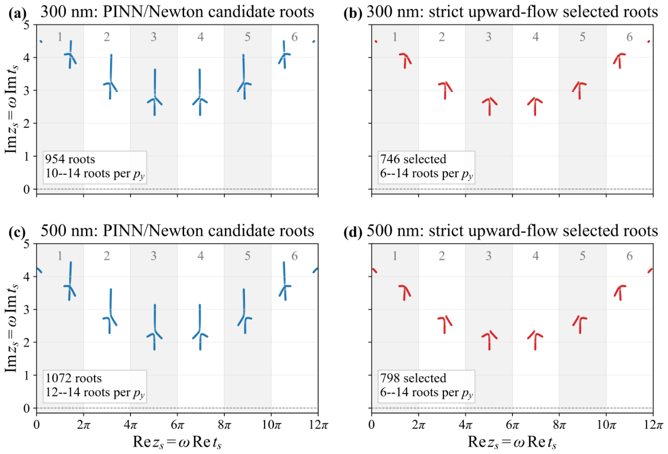
Figure 4 shows the Newton-refined roots along . Figure 4(a) gives the 300-nm results. The roots form six groups, one in each optical cycle. These groups form nearly mirror-symmetric pairs about the pulse center.The third and fourth groups are closest to the real-time axis. The first and sixth groups have larger . Several groups contain a compact fork-like pattern. A longer and nearly vertical trace extends above each of these patterns. Figure 4(b) shows the result after upward-flow selection. The lower fork-like patterns remain. Most of the upper vertical traces disappear. The total number of roots decreases from 954 to 746. At one sampled , the root number changes from 10–14 to 6–14. Some isolated roots with large remain near and . This demonstrates that the present selection scheme does not implement a simple hard cutoff on
Figure 4(c) and Figure 4(d) show the same comparison at 500 nm. The root groups in panel (c) lie closer to the real-time axis than those in panel (a). For example, the minimum in the third and fourth cycles is about 2.25 at 300 nm. It decreases to about 1.78 at 500 nm. The upward-flow selection again removes many roots from the upper traces. It does not move the retained roots. The total number decreases from 1,072 to 798. At one sampled , the root number changes from 12–14 to 6–14. Panels (b) and (d) are subsets of panels (a) and (c), respectively. Every omitted root has . Every retained root has . Therefore, the changes from panel (b) to panel (c) in Figure 2 and Figure 3 come from the connectivity test. They do not come from further root refinement. The scan only covers and a.u. It cannot establish continuous root identities or root-pair relations over the full momentum plane.
3.2. What the Topological Constraint Changes
Figure 2 and Figure 3 show the spectral changes at each stage. Figure 4 shows the corresponding reduction in the root set. Together, these results separate three numerical effects. The PINN and Newton-type method locate the saddle points. The Picard–Lefschetz selector removes saddles that are disconnected from the original contour. The local continuation restores cancellation between selected hydrogen -state terms. These operations have different roles. A smaller root residual cannot correct a wrong contour selection. A probability threshold cannot restore cancellation between two complex amplitudes.
The two wavelengths show different behavior. At 500 nm, strict topological selection provides the main improvement over the all-roots spectrum. At 300 nm, it improves the logarithmic pattern but increases the linear-scale error. The error decreases only after the pair coherence is restored. Thus, topological selection and local continuation are not interchangeable image corrections. The continuation is not applied to isolated candidate pairs.
3.3. Relation to Previous Work and Limitations
The present method builds on three established ideas. Saddle-point analysis provides a quantum-orbit interpretation of ATI photoelectron spectra [1]. Uniform asymptotic methods and Stokes smoothing can remove discontinuities or divergences near changes in saddle relevance [22,29,30]. PINNs can solve strong-field saddle-point equations without supervised root labels [20]. The present work combines these ideas in one reconstruction method. The neural network is not a PMD regressor. The topological selection is not a root-index classifier. The root distributions in Figure 4 therefore provide evidence for the reconstruction method. They are not only a schematic illustration.
The present evidence has four limitations. First, the benchmark is a reduced SFA model rather than the TDSE. Second, the upward flow is one-dimensional in complex time. It is not a general solution of the higher-dimensional thimble problem [21]. Third, strict selection uses only the nonzero support . A complete oriented reconstruction with signed needs more information. It requires continuous transport of the thimble orientation and the square-root and Maslov phases. Fourth, the local pole–saddle-pair continuation is a local amplitude continuation. It is not the standard Chester–Friedman–Ursell (CFU) uniform approximation. It is also not an Airy-function uniform approximation [22,30].
4. Conclusions
In conclusion, we have developed a topology-constrained method for reconstructing strong-field photoelectron momentum spectra. The method separates three tasks in saddle-point calculations. The first task is to find the complex-time saddle points. The second task is to test their connection to the original contour. The third task is to preserve the coherent contribution near pole–saddle-pair coalescence. A PINN generates candidate roots. A Newton-type method refines them. Independent one-dimensional Picard–Lefschetz upward flows determine . The nonzero support of defines the selector . Local pole–saddle-pair continuation preserves the cancellation of the hydrogen -state terms. It does not change the saddle-point equation or clip the final probability. At 300 nm, the final normalized relative error is . At 500 nm, it is . The corresponding Pearson correlation coefficients are and . The two wavelengths show different changes at each stage. At 500 nm, strict topological selection provides the main improvement. At 300 nm, local continuation is also needed after the root-by-root selection. It restores the cancellation. These conclusions apply to the SFA benchmark. They also apply only to the selector based on the nonzero support of . Within this scope, the method lies between direct numerical integration and an unclassified sum over all complex roots.
Author Contributions
Conceptualization, J.-H.C.; methodology, J.-H.C.; software, J.-H.C. and R.-X.N.; data curation, J.-H.C. and R.-X.N.; writing—original draft preparation, J.-H.C.; writing—review and editing, J.-H.C. All authors have read and agreed to the published version of the manuscript.
Funding
This work is supported by the National Natural Science Foundation of China (Grant No. 12064023) and the Discipline Construction Project of Lanzhou City University.
Institutional Review Board Statement
Not applicable.
Informed Consent Statement
Not applicable.
Data Availability Statement
The data supporting the findings of this study are available from the corresponding author upon reasonable request.
Conflicts of Interest
The authors declare no conflicts of interest.
Abbreviations
The following abbreviations are used in this manuscript:
| ATI | Above-threshold ionization |
| CCSFA | Coulomb-corrected strong-field approximation |
| CFU | Chester–Friedman–Ursell |
| PINN | Physics-informed neural network |
| PL | Picard–Lefschetz |
| PMD | Photoelectron momentum distribution |
| SFA | Strong-field approximation |
| SPE | Saddle-point equation |
| TDSE | Time-dependent Schrödinger equation |
References
- Milošević, D.B.; Paulus, G.G.; Bauer, D.; Becker, W. Above-threshold ionization by few-cycle pulses. J. Phys. B 2006, 39, R203–R262. [Google Scholar] [CrossRef]
- Pisanty, E.; Ivanov, M. Slalom in complex time: Emergence of low-energy structures in tunnel ionization via complex-time contours. Phys. Rev. A 2016, 93, 043408. [Google Scholar] [CrossRef]
- Dar, D.F.; Fritzsche, S. Nonlinear interference and electron dynamics: Probing photoelectron momentum distributions in strong-field ionization. Phys. Rev. A 2024, 109, L041101. [Google Scholar] [CrossRef]
- Wang, T.; Dube, Z.; Mi, Y.; Vampa, G.; Villeneuve, D.M.; Corkum, P.B.; Liu, X.; Staudte, A. Disentangling interferences in the photoelectron momentum distribution from strong-field ionization. Phys. Rev. A 2022, 106, 013106. [Google Scholar] [CrossRef]
- Douguet, N.; Bartschat, K. Photoelectron momentum distributions in the strong-field ionization of atomic hydrogen by few-cycle elliptically polarized optical pulses. Phys. Rev. A 2022, 106, 053112. [Google Scholar] [CrossRef]
- Xu, R.H.; Zhao, Y.K.; Chen, Y.J.; Fu, L.B. Coulomb-induced asymmetry on photoelectron momentum distributions in orthogonal two-color laser fields. Phys. Rev. A 2021, 103, 023109. [Google Scholar] [CrossRef]
- Werby, N.; Natan, A.; Forbes, R.; Bucksbaum, P.H. Disentangling the subcycle electron momentum spectrum in strong-field ionization. Phys. Rev. Res. 2021, 3, 023065. [Google Scholar] [CrossRef]
- Keldysh, L.V. Ionization in the Field of a Strong Electromagnetic Wave. Sov. Phys. JETP 1965, 20, 1307–1314. [Google Scholar]
- Faisal, F.H.M. Multiple absorption of laser photons by atoms. J. Phys. B 1973, 6, L89–L92. [Google Scholar] [CrossRef]
- Reiss, H.R. Effect of an intense electromagnetic field on a weakly bound system. Phys. Rev. A 1980, 22, 1786–1813. [Google Scholar] [CrossRef]
- Lewenstein, M.; Balcou, P.; Ivanov, M.Y.; L’Huillier, A.; Corkum, P.B. Theory of high-harmonic generation by low-frequency laser fields. Phys. Rev. A 1994, 49, 2117–2132. [Google Scholar] [CrossRef] [PubMed]
- Chen, J.H.; Han, M.; Xiao, X.R.; Peng, L.Y.; Liu, Y. Atomic-orbital-dependent photoelectron momentum distributions for F- ions by orthogonal two-color laser fields. Phys. Rev. A 2018, 98, 033403. [Google Scholar] [CrossRef]
- Chen, J.H.; Xiao, X.R.; Zhao, S.F.; Peng, L.Y. Dependence of direct and rescattered photoelectron spectra of fluorine anions on orbital symmetry in a short laser pulse. Phys. Rev. A 2020, 101, 033409. [Google Scholar] [CrossRef]
- Chen, J.H.; Wen, L.C.; Zhao, S.F. Orbital-resolved photoelectron momentum distributions of F- ions in a counter-rotating bicircular field. Opt. Express 2023, 31, 5708–5722. [Google Scholar] [CrossRef] [PubMed]
- Li, X.; Liu, X.; Wang, C.; Ben, S.; Zhou, S.; Yang, Y.; Song, X.; Chen, J.; Yang, W.; Ding, D. Coulomb focusing in attosecond angular streaking. Light Sci. Appl. 2024, 13, 250. [Google Scholar] [CrossRef] [PubMed]
- Lv, Q.; Klaiber, M.; He, P.L.; Hatsagortsyan, K.Z.; Keitel, C.H. Photoelectron low-energy structures for arbitrary ellipticity of a strong laser field. Commun. Phys. 2025, 8, 462. [Google Scholar] [CrossRef]
- Böning, B.; Fritzsche, S. Partial-wave representation of the strong-field approximation. II. Coulomb asymmetry in the photoelectron angular distribution of many-electron atoms. Phys. Rev. A 2023, 107, 023108. [Google Scholar] [CrossRef]
- Rook, T.; Habibović, D.; Rodriguez, L.C.; Milošević, D.B.; Faria, C.F.d.M. Impact of the continuum Coulomb interaction in quantum-orbit-based treatments of high-order above-threshold ionization. Phys. Rev. A 2024, 109, 033115. [Google Scholar] [CrossRef]
- Chen, Z.Y.; Shen, S.Q.; Li, Y.P.; Yang, Z.Q.; Che, J.Y.; Chen, Y.J. Coulomb-related symmetry in laser-induced tunneling ionization of atoms and molecules. Phys. Rev. A 2025, 111, 053118. [Google Scholar] [CrossRef]
- Chen, J.; Hashim, S.; Figueira de Morisson Faria, C. Physics-informed neural networks for solving saddle-point equations in strong-field physics with tailored fields. Phys. Rev. Res. 2026, 8, 033029. [Google Scholar] [CrossRef]
- Weber, A.; Feldbrugge, J.; Pisanty, E. Universal approach to saddle-point methods in attosecond science. Phys. Rev. A 2026, 113, 063111. [Google Scholar] [CrossRef]
- Milošević, D.B. Application of the uniform approximation to integrals occurring in ionization by a strong elliptically polarized laser field. Phys. Rev. A 2025, 111, 053105. [Google Scholar] [CrossRef]
- Habibović, D.; Milošević, D.B. Complete classification and additional saddle-point solutions for high-order above-threshold ionization induced by a strong laser field. Phys. Rev. A 2025, 111, 023103. [Google Scholar] [CrossRef]
- Rook, T.; Habibović, D.; Faria, C.F.d.M. Energy-conservation conditions in the saddle-point approximation for the strong-field ionization of atoms. Phys. Rev. A 2025, 111, 023107. [Google Scholar] [CrossRef]
- Liu, X.; Zhang, G.; Li, J.; Shi, G.; Zhou, M.; Huang, B.; Tang, Y.; Song, X.; Yang, W. Deep Learning for Feynman’s Path Integral in Strong-Field Time-Dependent Dynamics. Phys. Rev. Lett. 2020, 124, 113202. [Google Scholar] [CrossRef] [PubMed]
- Shvetsov-Shilovski, N.I.; Lein, M. Deep learning for retrieval of the internuclear distance in a molecule from interference patterns in photoelectron momentum distributions. Phys. Rev. A 2022, 105, L021102. [Google Scholar] [CrossRef]
- Shvetsov-Shilovski, N.I.; Lein, M. Transfer learning, alternative approaches, and visualization of a convolutional neural network for retrieval of the internuclear distance in a molecule from photoelectron momentum distributions. Phys. Rev. A 2023, 107, 033106. [Google Scholar] [CrossRef]
- Kolbasova, D.; Santra, R. Laser-pulse characterization using strong-field autocorrelation patterns and random-forest-based machine learning. Phys. Rev. A 2023, 107, 013520. [Google Scholar] [CrossRef]
- Berry, M.V. Uniform asymptotic smoothing of Stokes’s discontinuities. Proc. R. Soc. Lond. A 1989, 422, 7–21. [Google Scholar] [CrossRef]
- Figueira de Morisson Faria, C.; Schomerus, H.; Becker, W. High-order above-threshold ionization: The uniform approximation and the effect of the binding potential. Phys. Rev. A 2002, 66, 043413. [Google Scholar] [CrossRef]
- Raissi, M.; Perdikaris, P.; Karniadakis, G.E. Physics-informed neural networks: A deep learning framework for solving forward and inverse problems involving nonlinear partial differential equations. J. Comput. Phys. 2019, 378, 686–707. [Google Scholar] [CrossRef]
- Rodgers, J.L.; Nicewander, W.A. Thirteen Ways to Look at the Correlation Coefficient. Am. Stat. 1988, 42, 59–66. [Google Scholar] [CrossRef]
Figure 2.
Photoelectron momentum spectra on the full Cartesian square grid at 300 nm. Panel (a) shows direct numerical SFA integration. Panel (b) uses all PINN candidate roots after Newton-type refinement. Panel (c) uses the strict selector . Panel (d) adds local pole–saddle-pair coherent continuation. This continuation acts on 2,145 saddle pairs at 500 grid points. It reduces the normalized relative error from 0.88353 to 0.03793. Each spectrum is normalized by its own maximum. All panels use the range –1 and the same square grid.
Figure 2.
Photoelectron momentum spectra on the full Cartesian square grid at 300 nm. Panel (a) shows direct numerical SFA integration. Panel (b) uses all PINN candidate roots after Newton-type refinement. Panel (c) uses the strict selector . Panel (d) adds local pole–saddle-pair coherent continuation. This continuation acts on 2,145 saddle pairs at 500 grid points. It reduces the normalized relative error from 0.88353 to 0.03793. Each spectrum is normalized by its own maximum. All panels use the range –1 and the same square grid.
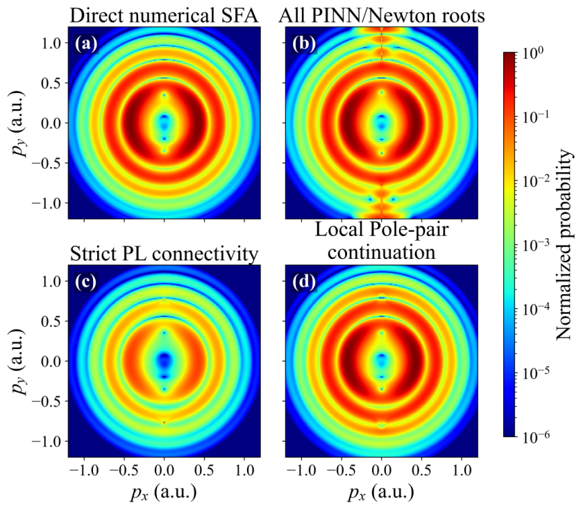
Figure 3.
Photoelectron momentum spectra on the full Cartesian square grid at 500 nm. Panel (a) shows direct numerical SFA integration. Panel (b) uses all PINN candidate roots after Newton-type refinement. Panel (c) uses the strict selector . Panel (d) adds local pole–saddle-pair coherent continuation. This continuation acts on 1,174 saddle pairs at 349 grid points. It reduces the normalized relative error from 0.05112 to 0.03520. Each spectrum is normalized by its own maximum. All panels use the range –1 and the same square grid.
Figure 3.
Photoelectron momentum spectra on the full Cartesian square grid at 500 nm. Panel (a) shows direct numerical SFA integration. Panel (b) uses all PINN candidate roots after Newton-type refinement. Panel (c) uses the strict selector . Panel (d) adds local pole–saddle-pair coherent continuation. This continuation acts on 1,174 saddle pairs at 349 grid points. It reduces the normalized relative error from 0.05112 to 0.03520. Each spectrum is normalized by its own maximum. All panels use the range –1 and the same square grid.
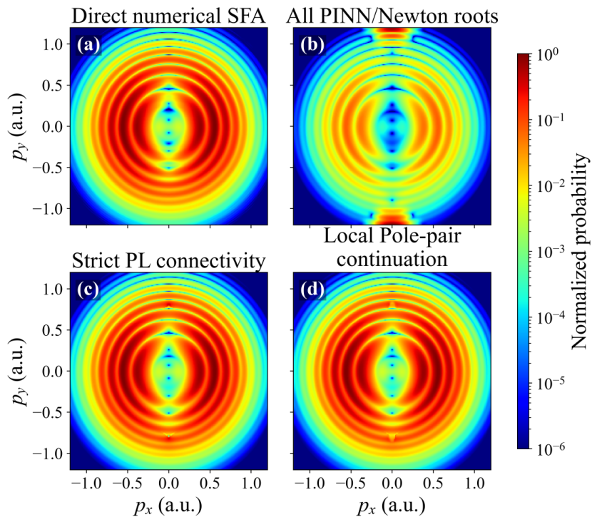
Figure 4.
Axis scans of saddle roots at and a.u. The horizontal axis is . The vertical axis is . Panels (a) and (c) show all Newton-refined roots at 300 and 500 nm. Panels (b) and (d) show the roots retained by the upward-flow selection. At 300 nm, each sampled has 10–14 candidate roots and 6–14 selected roots. At 500 nm, it has 12–14 candidate roots and 6–14 selected roots. Each point is one Newton-refined saddle root at one sampled momentum; vertical bands mark optical cycles.
Figure 4.
Axis scans of saddle roots at and a.u. The horizontal axis is . The vertical axis is . Panels (a) and (c) show all Newton-refined roots at 300 and 500 nm. Panels (b) and (d) show the roots retained by the upward-flow selection. At 300 nm, each sampled has 10–14 candidate roots and 6–14 selected roots. At 500 nm, it has 12–14 candidate roots and 6–14 selected roots. Each point is one Newton-refined saddle root at one sampled momentum; vertical bands mark optical cycles.
Disclaimer/Publisher’s Note: The statements, opinions and data contained in all publications are solely those of the individual author(s) and contributor(s) and not of MDPI and/or the editor(s). MDPI and/or the editor(s) disclaim responsibility for any injury to people or property resulting from any ideas, methods, instructions or products referred to in the content. |
© 2026 by the authors. Licensee MDPI, Basel, Switzerland. This article is an open access article distributed under the terms and conditions of the Creative Commons Attribution (CC BY) license (http://creativecommons.org/licenses/by/4.0/).
Copyright: This open access article is published under a Creative Commons CC BY 4.0 license, which permit the free download, distribution, and reuse, provided that the author and preprint are cited in any reuse.