

Submitted:
14 August 2026
Posted:
17 August 2026
You are already at the latest version
Abstract
River–lake confluence zones are shaped by inflow hydrology, evaporative concentration, and water mixing, providing natural systems for examining phytoplankton responses to environmental gradients. Here, we investigated Siling Co and adjacent river–lake confluence zones at elevations above 4,500 m. We integrated genus-level phytoplankton cell-density and biomass data with 22 environmental variables from 14 sampling events at 10 sites, including seven Lake and seven River samples. Community diversity, composition, and community–environment associations were evaluated using ordination, permutation tests, correlation analyses, distance-based redundancy analysis, Mantel tests, and multi-method evidence integration. In total, 54 genera were recorded, with Bacillariophyta representing the dominant phylum. Lake and River samples overlapped in community composition, whereas sampling period explained more genus-level variation than water-body type. Major-ion and mineralization gradients were consistently associated with community turnover. pH and SiO₂ were associated with cell-density composition, whereas Cl⁻ was associated with biomass composition. Cyanobacterial relative biomass was positively correlated with total nitrogen and negatively correlated with SO₄²⁻. These findings indicate that phytoplankton community structure in the Siling Co river–lake confluence zone cannot be attributed simply to two discrete habitat types, namely lakes and rivers, and provide a new perspective on community assembly in extremely high-altitude river–lake confluence zones.
Keywords:
plateau lakes
; river–lake confluence zones
; phytoplankton
; ionic composition
; mineralization
; distance-based redundancy analysis (db-RDA)
1. Introduction
Phytoplankton are key components of primary production, material cycling, and energy transfer through aquatic food webs. Their community composition, abundance, and diversity often respond rapidly to changes in water temperature, light availability, nutrient concentrations, hydrodynamic conditions, and water chemistry. They therefore serve both as indicators of ecosystem status and as sensitive biological signals of environmental filtering processes [1,2].
River–lake confluence zones formed where rivers enter lakes are not simply juxtaposed riverine and lacustrine water bodies. Within a limited spatial extent, runoff inputs, evaporative concentration, ion exchange, water mixing, and variation in water residence time can collectively generate continuous gradients in salinity, dissolved substances, nutrients, and suspended particulate matter. Hydrodynamic processes can also alter the transport pathways and availability of inflowing water and associated nutrients within the euphotic zone [3,4]. Consequently, phytoplankton responses to such gradients are often taxon-specific, and interactions among physicochemical variables may explain community variation better than any single factor alone.
In waters with relatively high salinity or mineralization, osmoregulatory costs, ionic ratios, and nutrient availability can jointly alter competitive relationships among algal groups. Recent field and experimental studies have shown that even modest changes in salinity can restructure planktonic communities, alter community assembly processes, and affect the relative dominance of groups such as cyanobacteria through responses of competitors or grazers [5,6,7,8,9,10]. In addition, cell density and biomass do not provide equivalent descriptions of community change. Small-sized or filamentous taxa may contribute high cell densities, whereas large taxa or taxa with high per-cell biomass may dominate biomass accumulation. Joint analyses of cell density, biomass, α-diversity, and genus-level composition can therefore reduce the risk of interpreting a single quantitative metric as a complete proxy for community ecological function.
The main basin of Siling Co, its littoral sites, and the confluence zones of its inflowing rivers together form a high-altitude river–lake transitional system with pronounced hydrochemical heterogeneity. Plateau lakes are highly sensitive to hydroclimatic change, salinity differentiation, and nutrient redistribution. Recent studies from the Tibetan Plateau have further linked hydroclimatic processes, gradients in conductivity or salinity, and nutrient stoichiometry to the structure and assembly of aquatic communities [11,12,13,14,15]. Available data indicate numerical differences between lake and river sites in salinity, ionic composition, nutrients, and silicate. However, owing to limited sample size and multiple-testing constraints, between-group differences for individual variables are not consistently detected. Thus, rather than focusing solely on whether lake and river sites support completely distinct communities, it is necessary to identify continuous environmental gradients spanning both site types and examine their relationships with community turnover.
Based on genus-level cell-density and biomass matrices from 14 sampling events, this study first characterized environmental conditions and the abundance, diversity, and taxonomic composition of phytoplankton communities. We then used Bray–Curtis distances, principal coordinates analysis (PCoA), non-metric multidimensional scaling (NMDS), and permutational multivariate analysis of variance (PERMANOVA) to assess community differences associated with water-body type and sampling period. Spearman correlation, distance-based redundancy analysis (db-RDA), Mantel tests, and partial Mantel tests were further combined to identify environmental associations at the levels of individual variables, constrained ordination, and distance matrices. Finally, candidate drivers were evaluated according to convergent evidence from multiple analytical approaches. This framework was designed to distinguish relatively robust environment–community associations from exploratory signals and to provide a reproducible analytical pathway for phytoplankton monitoring in high-altitude river–lake confluence zones.
2. Materials and Methods
2.1. Study Area and Sampling Design
The study area comprised Siling Co and adjacent river–lake confluence zones at elevations above 4,500 m. Sampling sites encompassed the main basin and littoral areas of Siling Co, as well as confluence zones associated with the Zagya Zangbo River, Zhagen Zangbo River, Ngari Zangbo River, and Dara Zangbo River river systems. In total, 10 spatial sampling sites (S1–S10) were established, spanning 88.522939–89.530935° E and 31.519086–32.042631° N (Figure 1).
A total of 14 sampling events were included in this study, comprising seven lake samples (Lake) and seven river samples (River). Sampling was conducted in June, August, and October 2023, and in September 2024. Sites S1, S2, S3, and S5 were repeatedly sampled across sampling periods. Because months and years were not fully crossed in the sampling design, all time-related inferences are described as differences among sampling periods and are not interpreted as strictly independent seasonal or interannual effects.
2.2. Field Sampling, Environmental Measurements, and Phytoplankton Identification
Each sampling event was assigned a unique identifier (sample_uid) and linked to the corresponding sample_id, sampling-site name, geographic coordinates, water-body type, sampling year, and sampling month. Environmental data comprised 22 variables, including water temperature (WT), dissolved oxygen (DO), pH, turbidity (Tur), conductivity (CON), total dissolved solids (TDS), salinity (SAL), nitrogen and phosphorus nutrients, major ions, total hardness (TH), iron (Fe), sulfide (S2−), and silica (SiO2).
2.2.1. Sampling for Physicochemical Water-Quality Variables
Six variables, namely pH, water temperature, dissolved oxygen, total dissolved solids, conductivity, and salinity, were measured in situ using an AZ86031 multiparameter water-quality meter (Hengxin). Water samples for the remaining variables were collected from the surface layer, 10 cm below the water surface, using clean 500 mL plastic bottles. Before sampling, each bottle was rinsed with the water to be sampled. The rinse water was discarded, after which the bottle was filled with sample water while avoiding air bubbles and immediately sealed tightly. Samples were stored in a vehicle-mounted refrigerator at 4 °C and transported to the laboratory within 48 h for physicochemical analyses.

Table 1.
Physicochemical water-quality variables, units, analytical methods, and instruments.
| Physicochemical variable | Code | Unit | Analytical method | Instrument |
|---|---|---|---|---|
| pH | pH | — | In situ measurement | Hengxin AZ86031 multiparameter water-quality meter |
| Water temperature | WT | °C | In situ measurement | Hengxin AZ86031 multiparameter water-quality meter |
| Dissolved oxygen | DO | mg/L | In situ measurement | Hengxin AZ86031 multiparameter water-quality meter |
| Total dissolved solids | TDS | Ppm | In situ measurement | Hengxin AZ86031 multiparameter water-quality meter |
| Conductivity | CON | μS/cm | In situ measurement | Hengxin AZ86031 multiparameter water-quality meter |
| Salinity | SAL | Ppt | In situ measurement | Hengxin AZ86031 multiparameter water-quality meter |
| Turbidity | Tur | TU | — | Merck Prove 600 laboratory multiparameter water-quality analyzer |
| Potassium | K+ | mg/L | GB 11904-89 | Merck Prove 600 laboratory multiparameter water-quality analyzer |
| Sodium | Na+ | mg/L | GB 11904-89 | Merck Prove 600 laboratory multiparameter water-quality analyzer |
| Calcium | Ca2+ | mg/L | GB 11904-89 | Merck Prove 600 laboratory multiparameter water-quality analyzer |
| Silicon | SiO2 | mg/L | GB/13196-91 | Merck Prove 600 laboratory multiparameter water-quality analyzer |
| Iron | Fe | mg/L | MEPPRC, 2002 | Merck Prove 600 laboratory multiparameter water-quality analyzer |
| Chloride | Cl− | mg/L | HJ/T 84-2001 | Merck Prove 600 laboratory multiparameter water-quality analyzer |
| Sulfate | SO42- | mg/L | GB/13196-91 | Merck Prove 600 laboratory multiparameter water-quality analyzer |
| Sulfite | SO32- | mg/L | GB/13196-91 | Merck Prove 600 laboratory multiparameter water-quality analyzer |
| Nitrate | NO3− | mg/L | GB 7480-87 | Merck Prove 600 laboratory multiparameter water-quality analyzer |
| Nitrite | NO2− | mg/L | GB/T 8538-2008 | Merck Prove 600 laboratory multiparameter water-quality analyzer |
| Ammonium nitrogen | NH4+ | mg/L | GB 7479-87 | Merck Prove 600 laboratory multiparameter water-quality analyzer |
| Total phosphorus | TP | mg/L | GB 11894-89 | Merck Prove 600 laboratory multiparameter water-quality analyzer |
| Total nitrogen | TN | mg/L | GB 11894-89 | Merck Prove 600 laboratory multiparameter water-quality analyzer |
| Sulfide | S2− | mg/L | GB/T 16489-1996 | Merck Prove 600 laboratory multiparameter water-quality analyzer |
2.2.2. Phytoplankton Sampling and Identification
A 10 L water sample was filtered through a No. 25 plankton net with a mesh size of 0.064 mm. The resulting concentrated sample was fixed with Lugol’s solution and transported to the laboratory for analysis. Before enumeration, the concentrated sample was thoroughly homogenized, and a 0.1 mL aliquot was transferred to a counting chamber for microscopic observation at 400× magnification (10× ocular × 40× objective). Each counting chamber comprised 46 rows, of which N rows were enumerated. Each sample was counted twice, and the mean value was used. Counts were considered valid when the difference between each count and the mean was <10%; otherwise, a third count was performed. Phytoplankton were identified to the species or genus level.
To improve the comparability of sampling results, key details of the net-sampling, Lugol’s fixation, and microscopic-counting procedures are provided above. Recent methodological comparisons indicate that mesh size, sampling volume, and sampling approach can affect phytoplankton detection and the characterization of community composition. Accordingly, the present results primarily represent taxa that were efficiently retained by the 0.064 mm mesh and identified through the counting procedure used here. Comparisons across studies should therefore consider sampling volume, fixation method, and counting scale [16].
2.3. Environmental Data Quality Control and Preprocessing
For environmental characterization and between-group comparisons, missing values were first quantified and potential outliers were identified using the interquartile range method. In descriptive statistics and Mann–Whitney U tests, missing records were automatically excluded on a variable-wise basis. Given the small sample size and the skewed distributions of some variables, differences between Lake and River samples were assessed using two-sided Mann–Whitney U tests, whereas differences among sampling periods were evaluated using Kruskal–Wallis tests. All P values were adjusted for the false discovery rate (FDR) using the Benjamini–Hochberg procedure.
For correlation analyses and multivariate ordination, missing environmental values were imputed using variable medians. Non-negative variables with an absolute skewness >1 and deemed suitable for transformation were log10(x + 1)-transformed and subsequently standardized as z scores. To reduce redundancy among explanatory variables, collinearity was assessed using Spearman rank correlations and variance inflation factors (VIFs). Highly correlated variables, including pH, TDS, and CON, were not simultaneously retained in the same constrained ordination model. Candidate variables were selected by considering both statistical diagnostics and ecological relevance.
2.4. Phytoplankton Community Metrics and Taxonomic Composition
Phytoplankton communities were characterized using genus-level cell-density and biomass matrices comprising 14 samples and 54 genera. Total cell density (N) and total biomass (B) for each sample were calculated as the sums of the cell densities and biomasses, respectively, of all detected genera. Based on cell density, the Margalef richness index (d), Shannon–Wiener diversity index (H), Pielou evenness index (J), and Simpson dominance index (S) were calculated. Here, pi denotes the relative cell density of genus i in a sample, and Sr denotes the number of recorded genera: , , , .
Phylum-level composition was summarized using a genus-to-phylum taxonomic mapping table, and relative cell density and relative biomass were calculated separately. The relative contribution of phylum i was calculated as where Ai represents its cell density or biomass. Dominant phyla were identified by integrating mean relative cell density, mean relative biomass, and frequency of occurrence. Dominant taxa at the genus level were screened according to mean relative contribution, frequency of occurrence, and habitat affinity. As cell density and biomass represent numerical structure and material contribution, respectively, they were analyzed independently and cross-checked during interpretation.
2.5. Community β-Diversity, Ordination, and Permutation Tests
Genus-level abundances were first converted to within-sample relative abundances and then Hellinger-transformed to reduce the disproportionate influence of dominant genera on distance calculations and linear ordination. Bray–Curtis dissimilarities were calculated from the transformed matrices, and principal coordinates analysis (PCoA) was conducted separately for cell-density and biomass communities. Two-dimensional non-metric multidimensional scaling (NMDS) was used as a robustness check, with ordination quality evaluated using stress values. In ordination plots, colours distinguished Lake and River samples, point shapes indicated sampling periods, and 95% confidence ellipses were displayed.
PERMANOVA with 4,999 permutations was used to evaluate the contributions of water-body type (Type), sampling month (Month), sampling year (Year), the additive Type + Month model, and environmental PCA axes to variation in community composition. The proportion of explained variation was expressed as R2. PERMDISP with 999 permutations was additionally performed to test for differences in within-group dispersion. To reduce the influence of repeated sampling, relative community compositions from the same sample_id were averaged to obtain 10 independent sites, and the Type effect was retested as a sensitivity analysis. The association between cell-density and biomass Bray–Curtis distance matrices was assessed using a permutation-based distance-matrix correlation analysis.
2.6. Community–Environment Association Analyses
Spearman rank correlations were used to examine associations between environmental variables and total cell density, total biomass, α-diversity metrics, phylum-level relative abundance, and relative abundance of dominant genera. Multiple-testing correction was performed separately within five analytical families: overall community metrics, phylum-level cell density, phylum-level biomass, cell density of dominant genera, and biomass of dominant genera. Associations with |ρ| ≥ 0.60 and an FDR-adjusted P < 0.05 were defined as statistically supported strong correlations. Associations with |ρ| ≥ 0.60 and an unadjusted P < 0.05, but a non-significant FDR-adjusted P value, were defined as exploratory strong correlations. To assess robustness, key analyses were repeated using median-aggregated values for repeatedly sampled sites, yielding 10 independent sites.
2.7. Constrained Ordination and Environmental Distance-Matrix Analyses
Constrained ordination analyses used genus-level cell-density and biomass community matrices as response variables. Hellinger-transformed redundancy analysis (Hellinger-RDA), canonical correspondence analysis (CCA), and distance-based redundancy analysis (db-RDA) based on Bray–Curtis distances were compared according to gradient lengths from correspondence analysis, the proportion of zero values, and model suitability. db-RDA was selected as the primary model. Candidate environmental variables entered the final model after correlation screening, VIF assessment, and forward selection. Forward selection used 4,999 conditional permutations, whereas the final model was evaluated using 9,999 permutations. Given the limited sample size (n = 14), the number of variables in each model was strictly limited to avoid overfitting.
Mantel tests were based on Bray–Curtis distances calculated from Hellinger-transformed community matrices and Euclidean distances calculated for environmental variable groups, using Spearman correlations and 9,999 two-sided permutations. Environmental variables were grouped into six categories: all environmental variables, basic physicochemical variables, salinity/mineralization variables, nutrients, major ions, and other variables. Cell-density and biomass results were subjected to separate FDR corrections. A binary Type distance matrix was further constructed for partial Mantel tests to determine whether major-ion and mineralization signals could be attributed solely to Lake/River classification. As geographic distance was not controlled in these analyses, the results were interpreted as sensitivity evidence rather than causal tests.
2.8. Multi-Method Evidence Integration and Random Forest Support Analysis
Candidate drivers were evaluated by integrating six evidence sources: Lake/River differences in environmental variables, environmental PCA, community–environment Spearman correlations, RDA/db-RDA/CCA, Mantel tests, and random forest analysis. The predefined weights for these evidence sources were 5%, 10%, 30%, 35%, 15%, and 5%, respectively, thereby emphasizing direct evidence of community responses. Each evidence source was converted to a normalized score ranging from 0 to 1, followed by a minor completeness adjustment according to the proportion of missing values for each variable. The integrated score reflects consistency of evidence across analytical methods rather than the causal effect size of an environmental factor.
Random forest analysis was used only as an exploratory supplementary approach. Total cell density, total biomass, the Shannon index, relative cell density of dominant phyla, and relative cell density of dominant genera were used as response variables. Predictor variables were selected based on the preceding non-machine-learning evidence, and highly correlated redundant variables were excluded. Resampling was grouped by sample_id to reduce optimistic bias caused by repeated sampling. Given the limited sample size, variable importance was used only for supplementary ranking and did not replace the direct evidence provided by permutation tests and constrained ordination.
2.9. Statistical Software
Data processing, statistical analyses, and figure generation were conducted primarily in Python 3.14 using pandas, NumPy, SciPy, statsmodels, scikit-learn, Matplotlib, openpyxl, and related packages. The number of permutations used for each permutation-based test and the FDR-correction procedure are specified in the corresponding analyses.
3. Results
3.1. Environmental Gradients and Lake–River Sample Distribution
A total of 14 sampling events were included in the environmental analysis, comprising seven Lake and seven River samples. Missing values were recorded for Na+ (five values), SO32− (four values), Tur (two values), K+ (two values), and S2− (one value); all other environmental variables had complete data. In the environmental principal component analysis, PC1 and PC2 explained 27.56% and 22.80% of the environmental variation, respectively, accounting for 50.36% cumulatively (Figure 2). Strong correlations among environmental variables after FDR correction are shown in Table 2.
The largest positive loadings on PC1 were NH4+ (0.494), SiO2 (0.449), and SO32− (0.429), whereas the largest negative loadings were SAL (−0.349) and SO42− (−0.303). For PC2, Ca2+ (0.552) and TP (0.333) showed the largest positive loadings, while DO (−0.462), SO42− (−0.394), SO32− (−0.301), and SAL (−0.292) showed the largest negative loadings. The mean PC1 scores were −0.989 for Lake sites and 0.989 for River sites, with partial overlap between the two groups in ordination space.
No individual environmental variable showed a significant Lake–River difference after FDR correction. The unadjusted P values for SiO2, Fe, and S2− were 0.0049, 0.0105, and 0.0239, respectively, whereas the corresponding FDR-adjusted P values were 0.1076, 0.1157, and 0.1750. Kruskal–Wallis tests across sampling periods likewise detected no significant differences in individual environmental variables after FDR correction.
3.2. Phytoplankton Taxonomic Composition and Dominant Groups
A total of 54 phytoplankton genera were recorded. Based on the current phylum-level aggregation, Bacillariophyta was detected in all 14 samples and had a mean relative cell density of 69.44%, a mean relative biomass of 83.49%, and an occurrence frequency of 100%. Cyanobacteria and Chlorophyta were the subdominant groups, with mean relative cell densities of 16.24% and 10.80%, respectively, and mean relative biomasses of 5.82% and 9.12%, respectively (Figure 3).
Bacillariophyta was the dominant group in both Lake and River samples. Based on relative cell density, the mean contribution of Bacillariophyta was 77.65% in Lake samples, exceeding that in River samples (61.23%). Cyanobacteria had a higher mean relative cell density in River samples (28.45%) than in Lake samples (4.03%). Based on relative biomass, the mean contributions of Bacillariophyta were 78.51% and 88.47% in Lake and River samples, respectively.
At the genus level, Melosira had the highest mean relative cell density (10.74%), followed by Oscillatoria (7.74%) and Navicula (6.93%). Diatoma had the highest mean relative biomass (11.68%), followed by Peridinium (10.74%), Cymatopleura (7.80%), Cocconeis (7.71%), and Pinnularia (7.29%). Navicula occurred in 92.86% of samples and had the highest occurrence frequency among dominant genera (Figure 4). The relative cell-density and biomass compositions, as well as the standardized distributions, of dominant genera are shown in Figure 5.
3.3. Variation in Phytoplankton Abundance, Biomass, and α-Diversity Across Sampling Periods
Across the 14 sampling events, total cell density ranged from 583.33 to 374,848.50 cells L−1, with a median of 193,673.12 cells L−1. Total biomass ranged from 0.0008 to 2.653 mg L−1, with a median of 0.521 mg L−1. The coefficients of variation for total cell density and total biomass were 65.32% and 107.80%, respectively. The median values of the Margalef richness index (d), Shannon diversity index (H), Pielou evenness index (J), and Simpson dominance index (S) were 0.974, 2.263, 0.907, and 0.135, respectively.
Across sampling periods, the Kruskal–Wallis test for total cell density yielded H = 7.019, an unadjusted P = 0.071, an FDR-adjusted P = 0.093, and ε2 = 0.402. The corresponding results for total biomass were H = 9.305, an unadjusted P = 0.026, an FDR-adjusted P = 0.051, and ε2 = 0.630. In August 2023, the median total cell density and total biomass were 308,585.28 cells L−1 and 0.956 mg L−1, respectively, compared with 2,416.67 cells L−1 and 0.0053 mg L−1 in September 2024 (Figure 6).
For both the Shannon diversity index and Simpson dominance index, the unadjusted Kruskal–Wallis results were H = 9.952 and P = 0.019; the FDR-adjusted P values were 0.051 and ε2 was 0.695 for both indices. In October 2023, the median Shannon, Pielou, and Simpson indices were 2.592, 0.950, and 0.086, respectively, compared with 1.311, 0.630, and 0.440 in June 2023. The remaining α-diversity metrics also did not reach an FDR-adjusted significance threshold of 0.05.
In the observational Lake–River comparison, total cell density, total biomass, and all four α-diversity metrics did not reach FDR-adjusted significance. Sensitivity analyses that aggregated repeated samples into 10 independent spatial sites yielded FDR-adjusted P values of 0.841 for all metrics. The directions of effect were consistent for all six metrics relative to the sampling-event-level comparison.
Table 3.
Mantel test results for associations between grouped environmental matrices and phytoplankton community dissimilarity.
Table 3.
Mantel test results for associations between grouped environmental matrices and phytoplankton community dissimilarity.
| Community matrix | Environmental variable group | Mantel r | Permutation P | FDR q | FDR result |
|---|---|---|---|---|---|
| Cell density | All environmental variables | 0.313 | 0.0560 | 0.1120 | ns |
| Cell density | Basic physicochemical variables | 0.154 | 0.3289 | 0.3947 | ns |
| Cell density | Salinity/mineralization variables | 0.390 | 0.0183 | 0.0549 | ns |
| Cell density | Nutrients | 0.197 | 0.2981 | 0.3947 | ns |
| Cell density | Major ions | 0.417 | 0.0071 | 0.0426 | * |
| Cell density | Other variables | 0.128 | 0.4356 | 0.4356 | ns |
| Biomass | All environmental variables | 0.238 | 0.1538 | 0.3076 | ns |
| Biomass | Basic physicochemical variables | 0.072 | 0.6483 | 0.7780 | ns |
| Biomass | Salinity/mineralization variables | 0.319 | 0.0400 | 0.1200 | ns |
| Biomass | Nutrients | 0.194 | 0.3170 | 0.4755 | ns |
| Biomass | Major ions | 0.369 | 0.0167 | 0.1002 | ns |
| Biomass | Other variables | −0.023 | 0.8945 | 0.8945 | ns |
Bray–Curtis distances were calculated from Hellinger-transformed community matrices, whereas Euclidean distances were calculated from z-score-standardized environmental matrices. Tests used 9,999 two-sided permutations. ( ns indicates P > 0.05,* indicates P<0.05).
Table 4.
Kruskal–Wallis test results for phytoplankton abundance, biomass, and α-diversity metrics across sampling periods.
Table 4.
Kruskal–Wallis test results for phytoplankton abundance, biomass, and α-diversity metrics across sampling periods.
| Metric | H | Unadjusted P | FDR-adjusted P | ε2 | Effect size | |
|---|---|---|---|---|---|---|
| Total cell density | 7.019 | 0.0713 | 0.0933 | 0.402 | Large | |
| Total biomass | 9.305 | 0.0255 | 0.0510 | 0.630 | Large | |
| D | 6.752 | 0.0802 | 0.0933 | 0.375 | Large | |
| H | 9.952 | 0.0190 | 0.0510 | 0.695 | Large | |
| J | 6.410 | 0.0933 | 0.0933 | 0.341 | Large | |
| S | 9.952 | 0.0190 | 0.0510 | 0.695 | Large | |
P values were adjusted using the Benjamini–Hochberg FDR procedure; no metric reached the adjusted significance threshold of P < 0.05.
3.4. Genus-Level Community β-Diversity and Effects of Water-Body Type and Sampling Period
In PCoA based on genus-level cell density, the first two axes explained 19.29% and 19.11% of community variation, respectively. In biomass-based PCoA, the first two axes explained 21.16% and 18.69%, respectively. Lake and River samples overlapped in both ordinations. Two-dimensional NMDS yielded stress values of 0.168 for cell density and 0.174 for biomass, showing overall distribution patterns consistent with the PCoA results (Figure 7).
In single-factor PERMANOVA, Type explained 10.42% and 9.75% of variation in cell-density and biomass communities, respectively, with pseudo-F values of 1.396 and 1.296 and P values of 0.1292 and 0.1956. The corresponding PERMDISP P values were 0.686 and 0.639. After aggregation by sample_id to obtain 10 independent sites, Type explained 12.54% and 10.46% of variation in cell-density and biomass communities, with P values of 0.3438 and 0.5592, respectively.
Month explained 34.76% and 32.79% of the variation in cell-density and biomass communities, respectively, with pseudo-F values of 1.776 and 1.627 and P values of 0.0014 and 0.0148. The additive Type + Month model explained 44.90% and 44.45% of community variation, with overall model P values of 0.0006 and 0.0024, respectively. The single-factor Year model was also significant; however, all samples collected in 2024 were sampled in September.
The Bray–Curtis distance matrices for cell density and biomass were significantly correlated (ρ = 0.811, P = 0.0002). Both community data types showed a higher proportion of explained variation for Month than for Type (Table 5).
3.5. Univariate and Constrained-Ordination Evidence for Community–Environment Associations
In Spearman analyses with within-family FDR correction, only the associations of cyanobacterial relative biomass with TN and SO42− reached the predefined threshold for statistical significance. Cyanobacterial relative biomass was positively correlated with TN (ρ = 0.885, FDR-adjusted P = 0.0040) and negatively correlated with SO42− (ρ = −0.836, FDR-adjusted P = 0.0151). In analyses of independent sites aggregated by sample_id, the association between cyanobacterial relative biomass and TN remained significant (ρ = 0.929, FDR-adjusted P = 0.0155). The complete correlation structures for overall community metrics and phylum-level composition are presented in Figure 8 and Figure 9.
Other associations that met the effect-size and unadjusted P-value thresholds but did not pass FDR correction were treated as exploratory. Total cell density was negatively correlated with Cl− (ρ = −0.702, P = 0.0051). Total biomass was negatively correlated with Ca2+ (ρ = −0.693, P = 0.0060) and positively correlated with SO32− (ρ = 0.677, P = 0.0078). The Shannon index (H) was negatively correlated with TDS (ρ = −0.607, P = 0.0213), and the relative abundance of Oscillatoria was positively correlated with SiO2 (ρ = 0.754, P = 0.0018).
The final db-RDA model for cell density retained pH and SiO2. It explained 25.17% of genus-level community variation, with an adjusted R2 of 11.56%, pseudo-F = 1.850, and model P = 0.0007. The sequential R2 contributions of pH and SiO2 were 0.1358 and 0.1159, with conditional permutation P values of 0.0076 and 0.0294, respectively. The final biomass db-RDA model retained only Cl− and explained 15.34% of community variation, with an adjusted R2 of 8.29%, pseudo-F = 2.174, and model P = 0.0027. The conditional permutation P value for Cl− was 0.0030 (Figure 10; Table 6).
3.6. Associations Between Grouped Environmental Matrices and Community Dissimilarity
Mantel tests showed that the major-ion matrix was positively correlated with Bray–Curtis dissimilarity in cell-density communities (Mantel r = 0.417, P = 0.0071, FDR q = 0.0426). After controlling for Type, the partial Mantel result was r = 0.424, P = 0.0054, and FDR q = 0.0324. The Mantel correlation between the salinity/mineralization matrix and cell-density community dissimilarity was 0.390 (P = 0.0183, FDR q = 0.0549). After controlling for Type, the correlation was 0.391 (P = 0.0161, FDR q = 0.0483).
For biomass communities, the Mantel correlations for major-ion and salinity/mineralization matrices were 0.369 and 0.319, with unadjusted P values of 0.0167 and 0.0400, respectively. However, the corresponding FDR q values were 0.1002 and 0.1200. Associations of all environmental variables, basic physicochemical variables, nutrients, and other variables with both community dissimilarity matrices did not reach FDR-adjusted significance (Figure 11).
Multi-method evidence integration identified a set of directly or repeatedly supported associations. These included db-RDA evidence for pH and SiO2 in cell-density communities and for Cl− in biomass communities. Additional supported evidence comprised FDR-significant correlations of TN and SO42− with cyanobacterial relative biomass, together with Mantel and partial Mantel associations between major ions and cell-density communities. Random forest variable importance was included in the integrated ranking only as low-weight exploratory evidence. Its out-of-sample predictive performance was low for most response variables (Figure 12; Table 7).
4. Discussion
4.1. Continuous Environmental Gradients Explain Community Variation Better than the Lake–River Dichotomy
The central finding of this study is that phytoplankton communities in the Siling Co river–lake confluence zone did not form two stable, mutually independent clusters along Lake and River labels. Lake and River samples overlapped in ordination space, and Type did not independently explain variation in either cell-density or biomass communities. After controlling for Type, associations of major-ion and salinity/mineralization matrices with cell-density community dissimilarity were retained. Together, these findings are more consistent with community turnover along continuous hydrochemical gradients than with patterns determined solely by water-body type. Previous studies of river–lake confluence zones have similarly shown that hydrodynamics, inflow properties, and mixing can jointly structure dynamic ecological ecotones [3,4,15].
This interpretation accords with the physical structure of river–lake confluence zones. River inputs, lake-water mixing, evaporative concentration, and local ion exchange can jointly alter ionic composition, nutrient forms, and water-residence conditions among adjacent sites. Consequently, substantial heterogeneity may occur within the same water-body category. Lake and River should therefore be treated as contextual site classifications rather than independent ecological mechanisms that substitute for continuous environmental information [3,4].
Importantly, a continuous-gradient interpretation does not exclude contributions from spatial position or hydrodynamic processes. The present partial Mantel analyses controlled only for the binary Type matrix. They did not control for geographic distance, discharge, water depth, or mixing intensity. Major-ion and mineralization signals may therefore reflect direct environmental filtering, but may also contain information from unmeasured hydrological or spatial processes.
4.2. Major Ions and Mineralization Form an Integrated Hydrochemical Axis of Community Turnover
The major-ion matrix received FDR-significant support from Mantel and partial Mantel tests for cell-density communities, and Cl− entered the final biomass db-RDA model. Together, these findings indicate a consistent association between phytoplankton community variation and ionic composition. Compared with individual metrics such as SAL, TDS, or CON, the major-ion matrix retains information on ionic strength, ion ratios, and potential differences in water sources. It may therefore better represent the hydrochemical setting of this confluence zone. Freshwater-salinization studies have shown that changes in ionic composition and concentration can restructure plankton communities through osmotic stress, competitive interactions, and food-web processes [5,6,7,8,9,10,13].
Cl−, SO42−, SAL, TDS, CON, and pH share substantial information. The statistical effect of any one variable should therefore not be equated with an independent physiological action. For example, the association of Cl− with biomass composition may reflect chloride concentration itself. It may also reflect evaporative concentration, lithological sources, water mixing, or other conditions that covary with ionic ratios. Similarly, the negative association between SO42− and cyanobacterial relative biomass should be interpreted as covariation between sulfate-dominated hydrochemical conditions and cyanobacterial dominance. It does not justify a direct inference of a single inhibitory effect of SO42− on cyanobacteria.
An analytical framework centred on ion assemblages rather than a single salinity metric helps explain why SAL did not enter the final db-RDA model. Nevertheless, salinity/mineralization and major-ion matrices remained associated with community dissimilarity. Previous studies likewise show that interactions of salinity with nutrient status, temperature, and hydrodynamic conditions can reshape phytoplankton diversity and dominant groups. A single salinity metric is often insufficient to represent the full set of environmental constraints [5,6,7,8,9,13].
4.3. Nutrient and Basic Physicochemical Effects Are Taxon- and Response-Metric-Specific
The nutrient matrix was not significantly associated with overall genus-level community dissimilarity. However, TN, SiO2, and pH retained clear signals at specific response levels. This pattern indicates that ecological effects of environmental factors may not emerge simultaneously across all taxonomic levels and community metrics. The positive association between TN and cyanobacterial relative biomass remained significant in the independent-site sensitivity analysis. It was therefore not fully attributable to repeated sampling. Nevertheless, this relationship concerns the relative contribution of Cyanobacteria to total biomass, rather than a universal response of total phytoplankton abundance to TN. Previous studies also indicate that nitrogen status, community turnover, and nutrient stoichiometry can jointly influence resource use and community structure in plateau lakes [14,17,18].
pH and SiO2 jointly explained variation in genus-level cell-density composition, whereas Cl− explained part of the variation in biomass composition. The contrasting environmental responses of cell density and biomass may reflect differences in cell size, morphology, and per-cell biomass among taxa. Changes in small or filamentous taxa can strongly alter cell-density matrices. In contrast, shifts in large taxa or those with high per-cell biomass are more readily reflected in biomass matrices. Although the distance matrices for cell density and biomass were highly correlated, they are not interchangeable.
The role of SiO2 also requires careful definition. Its inclusion in the cell-density db-RDA model does not imply that silicon directly promotes all diatoms. In the relative-abundance data, Bacillariophyta did not show an FDR-significant positive association with SiO2, and response directions varied among genera. SiO2 may therefore encode environmental information related to runoff inputs, water sources, mixing conditions, and nutrient status. Confirming a physiological limitation or facilitation mechanism will require absolute-abundance data, high-frequency observations of dissolved silica, and controlled experiments.
4.4. Sampling Period Explains More Community Variation than Water-Body Type
Sampling month explained a greater proportion of variation in both genus-level community matrices than sampling-site type and was significant in permutation tests. Total cell density, total biomass, and several α-diversity metrics also showed large effect sizes across sampling periods. These results indicate that phytoplankton community variation was closely associated with sampling period. In the present data, this temporal signal was stronger than the Lake–River spatial grouping. Lake heatwaves, stratification phenology, and the timing of ice formation and thaw may influence community dynamics through effects on light, mixing, and nutrient redistribution [19,20,21].
The temporal signal may integrate concurrent changes in water temperature, runoff, mixing, light, nutrient inputs, and ionic concentration. In high-altitude river–lake confluence zones, seasonal hydrology and local weather can jointly affect community turnover rates and the replacement of dominant taxa. However, all observations from 2024 were collected in September. Sampling year and sampling month could therefore not be fully separated. The current results support differences among sampling periods, but cannot be attributed to strictly seasonal or independent interannual effects.
Cell density and biomass provide complementary information. Cyanobacterial relative cell density was higher in River samples, but its mean relative biomass did not increase correspondingly. In contrast, biomass in some samples was dominated by low-frequency genera with larger cell volumes. Analyses based only on cell density may therefore overestimate the contribution of small but numerically abundant taxa to biomass accumulation. Analyses based only on biomass may overlook rapid turnover in numerical community structure.
4.5. Study Boundaries and Future Validation
The strength of evidence in this study was constrained by sample size and sampling design. The 14 sampling events included repeated spatial sites. Although the independent-site sensitivity analysis did not alter the overall Lake–River comparison, it cannot replace spatial replication across additional river reaches, lake bays, and confluence zones. The sample size also limited the number of explanatory variables that could be included simultaneously in multivariate models. Consequently, some associations with large effect sizes did not remain significant after FDR correction.
Future studies should establish balanced Lake, River, and confluence-zone replicates across the same months and years. Geographic coordinates, discharge, water depth, transparency, light availability, and mixing conditions should be recorded concurrently. High-frequency hydrochemical observations combined with phytoplankton absolute abundance, cell volume, and functional traits would help distinguish direct filtering by ionic composition from indirect covariation generated by hydrological processes. Gradient experiments or semi-natural incubation experiments targeting TN, SiO2, Cl−, and SO42− could further test the mechanistic basis of the current statistical associations.
4.6. Ecological Implications
This study positions phytoplankton variation in the Siling Co river–lake confluence zone as a multiscale process jointly shaped by major ions, mineralization, nutrient status, and sampling period. Distance-matrix evidence for major ions and mineralization, constrained-ordination evidence for pH and SiO2 in cell-density composition, and the contribution of Cl− to biomass composition together identify priority environment–community associations for future validation. The opposing associations of TN and SO42− with cyanobacterial relative biomass provide additional targeted evidence. This evidence framework can guide the prioritization of hydrochemical variables and community response metrics in subsequent monitoring. It also avoids oversimplifying community variation in river–lake confluence zones as the effect of a single water-body category or environmental variable.
4.7. Ecological Significance and Uniqueness of Siling Co as an Extremely High-Altitude River–Lake Confluence Zone
The value of studying Siling Co and its inflowing river confluence zones lies in the convergence of three environmental features: extremely high elevation, an endorheic lake basin, and river–lake confluence processes. In this study, genus-level communities from Lake and River samples did not form completely separate clusters. Major-ion and salinity/mineralization matrices remained associated with cell-density community dissimilarity after controlling for Type. In addition, pH, SiO2, and Cl− entered different community-response models. Siling Co is therefore not a system that can be summarized by a single water-body label. Instead, it provides a natural window for observing continuous hydrochemical gradients generated by riverine source waters, lake evaporative concentration, and local mixing over relatively small spatial scales. Lake-scale studies from the Tibetan Plateau likewise show that elevation, salinity or conductivity, and nutrient status are often coupled with phytoplankton community structure and assembly processes [22,23,24,25].
This uniqueness arises not only from geographic setting, but also from the amplification of river–lake connectivity and hydrochemical conditions by plateau hydroclimatic change. Sampling period explained more variation in both community matrices than water-body type. This result indicates that the Siling Co confluence zone can translate short-term hydrological and meteorological variation into signals of community turnover. However, because month and year were not fully crossed, this signal can only be interpreted as a difference among sampling periods. Studies from high-altitude regions indicate that precipitation inputs, elevation-related changes in water temperature and flow velocity, and shifts in lake water balance, salinity, and primary productivity may restructure plankton communities. These findings support the use of Siling Co as a sensitive observation unit for the ecological responses to hydroclimatic disturbance on the Tibetan Plateau [26,27,28,29,30].
At the regional scale, lakes across the Tibetan Plateau are undergoing coordinated changes in lake area, water storage, thermal regime, and biogeochemical properties. Recent syntheses and empirical studies indicate that climate-driven lake expansion, ice-phenology shifts, warming, and nutrient fluctuations can alter mixing, transparency, salinity, and phytoplankton ecological networks [31,32,33,34,35,36,37,38]. Monitoring at the Siling Co confluence zone can therefore connect hydrochemical continua, paired cell-density and biomass metrics, and the broader hydroclimatic context of the plateau. The most defensible extension of this study is to treat Siling Co as a representative case of environment–community coupling in high-altitude river–lake confluence zones. It should not be used to infer that all plateau lakes share the same ion-driven mechanisms.
This study also showed that environmental responses based on cell density and biomass were not fully consistent. Cyanobacterial relative cell density increased in River samples, whereas mean relative biomass did not increase correspondingly. This pattern indicates that ecological monitoring in extremely high-altitude confluence zones should not rely solely on community abundance or chlorophyll proxies to infer environmental risk. Under joint changes in salinity and nutrients, seasonal community turnover, and organic-matter inputs, different community metrics may not convey the same ecological implications [39,40,41,42,43,44,45].
5. Conclusions
This study integrated phytoplankton cell-density and biomass data for 54 genera with 22 environmental variables from 14 sampling events in Siling Co and adjacent river–lake confluence zones above 4,500 m. The findings indicate that community variation in this region cannot be attributed simply to two discrete habitats, Lake and River. Lake and River samples overlapped in genus-level ordination space, and water-body type did not independently explain either cell-density or biomass communities. By contrast, sampling period explained a greater proportion of variation. Community turnover therefore occurred primarily along continuous environmental gradients jointly shaped by hydrochemical conditions and temporal processes.
Multiple analyses further indicated that major-ion composition and mineralization were key components of these gradients. Mantel and Type-controlled partial Mantel associations between the major-ion matrix and cell-density community dissimilarity remained significant after FDR correction, and the salinity/mineralization matrix showed a consistent signal. pH and SiO2 jointly explained part of the variation in cell-density composition, whereas Cl− explained part of the variation in biomass composition. TN showed a robust positive association with cyanobacterial relative biomass, whereas SO42− was negatively associated with this metric. The distinct environmental responses of cell density and biomass indicate that numerical structure and material contribution should be evaluated as complementary dimensions of community response.
Phytoplankton variation in the Siling Co river–lake confluence zone was therefore associated with the joint effects of major ions, mineralization, nutrient status, and sampling period, rather than with a single environmental factor or water-body label. Subsequent monitoring should concurrently measure ionic composition, mineralization, and nutrients, and should jointly assess cell density and biomass. This approach will better identify the ecological context of community turnover in high-altitude river–lake confluence zones.
This study remains limited by its small sample size, repeated sampling at some spatial sites, incomplete crossing of month and year, and the absence of control for hydrological processes such as geographic distance, discharge, water depth, and mixing intensity. The current results support robust associations between environmental factors and community variation, but cannot directly establish independent physiological effects of individual ions. Future work should use balanced spatiotemporal replication and combine high-frequency hydrochemical observations with phytoplankton absolute abundance, cell volume, and functional traits. Gradient or semi-natural incubation experiments targeting TN, SiO2, Cl−, and SO42− are also needed to test the mechanistic basis of the observed associations.
Overall, the Siling Co river–lake confluence zone is jointly influenced by an extremely high-altitude climate, evaporative concentration in an endorheic lake, and inflowing river-water supply and mixing. It provides a representative natural unit for examining how hydroclimatic change on the Tibetan Plateau is transmitted to primary-producer communities through continuous hydrochemical gradients. The combined pattern of overlapping water-body types, persistent ion/mineralization signals, stronger sampling-period effects, and complementary cell-density and biomass responses provides empirical support for a monitoring framework centred on major ions, mineralization, nutrients, and dual community metrics. Its regional representativeness nevertheless requires validation through more balanced replication and high-frequency observations.
Author Contributions
Conceptualization, Y.-H.J. and Q.-M.W.; methodology, Y.-H.J. and S.-X.F.; investigation, X.-H.Z, T.-C.L, J.-J.P, and Q.-L.N.; writing—original draft preparation, Y.-H.J.; writing—review and editing, Y.-H.J., S.-X.F. and H.-P.L.; supervision, L.L., C.-W.Z. and H.-P.L.; funding acquisition, Q.-M.W., X.-Y.C. and H.-P.L. All authors have read and agreed to the published version of the manuscript.
Funding
This work was supported by the National Natural Science Foundation of China (NSFC) Joint Fund Priority Support Program (No. U23A20249), National Talent Research Grant for 2023 (No. 5330500953), and the Special fund for youth team of the Southwest University (No. SWU-XJPY202302). the National Key R&D Program of China (NO. 2024YFD1200703).
Data Availability Statement
The original contributions presented in this study are included in the article. Further inquiries can be directed to the corresponding author.
References
- Naselli-Flores, L.; Padisák, J. Ecosystem services provided by marine and freshwater phytoplankton. Hydrobiologia 2023, 850, 2691–706. [Google Scholar] [CrossRef] [PubMed]
- Weigel, B.; Kotamäki, N.; Malve, O.; Vuorio, K.; Ovaskainen, O. Macrosystem community change in lake phytoplankton and its implications for diversity and function. Glob. Ecol. Biogeogr. 2023, 32, 295–309. [Google Scholar] [CrossRef] [PubMed]
- Cotte, G.; Soulignac, F.; Dos Santos Correia, F.; Fallet, M.; Ibelings, B.W.; Barry, D.A.; Vennemann, T.W. Controlling factors of phytoplankton distribution in the river–lake transition zone of a large lake. Aquat. Sci. 2023, 85, 37. [Google Scholar] [CrossRef]
- Smits, A.P.; Loken, L.C.; Van Nieuwenhuyse, E.E.; Young, M.J.; Stumpner, P.R.; Lenoch, L.E.K.; Burau, J.R.; Dahlgren, R.A.; Brown, T.; Sadro, S. Hydrodynamics structure plankton communities and interactions in a freshwater tidal estuary. Ecol. Monogr. 2023, 93, e1567. [Google Scholar] [CrossRef]
- Cunillera-Montcusí, D.; Beklioğlu, M.; Cañedo-Argüelles, M.; Jeppesen, E.; Ptacnik, R.; Amorim, C.A.; Arnott, S.E.; Berger, S.A.; Brucet, S.; Dugan, H.A.; Gerhard, M.; Horváth, Z.; Langenheder, S.; Nejstgaard, J.C.; Reinikainen, M.; Striebel, M.; Urrutia-Cordero, P.; Vad, C.F.; Zadereev, E.; Matias, M. Freshwater salinisation: A research agenda for a saltier world. Trends Ecol. Evol. 2022, 37, 440–53. [Google Scholar] [CrossRef] [PubMed]
- Mo, Y.; Peng, F.; Gao, X.; Xiao, P.; Logares, R.; Jeppesen, E.; Ren, K.; Xue, Y.; Yang, J. Low shifts in salinity determined assembly processes and network stability of microeukaryotic plankton communities in a subtropical urban reservoir. Microbiome 2021, 9, 128. [Google Scholar] [CrossRef] [PubMed]
- Astorg, L.; Gagnon, J.; Lazar, C.S.; Derry, A.M. Effects of freshwater salinization on a salt-naïve planktonic eukaryote community. Limnol. Oceanogr. Lett. 2023, 8, 38–47. [Google Scholar] [CrossRef]
- Stanković, I.; Gligora Udovič, M.; Žutinić, P.; Hanžek, N.; Plenković-Moraj, A. Is salinity a driving factor for the phytoplankton community structure of a brackish shallow mediterranean lake? Hydrobiologia 2024, 851, 999–1013. [Google Scholar] [CrossRef]
- Urrutia-Cordero, P.; Langvall, O.; Weyhenmeyer, G.A.; Hylander, S.; Lundgren, M.; Papadopoulou, S.; Striebel, M.; Lind, L.; Langenheder, S. Cyanobacteria can benefit from freshwater salinization following the collapse of dominant phytoplankton competitors and zooplankton herbivores. Freshw. Biol. 2024, 69, 1748–59. [Google Scholar] [CrossRef]
- Hintz, W.D.; Arnott, S.E.; Symons, C.C.; Greco, D.A.; McClymont, A.; Brentrup, J.A.; Cañedo-Argüelles, M.; Derry, A.M.; Downing, A.L.; Gray, D.K.; Melles, S.J.; Relyea, R.A.; Rusak, J.A.; Searle, C.L.; Astorg, L.; Baker, H.K.; Beisner, B.E.; Cottingham, K.L.; Ersoy, Z.; Espinosa, C.; Franceschini, J.; Giorgio, A.T.; Göbeler, N.; Hassal, E.; Hébert, M.-P.; Huynh, M.; Hylander, S.; Jonasen, K.L.; Kirkwood, A.E.; Langenheder, S.; Langvall, O.; Laudon, H.; Lind, L.; Lundgren, M.; Proia, L.; Schuler, M.S.; Shurin, J.B.; Steiner, C.F.; Striebel, M.; Thibodeau, S.; Urrutia-Cordero, P.; Vendrell-Puigmitja, L.; Weyhenmeyer, G.A. Current water quality guidelines across north America and europe do not protect lakes from salinization. Proc. Natl. Acad. Sci. 2022, 119, e2115033119. [Google Scholar] [CrossRef] [PubMed]
- Aichner, B.; Wünnemann, B.; Callegaro, A.; Van Der Meer, M.T.J.; Yan, D.; Zhang, Y.; Barbante, C.; Sachse, D. Asynchronous responses of aquatic ecosystems to hydroclimatic forcing on the tibetan plateau. Commun. Earth Env. 2022, 3, 3. [Google Scholar] [CrossRef]
- Zhang, S.-Y.; Yan, Q.; Zhao, J.; Liu, Y.; Yao, M. Distinct multitrophic biodiversity composition and community organization in a freshwater lake and a hypersaline lake on the tibetan plateau. Iscience 2024, 27, 110124. [Google Scholar] [CrossRef] [PubMed]
- Zhu, H.; Xiong, X.; Liu, B.; Liu, G. Lakes-scale pattern of eukaryotic phytoplankton diversity and assembly process shaped by electrical conductivity in central qinghai-tibet plateau. FEMS Microbiol. Ecol. 2024, 100, fiad163. [Google Scholar] [CrossRef] [PubMed]
- Ren, Z.; Yu, J.; Lin, Z.; Zhang, L.; Wang, M. Estimating nutrient stoichiometry and cascading influences on plankton in thermokarst lakes on the qinghai-tibet plateau. Commun. Earth Env. 2024, 5, 682. [Google Scholar] [CrossRef]
- Huang, Z.; Pan, B.; Soininen, J.; Liu, X.; Hou, Y.; Liu, X. Seasonal variation of phytoplankton community assembly processes in tibetan plateau floodplain. Front Microbiol. 2023, 14, 1122838. [Google Scholar] [CrossRef] [PubMed]
- Frau, D. Phytoplankton Sampling: When the Method Shapes the Message. Limnol. Rev. 2025, 25, 45. [Google Scholar] [CrossRef]
- Dory, F.; Nava, V.; Spreafico, M.; Orlandi, V.; Soler, V.; Leoni, B. Interaction between temperature and nutrients: How does the phytoplankton community cope with climate change? Sci. Total Environ. 2024, 906, 167566. [Google Scholar] [CrossRef] [PubMed]
- Zhang, Y.; Zhang, H.; Liu, Q.; Duan, L.; Zhou, Q. Total nitrogen and community turnover determine phosphorus use efficiency of phytoplankton along nutrient gradients in plateau lakes. J. Environ. Sci. 2023, 124, 699–711. [Google Scholar] [CrossRef] [PubMed]
- Woolway, R.I.; Jennings, E.; Shatwell, T.; Golub, M.; Pierson, D.C.; Maberly, S.C. Lake heatwaves under climate change. Nature 2021, 589, 402–7. [Google Scholar] [CrossRef] [PubMed]
- Woolway, R.I.; Sharma, S.; Weyhenmeyer, G.A.; Debolskiy, A.; Golub, M.; Mercado-Bettín, D.; Perroud, M.; Stepanenko, V.; Tan, Z.; Grant, L.; Ladwig, R.; Mesman, J.; Moore, T.N.; Shatwell, T.; Vanderkelen, I.; Austin, J.A.; DeGasperi, C.L.; Dokulil, M.; La Fuente, S.; Mackay, E.B.; Schladow, S.G.; Watanabe, S.; Marcé, R.; Pierson, D.C.; Thiery, W.; Jennings, E. Phenological shifts in lake stratification under climate change. Nat. Commun. 2021, 12, 2318. [Google Scholar] [CrossRef] [PubMed]
- Li, X.; Peng, S.; Xi, Y.; Woolway, R.I.; Liu, G. Earlier ice loss accelerates lake warming in the northern hemisphere. Nat. Commun. 2022, 13, 5156. [Google Scholar] [CrossRef] [PubMed]
- Li, Z.; Gao, Y.; Wang, S.; Lu, Y.; Sun, K.; Jia, J.; Wang, Y. Phytoplankton community response to nutrients along lake salinity and altitude gradients on the Qinghai-Tibet Plateau. Ecol. Indic. 2021, 128, 107848. [Google Scholar] [CrossRef]
- Greco, D.A.; Arnott, S.E.; Fournier, I.B.; Schamp, B.S. Effects of chloride and nutrients on freshwater plankton communities. Limnol. Oceanogr. Lett. 2023, 8, 48–55. [Google Scholar] [CrossRef]
- McClymont, A.; Arnott, S.E.; Rusak, J.A. Interactive effects of increasing chloride concentration and warming on freshwater plankton communities. Limnol. Oceanogr. Lett. 2023, 8, 56–64. [Google Scholar] [CrossRef]
- Gu, P.; Jia, J.; Qi, D.; Gao, Q.; Zhang, C.; Yang, X.; Nie, M.; Liu, D.; Luo, Y. Response of phytoplankton composition to environmental stressors under humidification in three alpine lakes on the Qinghai-Tibet Plateau, China. Front Microbiol. 2024, 15, 1370334. [Google Scholar] [CrossRef] [PubMed]
- Yang, Y.; Zhao, R. Precipitation input increases biodiversity of planktonic communities in the Qinghai-Tibet Plateau. Sci. Total Environ. 2024, 947, 174666. [Google Scholar] [CrossRef] [PubMed]
- Peng, X.; Zhang, L.; Li, Y.; Lin, Q.; He, C.; Huang, S.; Li, H.; Zhang, X.; Liu, B.; Ge, F.; Zhou, Q.; Zhang, Y.; Wu, Z. The changing characteristics of phytoplankton community and biomass in subtropical shallow lakes: Coupling effects of land use patterns and lake morphology. Water Res. 2021, 200, 117235. [Google Scholar] [CrossRef] [PubMed]
- Wang, H.; Wu, Z.; Zhao, A.; Wang, Y.; Li, Q.; Zhang, L.; Wang, Z.; Li, T.; Zhao, J. Distinct patterns and processes of eukaryotic phytoplankton communities along a steep elevational gradient in highland rivers. Environ. Res. 2025, 275, 121427. [Google Scholar] [CrossRef] [PubMed]
- Zhou, B.; Jiang, X.; Sun, X.; Peng, D.; Nistal-García, A.; Heino, J.; García-Girón, J. Multiple Facets of Phytoplankton Assemblages Show Seasonally Divergent Patterns between Lentic and Lotic Waterbodies at High Altitudes 2024. [CrossRef]
- Wang, W.; He, Z.; Lv, J.; Liu, X.; Xie, S.; Feng, J. Cyanobacteria as dominant mediator of altitudinal gradient effects on phytoplankton community diversity in freshwater ecosystems: Evidences from the freshwater Lakes along the Hu Line. Water Res. X 2025, 26, 100281. [Google Scholar] [CrossRef] [PubMed]
- Merz, E.; Saberski, E.; Gilarranz, L.J.; Isles, P.D.F.; Sugihara, G.; Berger, C.; Pomati, F. Disruption of ecological networks in lakes by climate change and nutrient fluctuations. Nat. Clim. Chang 2023, 13, 389–96. [Google Scholar] [CrossRef] [PubMed]
- Wang, C.; Xiao, X.; Zhou, X.; Li, X.; Zhang, J.; Wang, R.; Liu, K.; Wei, Y.; Xu, M. Phytoplankton community assembly in an inter-basin water diversion project: Dominance of temporal dynamics over spatial dynamics. Water Res. 2025, 286, 124260. [Google Scholar] [CrossRef] [PubMed]
- Shi, W.; Qin, B.; Zhang, Q.; Paerl, H.W.; Van Dam, B.; Jeppesen, E.; Zeng, C. Global lake phytoplankton proliferation intensifies climate warming. Nat. Commun. 2024, 15, 10572. [Google Scholar] [CrossRef] [PubMed]
- Kang, W.; Bonfils, C.; Li, R.; Rioual, P.; Liu, J.; Anslan, S.; Echeverría-Galindo, P.; Schwarz, A.; Wünnemann, B.; Hoelzmann, P.; Lami, A.; Huang, L.; Börner, N.; Wang, J.; Chen, G.; Chen, F.; Schwalb, A. Forced changes in a Tibetan lake ecosystem over the past millennium. Nat. Commun. 2026. [Google Scholar] [CrossRef] [PubMed]
- Xu, F.; Zhang, G.; Woolway, R.I.; Yang, K.; Wada, Y.; Wang, J.; Crétaux, J.-F. Widespread societal and ecological impacts from projected Tibetan Plateau lake expansion. Nat. Geosci. 2024, 17, 516–23. [Google Scholar] [CrossRef]
- Wang, J.; Wang, L.; Li, M.; Zhu, L.; Li, X. Lake volume variation in the endorheic basin of the Tibetan Plateau from 1989 to 2019. Sci. Data 2022, 9, 611. [Google Scholar] [CrossRef] [PubMed]
- Deng, W.; Sun, K.; Jia, J.; Ha, X.; Lu, Y.; Wang, S.; Li, Z.; Gao, Y. Evolving phytoplankton primary productivity patterns in typical Tibetan Plateau lake systems and associated driving mechanisms since the 2000s. Remote Sens. Appl. Soc. Environ. 2022, 28, 100825. [Google Scholar] [CrossRef]
- Liang, J.; Lupien, R.L.; Xie, H.; Vachula, R.S.; Stevenson, M.A.; Han, B.-P.; Lin, Q.; He, Y.; Wang, M.; Liang, P.; Huang, Y.; McGowan, S.; Hou, J.; Russell, J.M. Lake ecosystem on the Qinghai–Tibetan Plateau severely altered by climatic warming and human activity. Palaeogeogr. Palaeoclimatol. Palaeoecol. 2021, 576, 110509. [Google Scholar] [CrossRef]
- Bharathi, M.D.; Venkataramana, V.; Sarma, V.V.S.S. Phytoplankton community structure is governed by salinity gradient and nutrient composition in the tropical estuarine system. Cont. Shelf Res. 2022, 234, 104643. [Google Scholar] [CrossRef]
- Moon, D.L.; Scott, J.T.; Johnson, T.R. Stoichiometric imbalances complicate prediction of phytoplankton biomass in U.S. lakes: Implications for nutrient criteria. Limnol. Oceanogr. 2021, 66, 2967–78. [Google Scholar] [CrossRef] [PubMed]
- Zhang, M.; Shi, X.; Chen, F.; Yang, Z.; Yu, Y. The underlying causes and effects of phytoplankton seasonal turnover on resource use efficiency in freshwater lakes. Ecol. Evol. 2021, 11, 8897–909. [Google Scholar] [CrossRef] [PubMed]
- Orizar, I.D.S.; Lewandowska, A.M. Interspecific trait variability and plasticity of the Baltic Sea phytoplankton species along a salinity gradient. J. Plankton Res. 2025, 47, fbaf015. [Google Scholar] [CrossRef] [PubMed]
- Lin, Q.; Liu, L.; Gong, Z.; Peng, L. Does nutrient enrichment alleviate stoichiometric constraint on plankton trophic structure? Limnol. Oceanogr. 2024, 69, 1390–403. [Google Scholar] [CrossRef]
- Ma, R.; Zhong, M.; Rao, Q.; Su, H.; Xie, P. Effects of increased allochthonous dissolved organic carbon on the growth of planktonic biota in freshwater ecosystems: A meta-analysis. Limnol. Oceanogr. 2025, 70, 232–43. [Google Scholar] [CrossRef]
- Wang, S.; Wu, S.; Dong, Y.; Li, X.; Wang, Y.; Li, Y.; Zhu, Y.; Deng, J.; Zhuang, X. River-lake ecosystems exhibit a strong seasonal cycle of greenhouse gas emissions. Commun. Earth Env. 2024, 5, 784. [Google Scholar] [CrossRef]
Figure 1.
Distribution of sampling sites in Siling Co and adjacent river–lake confluence zones. Black circles indicate sampling sites, blue areas indicate lakes, and green lines indicate the major rivers associated with the sampling sites. S1–S10 denote sampling-site identifiers.
Figure 1.
Distribution of sampling sites in Siling Co and adjacent river–lake confluence zones. Black circles indicate sampling sites, blue areas indicate lakes, and green lines indicate the major rivers associated with the sampling sites. S1–S10 denote sampling-site identifiers.
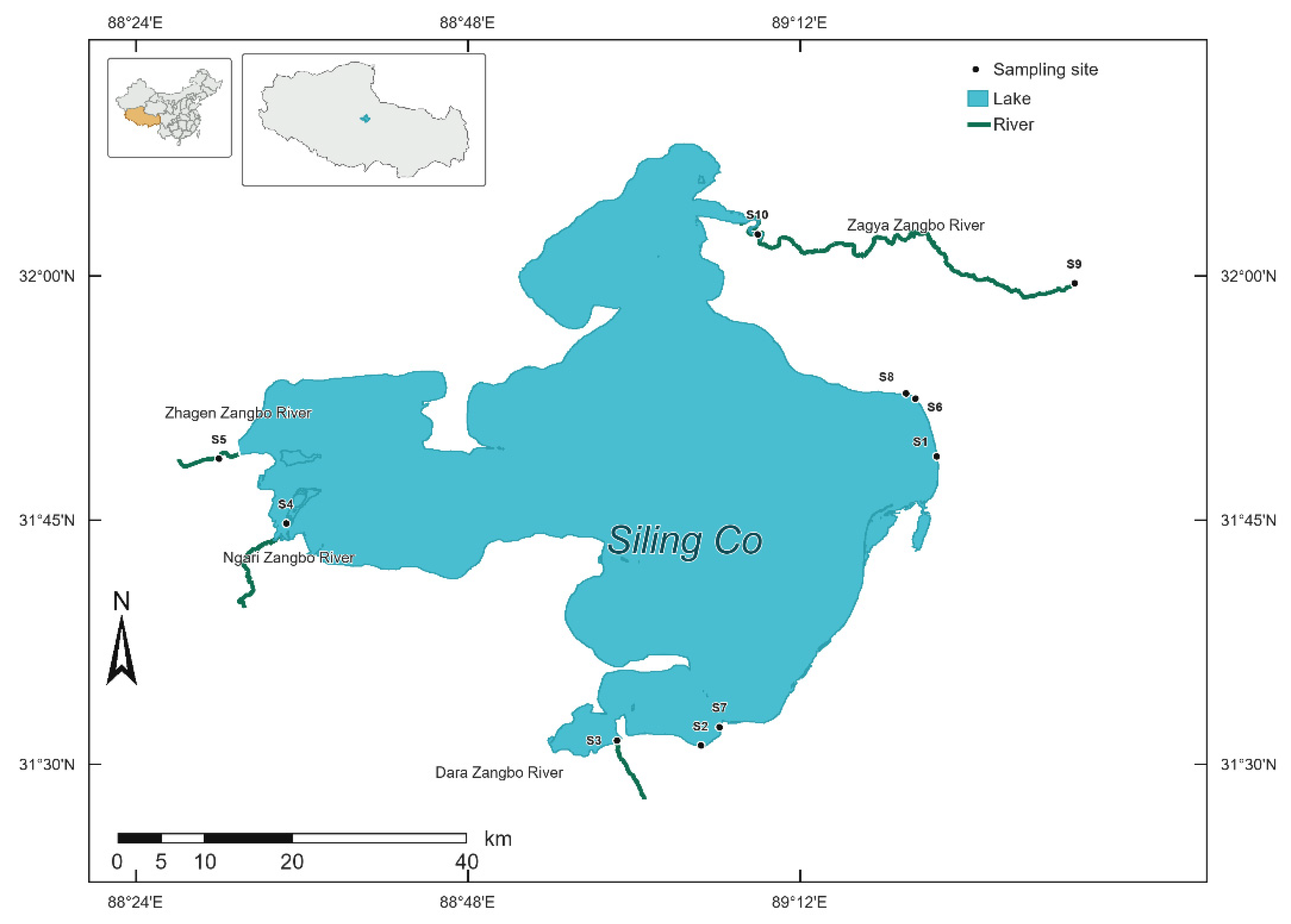
Figure 2.
PCA biplot of environmental variables in the Siling Co lake–river confluence zone. Points represent samples, colours indicate water-body type, and point shapes denote sampling periods. Arrows indicate the loading directions and relative contributions of environmental variables to PC1 and PC2. Lake samples were more tightly clustered than River samples, consistent with comparatively stable environmental conditions.
Figure 2.
PCA biplot of environmental variables in the Siling Co lake–river confluence zone. Points represent samples, colours indicate water-body type, and point shapes denote sampling periods. Arrows indicate the loading directions and relative contributions of environmental variables to PC1 and PC2. Lake samples were more tightly clustered than River samples, consistent with comparatively stable environmental conditions.
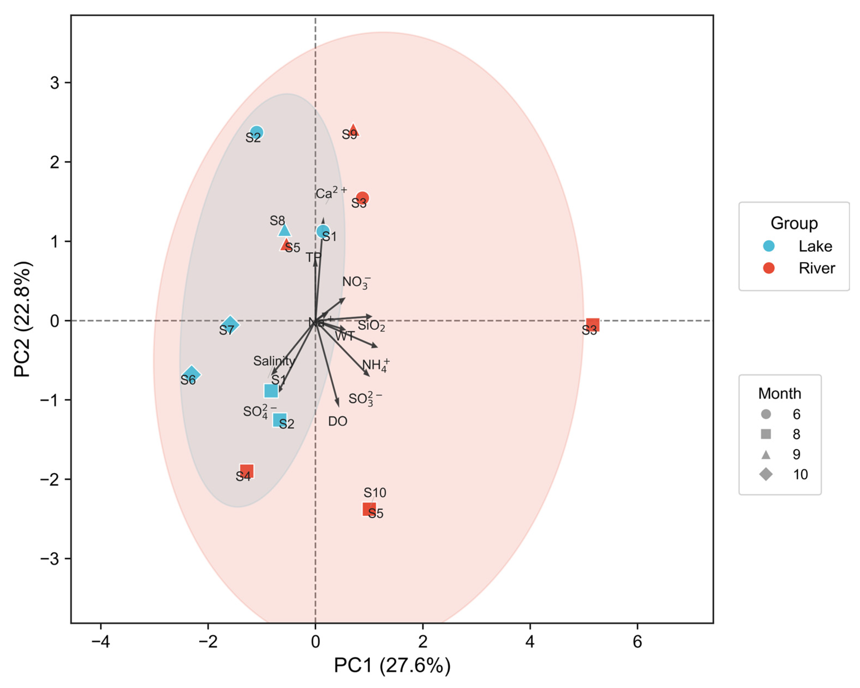
Figure 3.
Phylum-level relative composition of phytoplankton in the Siling Co lake–river confluence zone. (A) Relative cell density. (B) Relative biomass. Samples were grouped as Lake or River and ordered within each group by scores on the first axis of the environmental PCA.
Figure 3.
Phylum-level relative composition of phytoplankton in the Siling Co lake–river confluence zone. (A) Relative cell density. (B) Relative biomass. Samples were grouped as Lake or River and ordered within each group by scores on the first axis of the environmental PCA.
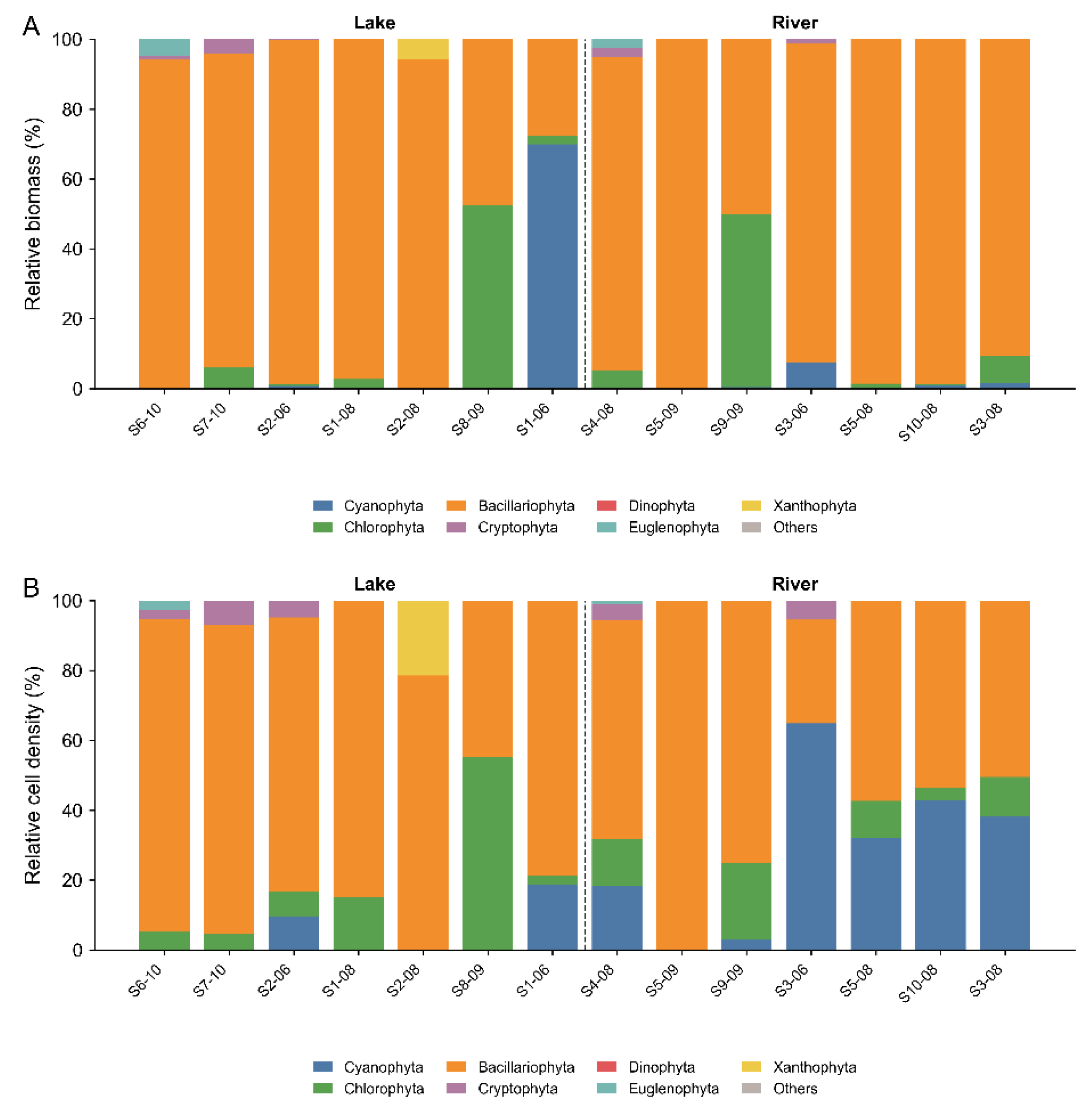
Figure 4.
Genus-level phytoplankton composition and distribution of dominant genera. (A) Relative cell-density composition of dominant genera in Lake and River samples. (B) Relative biomass composition of dominant genera in Lake and River samples.
Figure 4.
Genus-level phytoplankton composition and distribution of dominant genera. (A) Relative cell-density composition of dominant genera in Lake and River samples. (B) Relative biomass composition of dominant genera in Lake and River samples.
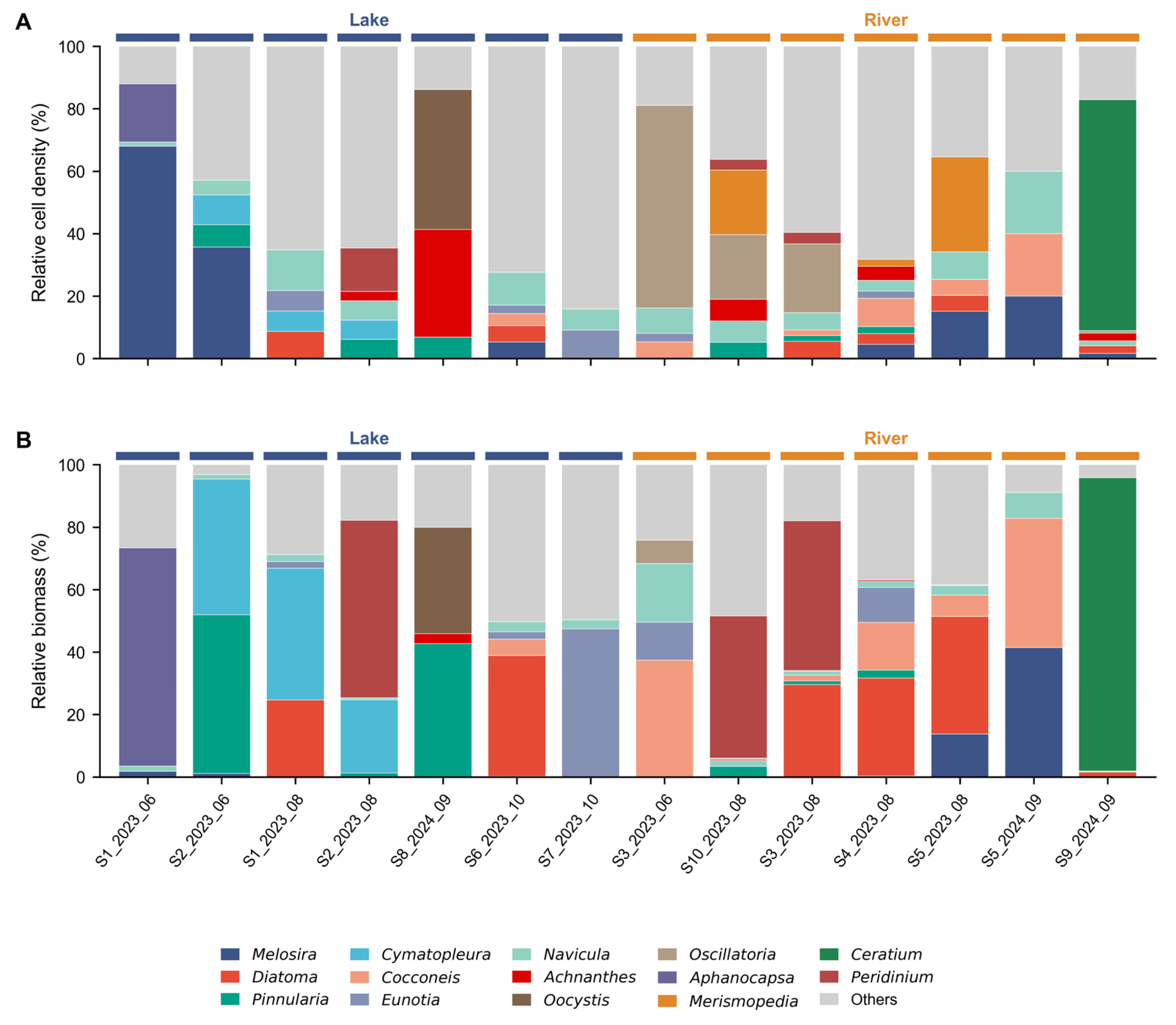
Figure 5.
Distribution of dominant phytoplankton genera at the genus level. (A) Standardized distribution of relative cell density of dominant genera across samples. (B) Standardized distribution of relative biomass of dominant genera across samples.
Figure 5.
Distribution of dominant phytoplankton genera at the genus level. (A) Standardized distribution of relative cell density of dominant genera across samples. (B) Standardized distribution of relative biomass of dominant genera across samples.
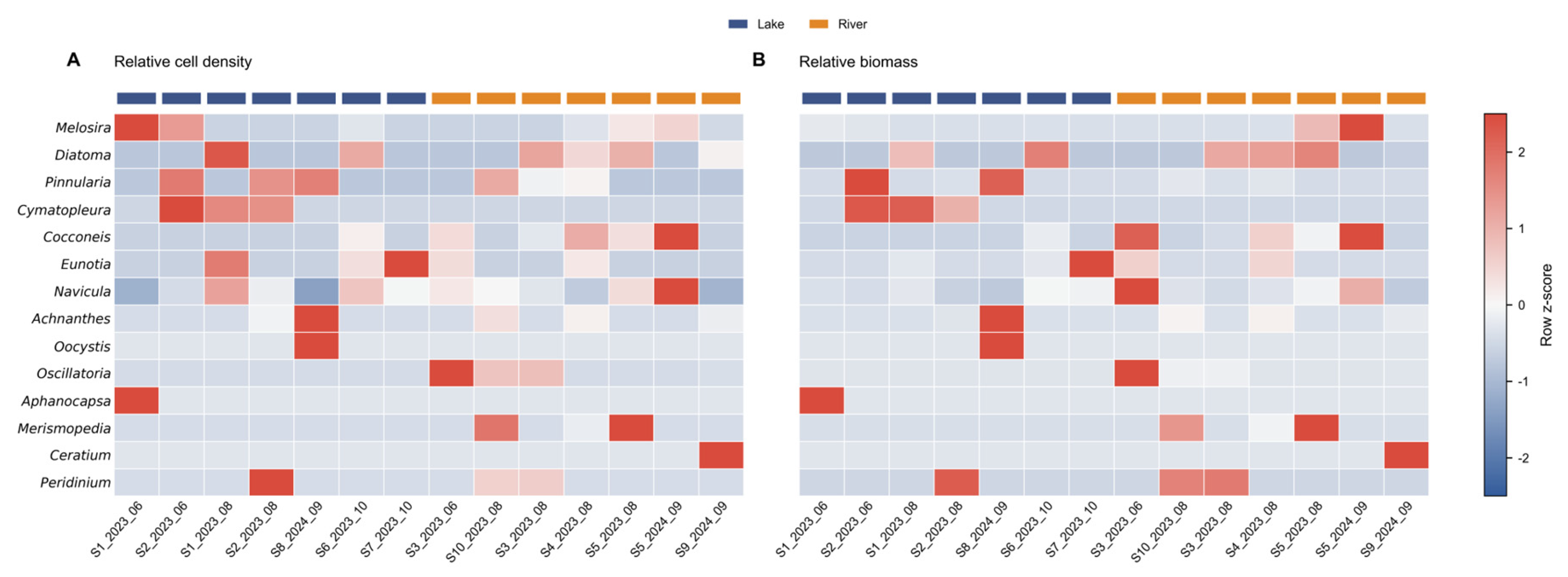
Figure 6.
Total phytoplankton cell density, total biomass, and α-diversity metrics across sampling periods. Circles and triangles represent Lake and River samples, respectively, and black lines indicate the median for each sampling period. Because month and year were not fully crossed in the sampling design, the results represent differences among sampling periods rather than strictly seasonal effects.
Figure 6.
Total phytoplankton cell density, total biomass, and α-diversity metrics across sampling periods. Circles and triangles represent Lake and River samples, respectively, and black lines indicate the median for each sampling period. Because month and year were not fully crossed in the sampling design, the results represent differences among sampling periods rather than strictly seasonal effects.
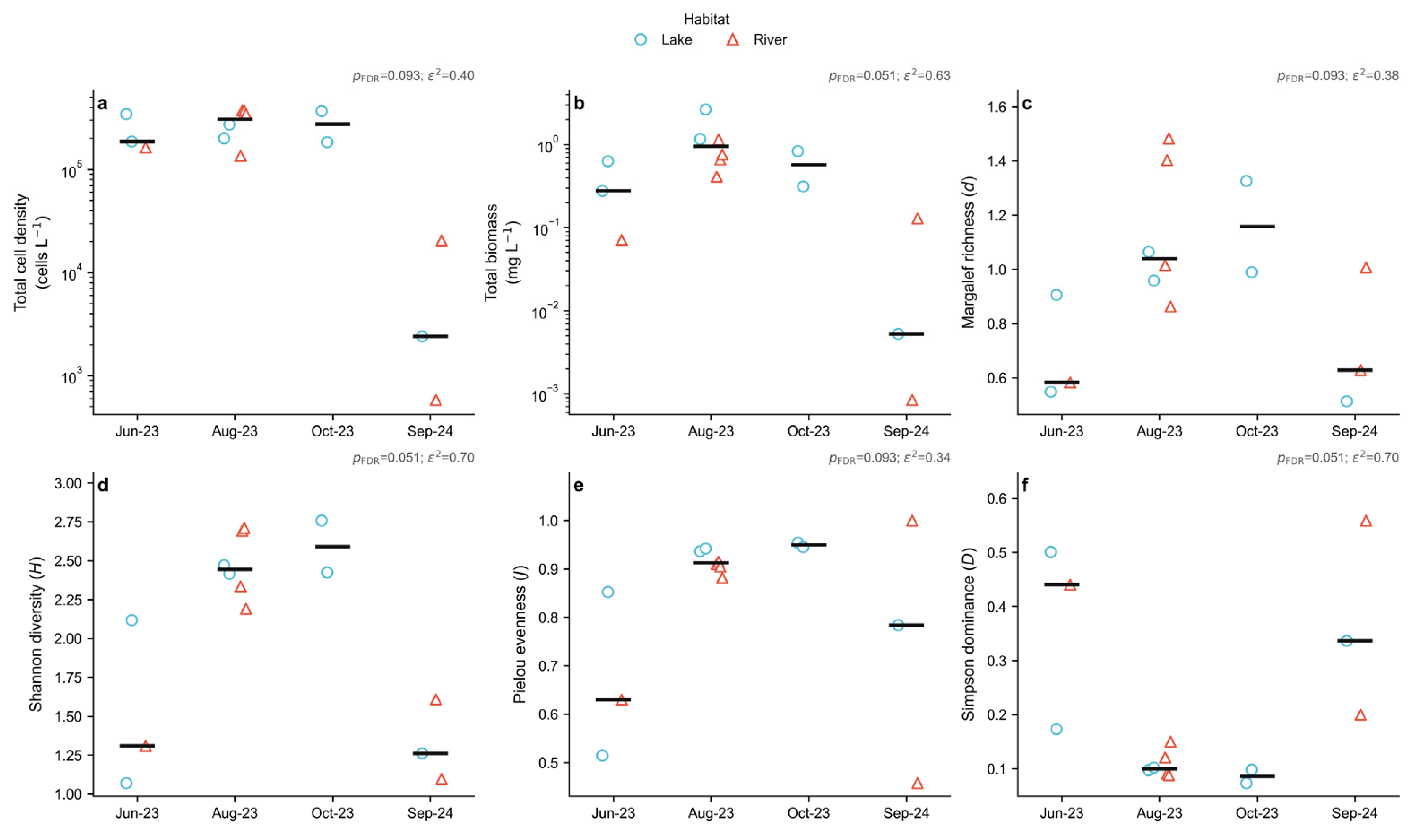
Figure 7.
PCoA of phytoplankton communities based on genus-level cell density (A) and biomass (B). Bray–Curtis dissimilarities were calculated from relative-abundance and Hellinger-transformed community data. Colours indicate water-body type, point shapes denote sampling periods, and shaded ellipses represent the 95% distribution range.
Figure 7.
PCoA of phytoplankton communities based on genus-level cell density (A) and biomass (B). Bray–Curtis dissimilarities were calculated from relative-abundance and Hellinger-transformed community data. Colours indicate water-body type, point shapes denote sampling periods, and shaded ellipses represent the 95% distribution range.
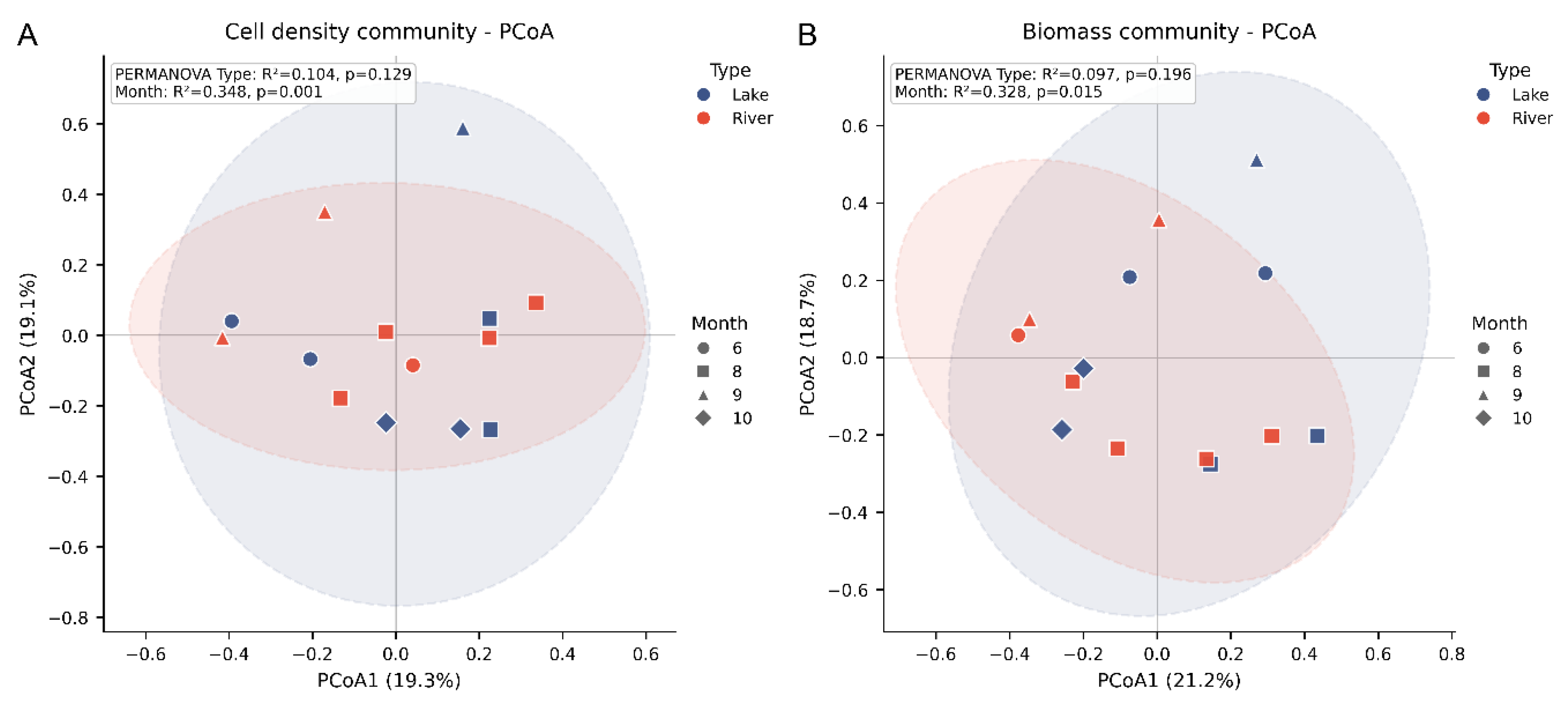
Figure 8.
Spearman correlations between overall phytoplankton metrics and environmental variables. * indicate significant associations after within-family FDR correction.
Figure 8.
Spearman correlations between overall phytoplankton metrics and environmental variables. * indicate significant associations after within-family FDR correction.
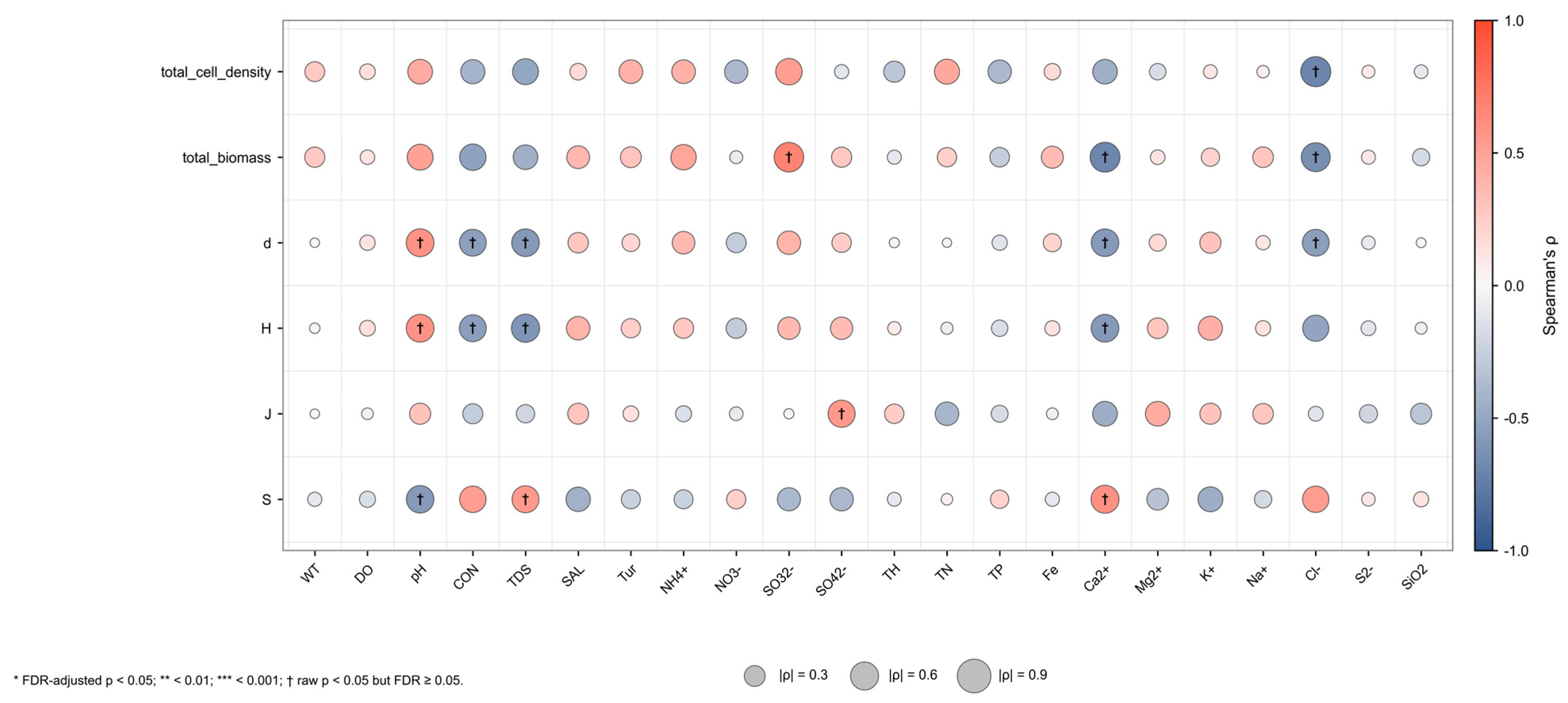
Figure 9.
Spearman correlations between phylum-level phytoplankton composition and environmental variables. (A) Cell density. (B) Biomass. * indicate significant associations after within-family FDR correction.
Figure 9.
Spearman correlations between phylum-level phytoplankton composition and environmental variables. (A) Cell density. (B) Biomass. * indicate significant associations after within-family FDR correction.
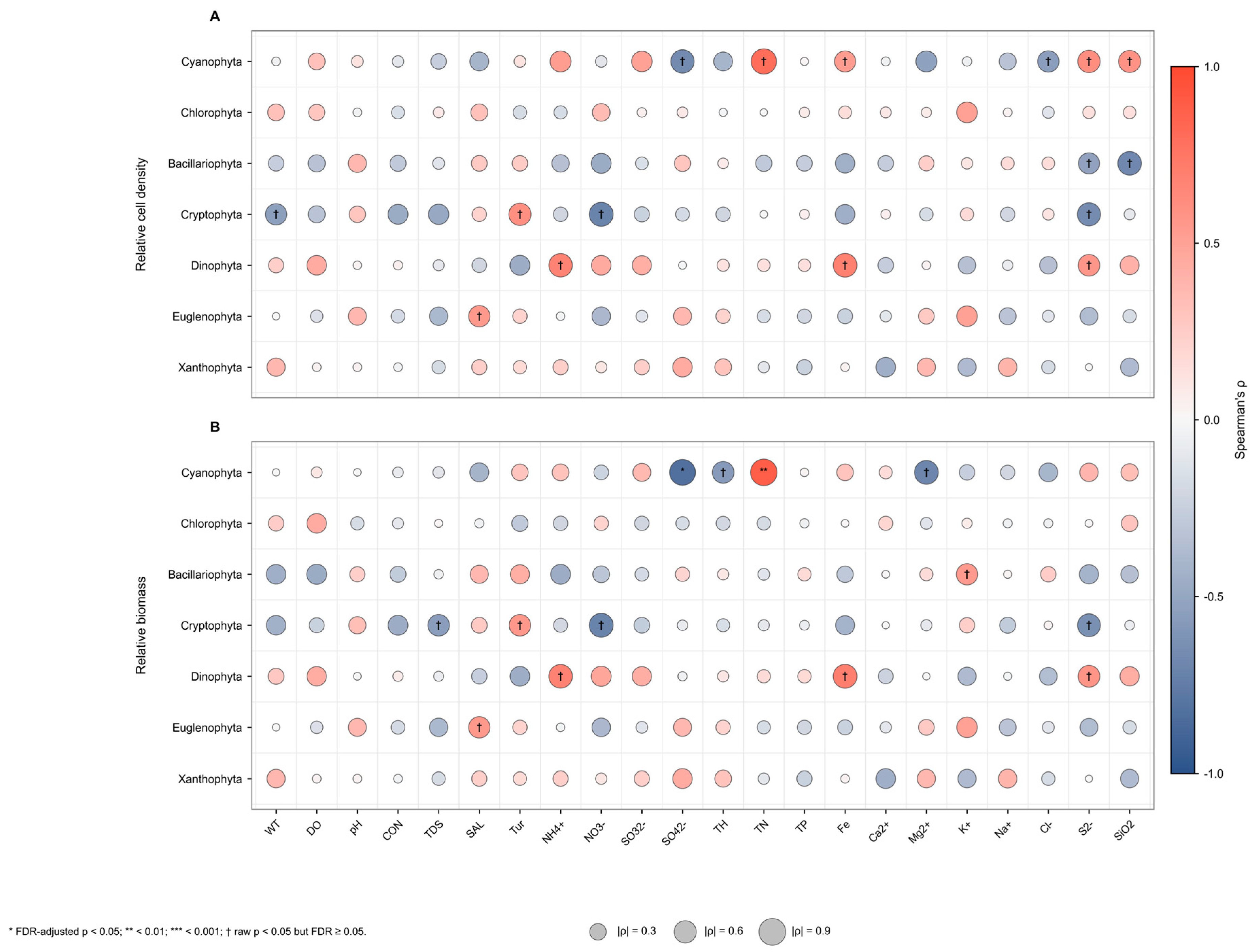
Figure 10.
Distance-based redundancy analysis of environmental variables and genus-level phytoplankton community composition. (A) Biomass db-RDA, with Cl− retained in the final model. (B) Cell-density db-RDA, with pH and SiO2 retained in the final model. Red arrows indicate retained environmental variables, whereas grey arrows indicate the correlation directions of major genera.
Figure 10.
Distance-based redundancy analysis of environmental variables and genus-level phytoplankton community composition. (A) Biomass db-RDA, with Cl− retained in the final model. (B) Cell-density db-RDA, with pH and SiO2 retained in the final model. Red arrows indicate retained environmental variables, whereas grey arrows indicate the correlation directions of major genera.
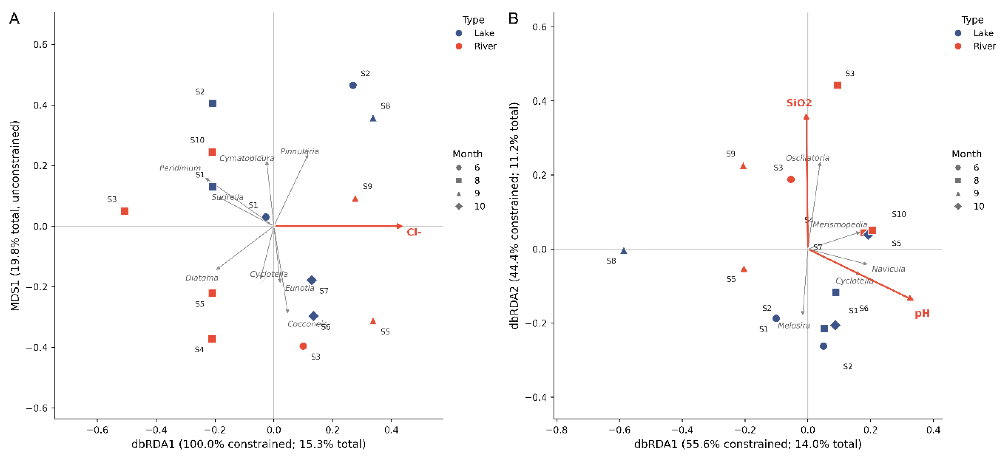
Figure 11.
Mantel relationships between environmental variable groups and phytoplankton community dissimilarity. Bubble size represents the absolute value of Mantel r, and colour indicates significance after FDR correction.
Figure 11.
Mantel relationships between environmental variable groups and phytoplankton community dissimilarity. Bubble size represents the absolute value of Mantel r, and colour indicates significance after FDR correction.
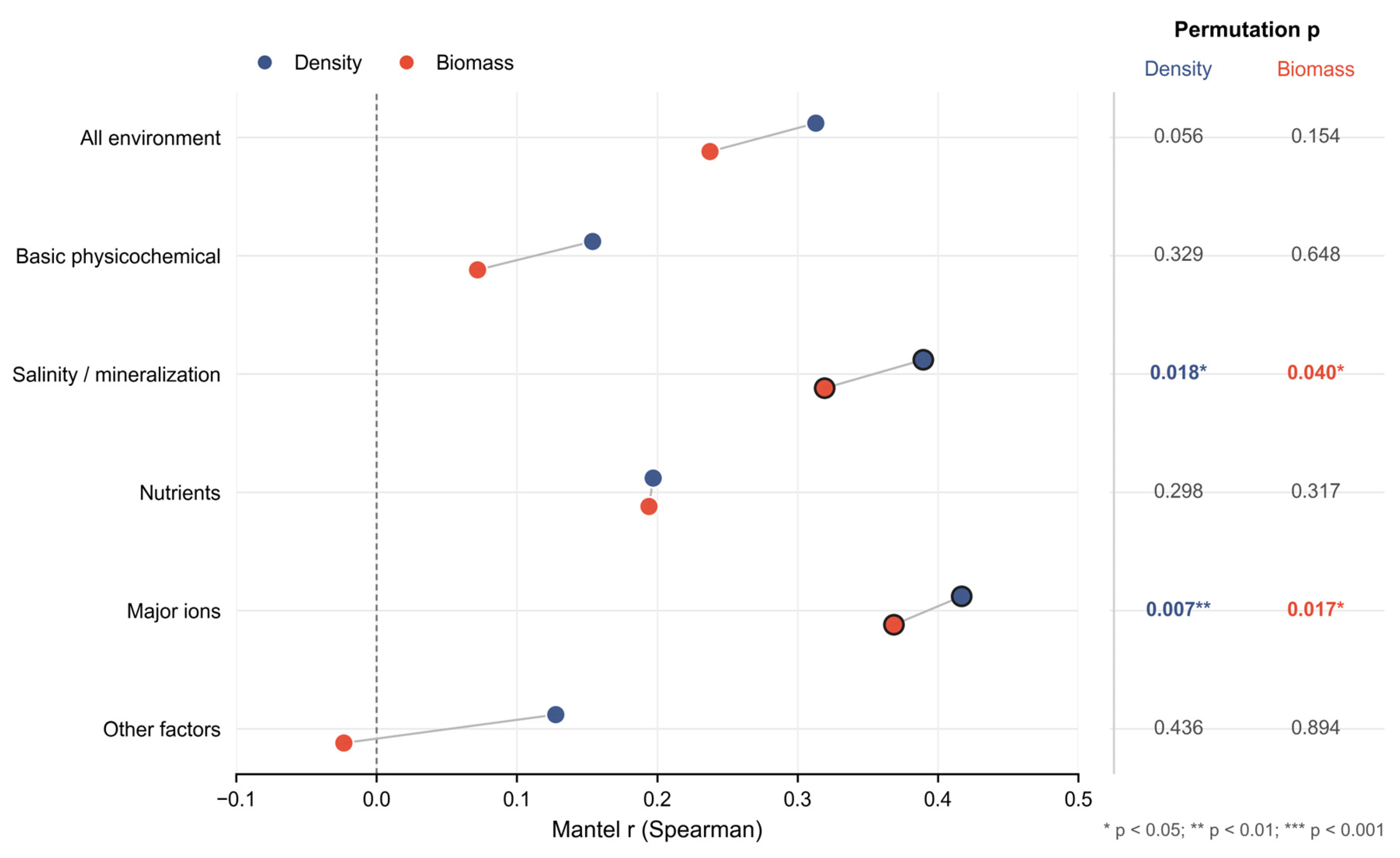
Figure 12.
Multi-method evidence for key environmental drivers of phytoplankton communities in the Siling Co lake–river confluence zone. (A) Evidence matrix. (B) Integrated ranking. Scores reflect consistency of evidence across methods rather than the causal effect size of environmental factors.
Figure 12.
Multi-method evidence for key environmental drivers of phytoplankton communities in the Siling Co lake–river confluence zone. (A) Evidence matrix. (B) Integrated ranking. Scores reflect consistency of evidence across methods rather than the causal effect size of environmental factors.
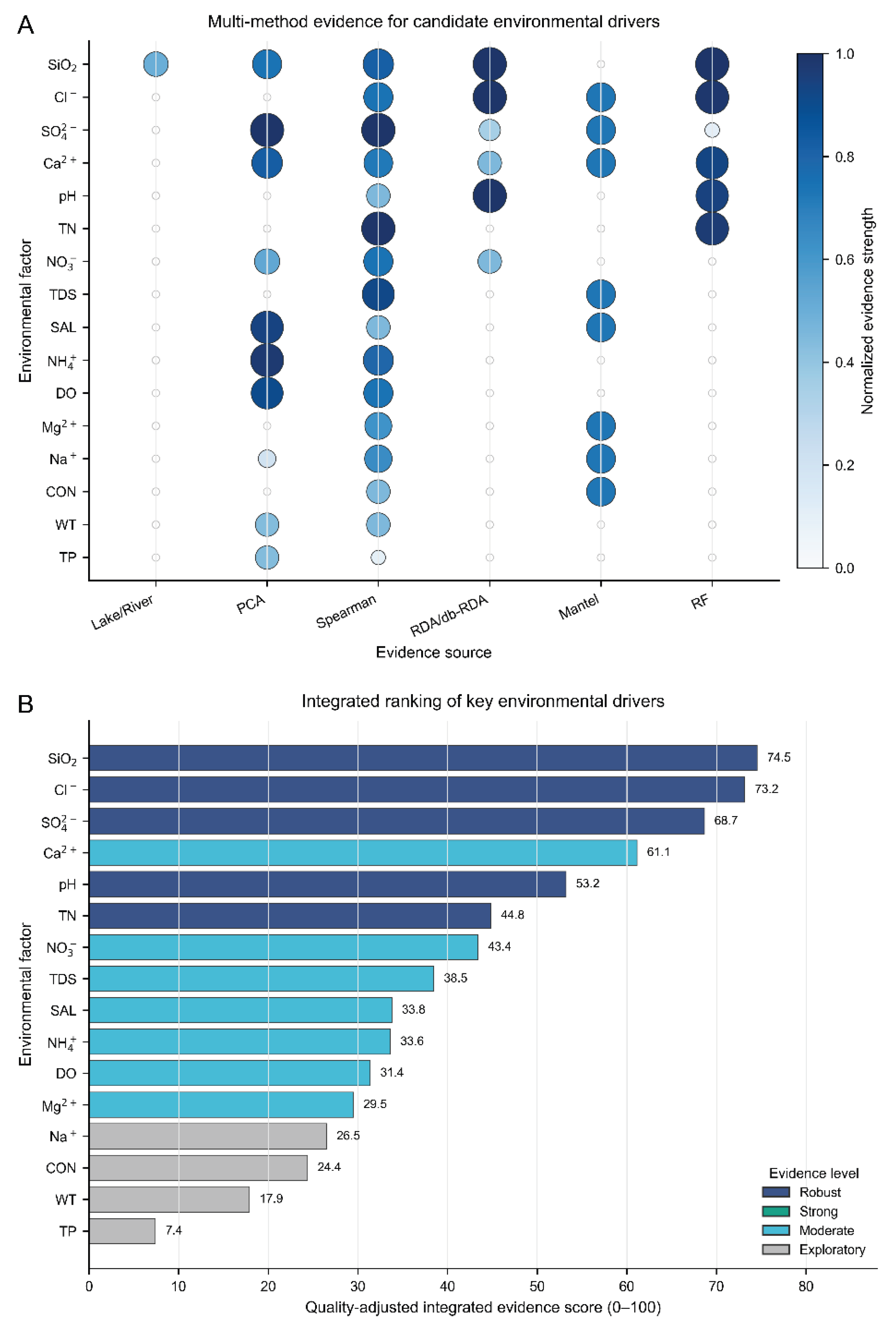
Table 2.
Strong Spearman correlations among environmental variables after FDR correction.
| Variable 1 | Variable 2 | ρ | Unadjusted P | FDR-adjusted P | Direction |
|---|---|---|---|---|---|
| Fe | S2− | 0.828 | 0.0002532 | 0.0205 | Positive |
| pH | TDS | −0.824 | 0.0002874 | 0.0205 | Negative |
| TDS | CON | 0.815 | 0.0003838 | 0.0205 | Positive |
| pH | CON | −0.811 | 0.0004314 | 0.0205 | Negative |
Strong correlations were defined as |ρ| ≥ 0.70 with an FDR-adjusted P < 0.05 (n = 14).
Table 5.
PERMANOVA results for differences in phytoplankton community structure.
| Community matrix | Model | R2 | pseudo-F | P | Result |
|---|---|---|---|---|---|
| Cell density | Type | 0.104 | 1.396 | 0.1292 | ns |
| Cell density | Month | 0.348 | 1.776 | 0.0014 | Significant |
| Cell density | Year | 0.142 | 1.991 | 0.0142 | Significant* |
| Cell density | Type + Month | 0.449 | 1.834 | 0.0006 | Significant |
| Cell density | Environmental PC1 + PC2 | 0.201 | 1.379 | 0.0754 | ns |
| Biomass | Type | 0.098 | 1.296 | 0.1956 | ns |
| Biomass | Month | 0.328 | 1.627 | 0.0148 | Significant |
| Biomass | Year | 0.130 | 1.789 | 0.0326 | Significant* |
| Biomass | Type + Month | 0.445 | 1.800 | 0.0024 | Significant |
| Biomass | Environmental PC1 + PC2 | 0.195 | 1.333 | 0.1190 | ns |
ns indicates non-significance. Asterisks indicate that Year was confounded with Month; therefore, these results are interpreted as differences among sampling periods rather than independent interannual effects. Significance was assessed using 4,999 permutations.
Table 6.
Final db-RDA models for genus-level phytoplankton community composition.
| Community matrix | Final environmental variables | R2 | Adjusted R2 | pseudo-F | Model P |
|---|---|---|---|---|---|
| Cell density | pH; SiO2 | 0.252 | 0.116 | 1.850 | 0.0007 |
| Biomass | Cl− | 0.153 | 0.083 | 2.174 | 0.0027 |
Conditional permutation P values for pH and SiO2 in the cell-density model were 0.0076 and 0.0294, respectively. The conditional permutation P value for Cl− in the biomass model was 0.0030.
Table 7.
Integrated ranking and evidence levels for key environmental drivers.
| Rank | Environmental factor | Integrated score | Number of supporting methods | Direct evidence | Evidence level |
|---|---|---|---|---|---|
| 1 | SiO2 | 74.5 | 5 | Yes | Robust |
| 2 | Cl− | 73.2 | 4 | Yes | Robust |
| 3 | SO42− | 68.7 | 4 | Yes | Robust |
| 4 | Ca2+ | 61.1 | 5 | No | Moderate |
| 5 | pH | 53.2 | 3 | Yes | Robust |
| 6 | TN | 44.8 | 2 | Yes | Robust |
Integrated scores were weighted across multiple evidence types and adjusted for the proportion of missing values. They represent consistency of evidence rather than causal effect sizes.
Disclaimer/Publisher’s Note: The statements, opinions and data contained in all publications are solely those of the individual author(s) and contributor(s) and not of MDPI and/or the editor(s). MDPI and/or the editor(s) disclaim responsibility for any injury to people or property resulting from any ideas, methods, instructions or products referred to in the content. |
© 2026 by the authors. Licensee MDPI, Basel, Switzerland. This article is an open access article distributed under the terms and conditions of the Creative Commons Attribution (CC BY) license (http://creativecommons.org/licenses/by/4.0/).
Copyright: This open access article is published under a Creative Commons CC BY 4.0 license, which permit the free download, distribution, and reuse, provided that the author and preprint are cited in any reuse.